The first law of differential entropy and holographic complexity

Abstract

We construct the CFT dual of the first law of spherical causal diamonds in three-dimensional AdS spacetime. A spherically symmetric causal diamond in AdS₃ is the domain of dependence of a spatial circular disk with vanishing extrinsic curvature. The bulk first law relates the variations of the area of the boundary of the disk, the spatial volume of the disk, the cosmological constant and the matter Hamiltonian. In this paper we specialize to first-order metric variations from pure AdS to the conical defect spacetime, and the bulk first law is derived following a coordinate based approach. The AdS/CFT dictionary connects the area of the boundary of the disk to the differential entropy in CFT₂, and assuming the ‘complexity=volume’ conjecture, the volume of the disk is considered to be dual to the complexity of a cutoff CFT. On the CFT side we explicitly compute the differential entropy and holographic complexity for the vacuum state and the excited state dual to conical AdS using the kinematic space formalism. As a result, the boundary dual of the bulk first law relates the first-order variations of differential entropy and complexity to the variation of the scaling dimension of the excited state, which corresponds to the matter Hamiltonian variation in the bulk. We also include the variation of the central charge with associated chemical potential in the boundary first law. Finally, we comment on the boundary dual of the first law for the Wheeler-deWitt patch of AdS, and we propose an extension of our CFT first law to higher dimensions.

1 Introduction

Deriving gravitational thermodynamics of black holes Bekenstein:1973ur ; Bardeen:1973gs ; Hawking:1974sw from a microscopic perspective remains one of the guiding principles in the quest for quantum gravity. The microscopic state counting of black hole entropy Strominger:1996sh is considered to be one of the major successes of string theory. Later, this microscopic derivation of black hole entropy was reinterpreted Strominger:1997eq in terms of the Anti-de Sitter (AdS)/ Conformal Field Theory (CFT) correspondence Maldacena:1997re , where the entropy of three-dimensional AdS black holes Banados:1992wn ; Banados:1992gq matches with the thermodynamic entropy in two-dimensional CFTs Cardy:1986ie . In higher dimensions, it has also been argued that the mass, entropy and temperature of AdS black holes can be identified with the energy, entropy and temperature of a thermal state in the dual CFT at high temperature Witten:1998zw .

Furthermore, the correspondence between gravitational entropy and CFT entropy can be extended to the entanglement entropy of subregions on the conformal boundary of AdS. The Ryu-Takayagani (RT) formula Ryu:2006bv ; Ryu:2006ef states that the entanglement entropy of a subregion $\mathcal{R}$ in the CFT is, to leading order in Newton’s constant, dual to the Bekenstein-Hawking entropy $A/(4G)$ of the minimal bulk surface which intersects the conformal boundary at $\partial\mathcal{R}$. The entanglement entropy satisfies a first law-like relation, which is the quantum generalization of the first law of thermodynamics Blanco:2013joa ; Wong:2013gua . An important result in AdS/CFT shows that the linearized gravitational dynamics in the bulk emerge from the RT formula and the first law of entanglement on the boundary Faulkner:2013ica .

More recently, the area of non-extremal codimension-two surfaces in three-dimensional AdS spacetime, which are not necessarily homologous to the boundary, was related to the notion of differential entropy in $2d$ CFTs, via equation (8) Balasubramanian:2013rqa ; Balasubramanian:2013lsa . The authors discovered that closed curves in a spatial slice of AdS₃ can be reconstructed by adding and subtracting boundary-anchored geodesics tangent to the curve. Since RT surfaces in AdS₃ are boundary-anchored geodesics, they were able to express the length (‘area’) of the closed curve in terms of an integral over entanglement entropies, associated to the boundary intervals subtended by the geodesics, which they dubbed ‘differential entropy’. This new field theoretic quantity can be qualitatively interpreted as the uncertainty about the global state for local observers who make measurements for a finite time in the CFT, because the exterior of a bulk closed curve is naturally associated to a time strip in the dual CFT. The formalism of differential entropy was extended to higher dimensions Myers:2014jia ; Czech:2014wka ; Balasubramanian:2018uus , covariant set-ups Hubeny:2014qwa ; Headrick:2014eia , bulk curves near horizons or singularities Balasubramanian:2014sra , bulk points and distances Czech:2014ppa , the Poincaré and Rindler wedges of AdS Espindola:2017jil ; Espindola:2018ozt , and it was reinterpreted in terms of kinematic space in Czech:2015qta , reviewed in section 2.1. In the present work, in similarity to the first law of entanglement, we derive a first law of differential entropy for a holographic CFT₂.

To construct the first law of differential entropy we find inspiration from the bulk side, where gravitational thermodynamics has been extended to spherical causal diamonds in maximally symmetric spacetimes (hence including in AdS) Jacobson:2015hqa ; Jacobson:2018ahi . Spherically symmetric causal diamonds are defined as the future and past domain of dependence of spherical, codimension-two, spatial regions with vanishing extrinsic curvature (see figure 4). These spherical regions in AdS are relevant for our purposes, since their boundary area is dual to differential entropy in the CFT. In general, maximally symmetric causal diamonds admit only a conformal Killing vector $\zeta$, instead of a true Killing vector like for stationary black holes, although in certain limits $\zeta$ becomes a true Killing vector (e.g. for Rindler spacetime and the static patch of de Sitter spacetime). Hence, generic maximally symmetric diamonds are only ‘conformally stationary’, but this seems to be sufficient for them to behave as thermodynamic equilibrium states under gravitational perturbations. The variational relation to nearby solutions of these diamonds in Einstein gravity is given by Jacobson:2015hqa ; Jacobson:2018ahi

$$\delta H^{\text{mat}}_{\zeta}=\frac{1}{8\pi G}\left(-\kappa\delta A+\kappa k\delta V-V_{\zeta}\delta\Lambda\right).$$ (1)

This is the so-called first law of causal diamonds. Let us briefly explain the notation: $H_{\zeta}^{\text{mat}}$ is the matter Hamiltonian generating the evolution of classical matter fields along the conformal Killing flow, $A$ is the area of the edge of the diamond, $V$ is the volume of the maximal slice, $k$ is the trace of the extrinsic curvature of the edge as embedded in the maximal slice, $\kappa$ is the surface gravity associated to $\zeta$, and $V_{\zeta}$ is the ‘thermodynamic volume’ of the maximal slice conjugate to the variation of the cosmological constant $\Lambda$.

In this paper we restrict to causal diamonds associated to circular disks in AdS₃. The main goal is to derive a dual first law in a CFT₂ with a large central charge. For simplicity, we consider excited states in the CFT dual to a conical defect in AdS, which arises due to the presence of a classical point particle Deser:1983tn ; Deser:1983nh . For this setting we prove the first law of causal diamonds by fixing the global coordinates of AdS₃ and changing the metric and classical matter fields from pure AdS₃ to conical AdS₃ (see section 3.2). We compute the variation of the bulk area, volume and matter Hamiltonian due to changes in the boundary interval size (associated to geodesics tangent to the boundary of the disk), the conical defect parameter and the cosmological constant. By combining these variations in a particular way we find that the term proportional to the variation of the boundary interval size drops out of the first law and we reproduce (1). The main difference compared to Jacobson:2018ahi is that we derive the first law using a fixed coordinate approach, rather than Wald’s covariant phase space formalism Wald:1993nt ; Iyer:1994ys . The latter approach is more general since it holds for arbitrary variations to nearby solutions, whereas here we consider only metric perturbations to conical AdS. The advantage of our approach is, however, that it provides a controlled setting to compare variations in AdS and in the CFT.

The boundary dual to the first law of causal diamonds can be derived in a similar fashion. Two important ingredients in our boundary first law are differential entropy $S_{\text{diff}}$ and a version of holographic complexity $\mathcal{C}$ based on the ‘complexity=volume’ proposal and the volume formula for finite bulk regions in Abt:2017pmf ; Abt:2018ywl . Both notions can be formulated in the kinematic space formalism, and are defined in terms of entanglement entropies, cf. (8) and (31). The holographic dictionary used in this paper reads (with $L$ the AdS radius)

$$S_{\text{diff}}=\frac{A}{4G}\qquad\text{and}\qquad\mathcal{C}=\frac{V}{4GL}.$$ (2)

We compute the variations of $S_{\text{diff}}$ and $\mathcal{C}$ with respect to the subregion size $\alpha$, the scaling dimension $\Delta$ and the central charge $c$. The scaling dimension is associated to the (twist) operator acting on the vacuum state, and the central charge is varied in the space of CFTs. We assume $\Delta\sim c\gg 1$ such that the CFT excited state is dual to a classical geometry in the bulk. Varying $c$ corresponds to changing the coupling constants $G$ and $\Lambda$ in the bulk. The combination of the variations of $S_{\text{diff}}$ and $\mathcal{C}$ yields the following CFT first law

$$\delta E=T\delta S_{\text{diff}}+\nu\delta\mathcal{C}+\mu\delta c.$$ (3)

We call this the first law of differential entropy. Here $E$ is a rescaled energy in the CFT, whose variation is given by

$$\delta E=\kappa f(\alpha)\delta\Delta\qquad\text{with}\qquad f(\alpha)=\frac{1}{\cos\alpha}-\frac{\sin\alpha}{\cos\alpha},$$ (4)

where $\kappa$ is an arbitrary normalization which could depend on $\alpha$ and corresponds in the bulk to the surface gravity of the diamond. The function $f(\alpha)$ is positive in the range $\alpha\in[0,\pi/2]$ and is related to the norm of the bulk conformal Killing vector $\zeta$ evaluated at the center of the diamond, via $\sqrt{-\zeta\cdot\zeta}\big{|}_{O}=\kappa Lf(\alpha)$. Further, the boundary energy $E$ is dual to the bulk matter Hamiltonian $H_{\zeta}^{\text{mat}}$ (see section 3.2.3). The conjugate quantities in the boundary first law depend on the normalization and subregion size as follows

$$T=-\frac{\kappa}{2\pi},\qquad\nu=\frac{\kappa}{2\pi}\frac{1}{\cos\alpha},\qquad\text{and}\qquad\mu=\frac{1}{c}\big{(}\!-TS_{\text{diff}}^{\text{vac}}-\nu\mathcal{C}_{\text{vac}}\big{)}=\frac{\kappa}{2\pi}\frac{\pi}{3}f(\alpha)\,.$$ (5)

In the paper we set $\kappa=2\pi.$ Here, $\mu$ is a chemical potential to changing the number of field degrees of freedom in the CFT, and $\nu$ is the energy cost of changing the complexity. The formal ‘temperature’ $T$ is negative, in line with the gravitational thermodynamics of causal diamonds Jacobson:2018ahi . In section 2.3 we study two limiting cases of the boundary first law: large and small boundary subregions. The zero subregion size limit ($\alpha\to 0$), cf. (85), is dual to the first law for the ‘Wheeler-deWitt’ (WdW) patch of pure AdS, which is a limiting case of the first law of causal diamonds Jacobson:2018ahi . In related work, a similar WdW first law was derived for coherent states in the bulk and on the boundary, without the area variation, and argued to be dual to the ‘first law of complexity’ Bernamonti:2019zyy ; Bernamonti:2020bcf or to the boundary symplectic form Belin:2018fxe ; Belin:2018bpg . Hence, our first law (3) can be viewed as an extension of the first law of complexity which includes the variation of differential entropy and central charge, and which depends on the boundary subregion size $\alpha$ (corresponding to finite bulk regions).

The plan of the paper is as follows. In section 2 we derive the first law of differential entropy and holographic complexity. Section 3 is devoted to the first law of causal diamonds applied to the present geometric setting. We match the boundary first law and bulk first law in section 4. We first show how the former follows from the latter, and afterwards we discuss a possible higher dimensional generalization of the boundary first law. We end with concluding remarks and an outlook in section 5.

Finally, we have a total of four appendices. Appendix A discusses the embedding formalism and several coordinate systems for pure AdS₃ and conical AdS₃. In appendix B we compute the geodesic equation and the chord length of finite geodesic arcs in conical AdS. Further, in appendix C we derive the boundary conformal Killing vector of a causal diamond on the cylinder, both from the generators of the conformal group on the cylinder and from the boundary limit of the boost Killing vector of AdS-Rindler space. Appendix D studies the contributions from the variation of $G$ and $\Lambda$ in the first law of causal diamonds, using the covariant phase space formalism, and shows that the term proportional to the variation of Newton’s constant vanishes in the first law.

2 A first law in CFT₂

We are interested in studying the physics of bounded regions in the bulk from a field theory perspective, in the context of the AdS/CFT correspondence. For simplicity, we restrict to AdS₃/CFT₂ and we focus on the example of a circular disk $D$ of coordinate radius $R$ inside a time slice of AdS. A gravitational first law (1) has recently been derived for metric perturbations of such disks in pure AdS which satisfy the linearized Einstein equation Jacobson:2018ahi . For a gravitational theory with a boundary dual field theory, it is a natural question whether a CFT version of such a gravitational first law exists. The CFT first law is an unexplored subject within the AdS/CFT literature, and in what follows we will derive a non-trivial variational relation between various boundary quantities that is dual to the bulk first law. This establishes a new relational entry in the AdS/CFT dictionary.

There are two terms in the gravitational first law which allow for an immediate holographic interpretation in AdS₃/CFT₂: the area variation of the boundary of the disk and the volume variation of the disk. First, there is a fair amount of literature that investigates the CFT dual of the area of an arbitrary differentiable curve on a spatial slice of AdS₃ Balasubramanian:2013rqa ; Balasubramanian:2013lsa ; Czech:2014ppa ; Myers:2014jia ; Headrick:2014eia ; Espindola:2017jil . This goes by the name of differential entropy, which is a derived quantity from entanglement entropy and is related to the area of any closed, differentiable bulk curve in a broad class of gravitational backgrounds. Second, we interpret the volume of the disk as holographic complexity, following the ‘complexity=volume’ conjecture Susskind:2014rva ; Stanford:2014jda . Although the disk is a finite bulk region, instead of an entire bulk time slice, we can still relate it to complexity because such a region corresponds to a CFT at a UV cutoff according to the well-known UV/IR correspondence Susskind:1998dq ; Peet:1998wn . We use the volume formula of Abt:2017pmf ; Abt:2018ywl to express the volume as a pure CFT quantity, an integral involving entanglement entropies analogous to differential entropy. An important technicality is that the volume formula only applies to quotients of pure AdS, which is sufficient for our purposes, since we take the perturbed geometry in the bulk first law to be AdS₃ with a conical singularity. Both differential entropy and the volume formula can be formulated in terms of the formalism of integral geometry and kinematic space Czech:2015qta , which we review shortly below.

Our setup is as follows. We work with Einstein gravity in locally AdS₃ spacetimes in global coordinates, and we mostly specialize to pure AdS and AdS with a conical singularity. The metric of the latter spacetime is

$$ds^{2}=-\left(\gamma^{2}+\frac{r^{2}}{L^{2}}\right)dt^{2}+\left(\gamma^{2}+\frac{r^{2}}{L^{2}}\right)^{-1}dr^{2}+r^{2}d\phi^{2},$$ (6)

where $\phi\in[0,2\pi)$ and $\gamma\in(0,1)$ parametrizes the departure away from pure AdS ($\gamma=1$). The dual CFT₂ lives on the conformal boundary, which is a Lorentzian cylinder. We fix the conformal frame on the boundary such that the CFT time is the same as global AdS time $t$, i.e. $ds^{2}_{\text{bndy}}=\lim_{r\to\infty}\frac{L^{2}}{r^{2}}ds^{2}$, and we distinguish the boundary angular coordinate $\theta$ from the bulk angular coordinate $\phi$ by shifting the origin. Thus, the boundary metric is

$$ds^{2}_{\text{bndy}}=-dt^{2}+L^{2}d\theta^{2}.$$ (7)

Note that the radius $L$ of the cylinder is equal to the AdS curvature radius in this frame.

2.1 Review of kinematic space

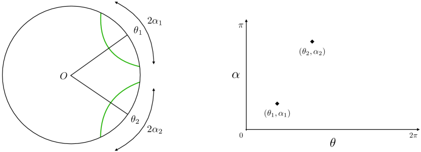
Figure 1: Left diagram: a time slice of pure AdS₃ containing two boundary anchored geodesics (in green) parametrized by $(\theta_{1},\alpha_{1})$ and $(\theta_{2},\alpha_{2})$. Right diagram: The associated two points in kinematic space with coordinate system $(\theta,\alpha)$, where $\theta$ denotes the midpoint of the boundary subregion in angular coordinates and $\alpha$ is the angular radius. The orientation of each geodesic is reversed by the transformation $(\theta,\alpha)\to(\pi+\theta,\pi-{\alpha})$, which exchanges the boundary subregion with its complement.

Kinematic space is the space of oriented spacelike geodesics in the bulk which are anchored on the boundary. In this article we restrict to static, locally AdS₃ geometries and to geodesics inside a time slice of those geometries. For vacuum AdS₃ kinematic space is the space of RT surfaces Ryu:2006bv ; Ryu:2006ef passing through a time slice. An equivalent parametrization of kinematic space is via the boundary subregion that the geodesics subtend: for a given pair $(\theta,\alpha)$ on the boundary, with $\theta$ the midpoint and $\alpha$ the opening angle of the subregion, there exists a unique oriented geodesic in the bulk (see figure 1). For the conical defect and BTZ geometry this is no longer the case: several geodesics (i.e. minimal and non-minimal geodesics) can be associated to a given boundary interval Balasubramanian:2014sra . Kinematic space for the conical defect spacetime can still be defined though as the space of oriented geodesics, thereby also taking into account non-minimal geodesics, but it cannot be defined as the space of boundary intervals (see Cresswell:2017mbk though for a CFT definition in terms of OPE blocks).

2.1.1 Differential entropy

The main idea behind differential entropy is to trace out every point of a closed bulk curve by unique boundary anchored geodesics of opening angle $\alpha(\theta)$ which are tangent to the bulk curve at that point. For a central bulk circle these geodesics are just the RT surfaces corresponding to subregions of a fixed, constant angular size $2\alpha$ for every angle $\theta$.

Differential entropy is defined as the $\theta$ integral over the derivative of the entanglement entropy $S(\alpha)$ with respect to $\alpha$ Balasubramanian:2013rqa ; Balasubramanian:2013lsa ; Czech:2014ppa

$$S_{\text{diff}}=\frac{1}{2}\int_{0}^{2\pi}d\theta\,\frac{dS(\alpha)}{d\alpha}\Bigg{|}_{\alpha=\alpha(\theta)}\qquad\text{(boundary)}.$$ (8)

Using the Ryu-Takayanagi formula $S=\ell/(4G)$, where $\ell$ is the length of the geodesic which is anchored at the boundary coordinates $\theta-\alpha$ and $\theta+\alpha$, the differential entropy can be expressed in terms of bulk quantities. It turns out that differential entropy is dual to the Bekenstein-Hawking entropy Bekenstein:1973ur ; Hawking:1974sw of the closed curve corresponding to the function $\alpha(\theta)$

$$S_{\text{diff}}=\frac{1}{8G}\int_{0}^{2\pi}d\theta\frac{d\ell(\alpha)}{d\alpha}\Bigg{|}_{\alpha=\alpha(\theta)}\!=\,\,\frac{A}{4G}\qquad\text{(bulk)}.$$ (9)

Here $A$ is the area (i.e. circumference) of the bulk curve and $G$ is the three-dimensional Newton constant. For example, for a CFT in the vacuum state on the cylinder, the entanglement entropy of a subregion of size $2\alpha$ with its complement is Calabrese:2004eu ; Holzhey:1994we

$$S^{\text{vac}}(\alpha)=\frac{c}{3}\log\left(\frac{2L}{\mu}\sin\alpha\right),$$ (10)

where $c$ is the central charge of the boundary CFT and $\mu$ is the UV cutoff scale. If we restrict the closed curve in the bulk to be a central circle, centered at the origin in global coordinates, then $\alpha$ is independent of $\theta$ for every point on the bulk curve, and the differential entropy is simply

$$S_{\text{diff}}^{\text{vac}}(\alpha)=\frac{\pi c}{3}\cot\alpha.$$ (11)

Note that the two scales $L$ and $\mu$ drop out in the differential entropy. Using the dictionary between the bulk radius and the boundary opening angle in pure AdS, given by $R=L\cot\alpha$ with $L$ the curvature radius of AdS, and the dictionary for the central charge $c=3L/(2G)$ Brown:1986nw , we find that the differential entropy is indeed equal to the circumference of the circle divided by $4G$

$$S_{\text{diff}}^{\text{vac}}(R)=\frac{2\pi R}{4G}.$$ (12)

This is only a simple example of the equality between differential entropy and the Bekenstein-Hawking entropy – which is nonetheless relevant for this paper – but the equality has been proven more generally for any closed, piecewise differentiable curve on a spatial slice of AdS₃ in Balasubramanian:2013lsa , and for time varying curves on arbitrary holographic backgrounds which possess a generalized planar symmetry in Headrick:2014eia . In what follows, the holographic dictionary between differential entropy and bulk area plays an important role in our boundary interpretation of the bulk first law.

There are several proposals in the literature for the physical interpretation of differential entropy. In the original paper Balasubramanian:2013rqa it has been conjectured that it signifies the amount of entanglement between quantum gravitational degrees of freedom associated to the interior and exterior of the bulk subregion. This was immediately challenged in the follow-up paper Balasubramanian:2013lsa , where it was suggested that the Hilbert space of quantum gravity does not factorize between the inside and outside of the bulk curve. This is because the exterior of the bulk curve is holographically dual to a finite time strip on the boundary cylinder and the density matrix on such a region still acts on the full Hilbert space of the CFT and not on a tensor factor. Instead, a separate interpretation was proposed based on the idea that observers who make measurements for a finite duration in time only have access to local CFT data, and not to the global state. As a result, the authors of Balasubramanian:2013lsa suggested that differential entropy measures the uncertainty in reconstructing the global quantum state from the local data collected by all observers in the finite time strip. However, this interpretation was contested in Swingle:2014nla since the global ground state cannot always be reconstructed with arbitrary high accuracy from local data. This is the case if, for example, there is a degeneracy of locally indistinguishable ground states. Therefore, the maximal global (‘reconstruction’) entropy of the global ground state does not always admit a precise bulk geometric interpretation.

Another interesting perspective was provided by Czech:2017zfq , which interprets differential entropy as the Wilson loop of the boundary modular Berry connection in kinematic space. This Berry connection relates the eigenspaces of modular Hamiltonians of different subsystems in the CFT. In the bulk the modular Berry connection ties two infinitesimally separated geodesics under the action of the bulk modular Hamiltonian, or more precisely the modular translation operator, which translates geodesics along a spatial direction of a fixed time slice. As mentioned above, the bulk disk is indeed mapped by a collection of such geodesics, so it is quite natural that the integrand in differential entropy serves as a connection in kinematic space. Finally, from a slightly different viewpoint, differential entropy also finds a quantum information theoretic definition in Czech:2014tva . In this language, the length and shape of the bulk curve is expressed in terms of a communication protocol called ‘constrained state merging’. The differential entropy is then the ‘entanglement cost’ of sending the state of the boundary subregion from one party to another, modulo locality constraints on the operations.

2.1.2 Volume formula

Next, we move to the term in the bulk first law proportional to the change in volume of the bulk subregion, which we interpret in terms of the change in holographic complexity. The volume of a maximal slice anchored at a boundary time slice in the eternal black hole spacetime has been conjectured to be dual to the complexity of the state on the boundary time slice in the CFT Susskind:2014moa ; Brown:2015bva . This ‘complexity=volume’ conjecture has been extended to the volume of the extremal bulk region bounded by a boundary subregion and the RT surface for this subregion, which is supposed to be dual to the complexity of the mixed state associated to the boundary subregion Alishahiha:2015rta ; Carmi:2016wjl . These conjectures have not been proven yet, due to a lack of understanding of complexity in interacting quantum field theories at strong coupling.

However, some progress in this subject has been made for the CFT dual of the volume of bulk subregions in (quotients of) pure AdS₃ Abt:2017pmf ; Abt:2018ywl ; Huang:2019ajv . The authors of Abt:2017pmf have proven a ‘volume formula’ which expresses the volume of a bulk subregion as an integral over kinematic space, where the integrand can be interpreted in terms of pure CFT quantities. Their original motivation was to find a CFT definition of subregion complexity using the kinematic space formalism, but their proposal also holds for bulk regions which are not anchored on the asymptotic boundary (such as a disk in AdS). In essence, the calculation of the bulk volume amounts to counting the total number of boundary anchored geodesics that pass through the bulk subregion and integrating the corresponding chord lengths $\lambda$ in kinematic space, which are the lengths of the intersection of the geodesics with the subregion. In the following we will explain the volume formula and the necessary kinematic space concepts in more detail.

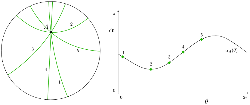
Figure 2: Left diagram: A point $A$ on a time slice of AdS, and five geodesics (in green) that intersect $A$. Right diagram: A point curve $\alpha_{A}(\theta)$ in kinematic space which represents all geodesics that pass through the bulk point $A$. The five diamonds (in green) on the point curve in the right diagram correspond to the five geodesics in the left diagram.

The computation of the total number of RT geodesics passing through a given bulk region is facilitated by the so-called Crofton form $\omega$, which is the volume form on kinematic space. For the kinematic space of the hyperbolic plane, i.e. a time slice of pure AdS, the Crofton form depends only on $\alpha$ (and not on $\theta$) Czech:2015qta

$$\omega=\frac{c}{6\sin^{2}\alpha}d\theta\wedge d\alpha,$$ (13)

where we haven chosen a normalization that is convenient for AdS₃/CFT₂. Using (10) we find that the Crofton form can be written in terms of the second derivative of the entanglement entropy

$$\omega=-\frac{1}{2}\partial_{\alpha}^{2}S(\alpha)d\theta\wedge d\alpha.$$ (14)

Since the Crofton form characterizes the density of geodesics, the length of a bulk curve can now be computed by integrating the Crofton form over the region in kinematic space consisting of all geodesics that intersect the curve. For instance, the geodesic distance or chord length between two points $A$ and $B$ on a bulk time slice is given by the so-called Crofton formula in integral geometry santalo_kac_2004 ; Czech:2015qta

$$\frac{\lambda(A,B)}{4G}=\frac{1}{4}\int_{\Delta_{AB}}\omega(\theta,\alpha).$$ (15)

We have normalized the Crofton form appropriately such that its integral yields the Bekenstein-Hawking entropy. For convex curves it can be easily verified using Stokes’ theorem that the Crofton formula reproduces the differential entropy formula (8) if the Crofton form is given by (14). The integration region $\Delta_{AB}$ in kinematic space is given by the region bounded by the two so-called point curves $\alpha_{A}(\theta)$ and $\alpha_{B}(\theta)$. The point curve of a given point $A$ is the collection of all geodesics that pass through the point $A$, which in kinematic space is a single line $\alpha_{A}(\theta)$ (see figure 2). Thus, the region $\Delta_{AB}$ corresponds in AdS to the set of all geodesics (or RT surfaces) that intersect the geodesic arc between $A$ and $B$ (see figure 6 in the appendices).

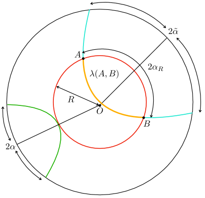
Figure 3: A central circle (in red) of coordinate radius $R$ on a time slice of pure AdS₃. A boundary anchored geodesic (in turquoise) associated to a boundary subregion of size $2\tilde{\alpha}$ intersects the circle at two points $A$ and $B$. The geodesic arc (in orange) between $A$ and $B$ has a bulk angular size $2\alpha_{R}$ and its chord length is denoted by $\lambda(A,B)$. Geodesics (in green) whose turning point is tangent to the circle, satisfy $\alpha_{R}=0$ and $\tilde{\alpha}=\alpha$. The chord length can be formulated as an integral over all geodesics intersecting the arc between $A$ and $B$, and the proper volume of the disk is an integral over geodesics between $\alpha\leq\tilde{\alpha}\leq\pi-\alpha$.

Surprisingly, an explicit derivation of the chord length for pure AdS from the Crofton formula seems to be absent in the literature. For completeness, we have provided this computation in appendix B.2, for the more general case of AdS with a conical defect (which reduces to pure AdS by setting $\gamma=1$). As a result, in vacuum AdS₃ the chord length between two points $A$ and $B$ which lie on a circle of radius $R$ is Abt:2017pmf ; Abt:2018ywl

$$\lambda_{\text{vac}}(\alpha_{R})=L\,\text{arccosh}\!\left[1+2(R/L)^{2}\sin^{2}(\alpha_{R})\right].$$ (16)

Here, $2\alpha_{R}$ is the bulk angle between the points $A$ and $B$ on the circle (see figure 3). These two points lie on a geodesic which is anchored on the asymptotic boundary at the angular coordinates $\theta-\tilde{\alpha}$ and $\theta+\tilde{\alpha}$. The geodesic equation which relates the bulk and boundary opening angles $\alpha_{R}$ and $\tilde{\alpha}$, respectively, takes the form

$$\frac{R}{\sqrt{R^{2}+L^{2}}}\cos\alpha_{R}=\cos\tilde{\alpha}.$$ (17)

We give a derivation of this geodesic equation in appendix B.1, i.e. it follows from the second equation in (195) by setting $r=R$ and $\gamma=1$. One can think of $\alpha_{R}$ as the difference between the bulk angular coordinate $\phi$ and the boundary angular coordinate $\theta$, i.e. $\alpha_{R}=\phi-\theta$. For geodesics which are tangent to the circle we have $\alpha_{R}=0$, and we denote the value of the boundary opening angle by $\alpha$ for such geodesics (see again figure 3). Hence the geodesic equation can also be written as

$$\cos\alpha\,\cos\alpha_{R} =\cos\tilde{\alpha},$$ (18)

$$\text{with}\quad\cos\alpha =\frac{R}{\sqrt{R^{2}+L^{2}}}.$$

The chord length (16) vanishes, of course, for geodesics tangent to the circle, since $\alpha_{R}=0$, and is by definition only non-vanishing for $\tilde{\alpha}\in(\alpha,\pi-\alpha)$. In the rest of the paper we denote generic boundary opening angles by $\tilde{\alpha}$ and we reserve the notation $\alpha$ for CFT intervals whose RT surfaces are tangent to the boundary of a given bulk codimension-one region (like in differential entropy).

Now we can write the bulk volume in terms of the chord length and Crofton form. Recalling that the Crofton form can be interpreted as the density of geodesics, one would expect that the volume of a bulk subregion is proportional to the integral of the chord length times the Crofton form, with an integration region in kinematic space that corresponds to all geodesics intersecting the bulk subregion. By reinstating appropriate normalizations the volume formula in integral geometry reads santalo_kac_2004 ; Abt:2017pmf ; Abt:2018ywl (see also Huang:2019ajv for a similar expression)

$$\frac{V}{4G}=\frac{1}{2\pi}\int_{K}\lambda(\theta^{\prime},\tilde{\alpha}^{\prime})\,\omega(\theta,\tilde{\alpha}),$$ (19)

where $K$ is the set of geodesics that intersect the bulk subregion, and $\lambda$ is the chord length of the intersection of those geodesics and the bulk region (see figure 3).

To gain some intuition for the volume formula, we now compute it explicitly for a circular disk $D$ of coordinate radius $R$ inside a time slice of pure AdS, following Abt:2017pmf . Using equation (14) for the Crofton form in pure AdS and the Ryu-Takayangi formula $S=\ell/(4G),$ we can write the volume formula for a disk as

$$V_{\text{vac}}=-\frac{1}{4\pi}\int_{0}^{2\pi}d\theta\int_{\alpha}^{\pi-\alpha}d\tilde{\alpha}\,\lambda_{\text{vac}}(\theta^{\prime},\tilde{\alpha}^{\prime})\,\partial_{\tilde{\alpha}}^{2}\ell_{\text{vac}}(\tilde{\alpha}),$$ (20)

where the subscript ‘vac’ signifies that the chord length $\lambda$ of a geodesic arc and the length $\ell$ of a boundary anchored geodesic are evaluated in vacuum AdS. For computational purposes it is convenient to replace the integral over $\tilde{\alpha}$ by an integral over $\alpha_{R}$, based on the identity

$$\partial^{2}_{\tilde{\alpha}}\ell_{\text{vac}}(\tilde{\alpha})\,d\tilde{\alpha}=\partial^{2}_{\alpha_{R}}\lambda_{\text{vac}}(\alpha_{R})\,d\alpha_{R}\,,$$ (21)

which can be checked using the equations (10) and (16). The volume formula then becomes

$$V_{\text{vac}} =-\frac{1}{4\pi}\int_{0}^{2\pi}d\theta\int_{0}^{\pi}d\alpha_{R}\,\lambda_{\text{vac}}\,\partial^{2}_{\alpha_{R}}\lambda_{\text{vac}}=\frac{1}{2}\int_{0}^{\pi}d\alpha_{R}\left(\partial_{\alpha_{R}}\lambda_{\text{vac}}\right)^{2}$$ (22)

$$=\int_{0}^{\pi}d\alpha_{R}\frac{2R^{2}\cos^{2}(\alpha_{R})}{1+(R/L)^{2}\sin^{2}(\alpha_{R})}=2\pi L^{2}\left(\sqrt{1+(R/L)^{2}}-1\right).$$

This reproduces the proper volume of a disk in pure AdS. In the second equality on the first line we performed the trivial integral over $\theta$ and we partially integrated, noting that the boundary term vanishes since $\lambda_{\text{vac}}=0$ at $\alpha_{R}=0,\pi$.

The volume formula (19) actually holds for an arbitrary bulk subregion in pure AdS, as shown in Abt:2018ywl . Similarly, it applies to bulk subregions in quotient spaces of pure AdS₃, since the kinematic space for these geometries can be obtained from quotients of the kinematic space for pure AdS Abt:2018ywl ; Cresswell:2017mbk . The Crofton form follows from the quotient procedure and still takes the form (14) for time slices of static quotient spaces. Next we repeat the computation above for a disk in the quotient space of AdS₃ with a conical defect.

The volume formula for a disk in the conical AdS spacetime is similar to the expression (20) for pure AdS, except that the integration region now depends on the defect parameter $\gamma$

$$V_{\text{con}}=-\frac{1}{4\pi}\int_{0}^{2\pi}d\theta\int_{\alpha}^{\pi/\gamma-\alpha}d\tilde{\alpha}\,\lambda_{\text{con}}(\theta^{\prime},\tilde{\alpha}^{\prime})\partial_{\tilde{\alpha}}^{2}\ell_{\text{con}}(\tilde{\alpha}).$$ (23)

The chord length for the conical defect spacetime (6) is computed in appendix B.2 in two different ways, using the embedding space formalism and the kinematic space formalism. The result is

$$\lambda_{\text{con}}(\alpha_{R})=L\text{arccosh}\left[1+2R^{2}/(\gamma L)^{2}\sin^{2}(\gamma\alpha_{R})\right],$$ (24)

where $\alpha_{R}$ is the bulk opening angle between two points on a circle of radius $R$ (see figure 3). These two points lie on a boundary anchored geodesic, with boundary opening angle $\tilde{\alpha}$, for which the geodesic equation reads (see appendix B.1 for a derivation)

$$\cos(\gamma\alpha)\,\cos(\gamma\alpha_{R}) =\cos(\gamma\tilde{\alpha}).$$ (25)

Here, $\alpha$ is the value of the boundary opening angle $\tilde{\alpha}$ for which the boundary anchored (Ryu-Takayanagi) geodesic is tangent to the circle of radius $R$, i.e. $\alpha_{R}=0$, satisfying

$$\cos(\gamma\alpha)=\frac{R}{\sqrt{R^{2}+\gamma^{2}L^{2}}}\qquad\text{or}\qquad R=L\gamma\cot(\gamma\alpha).$$ (26)

We now compute the volume of a disk in conical AdS using the chord length. In equation (23) we can replace the integral over $\tilde{\alpha}$ by an integral over $\alpha_{R}$ using

$$\partial^{2}_{\tilde{\alpha}}\ell_{\text{con}}(\tilde{\alpha})\,d\tilde{\alpha}=\partial^{2}_{\alpha_{R}}\lambda_{\text{con}}(\alpha_{R})\,d\alpha_{R}\,.$$ (27)

This can be seen geometrically from figure 3, but it can also be explicitly checked from (24) and (48). After inserting this and performing the trivial integral over $\theta$, the volume formula reduces to a single integral over $\alpha_{R}$

$$V_{\text{con}} =-\frac{1}{2}\int_{0}^{\pi/\gamma}d\alpha_{R}\,\lambda_{\text{con}}\partial^{2}_{\alpha_{R}}\lambda_{\text{con}}=\frac{1}{2}\int_{0}^{\pi/\gamma}d\alpha_{R}(\partial_{\alpha_{R}}\lambda_{\text{con}})^{2}$$ (28)

$$=\int_{0}^{\pi/\gamma}d\alpha_{R}\,\frac{2R^{2}\cos^{2}(\gamma\alpha_{R})}{1+R^{2}/(\gamma L)^{2}\sin^{2}(\gamma\alpha_{R})}=2\pi L^{2}\left(\sqrt{\gamma^{2}+(R/L)^{2}}-\gamma\right).$$

In the second equality we integrated by parts and removed the boundary term, since $\lambda_{\text{con}}=0$ at $\alpha_{R}=0,\pi/\gamma.$ The final expression is indeed the volume of a disk in conical AdS.

2.1.3 Boundary dual of finite bulk volume

In this section we discuss the CFT₂ dual of the volume of a subregion inside a time slice of pure AdS₃ (or a static quotient space of AdS₃). The volume formula (19) can be expressed in terms of entanglement entropies, using the Crofton formula (15) and equation (14) for the Crofton form of the hyperbolic plane,

$$V=\frac{G^{2}}{2\pi}\int_{K}d\theta\,d\tilde{\alpha}\int_{\Delta_{AB}}d\theta^{\prime}\,d\tilde{\alpha}^{\prime}\,\partial_{\tilde{\alpha}}^{2}\,S(\tilde{\alpha})\,\partial_{\tilde{\alpha}^{\prime}}^{2}\,S(\tilde{\alpha}^{\prime}).$$ (29)

Clearly, the right-hand side is not a CFT quantity, as it still involves Newton’s constant $G$. However, we can define a manifestly field theoretic quantity by dividing the volume by an appropriate dimensionful factor. Following the ‘complexity=volume’ proposal Susskind:2014moa ; Brown:2015bva we divide the volume by $GL$, where $L$ is the AdS radius, and we call the resulting dimensionless quantity holographic complexity

$$\mathcal{C}=\frac{V}{4GL}.$$ (30)

The factor $1/4$ is conveniently chosen since the same factor appears in differential entropy. The dimensionful proportionality factor $1/(GL)$ has been used in earlier definitions of holographic complexity for boundary thermofield double states Susskind:2014moa and for boundary subregion density matrices Alishahiha:2015rta ; Carmi:2016wjl . This is also the same factor that connects boundary Fisher information and bulk volume Banerjee:2017qti ; Sarkar:2017pjp . As a result, we find the following definition of the boundary dual of the bulk volume

$$\mathcal{C}=\frac{3}{16\pi c}\int_{K}d\theta\,d\tilde{\alpha}\int_{\Delta_{AB}}d\theta^{\prime}\,d\tilde{\alpha}^{\prime}\,\partial_{\tilde{\alpha}}^{2}\,S(\tilde{\alpha})\,\partial_{\tilde{\alpha}^{\prime}}^{2}\,S(\tilde{\alpha}^{\prime}),$$ (31)

where we employed $c=3L/(2G).$ This is a pure CFT quantity, since the regions $K$ and $\Delta_{AB}$ in kinematic space can be defined in terms of boundary coordinates $(\theta,\tilde{\alpha})$ (see also section 2.2.2). The information theoretic interpretation of this expression is not clear to us, but at least it provides a precise dictionary between the bulk volume and a boundary integral over entanglement entropies. This dictionary is our second input for the boundary interpretation of the bulk first law (differential entropy being the first input).

Regarding the complexity interpretation of the bulk volume, the CFT quantity could be defined as the complexity of a global state on a time slice in the CFT, where a UV cutoff has been implemented in the theory. The cutoff scale is related to the boundary of a bulk subregion in a time slice of AdS through the UV/IR correspondence Susskind:1998dq ; Peet:1998wn (the CFT time slice coincides with the asymptotic boundary of the bulk time slice). If the bulk subregion is a central disk of a fixed radius, then the CFT lives at a radial cutoff in AdS. It would be interesting to make this proposal for cutoff complexity more precise, see for example the recent paper Chen:2020nlj .

We should be careful in distinguishing this notion of cutoff complexity from the usual notion of subregion complexity Alishahiha:2015rta ; Carmi:2016wjl . The latter is argued to be the complexity of a reduced density matrix associated to a boundary subregion, dual to the volume of the extremal bulk codimension-one region bounded by the boundary subregion and the associated RT surface (or dual to the action of the Wheeler-deWitt patch of the bulk region). Cutoff complexity depends on the global state of a time slice of the CFT, or on the reduced state associated to a time strip, whereas subregion complexity is a property of a reduced density matrix associated to a subregion. The two definitions are only equivalent in the limit where the boundary subregion coincides with the entire time slice in the CFT. The cutoff complexity and subregion complexity are in that case dual to the volume of an extremal time slice of AdS, which can be regularized by choosing an IR cutoff in the bulk which matches the UV cutoff on the boundary. We discuss this limit further in section 2.3.

Note that the complexity=volume proposal (30) differs from the holographic dictionary in Abt:2017pmf ; Abt:2018ywl . In particular, their definition of topological complexity $\mathcal{C}_{\text{top}}$ for a bulk subregion $\Sigma$ of constant intrinsic scalar curvature $\mathcal{R}$ is given by

$$\mathcal{C}_{\text{top}}=-\frac{1}{2}\int_{\Sigma}dV\mathcal{R}=\frac{V_{\Sigma}}{L^{2}}.$$ (32)

In the last step, we inserted the expression $\mathcal{R}=-2/L^{2}$, which holds for time slices of AdS₃. In terms of entanglement entropy the topological complexity reads

$$\mathcal{C}_{\text{top}}=\frac{9}{8\pi c^{2}}\int_{K}d\theta\,d\tilde{\alpha}\int_{\Delta_{AB}}d\theta^{\prime}\,d\tilde{\alpha}^{\prime}\,\partial_{\tilde{\alpha}}^{2}\,S(\tilde{\alpha})\,\partial_{\tilde{\alpha}^{\prime}}^{2}\,S(\tilde{\alpha}^{\prime}).$$ (33)

Note that $C_{\text{top}}$ does not depend on the central charge, because the $1/c^{2}$ cancels against the central charges in the two factors of the entanglement entropy $S\sim c$ (at least for the vacuum). The region $\Sigma$ is often taken to be the codimension-one region bounded by the RT surface and a boundary interval, but the expression above applies to any bulk subregion (since the volume formula applies to arbitrary regions). The motivation for considering this definition comes from the Gauss-Bonnet theorem, where the integral in (32) term appears as being associated with the volume of the region. Through the Gauss-Bonnet theorem the resulting complexity is related to the Euler number of the bulk subregion, cf. equation (96), manifesting the topological nature of the definition. Both proposals for holographic complexity (30) and (32) are valid dimensionless CFT quantities, but we work with the first proposal in the rest of the paper for three reasons: a) it is more widely used in the literature, b) it is proportional to the central charge like differential entropy, and c) it is well defined in higher dimensions (see the comment below equation (159)).

2.2 First law of differential entropy and holographic complexity

In this section we derive a CFT₂ counterpart of the first law of causal diamonds in AdS₃. The CFT first law involves a variation of the differential entropy and holographic complexity, which are respectively dual to (the variation of) the area and volume of a disk in AdS. We proceed in deriving the boundary relation by first computing the variations of $S_{\text{diff}}$ and $\mathcal{C}$ separately in the CFT, and then combining them into one variational identity. We consider three independent types of variations in the CFT: 1) a variation of the boundary subregion size $\alpha$ in a fixed coordinate system, 2) a variation of the scaling dimension $\Delta$ of operators acting on the vacuum state, and 3) a variation of the central charge $c$ in the space of CFTs. While studying one particular variation, we keep the other two quantities fixed. Both differential entropy and holographic complexity change under the variations of $(\alpha,\Delta,c)$. A particular combination of $\delta S_{\text{diff}}$ and $\delta\mathcal{C}$ yields a new variational relation, which for brevity we call the ‘first law of differential entropy’. One can think of this as a dynamical constraint that any $2d$ holographic field theory must satisfy.

For the most part, we assume the central charge to be large such that the holographic dual has a classical geometry. Further, we mostly consider those state variations in the CFT which are dual to the creation of a conical defect in AdS. In other words, we take the perturbed geometry in the bulk (after a metric perturbation of pure AdS₃) to be the classical spacetime which is locally identical to AdS₃ but globally has an angular deficit (see section 3.1). A conical defect spacetime with angular periodicity $2\pi/N$ corresponds to the quotient space AdS${}_{3}/\mathbb{Z}_{N}$, with $N$ a positive integer. A conical defect in AdS is dual to an excited state created, via the state/operator correspondence, by a heavy operator in the CFT Balasubramanian:1999zv ; Balasubramanian:2000rt ; Krasnov:2000ia ; Lunin:2002bj . There is substantial evidence that the CFT state dual to AdS${}_{3}/\mathbb{Z}_{N}$ is excited by an operator which, at large $c$, has scaling dimension Benjamin:2020mfz ; Asplund:2014coa ; Cresswell:2018mpj

$$\Delta=\frac{c}{12}\left(1-\frac{1}{N^{2}}\right)+\mathcal{O}(c^{0}).$$ (34)

The leading-order term is the scaling dimension of a twist operator Dixon:1986qv ; Knizhnik ; Calabrese:2009qy . At the orbifold point of the D1-D5 CFT the dual of AdS${}_{3}/\mathbb{Z}_{N}$ has indeed been identified as the state created by acting with a twist field on the vacuum Lunin:2000yv ; Martinec:2001cf ; Balasubramanian:2014sra . Taking subleading corrections into account in $\Delta$ is equivalent to including perturbative quantum corrections in the bulk stress-energy tensor, due to the presence of quantum fields in a fixed AdS background. In the following we neglect these subleading $1/c$ corrections and we only consider CFT excited states with large $\Delta$ dual to a classical geometry with a point particle.

In terms of the conical defect parameters $\gamma=1/N$ and $\epsilon=1-\gamma$, which we often use, the scaling dimension to leading order reads

$$\Delta=\frac{c}{12}\left(1-\gamma^{2}\right)=\frac{c}{6}\epsilon-\frac{c}{12}\epsilon^{2}.$$ (35)

For first-order variations around the vacuum state we thus have

$$\delta\Delta=\frac{c}{6}\delta\epsilon.$$ (36)

Note that $\delta\Delta=\Delta$ and $\delta\epsilon=\epsilon$, as the vacuum state corresponds to $\Delta=0$ and $\epsilon=0$.

2.2.1 Varying differential entropy

The change in differential entropy under the variation of the subregion size $\alpha$, scaling dimension $\Delta$ and central charge $c$ is

$$\delta S_{\text{diff}}=\delta_{\alpha}S_{\text{diff}}\big{|}_{\Delta,c}+\delta_{\Delta}S_{\text{diff}}\big{|}_{\alpha,c}+\delta_{c}S_{\text{diff}}\big{|}_{\alpha,\Delta}.$$ (37)

Note that if $\Delta$ is kept fixed, we should evaluate the differential entropy in the ground state of CFT. The variation $\delta_{\Delta}$ in the second term denotes a state variation induced by acting with an operator of dimension $\Delta$ on the vacuum. We start with computing the second term using two different methods, and afterwards we discuss the other terms.

Method 1) Since differential entropy (8) is expressed in terms of the entanglement entropy $S(\alpha)$, we can employ the first law of entanglement to calculate the change in differential entropy under a state variation. Recall that the reduced density matrix associated to a subregion can be expressed as

$$\rho={e^{-H_{\text{mod}}}\over Z},$$ (38)

where $H_{\text{mod}}$ is the so-called modular Hamiltonian. Under a variation of the state of the system, it follows that the variation of the entanglement entropy is equal to the variation of the expectation value of $H_{\text{mod}}$ Blanco:2013joa ; Wong:2013gua

$$\delta_{\Delta}S=\delta_{\Delta}\!\left<H_{\text{mod}}\right>.$$ (39)

This is the first law of entanglement. In order to derive a first law for differential entropy, we differentiate with respect to $\alpha$ on both sides and then take the integral over $\theta$:

$$\frac{1}{2}\int^{2\pi}_{0}d\theta\,\frac{d}{d\alpha}\delta_{\Delta}S(\alpha)\Big{|}_{\alpha(\theta)}=\frac{1}{2}\int^{2\pi}_{0}d\theta\,\frac{d}{d\alpha}\,\delta_{\Delta}\!\left<H_{\text{mod}}\right>\Big{|}_{\alpha(\theta)}.$$ (40)

The left-hand side is, of course, the state variation of the differential entropy. The challenge lies in understanding the right-hand side of this equation. In order to do so, we use the fact that the modular Hamiltonian for the reduced density matrix of the CFT global vacuum state restricted to a ball-shaped region $B$ can be interpreted as a conserved charge Casini:2011kv

$$H_{\text{mod}}=\int_{B}d\Sigma^{\mu}\,\xi^{\nu}\,T_{\mu\nu}=L\int_{\theta-\alpha}^{\theta+\alpha}d\bar{\theta}\,\xi^{t}_{(\theta,\alpha)}(\bar{\theta})\,T_{tt}(\bar{\theta})\Big{|}_{t=0}.$$ (41)

Here $\Sigma^{\mu}$ and $T_{\mu\nu}$ are, respectively, the volume-form on the subregion and the CFT stress-energy tensor. The curvature radius $L$ appears due to the square root of the determinant of the metric (7) on the boundary cylinder. Further, $\xi^{t}_{(\theta,\alpha)}$ is the time component of the conformal Killing vector that generates a flow which remains inside the past and future domain of dependence (a.k.a. the causal diamond) of the ball-shaped subregion. Since the two-dimensional CFT lives on a cylinder in our setup, the spherical subregion is an interval with angular size $2\alpha$ and center at $\bar{\theta}=\theta$, and we assume it lies inside the $t=0$ time slice. In appendix C we provide a derivation of the conformal Killing vector $\xi$ generating the conformal isometry that preserves a causal diamond on the cylinder, both from a boundary and a bulk perspective.

By plugging in the expression above for the modular Hamiltonian into (40) and taking the derivative with respect to $\alpha$ inside the $\bar{\theta}$-integral – this is allowed since $\xi_{(\theta,\alpha)}=0$ at the boundary values of the integral, i.e. at $t=0$ and $\bar{\theta}=\theta\pm\alpha$, which are the edges of the diamond – one finds

$$\delta_{\Delta}S_{\text{diff}}\big{|}_{\alpha,c}=\frac{1}{2}L\int^{2\pi}_{0}d\theta\int_{\theta-\alpha}^{\theta+\alpha}d\bar{\theta}\,\frac{d}{d\alpha}\,\xi^{t}_{(\theta,\alpha)}(\bar{\theta})\delta_{\Delta}\!\left<T_{tt}(\bar{\theta})\right>\Big{|}_{t=0}.$$ (42)

We can interchange the order of the integrals by imposing $|\bar{\theta}-\theta|\leq\alpha$. This gives

$$\delta_{\Delta}S_{\text{diff}}\big{|}_{\alpha,c}=\frac{1}{2}L\int^{2\pi}_{0}d\bar{\theta}\int_{\bar{\theta}-\alpha}^{\bar{\theta}+\alpha}d\theta\,\frac{d}{d\alpha}\,\xi^{t}_{(\theta,\alpha)}(\bar{\theta})\delta_{\Delta}\!\left<T_{tt}(\bar{\theta})\right>\Big{|}_{t=0}.$$ (43)

Lastly, we insert the conformal Killing vector whose flow preserves a causal diamond on the boundary cylinder and has unit surface gravity

$$\xi_{(\theta,\alpha)}(\bar{\theta})=\frac{1}{\sin\alpha}\left[\left(\cos(t/L)\cos(\bar{\theta}-\theta)-\cos\alpha\right)\!L\partial_{t}-\sin(t/L)\sin(\bar{\theta}-\theta)\partial_{\bar{\theta}}\right].$$ (44)

This vector field vanishes at the edges of the diamond $\{t=0,\bar{\theta}=\theta\pm\alpha\}$ and the past and future vertices $\{t/L=\pm\alpha,\bar{\theta}=\theta\}$, and acts as a null flow on the null boundaries of the diamond $\{t/L+\bar{\theta}=\theta\pm\alpha;t/L-\bar{\theta}=-\theta\pm\alpha\}$. The derivative of the time component of this vector with respect to $\alpha$, evaluated at $t=0$, is

$$\frac{d}{d\alpha}\xi^{t}_{({{\theta}},\alpha)}\Big{|}_{t=0}=L\left[1-\frac{\cos\alpha}{\sin^{2}\alpha}\left(\cos(\bar{\theta}-\theta)-\cos\alpha\right)\right].$$ (45)

After evaluating the inner ${\theta}$-integral we find

$$\delta_{\Delta}S_{\text{diff}}\big{|}_{\alpha,c} =L^{2}\int_{0}^{2\pi}d\bar{\theta}\left(-\frac{\cos\alpha}{\sin\alpha}+\frac{\alpha}{\sin^{2}\alpha}\right)\delta_{\Delta}\!\left<T_{tt}(\bar{\theta})\right>$$ (46)

$$=2\pi\left(-\frac{\cos\alpha}{\sin\alpha}+\frac{\alpha}{\sin^{2}\alpha}\right)\delta\Delta,$$

where in the last line we assumed $\alpha\neq\alpha(\bar{\theta})$, which corresponds to a spherical region in AdS₃, and we inserted the relationship between the stress-energy tensor expectation value and the scaling dimension

$$L^{2}\int_{0}^{2\pi}d\bar{\theta}\,\delta_{\Delta}\langle T_{tt}(\bar{\theta})\rangle=2\pi\delta\Delta.$$ (47)

Method 2) Note that the derivation above holds for arbitrary state perturbations and for arbitrary boundary subregions $\alpha(\bar{\theta})$, until the first line of (46), corresponding to arbitrary bulk regions. However, if the perturbed state is dual to a conical defect in AdS₃, and if $\alpha$ is constant, there is an alternate method of obtaining the state variation of differential entropy. In particular, we can compute the state variation by subtracting the differential entropy for the vacuum state from the differential entropy for the excited state dual to the conical defect spacetime. To do so, we need the entanglement entropy for the excited state dual to a conical defect spacetime Balasubramanian:2014sra ; Asplund:2014coa ; Visser2

$$S^{\text{con}}(\alpha)=\frac{c}{3}\log\left[\frac{2L}{\mu\gamma}\sin(\gamma\alpha)\right].$$ (48)

The variation in differential entropy is now equal to the difference between the differential entropy for the excited state dual to the conical defect space and the differential entropy for the vacuum state

$$\delta_{\Delta}S_{\text{diff}}\big{|}_{\alpha,c} =\frac{1}{2}\int_{0}^{2\pi}d\theta\frac{d}{d\alpha}S^{\text{con}}(\alpha)-\frac{1}{2}\int_{0}^{2\pi}d\theta\frac{d}{d\alpha}S^{\text{vac}}(\alpha)$$ (49)

$$=\frac{1}{2}\int_{0}^{2\pi}d\theta\,\frac{c}{3}\,\left[(1-\epsilon)\,\frac{\cos\left[(1-\epsilon)\alpha\right]}{\sin\left[(1-\epsilon)\alpha\right]}-\frac{\cos\alpha}{\sin\alpha}\right]$$

$$=2\pi\left(-\frac{\cos\alpha}{\sin\alpha}+\frac{\alpha}{\sin^{2}\alpha}\right)\frac{c}{6}\,\epsilon+\mathcal{O}(\epsilon^{2}).$$

This is the same result as (46), since $\delta\Delta=(c/6)\epsilon$ up to first order in $\epsilon$, cf. equation (36).

After dealing with the state variation, we can now concentrate on the first and third term in (37), i.e. the variation of the subregion size and central charge, respectively. The change in differential entropy under an $\alpha$ variation, at fixed $\Delta$ and $c$, is to first order

$$\delta_{\alpha}S_{\text{diff}}\big{|}_{\Delta,c}=\frac{\partial S_{\text{diff}}^{\text{vac}}}{\partial\alpha}\delta\alpha=-\frac{\pi c}{3}\frac{1}{\sin^{2}\alpha}\delta\alpha,$$ (50)

where we used the expression (11) for the vacuum differential entropy with $\alpha\neq\alpha(\theta)$. Similarly, the differential entropy variation due to a variation of the central charge, at fixed $\alpha$ and $\Delta$, is

$$\delta_{c}S_{\text{diff}}\big{|}_{\alpha,\Delta}=\frac{\partial S_{\text{diff}}^{\text{vac}}}{\partial c}\,\delta c=\frac{1}{c}\,S_{\text{diff}}^{\text{vac}}\,\delta c=\frac{\pi}{3}\frac{\cos\alpha}{\sin\alpha}\delta c.$$ (51)

Finally, combining the variations (46), (50) and (51), we find that the total differential entropy variation is to first order given by

$$\delta S_{\text{diff}} =\frac{\pi}{3}\frac{\cos\alpha}{\sin\alpha}\delta c-\frac{\pi c}{3}\frac{1}{\sin^{2}\alpha}\delta\alpha+2\pi\left(-\frac{\cos\alpha}{\sin\alpha}+\frac{\alpha}{\sin^{2}\alpha}\right)\delta\Delta.$$ (52)

2.2.2 Varying holographic complexity

Our next task is to study the change in holographic complexity (30) due to $\alpha$, $\Delta$, and $c$ variations

$$\delta\mathcal{C}=\delta_{\alpha}\,\mathcal{C}\big{|}_{\Delta,c}+\delta_{\Delta}\,\mathcal{C}\big{|}_{\alpha,c}+\delta_{c}\,\mathcal{C}\big{|}_{\alpha,\Delta}.$$ (53)

We start with computing the second term, i.e. the state variation of holographic complexity at fixed $\alpha$ and $c$. Unfortunately, unlike with the differential entropy variation, we cannot use the first law of entanglement in this case, since the volume formula (19), on which our holographic complexity is based, applies only to locally AdS₃ spacetimes. This means that the holographic complexity formula (31) holds for CFT states which are dual to quotients of AdS₃, such as the conical defect spacetime and the BTZ black hole, but does not apply to arbitrary variations of the vacuum state. In particular, it does not hold for small deviations from the vacuum state, i.e. with $\Delta\ll c$, dual to geometries with small local variations away from pure AdS₃ Abt:2018ywl .

Therefore, we use the second method in the previous section to determine the complexity variation. That means we define the complexity state variation as the difference between the complexity for the excited state dual to conical AdS and the complexity for the vacuum

$$\delta_{\Delta}\mathcal{C}\big{|}_{{\alpha},c}:=\left(\mathcal{C}_{\text{con}}-\mathcal{C}_{\text{vac}}\right)\Big{|}_{\alpha,c}.$$ (54)

The holographic complexity for both states could in principle be computed by inserting the entanglement entropies for the vacuum and excited state, i.e. (10) and (48) respectively, into the definition (31) (see Abt:2018ywl for similar computations). However, we find it computationally easier to express the complexity first in terms of the chord length, instead of the entanglement entropy. Following the steps in (22) we can write the complexity for the vacuum state as

$$\mathcal{C}_{\text{vac}}=\frac{c}{12}\int_{0}^{\pi}d\alpha_{R}\,(\partial_{\alpha_{R}}\tilde{\lambda}_{\text{vac}})^{2}.$$ (55)

Here $\tilde{\lambda}_{\text{vac}}=\lambda_{\text{vac}}/L$ is the dimensionless chord length for the vacuum state, given in (16). Although the chord length is a bulk quantity, defined as the length of a geodesic arc, it can also be interpreted as a boundary quantity. By writing the bulk opening angle $\alpha_{R}$ and the radius $R$ in terms of the boundary opening angles $\alpha$ and $\tilde{\alpha}$, using (17) and (18), we find a boundary expression for the vacuum chord length

$$\tilde{\lambda}_{\text{vac}}(\tilde{\alpha})=\text{arccosh}\left[1+2\frac{\cos^{2}\alpha-\cos^{2}\tilde{\alpha}}{\sin^{2}\alpha}\right].$$ (56)

Notice that this is only a function of $\tilde{\alpha}$, the angle $\alpha$ determines the size of the disk in the bulk and is hence fixed in the computation of the volume formula. The vacuum complexity can be derived by plugging this expression for the chord length into (55) and, after a change of variables, performing the integral over $\tilde{\alpha}$ (or, equivalently, inserting equation (16) for the chord length and integrating over $\alpha_{R}$)

$$\mathcal{C}_{\text{vac}}=\frac{\pi c}{3}\left(\frac{1}{\sin\alpha}-1\right).$$ (57)

Note that, unlike entanglement entropy (10), the complexity and differential entropy of the vacuum state are independent of the UV cutoff $\mu$ of the CFT.

Next, we turn to the complexity of the CFT state dual to conical AdS (see also Ageev:2018nye ). We compute the holographic complexity through the volume formula, which can be expressed entirely in terms of the chord length, cf. equation (28), in a similar way as for pure AdS,

$$\mathcal{C}_{\text{con}}=\frac{c}{12}\int_{0}^{\pi/\gamma}d\alpha_{R}\,(\partial_{\alpha_{R}}\tilde{\lambda}_{\text{con}})^{2}.$$ (58)

By changing variables we replace the integral over $\alpha_{R}$ by an integral over $\tilde{\alpha}$, and we write the dimensionless chord length $\tilde{\lambda}_{\text{con}}=\lambda_{\text{con}}/L$ as a boundary quantity, using (25) and (26),

$$\tilde{\lambda}_{\text{con}}(\tilde{\alpha})=\text{arccosh}\left[1+2\frac{\cos^{2}(\gamma\alpha)-\cos^{2}(\gamma\tilde{\alpha})}{\sin^{2}(\gamma\alpha)}\right].$$ (59)

This means that the complexity formula (58) can be written purely in terms of CFT quantities. Performing the remaining integral over $\tilde{\alpha}$ (or, equivalently, over $\alpha_{R}$), the complexity for CFT states dual to conical AdS turns out to be

$$\mathcal{C}_{\text{con}}=\frac{\pi c}{3}\gamma\left(\frac{1}{\sin(\gamma\alpha)}-1\right).$$ (60)

Expanded to first order in $\epsilon=1-\gamma$, the complexity is given by

$$\mathcal{C}_{\text{con}}=\frac{\pi c}{3}\left[\frac{1}{\sin\alpha}-1+\left(\frac{\alpha\cos\alpha}{\sin^{2}\alpha}-\frac{1}{\sin\alpha}+1\right)\epsilon+\mathcal{O}(\epsilon^{2})\right].$$ (61)

Thus, the state variation of the complexity is to first order

$$\delta_{\Delta}\mathcal{C}\big{|}_{\alpha,c}=2\pi\left(\frac{\alpha\cos\alpha}{\sin^{2}\alpha}-\frac{1}{\sin\alpha}+1\right)\delta\Delta,$$ (62)

where we have used (36) to replace $\delta\epsilon$ by $\delta\Delta$.

Finally, we turn to the $\alpha$ and $c$ variations of holographic complexity. As the state is unchanged in both variations we can directly use equation (57) for the vacuum complexity and take partial derivatives with respect to $\alpha$ and $c$. We end up with the following first-order variations

$$\delta_{\alpha}\mathcal{C}\big{|}_{\Delta,c}=\frac{\partial\mathcal{C}_{\text{vac}}}{\partial\alpha}\delta\alpha=-\frac{\pi c}{3}\frac{\cos\alpha}{\sin^{2}\alpha}\delta\alpha,$$ (63)

and

$$\delta_{c}\,\mathcal{C}\big{|}_{\alpha,\Delta}=\frac{\partial\mathcal{C}_{\text{vac}}}{\partial c}\delta c=\frac{1}{c}\,\mathcal{C}_{\text{vac}}\,\delta c=\frac{\pi}{3}\left(\frac{1}{\sin\alpha}-1\right)\delta c.$$ (64)

Thus, the total complexity variation is

$$\delta\mathcal{C}=\frac{\pi}{3}\left(\frac{1}{\sin\alpha}-1\right)\delta c-\frac{\pi c}{3}\frac{\cos\alpha}{\sin^{2}\alpha}\delta\alpha+2\pi\left(\frac{\alpha\cos\alpha}{\sin^{2}\alpha}-\frac{1}{\sin\alpha}+1\right)\delta\Delta.$$ (65)

2.2.3 Combining the variations

At this point, we are ready to write down a first law in CFT₂ involving the change in differential entropy and complexity under the variations of $\alpha$, $\Delta$ and $c$. We proceed by computing a particular combination of variations of differential entropy and complexity,

$$\delta S_{\text{diff}}-\left(\frac{\partial S_{\text{diff}}}{\partial\mathcal{C}}\right)_{c}\,\delta\mathcal{C},$$ (66)

since such a combination typically appears in a thermodynamic relation. To be specific, if the internal energy depends on the three equilibrium state variables $S_{\text{diff}}$, $\mathcal{C}$ and $c$, i.e. $E=E(S_{\text{diff}},\mathcal{C},c)$, then its variation is by definition equal to

$$\delta E=\left(\frac{\partial E}{\partial S_{\text{diff}}}\right)_{\mathcal{C},c}\!\!\delta S_{\text{diff}}+\left(\frac{\partial E}{\partial\mathcal{C}}\right)_{S_{\text{diff}},c}\!\!\delta\mathcal{C}+\left(\frac{\partial E}{\partial c}\right)_{S_{\text{diff}},\mathcal{C}}\!\!\delta c.$$ (67)

This can be written in a different form using Maxwell’s relation

$$\delta E=\left(\frac{\partial E}{\partial S_{\text{diff}}}\right)_{\mathcal{C},c}\!\!\left(\delta S_{\text{diff}}-\left(\frac{\partial S_{\text{diff}}}{\partial\mathcal{C}}\right)_{E,c}\!\!\delta\mathcal{C}\right)+\left(\frac{\partial E}{\partial c}\right)_{S_{\text{diff}},\mathcal{C}}\!\!\delta c.$$ (68)

We find that the combination of variations (66) indeed appears in the variation of the internal energy.

Another motivation for studying the particular combination of variations (66) is that it corresponds to $\delta(A/4G)-kL\delta(V/4GL)$ in the dual AdS spacetime, where $k$ is the trace of the extrinsic curvature of the boundary of the disk as embedded in the disk. The first law of causal diamonds can be expressed in terms of this combination of area and volume variations, as we will show in section 4. Hence, we expect that the combination of variations (66) appears in the dual boundary first law. The partial derivative of $S_{\text{diff}}$ with respect to $\mathcal{C}$ should be evaluated in the vacuum, at fixed central charge, and can be easily calculated as

$$\left(\frac{\partial S_{\text{diff}}^{\text{vac}}}{\partial\mathcal{C}_{\text{vac}}}\right)_{c}=\frac{\partial S_{\text{diff}}^{\text{vac}}}{\partial\alpha}\left(\frac{\partial\mathcal{C}_{\text{vac}}}{\partial\alpha}\right)^{-1}=-\frac{\pi c}{3}\frac{1}{\sin^{2}\alpha}\left(-\frac{\pi c}{3}\frac{\cos\alpha}{\sin^{2}\alpha}\right)^{-1}=\frac{1}{\cos\alpha}.$$ (69)

In the bulk this is dual to the product of the extrinsic trace $k$ and the AdS radius $L$, i.e. $kL=1/\cos\alpha$, cf. equation (141).

We can now compute the combination of variations of differential entropy and complexity separately for $\alpha,\Delta$ and $c$ induced variations. Firstly, for variations which change the subregion size $\alpha$, but keep $\Delta$ and $c$ fixed, the combination vanishes to first order

$$\left(\delta_{\alpha}S_{\text{diff}}-\frac{1}{\cos\alpha}\,\delta_{\alpha}\mathcal{C}\right)_{\Delta,c}=0.$$ (70)

This follows directly from the $\alpha$ variations of differential entropy and complexity, (50) and (63) respectively. Note that the choice of relative coefficient (69) is crucial for the cancellations between the two variations. The $\alpha$ variation is an example of a global conformal transformation in the CFT, in particular a dilatation, hence it is dual to a bulk isometry transformation. In Jacobson:2018ahi it has been shown that the combination $\delta_{\chi}A-k\delta_{\chi}V$ vanishes for variations of ball-shaped regions in AdS with vanishing extrinsic curvature induced by arbitrary diffeomorphisms $\chi$, in particular it is zero for variations induced by isometries. Hence, from the AdS/CFT duality we expect that (66) vanishes for variations induced by arbitrary global conformal transformations (since they are dual to isometries in the bulk), not just for $\alpha$ variations, but we do not have a proof of this in the CFT.

Secondly, under a small change in $\Delta$, at fixed $\alpha$ and $c$, the combination of variations becomes

$$\left(\delta_{\Delta}S_{\text{diff}}-\frac{1}{\cos\alpha}\delta_{\Delta}\mathcal{C}\right)_{\alpha,c}=-2\pi\left(\frac{1}{\cos\alpha}-\frac{\sin\alpha}{\cos\alpha}\right)\delta\Delta.$$ (71)

This can be derived by inserting the state variations of differential entropy and complexity. The state variation of differential entropy (46) is valid for arbitrary perturbations, but the variation of complexity (62) is specific for first-order variations from the vacuum state to the excited state dual to conical AdS. It would be interesting to see whether the equality above holds more generally for arbitrary first order perturbations of the vacuum state.

Furthermore, under the variation of the central charge, at fixed $\alpha$ and $\Delta$, the combination of variations takes a very simple form

$$\left(\delta_{c}S_{\text{diff}}-\frac{1}{\cos\alpha}\delta_{c}\mathcal{C}\right)_{\alpha,\Delta}=\left(S_{\text{diff}}^{\text{vac}}-\frac{1}{\cos\alpha}\mathcal{C}_{\text{vac}}\right)\,\frac{\delta c}{c}=\frac{\pi}{3\cos\alpha}(1-\sin\alpha)\delta c.$$ (72)

The variation of differential entropy and complexity under changing $c$ is simply given by $\delta_{c}S_{\text{diff}}=(S_{\text{diff}}^{\text{vac}}/c)\delta c$ and $\delta_{c}\,\mathcal{C}=(\mathcal{C}_{\text{vac}}/c)\,\delta c$, cf. (51) and (64). Hence, the first equality above follows from inserting these central charge variations, and the second equality follows from the explicit expressions for $S_{\text{diff}}^{\text{vac}}$ an $\mathcal{C}_{\text{vac}}$ as a function of $\alpha,$ cf. (11) and (57).

Thus, combining the $\alpha,\Delta$ and $c$ variations above yields

$$\delta S_{\text{diff}}-\frac{1}{\cos\alpha}\delta\mathcal{C}=\left(S_{\text{diff}}^{\text{vac}}-\frac{1}{\cos\alpha}\mathcal{C}_{\text{vac}}\right)\frac{\delta c}{c}-2\pi\left(\frac{1}{\cos\alpha}-\frac{\sin\alpha}{\cos\alpha}\right)\delta\Delta.$$ (73)

This is our proposal for the CFT₂ dual of the first law of causal diamonds, which we call the first law of differential entropy. Note that the variational relation above is written purely in terms of CFT quantities: the subregion size $\alpha$, scaling dimension $\Delta$, central charge $c$, holographic complexity $\mathcal{C}$ and differential entropy $S_{\text{diff}}$. In section 4 we prove explicitly that this boundary first law is dual to the bulk first law for disks in AdS₃.

Let us now write the first law of differential entropy as a ‘thermodynamic’ first law. We emphasize, however, that the CFT is not in a standard thermal state, hence this might just be a formal analogy. The first law of differential entropy should probably rather be interpreted as a variational relation in a quantum theory, just like the first law of entanglement. Nevertheless, we can associate the $\Delta$ variation with the change in internal energy of the CFT. Formally, we can define a positive, $\alpha$ dependent energy in the CFT up to first order in $\Delta/c$ (or $\epsilon$), via its variation

$$\delta E=2\pi f(\alpha)\delta\Delta\qquad\text{with}\qquad f(\alpha)=\frac{1}{\cos\alpha}(1-\sin\alpha).$$ (74)

One can think of this as a finite $\alpha$ modification of the CFT energy. Note that $f(\alpha)$ is positive in the range $\alpha\in[0,\pi/2]$. As we will see in section 3.2.3, the boundary energy variation corresponds to the variation of the matter Hamiltonian in the bulk, which generates evolution along the flow of the conformal Killing vector. The function $f(\alpha)$ is proportional to the norm of the bulk conformal Killing vector $\zeta$ evaluated at the center of the causal diamond, their precise relation is given by equation (136)

$$\sqrt{-\zeta\cdot\zeta}\big{|}_{O}=\kappa Lf(\alpha),$$ (75)

with $\kappa$ the surface gravity. It would be interesting to understand the $\alpha$ dependent factor in (74) from the CFT side as well, and to find a covariant definition of this energy in the dual field theory.

In terms of the energy defined above the first law of differential entropy takes the form

$$\delta E=T\delta S_{\text{diff}}+\nu\delta\mathcal{C}+\mu\delta c\,,$$ (76)

where the conjugate quantities are defined in equation (67) and given by

$$T :=\left(\frac{\partial E}{\partial S_{\text{diff}}}\right)_{\mathcal{C},c}\!\!=-1,$$ (77)

$$\nu :=\left(\frac{\partial E}{\partial\mathcal{C}}\right)_{S_{\text{diff}},c}\!\!=-T\left(\frac{\partial S_{\text{diff}}}{\partial\mathcal{C}}\right)_{E,c}=\frac{1}{\cos\alpha},$$

$$\mu :=\left(\frac{\partial E}{\partial c}\right)_{S_{\text{diff}},\mathcal{C}}\!\!\!=-T\left(\frac{\partial S_{\text{diff}}}{\partial c}\right)_{E}-\,\nu\left(\frac{\partial\mathcal{C}}{\partial c}\right)_{E}=\frac{\pi}{3}f(\alpha)\,.$$

The function $\mu$ is a chemical potential for the change in the number of field degrees of freedom in the CFT, and its dependence on $\alpha$ follows from equation (72). The fact that both $E$ and $\mu$ are proportional to $f(\alpha)$ is a peculiarity for two-dimensional CFTs and does not generalize to higher dimensions, cf. equation (165). The conjugate quantity $\nu$ can be interpreted as the energy cost of a unit change in complexity, at fixed $S_{\text{diff}}$ and $c$, and we have computed this in equation (69). Furthermore, in Jacobson:2018ahi ; Jacobson:2019gco it was argued that negative temperature is a property of causal diamonds in maximally symmetric spacetimes, and hence it is natural that we find a negative ‘temperature’ $T$ in the dual field theory as well. The formal definition of the temperature on the boundary is in terms of the partial derivative of differential entropy with respect to the $\alpha$ dependent energy, $1/T:=(\partial S_{\text{diff}}/\partial E)\big{|}_{\mathcal{C},c}$. However, this does not seem to be a standard temperature as the differential entropy and energy are not thermodynamic quantities. It is clear from the definition and from (73) that $T$ is negative since the entropy $S_{\text{diff}}$ decreases as the energy $E$ increases. The normalization of the temperature is related to the normalization of the conformal Killing vector in the bulk. Here, we have normalized the conformal Killing vector such that the surface gravity is $\kappa=2\pi$, hence $T=-\kappa/2\pi=-1$ (see the discussion below (135)).

Another way to organize the first law of differential entropy is in terms of the variation of the standard dimensionless CFT energy, $\delta\bar{E}=2\pi\delta\Delta$, without the factor $f(\alpha)$. Then the first law becomes

$$\delta\bar{E}=\bar{T}\delta S_{\text{diff}}+\bar{\nu}\delta\mathcal{C}+\bar{\mu}\delta c,$$ (78)

and the associated conjugate quantities change into

$$\bar{T}=-\frac{\cos\alpha}{1-\sin\alpha},\qquad\bar{\nu}=\frac{1}{1-\sin\alpha},\qquad\text{and}\qquad\bar{\mu}=\frac{\pi}{3}\,.$$ (79)

Notice that in this case the chemical potential is constant and the temperature depends on $\alpha$, whereas in the previous form of the first law the temperature was constant and the chemical potential depended on $\alpha$. The choice of energy $\bar{E}$ (or temperature $\bar{T}$) corresponds in the bulk to a different normalization of the conformal Killing vector. In particular, the normalization of the conformal Killing vector is such that the surface gravity is given by $\kappa=2\pi/f(\alpha)$, hence $\bar{T}=-\kappa/2\pi=-1/f(\alpha)$, and the norm of the conformal Killing vector evaluated at the center of the disk is now independent of $\alpha$, i.e. $\sqrt{-\zeta\cdot\zeta}\big{|}_{O}=2\pi L.$

For an arbitrary normalization of the bulk conformal Killing vector, the conjugate quantities in the boundary first law depend on the surface gravity and on the subregion size as follows

$$T=-\frac{\kappa}{2\pi},\qquad\nu=\frac{\kappa}{2\pi}\frac{1}{\cos\alpha},\qquad\text{and}\qquad\mu=\frac{\kappa}{2\pi}\frac{\pi}{3}f(\alpha)\,,$$ (80)

and the boundary energy variation is given by

$$\delta E=\kappa f(\alpha)\delta\Delta,$$ (81)

which is dual to the matter Hamiltonian variation in the bulk, cf. equation (138). Thus, different normalizations of the surface gravity correspond to different forms of the first law of differential entropy. Notice though that all ‘thermodynamic’ quantities in (80) and (81) are proportional to the surface gravity, so $\kappa$ is just some arbitrary normalization of the first law which can also be left out (corresponding to the choice $\kappa=1$). Finally, we would like to mention that the first law of differential entropy can be formulated in a $\kappa$ independent way, by multiplying (76) with the inverse temperature $\beta=1/T$,

$$\beta\delta E=\delta S_{\text{diff}}+\tilde{\nu}\delta\mathcal{C}+\tilde{\mu}\delta c.$$ (82)

The dimensionless product $\beta\delta E$ and the conjugate quantities $\tilde{\nu}=\beta\nu$ and $\tilde{\mu}=\beta\mu$ now do not depend on $\kappa.$ This formulation of the first law of differential entropy is similar to the first law of entanglement, $\delta\langle K_{\xi}\rangle=\delta S$, applied to thermodynamic systems which admit a (conformal) Killing vector $\xi$ (see section 4.2.1). For those systems the modular Hamiltonian is equal to product of the inverse temperature and the (conformal) Killing Hamiltonian, $K_{\xi}=\beta H_{\xi}$. The modular Hamiltonian does not depend on the normalization of $\xi$, but the inverse temperature and Killing Hamiltonian do, just like $\beta$ and $E$ in (82) depend on an arbitrary normalization but their product does not. However, for the first law of differential entropy we do not have a physical interpretation of the product of the inverse temperature and the energy, like the modular Hamiltonian. Therefore, in the rest of the paper we adhere to the formulation (76) of the first law, and we choose $\kappa=2\pi$ for convenience.

2.3 Limiting cases: small and large boundary intervals

Our proposed first law of differential entropy is an explicit function of the subregion size $\alpha$, that uniquely specifies the size of the disk in the bulk. It is interesting and straightforward to study two limiting cases of the first law, i.e.

$$\text{small interval:}\quad\alpha\to 0,\qquad\text{and}\qquad\text{large interval:}\quad\alpha\to\pi/2.$$ (83)

These limits correspond in the bulk, respectively, to a disk of infinite size (whose causal diamond is called the Wheeler-deWitt patch in AdS) and a disk of zero size (a point in AdS). The first limit is relevant for the standard definition of state complexity, which applies to a global state, whereas the second limit might shed light on the holographic description of flat space, as it probes scales much smaller than the AdS radius.

Small intervals: In the limit $\alpha\to 0$, our boundary first law (73) reduces to a much simpler form

$$2\pi(1-\alpha)\,\delta\Delta\overset{(\alpha\approx 0)}{=}-\delta S_{\text{diff}}+\delta\mathcal{C}+\frac{\pi}{3}(1-\alpha)\delta c,$$ (84)

where we kept terms up to first order in $\alpha$. Note that at fixed $\Delta$ and $c$ the differential entropy variation and complexity variation are equal. This is reminiscent of the dual interpretation of the eternal AdS black hole, for which complexity and thermal entropy are proportional Susskind:2014rva . Thus, in the strict $\alpha=0$ limit, we end up with

$$2\pi\delta\Delta\overset{(\alpha=0)}{=}-\delta S_{\text{diff}}+\delta\mathcal{C}+\frac{\pi}{3}\delta c.$$ (85)

The left-hand side can be interpreted as the integral of the variation of the stress-energy expectation value over the entire boundary circle, as in (47), and the factor $2\pi$ here appears due to the size of the circle. Hence, in the zero size limit the $\alpha$ dependent energy $E$ becomes equal to the standard dimensionless energy $\bar{E}=2\pi\Delta$ of the global CFT state, which is independent of $\alpha$. Further, notice that the chemical potential for the central charge simplifies to $\mu_{\alpha=0}=\frac{\pi}{3}$ for intervals of zero size, like in equation (79).

The bulk dual of the boundary first law for the zero interval size is the first law of the WdW patch, which was studied in Jacobson:2018ahi as a limiting case of the first law of causal diamonds in AdS. Further, in Bernamonti:2020bcf a first law for WdW was derived in the context of the ‘complexity=volume’ conjecture, by perturbing AdS with coherent state excitations of a free scalar field. The CFT dual relation was dubbed the ‘first law of complexity’ Bernamonti:2019zyy , which can be independently obtained from Nielsen’s geometric approach to circuit complexity by perturbing the target state and keeping the reference state fixed. In the context of the ‘complexity=action’ conjecture a bulk first law was also proposed in Bernamonti:2019zyy ; Bernamonti:2020bcf for the action of the WdW patch, and extended in Hashemi:2019aop to arbitrary perturbations and backgrounds. Alternatively, similar variational relations for complexity were studied by interpreting the change in volume as the boundary symplectic form Belin:2018fxe ; Belin:2018bpg , and by performing local conformal transformations on the AdS vacuum Flory:2018akz ; Flory:2019kah . These works are different from our results in the sense that they only study the complexity variation, and not the differential entropy (or area) variation in the first law (i.e. they keep the volume of a spatial slice of the CFT fixed). In this sense, our first law of differential entropy generalizes their results in a non-trivial way both for the WdW patch and, perhaps more importantly, away from this limit. It is satisfying, however, that the authors of Bernamonti:2020bcf showed that their WdW first law, sans the area variation, precisely coincides with the first laws studied in Jacobson:2018ahi and Belin:2018bpg .

Large intervals: For the $\alpha\to\pi/2$ limit, we expect the differential entropy and complexity variations to vanish, as the area and volume of the disk go to zero. For small variations away from $\beta:=\alpha-\pi/2=0$, the CFT first law is to first order in $\beta$ equal to

$$\beta\delta S_{\text{diff}}+\delta\mathcal{C}\overset{(\beta\approx 0)}{=}0.$$ (86)

Hence, in the strict $\beta=0$ limit, we find a trivial version of the first law

$$\delta\mathcal{C}\overset{(\beta=0)}{=}0.$$ (87)

There is no longer any energy associated to this variation, and there is also no contribution from the variation of the central charge in the bulk point limit. Since the first-order variation gives a trivial result, we also study the second-order variation of complexity, which is nonvanishing in the $\beta=0$ limit

$$\delta^{2}\mathcal{C}=\frac{1}{2}\frac{\partial^{2}\mathcal{C}_{\text{vac}}}{\partial\alpha^{2}}\delta\alpha^{2}+\frac{1}{2}\frac{\partial^{2}\mathcal{C}_{\text{con}}}{\partial\epsilon^{2}}\delta\epsilon^{2}\overset{(\beta=0)}{=}\frac{\pi c}{6}\delta\alpha^{2}+\frac{\pi^{3}c}{24}\delta\epsilon^{2}.$$ (88)

Note that the final term can be written in terms of the second-order variation of the scaling dimension (35) of a twist operator, since $\delta^{2}\Delta=-(c/12)\delta\epsilon^{2}$, which is dual to the negative gravitational binding energy of the conical defect spacetime, cf. (105).

3 A first law in AdS₃

In this section we provide an explicit derivation of the first law of causal diamonds in AdS₃, which matches the CFT₂ first law of the previous section. In Jacobson:2018ahi the first law was derived using the covariant phase space method Wald:1993nt ; Iyer:1994ys , whereas in this section we follow a coordinate based approach. Moreover, in contrast to Jacobson:2018ahi we specialize to variations from vacuum AdS to a locally AdS₃ spacetime with a conical singularity, which is a three-dimensional static solution to the Einstein equation with a classical stress-energy tensor for a point particle osti4101075 ; Gott:1982qg ; Deser:1983nh ; Deser:1983tn . Three-dimensional spacetimes with constant negative curvature can be constructed as quotients of pure AdS₃ by a discrete subgroup of the isometry group Mess2007LorentzSO ; Banados:1992gq . In particular, a spatial section of the conical defect spacetime follows from quotienting two-dimensional hyperbolic space by the conjugacy class of its isometry group that is generated by an elliptic element, which depends on a single parameter Carlip:1994gc ; Steif:1995pq ; Martinec:1998wm ; Cresswell:2018mpj . The conical defect metric therefore differs from that of pure AdS by a single parameter $\gamma$ or $\epsilon$, which simplifies the derivation (and applicability) of the first law considerably.

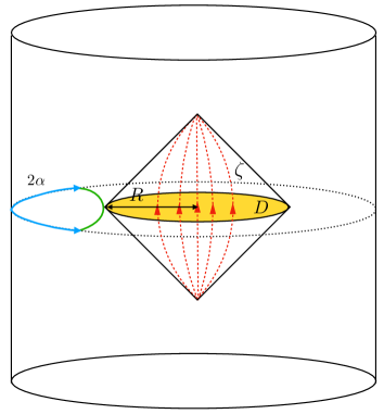
Figure 4: A causal diamond in pure AdS₃ associated to a disk $D$ (yellow region) of radius $R$. The bulk conformal Killing vector $\zeta$ generates a flow (in red) within the causal diamond, which sends the boundary of the diamond into itself, and leaves fixed the vertices and the circle $\partial D$. The minimal geodesic or Ryu-Takayanagi surface (in green), which is tangent to the circle, subtends an angle $2\alpha$ at the asymptotic boundary (in blue). Note that a larger boundary subregion corresponds to a smaller bulk disk and vice-versa.

To begin with, let us summarize the first law of causal diamonds in general relativity, derived in Jacobson:2015hqa for flat space and extended in Jacobson:2018ahi to (A)dS space. The causal diamonds under consideration are defined as the domain of dependence of (codimension-1) ball-shaped regions of any size in maximally symmetric spacetimes. There exists a unique conformal isometry that preserves these causal diamonds, which is generated by the conformal Killing vector $\zeta$. Figure 4 illustrates the flow of $\zeta$ for a causal diamond in AdS. The flow is tangent to the null boundary of the diamond, and leaves fixed the future and past vertices and the boundary of the ball. The first law applies to arbitrary first-order variations of these maximally symmetric causal diamonds to nearby solutions – i.e. the variations satisfy the linearized Einstein (constraint) equations – and it reads

$$\delta H^{\text{mat}}_{\zeta}=\frac{1}{8\pi G}\left(-\kappa\delta A+\kappa k\delta V-V_{\zeta}\delta\Lambda\right).$$ (89)

Here $\delta H^{\text{mat}}_{\zeta}$ is the variation of the bulk matter Hamiltonian which generates evolution along the flow of $\zeta$, $\kappa$ is the (positive) surface gravity associated to $\zeta$, $A$ is the area of the boundary of the ball, $k$ is the trace of the extrinsic curvature of the boundary as embedded inside the ball, $V$ is the proper volume of the ball, $V_{\zeta}$ is the thermodynamic volume defined as the proper volume locally weighted by the norm of $\zeta$, and $\Lambda$ is the cosmological constant. In the upcoming sections we compute these quantities explicitly for disks, denoted by $D$, in locally AdS₃ spacetimes.

The variations we consider in this section are of three different types, in analogy with the three CFT variations of the previous section. The first variation involves changing the boundary interval size $\alpha$ of a RT surface in a fixed global coordinate system for pure AdS. The metric of pure AdS remains the same under this variation, but the radius $R$ of the disk decreases as $\alpha$ increases (see figure 4). The second variation is a first order variation of the metric and matter fields from pure AdS to a point mass in AdS, while again keeping the coordinate system fixed. This variation is parametrized by the conical defect parameter $\epsilon$, and is related to varying the scaling dimension $\Delta$ in the dual CFT. Thirdly, we consider variations of the coupling constants of the gravitational theory, i.e. the cosmological constant $\Lambda$ and Newton’s constant $G$. Assuming the sign of the cosmological constant does not change, a variation of $\Lambda$ can also be interpreted as a metric perturbation due to changing only the curvature scale $L$ of the AdS background, since $\Lambda=-1/L^{2}$ in AdS₃. Our motivation for varying $\Lambda$ (or $L$) and $G$ is not so much that they are separate equilibrium state variables or that the quantity $-\Lambda/8\pi G$ is the pressure of a perfect fluid in the bulk Kastor:2009wy , but rather that they can be combined to form a single quantity in the dual CFT, the central charge $c=3L/(2G)$, which can be varied in the space of CFTs Kastor:2014dra . We will show that the variations of $L$ and $G$ appear in the first law in the particular combination $\delta(L/G)$, which is dual to varying the central charge of the holographic CFT. Another reason for varying $G$ is that it can be combined with the boundary area of the disk to form the differential entropy.

We start the rest of this section with a review of locally AdS₃ spacetimes with a conical defect. This enables us to compute the first-order variations of the area, volume and matter Hamiltonian for a disk in empty AdS₃. The area and volume variations match precisely with the variations of the differential entropy and holographic complexity, respectively, of the previous section. Finally, the area, volume and matter Hamiltonian variations can be combined into a single variational relation, which is the first law of causal diamonds applied to the present geometric setting.

3.1 AdS₃ with a conical defect

The AdS₃ geometry with a conical defect is locally identical to pure AdS₃ – except for one singular point – but it has a different global structure. The static geometry is constructed by cutting out a wedge of two-dimensional hyperbolic space (the spatial sections of AdS) along two spatial geodesics, and identifying the edges to form a cone. The tip of the cone is a singular point, called the ‘conical singularity’. This is a naked singularity, since it is not shielded by an event horizon. The metric takes the same form as that of pure AdS₃

$$ds^{2}=-\left(1+\frac{r^{\prime 2}}{L^{2}}\right)dt^{\prime 2}+\left(1+\frac{r^{\prime 2}}{L^{2}}\right)^{-1}dr^{\prime 2}+r^{\prime 2}d\phi^{\prime 2},$$ (90)

where $\phi$ is the bulk angular coordinate with periodicity: $\phi^{\prime}\sim\phi^{\prime}+2\pi\gamma$ where $0<\gamma<1$. The value $\gamma=1$ corresponds to vacuum AdS₃, and for $\gamma=0$ the geometry is identical to that of a massless BTZ black hole. If $\gamma=1/N$ with $N$ a positive integer, then the conical defect space corresponds to the quotient space AdS${}_{3}/\mathbb{Z}_{N}$. The conical singularity is located at $r^{\prime}=0$, and the deficit angle of the geometry is

$$\delta\phi^{\prime}=2\pi(1-\gamma)\equiv 2\pi\epsilon,$$ (91)

with $0<\epsilon<1.$ The angular periodicity can be modified by rescaling the coordinates

$$t=t^{\prime}/\gamma,\,\,\,\,\,\,\,\,\,\,r=r^{\prime}\gamma,\,\,\,\,\,\,\,\,\,\phi=\phi^{\prime}/\gamma\,.$$ (92)

Under this coordinate transformation the metric becomes

$$ds^{2}=-\left(\gamma^{2}+\frac{r^{2}}{L^{2}}\right)dt^{2}+\left(\gamma^{2}+\frac{r^{2}}{L^{2}}\right)^{-1}dr^{2}+r^{2}d\phi^{2},$$ (93)

where $\phi$ now ranges from $0$ to $2\pi$. We mainly use this coordinate system in the following sections. In appendix A we derive this metric from the embedding formalism, and we present some other metrics for conical AdS, one of which is the line element in the original paper by Deser-Jackiw Deser:1983nh (cf. equation (189)).

The conical defect geometry is not a solution to the vacuum Einstein equation, like pure AdS. It is a solution to the Einstein equation in $2+1$ dimensions with a negative cosmological constant, $G_{\mu\nu}+\Lambda g_{\mu\nu}=8\pi GT_{\mu\nu},$ and a point particle stress-energy tensor

$$\sqrt{g^{(2)}}T_{\mu\nu}u^{\mu}u^{\nu}=m\delta^{(2)}(r).$$ (94)

Obviously, the location of the classical point mass, $r=0$, coincides with the location of the conical singularity. Here we have chosen a time slice, $t=0$ for convenience, for which $g^{(2)}$ denotes the determinant of the induced metric and $u^{\mu}$ is the future directed unit normal, given by $\sqrt{g^{(2)}}=r\left(\gamma^{2}+(r/L)^{2}\right)^{-1/2}$ and $u^{\mu}\partial_{\mu}=\left(\gamma^{2}+(r/L)^{2}\right)^{-1/2}\partial_{t}$.

Next we determine the relation between the mass $m$ and the conical defect parameter $\gamma$ (see Klemm:2002ir for a similar computation). We derive the stress-energy tensor for the metric (93) from the Hamiltonian constraint

$$\mathcal{R}-2\Lambda+K^{2}-K_{\mu\nu}K^{\mu\nu}=16\pi GT_{\mu\nu}u^{\mu}u^{\nu},$$ (95)

where $\mathcal{R}$ is the intrinsic curvature scalar of the two-dimensional spacelike hypersurface. The extrinsic curvature of a constant $t$ hypersurface vanishes, i.e. $K_{\mu\nu}=0$, because the hypersurface is time symmetric. For vacuum AdS the spatial curvature scalar is thus constant: $\mathcal{R}_{\text{vac}}=2\Lambda.$ The intrinsic curvature scalar of conical AdS only differs from that of vacuum AdS at the conical singularity. Therefore, it is equal to the sum of the vacuum AdS curvature scalar and a singular part: $\mathcal{R}_{\text{con}}=2\Lambda+\mathcal{R}_{\text{sing}}.$ The singular part of the curvature scalar can be derived from the Gauss-Bonnet theorem applied to a disk of radius $R$, within the $t=0$ hypersurface and centered at $r=0$,

$$\chi_{e}=\frac{1}{4\pi}\int_{D}dV\,\mathcal{R}+\frac{1}{2\pi}\int_{\partial D}dA\,k.$$ (96)

Here $\chi_{e}$ denotes the Euler number, which is equal to one for a disk. The proper volume element of the disk is $dV=\sqrt{g^{(2)}}d\phi dr$ and the line element of the boundary circle is $dA=rd\phi$. Further, $k$ denotes the trace of the extrinsic curvature of $\partial D$ as embedded in the disk, which for the current set-up is given by

$$k=\frac{1}{\sqrt{g_{rr}}}\partial_{r}\log\sqrt{g_{\phi\phi}}\Big{|}_{r=R}=\frac{1}{R}\sqrt{\gamma^{2}+\frac{R^{2}}{L^{2}}}\,.$$ (97)

After performing some simple integrals, we obtain the relation

$$\int_{D}dV\,\mathcal{R}_{\text{sing}}=4\pi(1-\gamma).$$ (98)

Therefore, the singular part of the two-dimensional Ricci scalar is

$$\mathcal{R}_{\text{sing}}=\frac{4\pi}{\sqrt{g^{(2)}}}\left(1-\gamma\right)\delta^{(2)}(r).$$ (99)

Inserting this back into the Hamiltonian constraint (95) yields the following result for the stress-energy tensor of conical AdS₃

$$\sqrt{g^{(2)}}T_{\mu\nu}u^{\mu}u^{\nu}=\frac{1-\gamma}{4G}\delta^{(2)}({r}).$$ (100)

This is the only non-zero component of the stress-energy tensor. Comparing with (94), we find that the mass of the point particle is related to the defect parameter through

$$m=\frac{1-\gamma}{4G}=\frac{\epsilon}{4G}\,.$$ (101)

This is the expression for the mass of a point particle in flat space Deser:1983tn and in AdS Deser:1983nh . We therefore call it the Deser-Jackiw-’t Hooft (DJH) mass. It is equal to the ‘proper’ mass of the conical defect spacetime, defined as $m=\int dV\rho(r)$ where $dV$ is the ‘proper’ volume element and $\rho$ is the energy density, but it differs from the total mass of the spacetime.

We can compute the total mass of the conical defect spacetime through the ADM formula

$$M=-\frac{1}{8\pi G}\lim_{\partial D\to\infty}\int_{\partial D}dA\,N(k-k_{\gamma=1})\,.$$ (102)

Note that we have subtracted the value of the ADM mass in the pure AdS background (with $\gamma=1$) in order to cancel the divergences at spatial infinity. This is sufficient for the present context, because the first law only features the energy difference between conical AdS and pure AdS. The extrinsic trace $k$ is given by (97) and the lapse function $N$ is

$$N=\sqrt{|g_{tt}|}\Big{|}_{r=R}=\sqrt{\gamma^{2}+\frac{R^{2}}{L^{2}}}\,.$$ (103)

Inserting this into the ADM formula and taking the limit $R\to\infty$ yields

$$M=\frac{1-\gamma^{2}}{8G}=\frac{\epsilon}{4G}-\frac{\epsilon^{2}}{8G}\,.$$ (104)

Note that for small deficit angles, i.e. $\epsilon\ll 1$, the ADM mass agrees with the DJH mass. This implies that we can use both masses interchangeably in the first law of causal diamonds, since the first law only holds for first order perturbations away from pure AdS. For large deficit angles, however, the ADM mass contains an extra $O(\epsilon^{2})$ term compared to the DJH mass. This term could be related to the binding energy of the point mass to the gravitational background. The (negative) gravitational binding energy is defined as the difference between the total mass and the proper mass

$$E_{B}=M-m=-\frac{\epsilon^{2}}{8G}\,.$$ (105)

The negative binding energy might be interpreted as a reduction in the gravitational energy due to the fact that the conical defect cuts out part of the spacetime Balasubramanian:2001nb . Because we are interested only in small point masses, we neglect this binding energy in the remainder of the paper.

Finally, we would like to mention a simple relation between the DJH and ADM mass

$$m=\frac{1}{4G}\left(1-\sqrt{1-8GM}\right),$$ (106)

and we remark that the ADM mass (not the DJH mass) is related to the scaling dimension in the $2d$ CFT, via $\Delta=ML.$ This can be seen, for example, by comparing the ADM mass (104) and the conformal dimension of a twist operator (35), where one should restrict to integer values for the conical defect parameter, i.e. $1/\gamma=N\in\mathbb{N}$ (see footnote 12).

3.2 First law of causal diamonds in AdS₃

3.2.1 Area variation

In this section we compute the variation of the boundary area of a circular disk, centered at the point $r=0$ in a constant time slice of pure AdS₃. In order to compare the area variation with the differential entropy variation in the CFT, we express the radius $R$ of the disk in terms of the boundary opening angle $\alpha$. By construction, the spacelike geodesic anchored at the endpoints of the boundary interval of size $2\alpha$ is tangent to the boundary circle of the disk (see figure 4). If the AdS spacetime contains a conical singularity, the coordinate radius of the disk is given by

$$R=L\gamma\cot(\gamma{\alpha})\,.$$ (107)

The area of the disk in conical AdS₃ is therefore

$$A_{\text{con}}=2\pi R=2\pi L\left[\frac{\cos\alpha}{\sin\alpha}+\left(-\frac{\cos\alpha}{\sin\alpha}+\frac{\alpha}{\sin^{2}\alpha}\right)\epsilon+\mathcal{O}\left(\epsilon^{2}\right)\right].$$ (108)

We see that the area in conical AdS depends on three variables, $A_{\text{con}}=A_{\text{con}}(\alpha,\epsilon,L)$. The area in pure AdS depends only on two variables, $A_{\text{vac}}=A_{\text{vac}}(\alpha,L)$, since the defect parameter is fixed to be $\epsilon_{\text{vac}}=0.$ We therefore consider three types of first-order variations of the pure AdS background: 1) variations of $\alpha$, i.e. rescaling the size of the boundary interval, 2) variations of $\epsilon$, i.e. metric perturbations due to the presence of a conical singularity in AdS₃, and 3) variations of $L$, i.e. changing the cosmological constant of the background (in the differential entropy variation below we also include variations of the gravitational constant). The total change in area under $\alpha$, $\epsilon$ and $L$ variations is defined as

$$\delta A=\delta_{\alpha}A\Big{|}_{\epsilon,L}+\delta_{\epsilon}A\Big{|}_{\alpha,L}+\delta_{L}A\Big{|}_{\alpha,\epsilon}.$$ (109)

First, the change in area under an $\alpha$ variation, at fixed $\epsilon$ and $L$, is to first order

$$\delta_{\alpha}A\Big{|}_{\epsilon,L}=\frac{\partial A_{\text{vac}}}{\partial\alpha}\delta\alpha=-2\pi L\frac{1}{\sin^{2}\alpha}\delta\alpha.$$ (110)

Here we used an explicit expression for the area in pure AdS,

$$A_{\text{vac}}=2\pi L\cot\alpha,$$ (111)

which follows from (108) by setting $\epsilon=0$. Thus, the area decreases if the boundary interval becomes larger. This can be easily verified from figure 4.

Further, from (108) we see that the area change due to an infinitesimal variation of the conical defect parameter is, keeping $\alpha$ and $L$ fixed,

$$\delta_{\epsilon}A\Big{|}_{\alpha,L}=2\pi L\left(-\frac{\cos\alpha}{\sin\alpha}+\frac{\alpha}{\sin^{2}\alpha}\right)\delta\epsilon,$$ (112)

where we introduced $\delta\epsilon=\epsilon_{\text{con}}-\epsilon_{\text{vac}}=\epsilon$, since $\epsilon_{\text{vac}}=0$. The function of $\alpha$ between brackets is positive since $\alpha\geq 0$, and we have $\delta\epsilon>0$ since the perturbed geometry has a conical defect. Therefore, the area of the disk increases due to the presence of a conical defect, if the background curvature and boundary opening angle are kept fixed.

Finally, if we vary the AdS radius, but keep $\alpha$ and $\epsilon$ fixed, the area change is simply

$$\delta_{L}A\Big{|}_{\alpha,\epsilon}=\frac{\partial A_{\text{vac}}}{\partial L}\delta L=2\pi\frac{\cos\alpha}{\sin\alpha}\delta L.$$ (113)

Thus, the full area variation is to first order given by

$$\delta A=2\pi\frac{\cos\alpha}{\sin\alpha}\delta L-2\pi L\frac{1}{\sin^{2}\alpha}\delta\alpha+2\pi L\left(-\frac{\cos\alpha}{\sin\alpha}+\frac{\alpha}{\sin^{2}\alpha}\right)\delta\epsilon.$$ (114)

In order to compare the area variation of a disk in pure AdS₃ with the variation of the differential entropy, we need the holographic dictionary between differential entropy and bulk area Balasubramanian:2013rqa ; Balasubramanian:2013lsa

$$S_{\text{diff}}=\frac{A}{4G}.$$ (115)

If we allow for variations of Newton’s constant $G$, the variation of the differential entropy is, written in terms of bulk quantities,

$$\delta S_{\text{diff}}=\frac{\pi}{2}\frac{\cos\alpha}{\sin\alpha}\delta\left(\frac{L}{G}\right)-\frac{\pi L}{2G}\frac{1}{\sin^{2}\alpha}\delta\alpha+\frac{\pi L}{2G}\left(-\frac{\cos\alpha}{\sin\alpha}+\frac{\alpha}{\sin^{2}\alpha}\right)\delta\epsilon.$$ (116)

Note that the variation of the ratio of the AdS radius and Newton’s constant appears in this formula, since the (vacuum) differential entropy is proportional to the same fraction: $S_{\text{vac}}^{\text{DE}}\sim L/G$. We can now translate the right-hand side of the equation above in terms of pure boundary quantities, using the standard holographic dictionary for AdS₃/CFT₂

$$c=\frac{3L}{2G}\qquad\text{and}\qquad\Delta=ML=\frac{c}{12}\left(1-\gamma^{2}\right)=\frac{c}{6}\epsilon+\mathcal{O}(\epsilon^{2}).$$ (117)

The first equation is the Brown-Henneaux formula for the central charge Brown:1986nw , and the second equation is the holographic relation between the scaling dimension of an operator in the dual CFT and the ADM mass of the (conical) geometry. Importantly, the first term on the right-hand side of (116) can be written solely in terms of the variation of the central charge, due to the appearance of $\delta(L/G)$. Furthermore, the final term in (116) is proportional to the variation of the scaling dimension, since $\delta\Delta=(c/6)\delta\epsilon$ (36). Therefore, based on the holographic dictionary we arrive at

$$\delta S_{\text{diff}} =\frac{\pi}{3}\frac{\cos\alpha}{\sin\alpha}\delta c-\frac{\pi c}{3}\frac{1}{\sin^{2}\alpha}\delta\alpha+2\pi\left(-\frac{\cos\alpha}{\sin\alpha}+\frac{\alpha}{\sin^{2}\alpha}\right)\delta\Delta.$$ (118)

This is identical to the differential entropy variation derived in section 2.2.1.

3.2.2 Volume variation

In this section we vary the proper volume of a disk in pure AdS₃. We consider again the three ($\alpha,\epsilon,L$) variations of the previous section, under which the volume changes to first order as

$$\delta V=\delta_{\alpha}V\Big{|}_{\epsilon,L}+\delta_{\epsilon}V\Big{|}_{\alpha,L}+\delta_{L}V\Big{|}_{\alpha,\epsilon}.$$ (119)

The $\alpha$ and $L$ variations can be derived from the proper volume in pure AdS

$$V_{\text{vac}}=\int_{0}^{R}\frac{2\pi rdr}{\sqrt{1+(r/L)^{2}}}=2\pi L^{2}\left(\sqrt{1+(R/L)^{2}}-1\right)=2\pi L^{2}\left(\frac{1}{\sin\alpha}-1\right).$$ (120)

The change of volume under a variation of $\alpha$, at fixed $\epsilon$ and $L$, is given by

$$\delta_{\alpha}V\Big{|}_{\epsilon,L}=\frac{\partial V_{\text{vac}}}{\partial\alpha}\delta\alpha=-2\pi L^{2}\frac{\cos\alpha}{\sin^{2}\alpha}\delta\alpha.$$ (121)

The minus sign indicates that in pure AdS the volume of a disk decreases if the opening angle on the boundary increases (and $L$ is kept fixed). Further, because of the quadratic scaling of the volume with the AdS radius, the change in volume under a variation of $L$, at fixed $\alpha$ and $\epsilon$, is

$$\delta_{L}V\Big{|}_{\alpha,\epsilon}=\frac{\partial V_{\text{vac}}}{\partial L}\delta L=4\pi L\left(\frac{1}{\sin\alpha}-1\right)\delta L.$$ (122)

We simply find that in pure AdS the volume of a disk increases if the curvature radius increases (and $\alpha$ is kept fixed).

The $\epsilon$ variation in (119) is equal to the first order change in the volume due to the presence of a conical defect in AdS. In order to derive this we need the proper volume of a disk in AdS with a conical defect, which in terms of the coordinates (93) is given by

$$V_{\text{con}}=\int_{0}^{R}\frac{2\pi rdr}{\sqrt{\gamma^{2}+r^{2}/L^{2}}}=2\pi L^{2}\left(\sqrt{\gamma^{2}+R^{2}/L^{2}}-\gamma\right).$$ (123)

Although we use the same notation $R$ in conical AdS and in pure AdS for the coordinate radius of a disk, we emphasize that its relation to, for instance, the geodesic radius of the disk or to the boundary opening angle $\alpha$, as in (107), is different for conical and pure AdS, since their metrics differ. In terms of the boundary opening angle, the proper volume reads

$$V_{\text{con}} =2\pi L^{2}\gamma\left(\frac{1}{\sin(\alpha\gamma)}-1\right)$$ (124)

$$=2\pi L^{2}\left[\frac{1}{\sin\alpha}-1+\left(\frac{\alpha\cos\alpha}{\sin^{2}\alpha}-\frac{1}{\sin\alpha}+1\right)\epsilon+\mathcal{O}\left(\epsilon^{2}\right)\right].$$

In the last equation we expanded the proper volume around $\epsilon_{\text{vac}}=0.$ The leading-order term in the expansion is, of course, the proper volume in pure AdS. The subleading-order term defines the first order volume change under a variation of $\epsilon$, at fixed $\alpha$ and $L$,

$$\delta_{\epsilon}V\Big{|}_{\alpha,L} =2\pi L^{2}\left(\frac{\alpha\cos\alpha}{\sin^{2}\alpha}-\frac{1}{\sin\alpha}+1\right)\delta\epsilon.$$ (125)

The term between brackets is positive for the entire range of $\alpha$, i.e. for $0\leq\alpha\leq\pi/2$. Hence, just like the area, the proper volume of a disk increases due to the presence of a point particle in AdS, if $\alpha$ and $L$ are kept fixed. In total, the volume variation is given by

$$\delta V=4\pi L\left(\frac{1}{\sin\alpha}-1\right)\delta L-2\pi L^{2}\frac{\cos\alpha}{\sin^{2}\alpha}\delta\alpha+2\pi L^{2}\left(\frac{\alpha\cos\alpha}{\sin^{2}\alpha}-\frac{1}{\sin\alpha}+1\right)\delta\epsilon.$$ (126)

Next, we want to convert this bulk variational identity for the volume into a boundary variational identity for holographic complexity. We employ the ‘complexity=volume’ conjecture Susskind:2014rva ; Stanford:2014jda , which can be extended to a correspondence between the complexity of the vacuum state in a cutoff CFT and the volume of a ball-shaped region in the bulk, whose radius is related to the dual energy cutoff scale in the CFT (see section 2.1.3)

$$\mathcal{C}=\frac{V}{4GL}\,.$$ (127)

Allowing for variations of both Newton’s constant and the AdS radius, we thus find the following variational relation for holographic complexity in terms of bulk quantities

$$\delta\mathcal{C}=\frac{\pi}{2}\left(\frac{1}{\sin\alpha}-1\right)\delta\left(\frac{L}{G}\right)-\frac{\pi L}{2G}\frac{\cos\alpha}{\sin^{2}\alpha}\delta\alpha+\frac{\pi L}{2G}\left(\frac{\alpha\cos\alpha}{\sin^{2}\alpha}-\frac{1}{\sin\alpha}+1\right)\delta\epsilon.$$ (128)

The variation $\delta(L/G)$ appears again, just like in the differential entropy variation (116), because the vacuum holographic complexity scales with the same fraction: $\mathcal{C}_{\text{vac}}\sim L/G$. This term is proportional to the variation of the central charge (117). Note that with a different normalization of holographic complexity, such as topological complexity $\mathcal{C}_{\text{top}}=V/L^{2}$ Abt:2017pmf ; Abt:2018ywl , the complexity variation would not involve a term proportional to the variation of the central charge, since $C_{\text{top}}^{\text{vac}}$ does not depend on the central charge, cf. equation (33). With our choice of normalization, however, the complexity variation can be written in terms of the variation of the three CFT variables ($c,\alpha,\Delta$), by employing the holographic dictionary for AdS₃/CFT₂,

$$\delta\mathcal{C}=\frac{\pi}{3}\left(\frac{1}{\sin\alpha}-1\right)\delta c-\frac{\pi c}{3}\frac{\cos\alpha}{\sin^{2}\alpha}\delta\alpha+2\pi\left(\frac{\alpha\cos\alpha}{\sin^{2}\alpha}-\frac{1}{\sin\alpha}+1\right)\delta\Delta.$$ (129)

As expected, this agrees with the result derived in section 2.2.2.

3.2.3 Bulk matter Hamiltonian variation

In this section we compute the variation of the bulk matter Hamiltonian, $\delta H_{\zeta}^{\text{mat}}$, featuring on the left-hand side of the first law of causal diamonds (89). The matter Hamiltonian is the generator of evolution of matter fields along the flow generated by the conformal Killing vector $\zeta$. Its first-order variation takes the form Jacobson:2018ahi

$$\delta H_{\zeta}^{\text{mat}}=\int_{D}\delta({T_{\mu}}^{\nu})\zeta^{\mu}u_{\nu}dV.$$ (130)

Recall that $u$ is the future pointing unit normal to the disk $D$. Moreover, ${T_{\mu}}^{\nu}=g^{\nu\alpha}T_{\mu\alpha}$ denotes the Hilbert stress-energy tensor (with one index raised) associated to matter fields in the bulk. Since the stress-energy tensor for a typical field theory action is quadratic in the matter fields, and the matter fields vanish in the AdS background, the first-order variation of the stress tensor away from pure AdS vanishes. The stress-energy associated to fluid matter, however, can contribute to the first-order variation of the Hamiltonian, and thus to the first law of causal diamonds.

For the present field content, the perfect fluid consists of a point mass in AdS and its stress-energy indeed contributes to the matter Hamiltonian variation. Inserting the point particle stress-energy tensor (94) into the matter Hamiltonian variation (130) yields

$$\delta H_{\zeta}^{\text{mat}}=\int_{D}d\phi dr\delta^{(2)}(r)(-\zeta\cdot u)\delta m=\sqrt{-\zeta\cdot\zeta}\Big{|}_{O}\delta m,$$ (131)

where $\delta m$ is the variation of the DJH mass and $O$ is the location of the point particle, i.e. $O=\{t=0,r=0\}$ for the current set-up. In the first equality we used that $u$ has unit norm, $u\cdot u=-1$, and in the last equality we wrote $u$ as the velocity vector of the conformal Killing flow, $u^{\mu}=\zeta^{\mu}/\sqrt{-\zeta\cdot\zeta}$, which also defines the extension of $u$ off of $D$. This relation between $u$ and $\zeta$ holds in particular at $D$ because the conformal Killing vector is normal to the disk. We thus find that the Hamiltonian generating the evolution of a point mass along the conformal Killing flow is equal to the DJH mass times a ‘redshift factor’

$$H_{\zeta}^{\text{mat}}=m\sqrt{-\zeta\cdot\zeta}\Big{|}_{O}=m\frac{\partial\tau}{\partial s}\Big{|}_{O}.$$ (132)

This result was to be expected, since $H_{\zeta}^{\text{mat}}$ and $m$ are defined with respect to different time variables, called $s$ and $\tau$ respectively. The conformal Killing time $s$ satisfies $\zeta\cdot ds=1$, with the initial condition $s=0$ at $D$, and the time variable $\tau$ is the proper time along the flow lines of $\zeta$, which is similarly defined through $u\cdot d\tau=1$ and the condition $\tau=0$ at $D$. However, the function $s$ is not uniquely defined, and is only meaningful relative to a complete coordinate system. In appendix B of Jacobson:2018ahi a complete coordinate chart $(x,s)$ was constructed for a maximally symmetric diamond (suppressing the angular coordinates). Here $x\in[0,\infty)$ is a radial coordinate, satisfying $|dx|=|ds|$, $x=0$ at $r=0$, and $\zeta\cdot dx=0$. This implies in particular that $\zeta=\partial_{s}$ and $\tau=\tau(s,x).$ Thus from the definitions of $\tau$ and $u$ we find $\zeta\cdot d\tau=\sqrt{-\zeta\cdot\zeta}$, which is identical to the second equality in (132) since $\zeta\cdot d\tau=\partial\tau/\partial s$.

The unique conformal Killing vector whose flow preserves a spherically symmetric causal diamond in AdS reads in terms of the standard $t$ and $r$ coordinates Jacobson:2018ahi

$$\zeta=-\frac{2\pi L^{2}}{R}\left[\left(1-\frac{\sqrt{1+(R/L)^{2}}}{\sqrt{1+(r/L)^{2}}}\cos(t/L)\right)\partial_{t}+\frac{R}{L}\sqrt{(1+(R/L)^{2})(1+(r/L)^{2})}\sin(t/L)\partial_{r}\right].$$ (135)

The vector $\zeta$ generates a timelike flow within the causal diamond, it acts as a null flow on the null boundaries and it vanishes at the edge of the diamond and the future and past tips. We normalized the conformal Killing vector such that its surface gravity is $\kappa=2\pi$, in contrast to Jacobson:2018ahi where the normalization of $\zeta$ was chosen such that $\kappa=1$. The definition of surface gravity used in this setup is: $\nabla_{\mu}(\zeta\cdot\zeta)=-2\kappa\zeta_{\mu}$, where both sides are evaluated on the (future) null boundary of the diamond, which is a conformal Killing horizon since $\zeta$ is tangent to its null generators. This definition of surface gravity is Weyl invariant Jacobson:1993pf and constant on any bifurcate conformal Killing horizon (see appendix C of Jacobson:2018ahi ). The value $\kappa=2\pi$ is convenient, since the Hawking temperature $T_{\text{H}}=\kappa/2\pi$ is equal to one for this normalization. Therefore, the conjugate quantities to the differential entropy and holographic complexity simplify considerably in the CFT first law, cf. (77).

The norm of the conformal Killing vector evaluated at the center of the diamond is

$$\sqrt{-\zeta\cdot\zeta}\Big{|}_{O} =\frac{2\pi L^{2}}{R}\left(\sqrt{1+(R/L)^{2}}-1\right)=2\pi Lf(\alpha)$$ (136)

$$\text{with}\quad f(\alpha) =\left(\frac{1}{\cos\alpha}-\frac{\sin\alpha}{\cos\alpha}\right),$$

where the factor $2\pi$ arises due to our choice of $\kappa$. The variation of the point particle Hamiltonian now follows from inserting this norm and the variation of the DJH mass, $\delta m=\delta\epsilon/(4G)$, into equation (131)

$$\delta H_{\zeta}^{{\text{mat}}}=\frac{\pi L}{2G}f(\alpha)\delta\epsilon.$$ (137)

Note that the gravitational constant is not being varied in this variational expression, since $\epsilon$ vanishes in the background spacetime. The change in the matter Hamiltonian is, of course, positive since the norm of $\zeta$ is positive and $\delta\epsilon>0$ by assumption. Using the holographic dictionary (117) the Hamiltonian variation can be easily expressed purely in terms of CFT quantities

$$\delta H_{\zeta}^{\text{mat}}=2\pi f(\alpha)\delta\Delta.$$ (138)

We recognize here the CFT energy variation, defined in (74), in the first law for differential entropy. The matter Hamiltonian itself (132) is given by

$$H^{\text{mat}}_{\zeta}=2\pi f(\alpha)mL=2\pi f(\alpha)(c/6)\epsilon,$$ (139)

which reads in terms of the conformal dimension of the twist operator

$$H^{\text{mat}}_{\zeta}=2\pi f(\alpha)(c/6)(1-\sqrt{1-12\Delta/c}).$$ (140)

Therefore, the boundary energy $E$ dual to the matter Hamiltonian is equal to this expression up to all orders in $\Delta/c$ (or $\epsilon$). Up to first order in $\Delta/c$ it is equal to $2\pi f(\alpha)\Delta$, which is the only term that is relevant for the first law studied in this paper. Note that since $\Delta=ML$, the difference between the leading order term and the full expression for the matter Hamiltonian precisely corresponds to the difference between the ADM mass $M$ and the DJH mass $m$, respectively. In other words, the expression (140) for $H^{\text{mat}}_{\zeta}$ above also follows from inserting the relation (106) between the DJH and the ADM mass into (139).

3.2.4 Combining the variations

In the previous three sections we computed the area variation, volume variation and matter Hamiltonian variation for disks in three-dimensional AdS space. In this section we combine these three variations into one variational relation, thereby reproducing the first law of causal diamonds applied to variations from pure AdS to conical AdS space.

We proceed by studying the following combination of variations for the present set-up, which appears in the first law of causal diamonds (89),

$$\delta A-k\delta V,\qquad\text{with}\qquad k=\frac{1}{R}\sqrt{1+(R/L)^{2}}=\frac{1}{L\cos\alpha}$$ (141)

being the trace of the outward extrinsic curvature of $\partial D$ as embedded in the disk $D$. Below we compute this combination explicitly for the $\alpha,\epsilon$ and $L$ variations. That is, we define the area and volume change by equations (109) and (119), respectively, and insert the results of the previous sections for the ($\alpha,\epsilon,L$) variations.

Firstly, it follows from (110) and (121) that the combination of variations above for variations which alter $\alpha$, but keep $\epsilon$ and $L$ fixed, vanishes

$$\left(\delta_{\alpha}A-k\delta_{\alpha}V\right)\Big{|}_{\epsilon,L}=0.$$ (142)

This is because, by definition, the trace of the extrinsic curvature is equal to $k=(\partial A/\partial V)_{L}.$ If the boundary opening angle varies, the volume change is given by $\delta_{\alpha}V\big{|}_{\epsilon,L}=(\partial_{\alpha}V)_{L}\delta\alpha$, while the area change is $\delta_{\alpha}A\big{|}_{\epsilon,L}=(\partial_{\alpha}A)_{L}\delta\alpha=k(\partial_{\alpha}V)_{L}\delta\alpha$, hence equation (142) follows. A more formal reason is that the variation induced by rescaling $\alpha$ is a diffeomorphism, and it was shown in section 3.3.2 of Jacobson:2018ahi that the combination (141) vanishes for any diffeo-induced variation. Below we can thus leave out the restriction of fixing $\alpha$ in the combination of variations under consideration.

Secondly, for first-order variations of $\epsilon$, at fixed $L$, the combination of area and volume variations becomes

$$\left(\delta_{\epsilon}A-k\delta_{\epsilon}V\right)\Big{|}_{L}=-2\pi L\left(\frac{1}{\cos\alpha}-\frac{\sin\alpha}{\cos\alpha}\right)\delta\epsilon.$$ (143)

Here we inserted expressions (112) and (125), respectively, for the area and volume variation induced by $\epsilon$. The right-hand side is related to minus the matter Hamiltonian variation (137), hence we find the following relation for $\epsilon$ induced variations

$$\frac{1}{4G}\left(\delta_{\epsilon}A-k\delta_{\epsilon}V\right)\Big{|}_{L}=-\delta H_{\zeta}^{\text{mat}}.$$ (144)

The minus sign indicates that the area at fixed volume decreases due to the presence of a conical defect, while the volume increases at fixed area.

Thirdly, for variations which change the AdS radius, at fixed $\epsilon$, the combination of variations takes the form

$$\left(\delta_{L}A-k\delta_{L}V\right)\Big{|}_{\epsilon}=-2\pi\left(\frac{2}{\cos\alpha\sin\alpha}-\frac{2}{\cos\alpha}-\frac{\cos\alpha}{\sin\alpha}\right)\delta L.$$ (145)

This follows from expressions (113) and (122), respectively, for the area and volume change under a variation of $L$. The variation of the AdS radius is related to the variation of the cosmological constant, via $-2\delta L/L=\delta\Lambda/\Lambda$. The conjugate quantity to $\delta L$ is therefore proportional to the so-called ‘thermodynamic volume’ $V_{\zeta}$, which appears in extensions of the first law of black hole mechanics as the quantity conjugate to $\delta\Lambda$ Kastor:2009wy ; Dolan:2010ha ; Cvetic:2010jb . The thermodynamic volume of maximally symmetric causal diamonds is defined as the proper volume weighted by the norm of $\zeta$ Jacobson:2018ahi

$$V_{\zeta}=\int_{D}dV\sqrt{-\zeta\cdot\zeta}\,.$$ (146)

It can be computed explicitly for the conformal Killing vector (135) of a causal diamond in pure AdS

$$V_{\zeta} =\frac{2\pi L^{2}}{R}\left(\pi R^{2}-2\pi L^{2}\left(\sqrt{1+(R/L)^{2}}-1\right)\right)$$ (147)

$$=2\pi^{2}L^{3}\left(\frac{\sin\alpha}{\cos\alpha}+\frac{1}{\cos\alpha\sin\alpha}-\frac{2}{\cos\alpha}\right).$$

Since the (positive) functions of $\alpha$ within parenthesis in equations (145) and (147) are the same, we can rewrite the former relation as

$$\left(\delta_{L}A-k\delta_{L}V\right)\Big{|}_{\epsilon}=-\frac{V_{\zeta}}{2\pi}\frac{2}{L^{3}}\delta L=-\frac{V_{\zeta}}{2\pi}\delta\Lambda.$$ (148)

From this variational identity and the scaling properties $A\sim L$ and $V\sim L^{2}$ one can easily obtain a Smarr-like relation between the area, volume, cosmological constant and their conjugate quantities

$$A-2kV=\frac{V_{\zeta}}{2\pi}2\Lambda.$$ (149)

This is indeed the Smarr formula in three spacetime dimensions for maximally symmetric causal diamonds with $\kappa=2\pi$, derived in Jacobson:2018ahi .

Finally, by combining the $\alpha$, $L$ and $\epsilon$ variations (142), (144) and (148), respectively, we arrive at the variational identity which relates the variations of the area, volume, matter Hamiltonian and cosmological constant

$$\frac{1}{4G}\left(\delta A-k\delta V\right)=-\delta H_{\zeta}^{\text{mat}}-\frac{V_{\zeta}}{8\pi G}\delta\Lambda.$$ (150)

This agrees with the first law of causal diamonds (89) if we make the identification $\kappa=2\pi$.

Note that in the first law of causal diamonds only the variation of the cosmological constant of the Lagrangian theory appears, and not of Newton’s constant. The absence of the variation of Newton’s constant in (150) is crucial for the comparison of the gravitational bulk first law with the microscopic boundary first law (see section 4.1 below). Ultimately, the reason for this absence is that the area, volume and matter Hamiltonian do not depend on the gravitational constant, whereas the first two quantities do scale with the cosmological constant. For completeness, in appendix D we provide a careful analysis of the variations of the coupling constants in the covariant phase space formalism, and we prove that the terms proportional to the variation of $G$ cancel out in the first law of causal diamonds. For variation of $\Lambda$ such an analysis was done in Jacobson:2018ahi by treating the cosmological constant as a perfect fluid, and thus as part of the fluid stress-energy tensor. However, variations of $G$ cannot be computed in this way and hence an independent analysis is needed.

As the gravitational constant is a coupling constant of the Lagrangian theory, it could in principle be varied in the space of gravitational theories (see Kastor:2010gq ; Kastor:2014dra ; Caceres:2016xjz ; Kastor:2016bph for other references where variations of all gravitational constants are taken into account in extended first laws). For example, in contrast to the extended first law of causal diamonds, in the extended version of the first law for AdS-Schwarzschild black holes the variations of $\Lambda$ and $G$ could both contribute

$$\delta M=\frac{1}{8\pi G}\left(\kappa\delta A+\bar{V}_{\chi}\delta\Lambda\right)-M\,\frac{\delta G}{G}.$$ (151)

Here $\bar{V}_{\chi}$ is the background subtracted thermodynamic volume (denoted by $\Theta$ in Kastor:2009wy ), and $\chi$ represents the timelike Killing field of AdS-Schwarzschild. The variations $\delta\Lambda$ and $\delta G$ could both appear in the first law, because the mass $M$ depends on $\Lambda$ and $G$ via the Smarr formula, which is given by Kastor:2009wy

$$\frac{d-3}{d-2}M=\frac{1}{8\pi G}\left(\kappa A-\frac{2}{d-2}\bar{V}_{\chi}\Lambda\right)$$ (152)

in $d$ spacetime dimensions. The $\delta G$ term in the first law (151), which is perhaps unfamiliar to the reader, arises simply due to the scaling $M\sim G^{-1}$ in the Smarr formula. Although we take the variations of the couplings $\Lambda$ and $G$ into account in the first law, in this paper we do not view them as thermodynamic variables in the bulk; rather the number of degrees of freedom $N_{\text{dof}}\sim L^{d-2}/G$ plays the role of a thermodynamic variable in a holographic CFT. The variations of $\Lambda$ and $G$ in the first law of AdS black holes correspond to a chemical potential term for varying the number of degrees of freedom in the dual CFT first law (i.e. $\mu\delta N_{\text{dof}}$ term with $\mu$ the chemical potential), but only if the CFT first law is expressed in terms of the dimensionless energy $E=ML$ Visser . In the next section, we investigate how such a $\mu\delta N_{\text{dof}}$ term arises in the CFT dual of the first law of causal diamonds.

4 Matching the boundary and bulk first laws

In section 2 we derived a new variational relation in two-dimensional CFTs for differential entropy and holographic complexity, and in section 3 we analyzed the first law of causal diamonds for metric perturbations from vacuum AdS₃ to the conical defect geometry. In the present section we show that the boundary first law of section 2 is the holographic dual of the bulk first law of section 3. In section 4.1 we derive the boundary first law from the bulk first law, using the holographic dictionary in AdS₃/CFT₂. In section 4.2 we generalize this argument to arbitrary dimensions – assuming the dictionary between differential entropy and the bulk area generalizes to higher dimensions – thereby obtaining a new variational identity for higher-dimensional holographic CFTs.

4.1 First law in holographic CFT₂ from first law in AdS₃

We want to express the first law of causal diamonds in terms of variations of the differential entropy and holographic complexity, for which we repeat here the holographic dictionary used in this paper

$$S_{\text{diff}}=\frac{A}{4G}\qquad\text{and}\qquad\mathcal{C}=\frac{V}{4GL}.$$ (153)

Since we allow for variations of Newton’s constant $G$ and the AdS radius $L$, the variations of the differential entropy and complexity are not proportional to the variations of the area and proper volume, respectively, which appear in the first law of causal diamonds. For example, the inclusion of a factor $1/G$ inside the variation of the area has to be compensated by a term involving the variation of Newton’s constant, i.e. $(\delta A)/G=\delta(A/G)-A\delta(1/G)$. Therefore, the area and volume variations are, respectively, related to the variations of differential entropy and holographic complexity via

$$\frac{1}{4G}\delta A =\delta\left(\frac{A}{4G}\right)+\frac{A}{4G}\frac{\delta G}{G},$$ (154)

$$\frac{1}{4G}\delta V =L\,\delta\!\left(\frac{V}{4GL}\right)+\frac{V}{4G}\frac{\delta G}{G}+\frac{V}{4G}\frac{\delta L}{L}.$$ (155)

If we insert these relations into the first law, we find a variational relation which now does involve a term proportional to $\delta G$, in addition to a new term proportional to $\delta L$. The term involving $\delta L$ in (155) can be combined with the $\delta\Lambda$ term in the first law, by using the relation $-2\delta L/L=\delta\Lambda/\Lambda$ and the Smarr formula (149). We thus obtain a new form of the first law of causal diamonds (150), in which the variations $\delta L$ and $\delta G$ share a common prefactor and appear in a particular combination,

$$\delta\!\left(\frac{A}{4G}\right)-kL\,\delta\!\left(\frac{V}{4GL}\right)=\left(\frac{A}{4G}-kL\frac{V}{4GL}\right)\left(\frac{\delta L}{L}-\frac{\delta G}{G}\right)-\delta H_{\zeta}^{\text{mat}}.$$ (156)

This form of the first law can be easily translated into a boundary first law by using the holographic dictionary of the AdS₃/CFT₂ correspondence. On the left-hand side we find the variations of the differential entropy and holographic complexity (153). The conjugate quantity $kL$ to the variation of the complexity is a dimensionless function of the boundary opening angle, i.e. $1/\cos\alpha$, since $k$ is given by (141). On the right-hand side, the combination of variations $\delta L/L-\delta G/G$ is equal to $\delta(L/G)/(L/G)$ and hence to $\delta c/c$, where $c$ is the central charge of a dual $2d$ CFT. The boundary first law which follows from the bulk first law is therefore

$$\delta S_{\text{diff}}-\frac{1}{\cos\alpha}\delta\mathcal{C}=\left(S_{\text{diff}}-\frac{1}{\cos\alpha}\mathcal{C}\right)\frac{\delta c}{c}-2\pi\left(\frac{1}{\cos\alpha}-\frac{\sin\alpha}{\cos\alpha}\right)\delta\Delta,$$ (157)

where we also replaced the matter Hamiltonian variation by expression (138) involving the variation of the scaling dimension. This result agrees, of course, with the boundary first law derived in section 2.2.3. The reason behind the appearance of $\delta L/L-\delta G/G$ (or $\delta c/c$) in the first law is that both differential entropy and our definition of holographic complexity are proportional to the fraction $L/G$ (or $c$). The fact that differential entropy and complexity are proportional to a (generalized) central charge in the CFT, and hence that the variations of $L$ and $G$ in the first law combine into the variation of the central charge, generalizes to higher dimensions, as we will see in the next section.

Before moving on, we stress that the validity of the CFT dual of the first law of causal diamonds depends on the holographic dictionary for the area and volume variation. Since the dictionary for holographic complexity has not been established yet, it could be that $\mathcal{C}=V/(4GL)$ is incorrect. As an example of a different expression, we consider topological complexity (32), $\mathcal{C}_{\text{top}}:=-\frac{1}{2}\int_{D}dV\mathcal{R}=V/L^{2}$, which is motivated from the Gauss-Bonnet theorem (96) Abt:2017pmf . We note that in this case the first law of causal diamonds can be organized as

$$\delta\!\left(\frac{A}{4G}\right)-\frac{kL}{6}\frac{3L}{2G}\delta\left(\frac{V}{L^{2}}\right)=\frac{A}{4G}\left(\frac{\delta L}{L}-\frac{\delta G}{G}\right)-\delta H_{\zeta}^{\text{mat}}.$$ (158)

This suggests a CFT first law for differential entropy and topological complexity of the form

$$\delta S_{\text{diff}}-\frac{c}{6\cos\alpha}\delta\mathcal{C}_{\text{top}}=S_{\text{diff}}\frac{\delta c}{c}-2\pi\left(\frac{1}{\cos\alpha}-\frac{\sin\alpha}{\cos\alpha}\right)\delta\Delta.$$ (159)

The conjugate quantities to the complexity variation and to the central charge variation are then slightly different compared to the CFT first law (157). This signifies how important it is to establish the correct dictionary for the volume. In higher dimensions, however, the dictionary for holographic complexity used in this paper seems to be more appropriate than topological complexity, since the latter is not a dimensionless quantity for spacetime dimensions $d>3$ (because $V\sim L^{d-1}$ and $\mathcal{R}=2\Lambda\sim 1/L^{2}$ for static slices of pure AdS).

4.2 Extension of the boundary first law to higher dimensions

The bulk first law in the form (150) applies to causal diamonds in AdS space in arbitrary dimensions Jacobson:2018ahi . Following the same procedure as in the previous section, we can thus derive a boundary first law in higher dimensions from the bulk first law. This translation procedure, however, is highly dependent on the holographic dictionary (153) for differential entropy and complexity, and the question is whether this dictionary generalizes to higher dimensions. Since the original ‘complexity=volume’ conjecture Susskind:2014rva ; Stanford:2014jda is not restricted to any specific dimension, we can safely assume the dictionary between holographic complexity (for cutoff CFTs) and proper volume in higher dimensions.

Furthermore, differential entropy has been extended to higher dimensions for certain symmetric gravitational backgrounds by Myers:2014jia ; Czech:2014wka and for general convex bounded regions in the bulk by Balasubramanian:2018uus . The latter proposal for differential entropy is in terms of an integral of shape derivatives of the entanglement entropy of ball shaped regions. For the validity of the boundary dual of the first law of causal diamonds it is necessary that differential entropy is related to the area of a bulk surface both in the background AdS spacetime and in the perturbed geometry with AdS asymptotics. In this regard, it is satisfying that the extensions of differential entropy to higher dimensions are well defined for arbitrary states in holographic CFTs, hence not only the vacuum state, and are conjectured to be related to the area of bulk surfaces for general backgrounds.

In this section we assume that the proposals for differential entropy and holographic complexity in higher dimensions are correct. Given this assumption, let us now derive a boundary dual of the first law of causal diamonds for arbitrary dimensions. The formulas for the area and volume variations (154) and (155), respectively, still hold in higher dimensions, but the Smarr formula (149) contains dimension dependent factors Jacobson:2018ahi

$$(d-2)A-(d-1)kV=\frac{V_{\zeta}}{2\pi}2\Lambda,$$ (160)

where $d$ is the number of bulk spacetime dimensions. As a result, the form (156) of the first law generalizes to higher dimensions as

$$\delta\left(\frac{A}{4G}\right)-kL\delta\left(\frac{V}{4GL}\right)=\left(\frac{A}{4G}-kL\frac{V}{4GL}\right)\left((d-2)\frac{\delta L}{L}-\frac{\delta G}{G}\right)-\delta H_{\zeta}^{\text{mat}}.$$ (161)

For $d=3$ we related the combination of variations of $L$ and $G$, on the right-hand side of the equation, to the variation of the central charge $c$ in the dual two-dimensional CFT. In arbitrary $d$ bulk dimensions we should also relate this combination of variations to a central charge in the holographic $(d-1)$-dimensional CFT. However, the standard central charges parametrizing the trace anomaly $\langle{T^{\mu}}_{\mu}\rangle$ in a curved background exist only for even dimensions. Two other candidates for a generalized central charge, which are also defined in odd dimensions, are the parameters $C_{T}$ and $a^{*}$ Myers:2010tj . The first parameter $C_{T}$ is defined as the overall normalization of the two-point function of the CFT stress tensor Osborn:1993cr . The second parameter $a^{*}$ is the universal coefficient in the vacuum entanglement entropy for ball-shaped regions. In even dimensions $a^{*}$ is equal to the coefficient $A$ of the Euler density in the trace anomaly, e.g. for two-dimensional CFTs we have $a^{*}=c/12$. Since $a^{*}$ evolves monotonically under the renormalization group flow, it can be thought of as counting the number of degrees of freedom in the CFT Myers:2010xs ; Myers:2010tj ; Casini:2017vbe . Now for Einstein gravity the two CFT parameters are related to $L$ and $G$ via

$$a^{*}=\frac{\pi^{d-1}(d-2)}{\Gamma(d+1)}C_{T}=\frac{\Omega_{d-2}L^{d-2}}{16\pi G},$$ (162)

where $\Omega_{d-2}:=2\pi^{\frac{d-1}{2}}/\Gamma\!\left(\frac{d-1}{2}\right)$ denotes the volume of a $(d-2)$-dimensional unit sphere. For the purpose of expressing the first law in terms of CFT quantities, however, only the scaling of the central charge with $L$ and $G$ is important and the proportionality factor is irrelevant. This is because the combination of variations $(d-2)\delta L/L-\delta G/G$ in (161) is equal to $\delta(L^{d-2}/G)/(L^{d-2}/G)$. Therefore, in terms of the generic number of field theoretic degrees of freedom of the CFT

$$N_{\text{dof}}\sim\frac{L^{d-2}}{G}=\frac{L^{d-2}}{l_{\text{P}}^{d-2}}$$ (163)

the particular combination of variations of $L$ and $G$ in the first law becomes $\delta N_{\text{dof}}/N_{\text{dof}}$. We keep the notation $N_{\text{dof}}$ below, instead of $C_{T}$ or $a^{*}$, because it is not entirely clear which central charge should appear in the boundary first law. According to the definition of Balasubramanian:2018uus the differential entropy of the vacuum is proportional to $C_{T}$ for three-dimensional CFTs, since this parameter appears in the second shape derivative of the vacuum entanglement entropy of a ball Mezei:2014zla ; Faulkner:2015csl , but it is an open question whether the relation $S_{\text{diff}}\sim C_{T}$ extends to higher-dimensional CFTs. Furthermore, it is not known on which central charge holographic complexity depends, since it is not even established what the precise definition of complexity is for holographic CFTs. From (162) we see that this issue does not matter for Einstein gravity since $a^{*}\sim C_{T}$, but for CFTs dual to higher curvature gravity the central charges are no longer proportional (see e.g. Myers:2010jv ; Myers:2010tj ). It would be interesting to figure out which central charge features in the CFT first law.

Regarding the boundary dual of the term $kL$ in the first law, we note that the expression (141) for the extrinsic trace generalizes to $k=\frac{d-2}{R}\sqrt{1+(R/L)^{2}}$ in higher dimensions. The relation between $R$ and $\alpha$, i.e. $R=L\cot\alpha$, remains the same in higher dimensions, if we single out an angular coordinate on the boundary sphere: $d\Omega_{d-2}^{2}=d\theta^{2}+\sin^{2}\theta d\Omega^{2}_{d-3}$. Hence, we find in higher dimensions

$$kL=\frac{d-2}{\cos\alpha}.$$ (164)

Further, the matter Hamiltonian variation $\delta H_{\zeta}^{\text{mat}}$ in the gravitational first law can also be replaced by equation (138) in arbitrary dimensions, since the expression (136) for the norm of the conformal Killing vector is valid in any dimension, and the variational relation $\delta\Delta=L\delta m$ between a point mass $m$ in AdS and the scaling dimension of $\Delta$ of the dual CFT operator generalizes to higher dimensions.

Finally, inserting the holographic dictionary (138), (153), (163) and (164) into the bulk first law (161) yields the boundary variational relation

$$\delta S_{\text{diff}}-\frac{d-2}{\cos\alpha}\,\delta\mathcal{C}=\left(S_{\text{diff}}-\frac{d-2}{\cos\alpha}\,\mathcal{C}\right)\frac{\delta N_{\text{dof}}}{N_{\text{dof}}}-2\pi\left(\frac{1}{\cos\alpha}-\frac{\sin\alpha}{\cos\alpha}\right)\delta\Delta.$$ (165)

Again the $\delta N_{\text{dof}}$ term can be easily computed from the left-hand side by using the proportionality of differential entropy and holographic complexity with the number of degrees of freedom $S_{\text{diff}}\sim N_{\text{dof}}$ and $\mathcal{C}\sim N_{\text{dof}}$. These proportionalities follow from the holographic dictionary (153), together with the scaling of the area and volume in pure AdS with the curvature radius $A\sim L^{d-2}$ and $V\sim L^{d-1}.$

The CFT first law in higher dimensions can also be written as

$$\delta E =T\delta S_{\text{diff}}+\nu\delta\mathcal{C}+\mu\delta N_{\text{dof}},\qquad\text{with}$$ (166)

$$T =-1,\quad\nu=\frac{d-2}{\cos\alpha}\,,\quad\mu=\frac{1}{N_{\text{dof}}}\left(S_{\text{diff}}-\nu\,\mathcal{C}\right).$$

The conjugate quantity $\mu$ to the number of degrees of freedom is a chemical potential, and the conjugate quantity $\nu$ to the complexity is the energy cost of a changing the complexity. The chemical potential is a positive, decreasing function of $\alpha$, which is maximal at $\alpha=0$ and it vanishes at $\alpha=\pi/2$ for any $d$.

4.2.1 Comparison with extended first law of entanglement

Finally, we compare the CFT dual of the first law of causal diamonds to the first law of entanglement for ball-shaped regions, which is the boundary dual of the first law for AdS-Rindler space Faulkner:2013ica . The extended first law for AdS-Rindler space, which includes a variation of the cosmological constant, is given by Kastor:2014dra

$$\delta\bar{E}_{\xi}=\frac{1}{4G}\left(\delta A+\frac{\bar{V}_{\chi}}{2\pi}\delta\Lambda\right),\qquad\text{with}\qquad(d-2)A=\frac{\bar{V}_{\chi}}{2\pi}2\Lambda.$$ (167)

Here $\chi$ is the boost Killing vector of the AdS-Rindler wedge, whose surface gravity is normalized to $\kappa=2\pi$, and $\xi=\lim_{r\to\infty}\chi$ is the conformal Killing vector that preserves a diamond on the boundary. Further, $A$ is the area of the bifurcation surface of the AdS-Rindler horizon, and $\bar{V}_{\chi}$ is the (background subtracted) thermodynamic volume of the codimension-one region between the bifurcation surface and the asymptotic boundary. The bar on $\bar{E}_{\xi}$ and $\bar{V}_{\chi}$ indicates the implementation of background subtraction in order to cancel divergences (see also Jacobson:2018ahi ). By inserting (154) and $\delta\Lambda/\Lambda=-2\delta L/L$ the AdS-Rindler first law can be repackaged as Caceres:2016xjz

$$\delta\bar{E}_{\xi}=\delta\!\left(\frac{A}{4G}\right)-\frac{A}{4G}\left((d-2)\frac{\delta L}{L}-\frac{\delta G}{G}\right).$$ (168)

We see that the same combination of variations of $L$ and $G$ appears here as in the first law of causal diamonds (161). The extended first law for AdS-Rindler is dual to an extended first law of entanglement in the CFT, where the extension involves a variation of the number of degrees of freedom Kastor:2014dra

$$\delta\langle K_{\xi}\rangle=\delta S-\frac{S}{N_{\text{dof}}}\delta N_{\text{dof}}.$$ (169)

We identified $\delta\bar{E}_{\xi}=\delta\langle K_{\xi}\rangle$, where $K_{\xi}$ is the modular Hamiltonian that generates the flow of $\xi$ on the boundary, and employed the RT formula $S=A/(4G)$ to relate the area of the bifurcation surface of the AdS-Rindler horizon to the entanglement entropy of the boundary region homologous to the bifurcation surface. If we fix the conformal frame at the asymptotic boundary of AdS such that the CFT lives in Minkowski space, then the boundary of the AdS-Rindler wedge is the causal diamond of a ball-shaped region in flat space and $S$ is the vacuum entanglement entropy of that ball with its complement Casini:2011kv ; Blanco:2013joa . In this case we have $S\sim a^{*}$ and hence $N_{\text{dof}}=a^{*}$ in (169), where $a^{*}$ is the universal coefficient of the vacuum entanglement entropy of ball-shaped regions Myers:2010xs ; Myers:2010tj . In the CFT the standard first law of entanglement follows from the positivity of relative entropy Blanco:2013joa , and the extension to varying the number of degrees of freedom can be derived from the proportionality of $S$ with $a^{*}$, which implies $\delta_{a^{*}}S=(S/a^{*})\delta a^{*}$ (note that $\delta_{a^{*}}\langle K_{\xi}\rangle=~{}0$). The parameter $a^{*}$ also appears in the extended first law for CFTs in background geometries which are Weyl equivalent to the causal diamond of a ball in flat space, such as Rindler space or hyperbolic space times time, and for CFTs dual to any higher derivative theory of gravity Kastor:2016bph ; Caceres:2016xjz ; Rosso:2020zkk .

A striking difference between the first law for AdS-Rindler space and the first law of causal diamonds is that only the latter involves a variation of the proper volume, whereas the former does not. In the CFT this translates into the fact that the first law of entanglement does not include a variation of the holographic complexity, whereas the first law of differential entropy does. It would be interesting to understand this fact purely from CFT considerations. This would require a derivation of the first law of differential entropy from first principles, in analogy to the derivations of the first law of entanglement in Blanco:2013joa ; Faulkner:2013ica .

Interestingly, the chemical potential $\mu_{\text{ent}}=-S/N_{\text{dof}}$ that follows from (169) is quite similar to the chemical potential (166) in the CFT dual of the first law of causal diamonds, except for the overall sign and the complexity term. On the one hand, the chemical potential in the extended first law of entanglement is negative since, at fixed entanglement entropy, the modular energy decreases if $N_{\text{dof}}$ increases. On the other hand, the chemical potential in (166) is positive since, at fixed differential entropy and complexity, the energy increases if $N_{\text{dof}}$ increases. Note that for both chemical potentials, at fixed energy, the entropy increases if $N_{\text{dof}}$ increases, as is usual in thermodynamics.

As far as we are aware, it has not been fully appreciated in the literature that the two variations $(d-2)\delta L/L-\delta G/G$ combine into a single variation $\delta N_{\text{dof}}/N_{\text{dof}}$, even if neither $L$ nor $G$ is kept fixed. In Caceres:2016xjz the form (168) of the first law was known including the variations of $L$ and $G$, but $L$ was kept fixed to arrive at (169), which is unnecessary in our opinion. Their reason for keeping the AdS radius fixed is that a variation of $L$ in the bulk entails both a variation of $N_{\text{dof}}$ and of the curvature radius of the boundary metric, in the conformal frame where the radius of the boundary cylinder is equal to the AdS radius Karch:2015rpa . This means if one is solely interested in varying $N_{\text{dof}}$ on the boundary, while fixing the curvature radius, then $G$ should be varied and $L$ kept fixed in the bulk. These considerations are highly dependent though on the particular conformal frame where the curvature radius of the boundary cylinder is equal to $L$. However, the extended first law of entanglement is valid for any conformal frame Rosso:2020zkk . In a different conformal frame, where the curvature radius $L_{\text{bndy}}$ of the boundary metric is not related to the AdS radius $L$, there is no need to fix $L$, since there is a one-to-one correspondence between varying both $G$ and $L$ in the bulk and varying $N_{\text{dof}}$ on the boundary. We do note that it is possible, in general, to vary the boundary curvature radius, in addition to the number of degrees of freedom, but this will give an extra term on the right-hand side of the extended first law (169), given by $-\delta_{L_{\text{bndy}}}S=-(\partial S^{\text{vac}}/\partial L_{\text{bndy}})\delta L_{\text{bndy}}$ (since $\delta_{L_{\text{bndy}}}\langle K_{\xi}\rangle=0$). So the boundary curvature radius is kept fixed in the current form of the extended first law of entanglement.

In contrast, in the original work Kastor:2014dra in the $AdS_{5}\times S^{5}$ example, it was realized that the term involving $\delta N_{\text{dof}}$ can be derived from the combination of variations of $L$ and $G_{5}$, the five-dimensional Newton’s constant. But their actual derivation of the extended first law depends on a ten-dimensional perspective, in the sense that the ten-dimensional Newton’s constant is kept fixed, such that the variation of $L$ is directly related to the variation of the rank $N$ of the gauge group or, equivalently, to $\delta N_{\text{dof}}$ (see also Johnson:2014yja ; Dolan:2014cja and our footnote 26). In our view, however, the ten-dimensional perspective overcomplicates the derivation and reference to the (five-dimensional) AdS space is sufficient to derive the extended first law of entanglement. The derivation is arguably more transparent and straightforward if the extended AdS-Rindler first law is written as (168), in terms of the AdS radius and (five-dimensional) Newton’s constant. A simple, but crucial step in the derivation of (169) from (168) is to realize that $(d-2)\delta L/L-\delta G/G=\delta(L^{d-2}/G)/(L^{d-2}/G)$, which seems to have been overlooked for $d>3$ in previous work.

5 Conclusion and outlook

In this paper we found a first law-like relation in CFT₂ which is dual to the first law of causal diamonds in AdS₃. Using a fixed coordinate approach, we obtained the bulk first law for the specific example of a disk inside a time slice of AdS₃, where the perturbed geometry is AdS₃ with a point mass. This complements the derivation of the first law of causal diamonds from the covariant phase space formalism in Jacobson:2018ahi . In our search for the boundary first law we considered three types of independent variations: a change of state, a change of subregion size and a change of the central charge of the CFT. The resulting boundary first law relates the variations of the differential entropy, holographic complexity, the central charge and the scaling dimension of the perturbed state. Remarkably, there is no term proportional to the variation of $\alpha$ in the first law, although the variations of the differential entropy and complexity separately do depend on the interval size. This is because the $\alpha$ variation cancels between the two terms due to a natural choice of relative coefficient. In AdS it is related to the vanishing of the combination $\delta_{\chi}A-k\delta_{\chi}V$ for the maximal slice of spherical causal diamonds for variations induced by a diffeomorphism $\chi$.

We emphasize that the first law of differential entropy is a new relation in holographic two-dimensional CFTs. A similar first law in quantum information theory has been widely studied in the AdS/CFT literature, the ‘first law of entanglement’, which relates the variation of the entanglement entropy to the variation of the expectation value of the modular Hamiltonian. The first law of entanglement has many applications, both in quantum field theory and in AdS/CFT, and perhaps the first law of differential entropy could find a similar wide applicability. Both first laws are not standard thermodynamic relations, since the entropy and energy that appear in both variational relations are not standard thermodynamic quantities (except for special subsystems, such as spherical subregions in a global vacuum CFT, which are thermodynamic systems). The first law of entanglement entropy is a quantum generalization of the first law of thermodynamics for density matrices. Similarly, the first law of differential entropy can perhaps be formulated as a variational relation in quantum information theory, although this requires further study since differential entropy has not been investigated for non-holographic CFTs (or QFTs).

There are some similarities between the two first laws, e.g. they can be extended by adding a chemical potential term associated to the variation of the central charge. At least in part, the first law of differential entropy can be obtained from the first law of entanglement, since differential entropy is a derived notation from entanglement entropy. However, we would also like to mention three differences. Firstly, an obvious difference is that differential entropy is a global property of the CFT associated to time strips, whereas entanglement entropy is associated to spatial subregions. Secondly, a striking difference between our first law of differential entropy and the first law of entanglement is that the latter does not involve the variation of complexity. Assuming the ‘complexity=volume’ proposal, this corresponds in AdS to the fact that the volume variation is absent in the first law of AdS-Rindler space, which is dual to the first law of entanglement, whereas it does appear in the first law of causal diamonds, dual to the first law of differential entropy. The reason for this is that the variation of the gravitational Hamiltonian vanishes along the flow of the boost Killing vector of AdS-Rindler space, whereas it is nonvanishing and proportional to the volume variation of the maximal slice along the flow of the diamond conformal Killing vector. Finally, another difference is that the formal ‘temperature’ in the first law of differential entropy is negative, if the internal energy and differential entropy are positively defined, whereas it is positive in the first law of entanglement.

Arguably the most interesting application of the first law of entanglement in AdS/CFT is the derivation of the linearized gravitational equations Faulkner:2013ica , assuming the Ryu-Takayangi formula for holographic entanglement entropy (see also Faulkner:2017tkh for a derivation of the second-order nonlinear equations). In contrast, in previous work the first law of causal diamonds has been used as a stepping stone to derive the nonlinear Einstein equation from a local thermodynamic argument, either by reinterpreting the (quantum corrected) first law as the stationarity of the generalized entropy at fixed volume in small local causal diamonds everywhere in spacetime (called ‘entanglement equilibrium’) Jacobson:2015hqa or as the stationarity of free conformal energy of small diamonds Jacobson:2018ahi ; Jacobson:2019gco . With the new dictionary between the bulk and boundary first law established in this paper, it might be possible to obtain the entanglement equilibrium hypothesis (or the stationarity of free conformal energy) in the bulk from the first law of differential entropy on the boundary. Since entanglement equilibrium is the input in Jacobson’s derivation of the nonlinear Einstein equation Jacobson:2015hqa , perhaps one can even reformulate his derivation in (a local version of) AdS/CFT. To be more precise, suppose one assumes the first law of differential entropy in a cutoff CFT, which lives on the boundary of a small ball-shaped region inside a timeslice of AdS. Assuming the AdS/CFT dictionary for the relevant quantities (such as differential entropy and holographic complexity) one can obtain the first law of causal diamonds in the small AdS ball from the first law of differential entropy. The (quantum corrected) bulk first law should then be connected to the entanglement equilibrium hypothesis, which could be used to derive the nonlinear Einstein equation. It would be interesting to work this out in detail. In particular, it would require a better understanding of holography at sub-AdS scales (see, however,  e.g. Heemskerk:2009pn ; vanLeuven:2018pwv for some progress in this direction).

Naturally, there are quite a few other avenues to pursue for future investigations. Although we have proposed a higher dimensional generalization of the first law for differential entropy, inspired by the higher dimensional version of the first law of causal diamonds, a more detailed study is required to check its validity in the CFT. A promising future direction would be to apply the first law of entanglement to the higher dimensional definition of differential entropy, in terms of the shape derivatives of the entanglement entropy, for the vacuum state Balasubramanian:2018uus . Other natural generalizations of the first law of differential entropy are for higher-order corrections to the variations, and for CFT setups dual to off-center circular bulk disks and more general bulk subregions of arbitrary shapes. Using the fixed coordinate approach this seems feasible, and one might learn how universal the first law of differential entropy is and how it encodes the shape dependence of the bulk region. As for off-center circular disks, the first law of causal diamonds already applies in this setup, since it is a covariant relation, but our current boundary first law does not hold, since this geometric setup corresponds to a boundary interval size $\alpha$ which depends on the angular coordinate $\theta$, whereas we considered constant $\alpha$ in this paper. We expect, however, that the first law of differential entropy can be appropriately generalized to off-center bulk disks, which is particularly interesting since the linearized Einstein equation around the AdS background can be derived from the bulk first law for all circular disks and their associated diamonds.

Furthermore, it would be interesting to generalize the first law of differential entropy to CFTs which are dual to higher derivative gravity. On the gravitational side a generalization of the first law of causal diamonds to higher order gravities was already derived in Bueno:2016gnv . A more non-trivial task would be to understand to what extent the first law of differential entropy is applicable to a general non-holographic CFT. Even though our CFT derivation is partly based on the existence of a holographic bulk dual (especially regarding the ‘complexity=volume’ dictionary), the quantities appearing in our first law such as differential entropy, complexity and operator dimension can all be defined in generic CFTs.

Another important direction to pursue would be to investigate to what extent the boundary first law applies to general excited states, other than excited states dual to a classical point particle in AdS. For instance, a perturbative excited state can be prepared using the path integral, or it can be created by acting with a local conformal transformation on the CFT vacuum. The entanglement entropy has been studied for path integral states in Rosenhaus:2014woa ; Rosenhaus:2014zza and for generic vacuum excitations in Holzhey:1994we ; deBoer:2016pqk . Equivalently, one can compute the differential entropy for these states and take the difference with the differential entropy for the vacuum state. This could lead, for example, either to the inclusion of $1/c$ corrections in the first law or to a higher-order variational relation for perturbations that create a black hole in the bulk. The $1/c$ corrections correspond to perturbative quantum corrections in the bulk, due to quantum fields living in a fixed AdS background. The bulk first law has already been extended to this semiclassical regime in Jacobson:2018ahi , but for future work it would be especially interesting to find the dual CFT first law including leading order $1/c$ corrections for perturbative excited states (see e.g. Belin:2018juv ; Agon:2020fqs ).

Finally, already within our CFT first law, there are a couple of aspects that require further study. Although we have argued that the finite bulk volume is dual to the boundary complexity in a cutoff CFT, this proposal needs a better understanding Chen:2020nlj . For example, it would be interesting to study the relation between finite bulk volumes and circuit complexity in quantum field theory, developed in Jefferson:2017sdb ; Chapman:2017rqy . Alternatively, it is tempting to suggest that the bulk volume is a measure of the complexity of the boundary mixed state, which is dual to the bulk state $\rho_{D,\text{bulk}}$ obtained by tracing out the quantum gravitational degrees of freedom living in the complementary region of the disk $D$. A similar interpretation has been put forward for differential entropy, namely as the entanglement entropy of $\rho_{D,\text{bulk}}$ Balasubramanian:2013rqa . Further, the internal energy in the first law does not yet have a covariant CFT definition. We know that the energy is dual to the matter Hamiltonian in the bulk generating evolution along the diamond conformal Killing flow. Perhaps such bulk conformal Killing flows could be related to the conformal Killing flows of causal diamonds on the boundary, somewhat along the lines of how differential entropy is related to entanglement entropy. Thus, it is worth investigating whether the CFT energy is a (possibly complicated) function of the conformal Killing vector which preserves a boundary diamond.

Acknowledgements

MV is grateful to Irfan Ilgin and Erik Verlinde for their initial collaboration at the early stages of this project, and for sharing notes on the variation of differential entropy. Our section 2.2.1 is largely based on their computations, which are also presented in Chapter 5 of Ilgin’s PhD thesis Ilgin:2019jhw . We would further like to thank Jan de Boer, Alex Belin, Bartek Czech, Ted Jacobson, Alex Kieft and Christian Northe for useful discussions, and Ted Jacobson and Juan Pedraza for helpful comments on the draft. DS acknowledges the Institute for Advanced Study at Tsinghua University for support and hospitality during the course of this project. We thank the organizers of the 6th general meeting of the National Centre of Competence in Research (NCCR) SwissMAP in Villars-sur-Ollon in Switzerland, where this project was reinitiated. The work of MV is funded by the Republic and canton of Geneva and by the Swiss National Science Foundation, through Project Grants 200020$\textunderscore$182513 and the NCCR 51NF40-141869 The Mathematics of Physics (SwissMAP).

Appendix A Embedding formalism and coordinate systems for AdS₃ geometries

In this appendix we review the embedding formalism for locally AdS₃ geometries, in particular for pure AdS₃ and AdS₃ with a conical defect. The conical defect spacetime is a quotient space of AdS₃, and can therefore be obtained from the same embedding space as AdS₃. The embedding formalism is useful for computing the length of geodesics (see appendix B) and for deriving the Killing vector fields of these spacetimes (see appendix C.2).

Locally three-dimensional AdS spaces can be embedded in $\mathbb{R}^{2,2}$, on which the coordinates are ($T^{1},T^{2},X^{1},X^{2}$) and the metric is

$$ds^{2}=-(dT^{1})^{2}-(dT^{2})^{2}+(dX^{1})^{2}+(dX^{2})^{2}.$$ (170)

AdS₃ is realised as a hyperboloid in this embedding space

$$-(T^{1})^{2}-(T^{2})^{2}+(X^{1})^{2}+(X^{2})^{2}=-L^{2},$$ (171)

where $L$ is the curvature radius of AdS. Note that the isometry group of AdS₃ is by construction $SO(2,2)$, since it corresponds to the symmetry group that preserves the hyperboloid in $\mathbb{R}^{2,2}$. The embedding space naturally induces a metric on the hyperboloid through (170). Below we present various embedding coordinates and their corresponding induced metrics for pure AdS₃ and conical AdS₃.

A.1 Pure AdS

Embedding coordinates which cover the entire AdS₃ manifold are

$$T^{1} =\sqrt{r^{2}+L^{2}}\cos(t/L)\qquad X^{1} =r\cos\phi$$ (172)

$$T^{2} =\sqrt{r^{2}+L^{2}}\sin(t/L)\qquad X^{2} =r\sin\phi,$$

with $0\leq t<2\pi L$, $0\leq r<\infty$, and $0\leq\phi<2\pi$. However, in order to avoid closed timelike curves, we will ignore the periodicity of the time coordinate and declare that it ranges from $-\infty$ to $\infty$ (which is formally called the covering space of AdS). For these embedding coordinates the induced metric (170) on the hyperboloid is

$$ds^{2}=-\left(1+\frac{r^{2}}{L^{2}}\right)dt^{2}+\left(1+\frac{r^{2}}{L^{2}}\right)^{-1}\!\!\!dr^{2}+r^{2}d\phi^{2}.$$ (173)

This is the main coordinate system of the present paper.

Further, in terms of the dimensionless radial coordinate $z=\frac{L}{r}(-1+\sqrt{1+(r/L)^{2}})$ and time coordinate $\tau=t/L$ the embedding coordinates take the form

$$T^{1} =L\frac{1+z^{2}}{1-z^{2}}\cos\tau\qquad X^{1} =L\frac{2z}{1-z^{2}}\cos\phi$$ (174)

$$T^{2} =L\frac{1+z^{2}}{1-z^{2}}\sin\tau\qquad X^{2} =L\frac{2z}{1-z^{2}}\sin\phi,$$

where $0\leq z<1$. With this parametrization the induced metric becomes

$$ds^{2}=L^{2}\left[-\left(\frac{1+z^{2}}{1-z^{2}}\right)^{2}d\tau^{2}+\frac{4(dz^{2}+z^{2}d\phi^{2})}{(1-z^{2})^{2}}\right].$$ (175)

At constant $\tau$ the metric between brackets describes the Poincaré disk, which is a stereographic projection of the two-dimensional hyperbolic plane. Because of the cylindrical shape of AdS in these coordinates, they are sometimes called sausage coordinates. The advantage of this coordinate system is that the asymptotic timelike boundary lies at a finite coordinate distance $z=1$.

Embedding coordinates which cover only part of the AdS manifold are

$$T^{1} =\sqrt{\varrho^{2}+L^{2}}\cosh(u/L)\qquad X^{1} =\varrho\cosh(\sigma/L)$$ (176)

$$T^{2} =\varrho\sinh(\sigma/L)\qquad X^{2} =\sqrt{\varrho^{2}+L^{2}}\sinh(u/L).$$

This leads to the induced metric

$$ds^{2}=-\frac{\varrho^{2}}{L^{2}}d\sigma^{2}+\left(1+\frac{\varrho^{2}}{L^{2}}\right)^{-1}\!\!\!d\varrho^{2}+\left(1+\frac{\varrho^{2}}{L^{2}}\right)du^{2},$$ (177)

with $-\infty<\sigma<\infty$, $0\leq\varrho<\infty$, and $-\infty<u<\infty$. This metric describes the Rindler wedge of AdS space. The dimensionful time $\sigma$ is the proper time of Rindler observers in AdS. The AdS-Rindler horizon is located at $\varrho=0$, and the conformal boundary at $\varrho=\infty$.

Embedding coordinates which divide the AdS hyperboloid into two charts, $T^{1}>-X^{1}$ ($\mathrm{z}>0$) and $T^{1}<-X^{1}$ ($\mathrm{z}<0$), are

$$T^{1} =\frac{1}{2\mathrm{z}}\left(L^{2}-\mathrm{t}^{2}+\mathrm{x}^{2}+\mathrm{z}^{2}\right)\qquad X^{1} =\frac{1}{2\mathrm{z}}\left(L^{2}+\mathrm{t}^{2}-\mathrm{x}^{2}-\mathrm{z}^{2}\right)$$ (178)

$$T^{2} =L\mathrm{t}/\mathrm{z}\qquad X^{2} =L\mathrm{x}/\mathrm{z}.$$

This brings the induced metric in Poincaré form

$$ds^{2}=\frac{L^{2}}{\mathrm{z}^{2}}\left(-d\mathrm{t}^{2}+d\mathrm{x}^{2}+d\mathrm{z}^{2}\right).$$ (179)

The coordinates $\mathrm{t}$ and $\mathrm{x}$ range from $-\infty$ to $\infty$ and the conformally flat boundary is at $\mathrm{z}=0$.

Finally, other embedding coordinates which divide pure AdS₃ into two charts are

$$T^{1} =L\frac{\cos\hat{\tau}}{\sin\hat{\phi}\sin\psi}\qquad X^{1} =L\frac{\cos\hat{\phi}}{\sin\hat{\phi}\sin\psi}$$ (180)

$$T^{2} =L\frac{\sin\hat{\tau}}{\sin\hat{\phi}\sin\psi}\qquad X^{2} =L\cot\psi.$$

The induced metric is conformal to the metric on $\mathbb{R}\times S^{2}$

$$ds^{2}=\left(\frac{L}{\sin\hat{\phi}\sin\psi}\right)^{2}\left[-d\hat{\tau}^{2}+d{\hat{\phi}}^{2}+\sin^{2}\hat{\phi}d\psi^{2}\right],$$ (181)

where $-\infty<\hat{\tau}<\infty$, $0\leq\hat{\phi}<2\pi$ and $0\leq\psi\leq\pi$. By removing the conformal factor $1/(\sin\hat{\phi}\sin\psi)^{2}$ and taking the asymptotic limit $\psi\to 0$ or $\pi$ (depending on the chart), the metric on the conformal boundary becomes that of a Lorentzian cylinder whose radius is equal to the AdS scale: $ds^{2}_{\text{bndy}}=L^{2}[-d\hat{\tau}^{2}+d\hat{\phi}^{2}]$.

A.2 Conical AdS

For AdS₃ with a conical defect a simple set of embedding coordinates is

$$T^{1} =L\cosh\rho\cos(\gamma\tau)\qquad X^{1} =L\sinh\rho\cos(\gamma\phi)$$ (182)

$$T^{2} =L\cosh\rho\sin(\gamma\tau)\qquad X^{2} =L\sinh\rho\sin(\gamma\phi).$$

The conical defect parameter $\gamma$ ranges from 1 (pure AdS) to 0 (massless BTZ). Note that these coordinates still satisfy the hyperboloid equation (171), and hence the conical spacetime is locally AdS₃. The induced metric is

$$ds^{2}=L^{2}\left[-\gamma^{2}\cosh^{2}\!\rho\,d\tau^{2}+d\rho^{2}+\gamma^{2}\sinh^{2}\!\rho\,d\phi^{2}\right].$$ (183)

Under the coordinate transformation $\tau^{\prime}=\gamma\tau$ and $\phi^{\prime}=\gamma\phi$ the metric turns into that of pure AdS, but with a different range for the angular coordinate $0\leq\phi^{\prime}<2\pi\gamma.$ Thus, in these coordinates conical AdS₃ is represented as an infinite solid cylinder, foliated by hyperbolic planes with deficit angle $2\pi(1-\gamma)$.

Further, in terms of the dimensionful radial coordinate $r=L\gamma\sinh\rho$ and time coordinate $t=\tau L$ the embedding coordinates read

$$T^{1} =\sqrt{(r/\gamma)^{2}+L^{2}}\cos(\gamma t/L)\qquad X^{1} =(r/\gamma)\cos(\gamma\phi)$$ (184)

$$T^{2} =\sqrt{(r/\gamma)^{2}+L^{2}}\sin(\gamma t/L)\qquad X^{2} =(r/\gamma)\sin(\gamma\phi).$$

and the induced metric is

$$ds^{2}=-\left(\gamma^{2}+\frac{r^{2}}{L^{2}}\right)dt^{2}+\left(\gamma^{2}+\frac{r^{2}}{L^{2}}\right)^{-1}dr^{2}+r^{2}d\phi^{2}.$$ (185)

This is the analog of (172) for conical AdS.

Finally, in terms of the radial coordinate $z$, defined by

$$z^{\gamma}=\tanh(\rho/2)=\frac{-\gamma+\sqrt{\gamma^{2}+(r/L)^{2}}}{r/L},$$ (186)

the embedding coordinates are

$$T^{1} =L\frac{1+z^{2\gamma}}{1-z^{2\gamma}}\cos(\gamma\tau)\qquad X^{1} =L\frac{2z}{z^{1-\gamma}(1-z^{2\gamma})}\cos(\gamma\phi)$$ (187)

$$T^{2} =L\frac{1+z^{2\gamma}}{1-z^{2\gamma}}\sin(\gamma\tau)\qquad X^{2} =L\frac{2z}{z^{1-\gamma}(1-z^{2\gamma})}\sin(\gamma\phi).$$

In terms of these coordinates the induced metric takes the form

$$ds^{2} =L^{2}\left[-\gamma^{2}\left(\frac{1+z^{2\gamma}}{1-z^{2\gamma}}\right)^{2}d\tau^{2}+\frac{4\gamma^{2}\left(dz^{2}+z^{2}d\phi^{2}\right)}{z^{2(1-\gamma)}(1-z^{2\gamma})^{2}}\right]$$ (188)

$$=L^{2}\left[-\gamma^{2}\coth^{2}(\gamma\ln z)\,d\tau^{2}+\frac{\gamma^{2}(dz^{2}+z^{2}d\phi^{2})}{z^{2}\sinh^{2}(\gamma\ln z)}\right].$$ (189)

This is the Deser-Jackiw coordinate system for a point mass in AdS₃ Deser:1983nh .

Appendix B Geodesics in AdS₃ geometries

In this appendix we compute the ‘chord’ length of spacelike geodesics – which is simply the geodesic distance – in conical AdS₃ geometries using two different approaches. On the one hand, we describe the geodesics in embedding space and express the geodesic distance between two bulk points in terms of the inner product of embedding coordinates (see e.g. Bengtsson ). On the other hand, we compute the chord length from an integral in kinematic space over the Crofton form, following the approach in Czech:2015qta . We start the appendix by deriving the geodesic equation for AdS₃ with a conical defect.

B.1 Geodesic equation for conical AdS

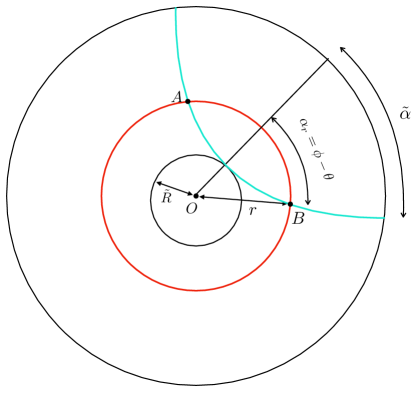
Figure 5: A spacelike geodesic (in turquoise) at a time slice in conical or pure AdS centered at boundary angular coordinate $\theta$ and with a boundary opening angle $\tilde{\alpha}$. The geodesic is by construction tangent to a bulk disk of radius $\tilde{R}$. The geodesic distance between points $A$ and $B$, which both lie on a circle (in red) of radius $r$, is computed in appendix B.2.

Consider a spacelike geodesic at a constant time slice in conical AdS (93), which is centered at the boundary angular coordinate $\theta$ and which has boundary opening angle $\tilde{\alpha}$ (see figure 5 for notational clarifications). The geodesic distance functional is

$$I=\int ds=\int dr\sqrt{\frac{1}{\gamma^{2}+(r/L)^{2}}+r^{2}\left(\frac{d\phi}{dr}\right)^{2}}.$$ (190)

Minimizing the geodesic distance yields

$$\frac{r^{2}\dot{\phi}}{\sqrt{\left(\gamma^{2}+(r/L)^{2}\right)^{-1}+r^{2}\dot{\phi}^{2}}}=\text{constant},$$ (191)

where the dot denotes differentiation with respect to the radial coordinate $r$. The constant is fixed by noting that the geodesic has a turning point, at $r=\tilde{R}$, where the derivative diverges, i.e. $\dot{\phi}\to\infty$ as $r\to\tilde{R}$. Plugging the resulting constant, $\tilde{R}$, into (191) leads to the following differential equation

$$\frac{d\phi}{dr}=\frac{\tilde{R}L}{r\sqrt{(r^{2}-\tilde{R}^{2})\left(r^{2}+\gamma^{2}L^{2}\right)}}\,.$$ (192)

By integrating this equation between the turning point $(r=\tilde{R},\phi=\theta)$ and an arbitrary point on the geodesic $(r,\theta+\alpha_{r})$, where $\alpha_{r}$ is the opening angle in the bulk, we arrive at the following expression for the geodesics

$$\tan^{2}(\gamma\alpha_{r})=\frac{r^{2}/\tilde{R}^{2}-1}{r^{2}/(\gamma L)^{2}+1}\,.$$ (193)

Note that in the limit $r\to\infty$ the bulk opening angle $\alpha_{r}$ becomes the boundary opening angle $\tilde{\alpha}$ (both range from $0$ to $\pi/2$). Hence, by taking the limit $r\to\infty$ of the equation above, we find a relation between the radius of the disk and the boundary opening angle

$$\tilde{R}=L\gamma\cot(\gamma\tilde{\alpha})\,.$$ (194)

In terms of $\tilde{\alpha}$, instead of $\tilde{R}$, the geodesic equation reads

$$\tan^{2}(\gamma\alpha_{r})=\frac{r^{2}\tan^{2}(\gamma\tilde{\alpha})-\gamma^{2}L^{2}}{r^{2}+\gamma^{2}L^{2}}\qquad\text{or}\qquad\frac{r}{\sqrt{r^{2}+\gamma^{2}L^{2}}}\cos(\gamma\alpha_{r})=\cos(\gamma\tilde{\alpha}).$$ (195)

These results agree with the expressions in Balasubramanian:2014sra , which were derived by rescaling the coordinates in the pure AdS case. According to (92) the coordinate transformation from pure AdS to conical AdS is $\phi^{\prime}=\phi\gamma$ and $r^{\prime}=r/\gamma$. Applying this transformation to the geodesic equation in pure AdS gives the required results.

In the main body of this paper we have used several special cases of this general set-up (also in pure AdS, with $\gamma=1$), such as $r=R>\tilde{R}$ (with $\alpha_{r}\to\alpha_{R}$) in equations (17) and (25), and $r=R=\tilde{R}$ (in which case $\tilde{\alpha}\to\alpha$ and $\alpha_{R}\to 0$) in equations (26) and (107).

B.2 Chord length

From the embedding formalism: Given the embedding coordinates defined in appendix A, one can derive an expression for the geodesic length. It is convenient to combine the embedding coordinates into a vector $X^{\alpha}=(T^{1},T^{2},X^{1},X^{2})$ and use the following notation for the inner product $X^{2}=g_{\alpha\beta}X^{\alpha}X^{\beta}$ and $X_{1}\cdot X_{2}=g_{\alpha\beta}X_{1}^{\alpha}X_{2}^{\beta},$ where the embedding metric is given by (170).

The Lagrangian in embedding space which describes geodesics in AdS is

$$\mathcal{L}=\frac{1}{2}\dot{X}^{2}+\mu(X^{2}+L^{2}),$$ (196)

where the dot indicates differentiation with respect to the proper distance $s$, and a Lagrange multiplier $\mu$ is introduced to ensure that the geodesics are confined to the hyperboloid (171). The Euler-Lagrange equation is $\ddot{X}^{\alpha}=2\mu X^{\alpha}.$ Combining this with the hyperboloid constraint $X^{2}=-L^{2}$ yields an expression for the Lagrange multiplier $\mu=\dot{X}^{2}/(2L^{2}).$ Therefore, geodesics in AdS satisfy a simple equation in embedding space

$$L^{2}\ddot{X}^{\alpha}=\dot{X}^{2}X^{\alpha}.$$ (197)

The general solution for spacelike geodesics ($\dot{X}^{2}=1$) is

$$X^{\alpha}(s)=m^{\alpha}e^{s/L}+n^{\alpha}e^{-s/L},$$ (198)

where $m^{\alpha}$ and $n^{\alpha}$ are constant vector that obey $m^{2}=n^{2}=0$ and $2m\cdot n=-L^{2}.$ By taking the inner product between two points $X(s_{1})$ and $X(s_{2})$, we arrive at the following formula for the geodesic distance or chord length $\lambda:=s_{2}-s_{1}$,

$$L^{2}\cosh\left(\frac{\lambda}{L}\right)=-X(s_{1})\cdot X(s_{2}).$$ (199)

We can now compute the chord length for pure AdS and conical AdS by inserting specific embedding coordinates. In the standard coordinates $(t,r,\phi)$ for pure AdS the geodesic length between the two bulk points $A=(0,r,\theta-\alpha_{r})$ and $B=(0,r,\theta+\alpha_{r})$ is (see figure 5)

$$\lambda_{\text{vac}} =L\,\text{arccosh}\left[1+2\,(r/L)^{2}\,\sin^{2}(\alpha_{r})\right]=2L\operatorname{arcsinh}[(r/L)\sin(\alpha_{r})]$$ (200)

$$=2L\operatorname{arctanh}\left[\frac{(r/L)\sin(\alpha_{r})}{\sqrt{1+(r/L)^{2}\sin^{2}(\alpha_{r})}}\right]\,.$$

A similar calculation using the embedding coordinates (184) for conical AdS shows

$$\lambda_{\text{con}} =L\,\text{arccosh}\left[1+2\,r^{2}/(\gamma L)^{2}\,\sin^{2}(\gamma\alpha_{r})\right]=2L\operatorname{arcsinh}\left[r/(\gamma L)\sin(\gamma\alpha_{r})\right]$$ (201)

$$=2L\operatorname{arctanh}\left[\frac{r/(\gamma L)\sin(\gamma\alpha_{r})}{\sqrt{1+r^{2}/(\gamma L)^{2}\sin^{2}(\gamma\alpha_{r})}}\right].$$

In other words, the conical AdS result for a disk of radius $r$ is obtained from the pure AdS case by replacing $r\to r/\gamma$ and $\alpha_{r}\to\gamma\alpha_{r}$.

From the kinematic space formalism:

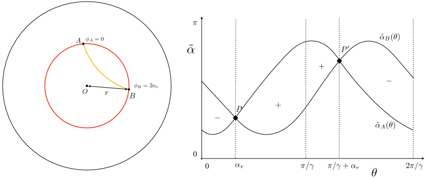
Figure 6: Left diagram: geodesic arc (in yellow) on a constant time slice of conical AdS between two points $A$ and $B$ on a circle (in red) of radius $r$ and with angular coordinates $\phi_{A}=0$ and $\phi_{B}=2\alpha_{r}$. For simplicity, the conical parameter $\epsilon=1-\gamma$ is taken to be much smaller than one, so the geodesics take a similar form as those in pure AdS. Right diagram: kinematic space $(\theta,\tilde{\alpha})$ with point curves $\tilde{\alpha}_{A}(\theta)$ and $\tilde{\alpha}_{B}(\theta)$ corresponding to the two bulk points in the left diagram. The geodesic distance between $A$ and $B$ is computed by an integral in kinematic space over the region $\Delta_{AB}$ enclosed by the two point curves.

An alternative way to derive the chord length between two bulk points $A$ and $B$ is from the integral of the Crofton form over kinematic space Czech:2015qta

$$\frac{\lambda(A,B)}{4G}=\frac{1}{4}\int_{\Delta_{AB}}\omega(\theta,\tilde{\alpha}).$$ (202)

In this appendix we parametrize kinematic space with the pair $(\theta,\tilde{\alpha})$, where $\theta$ is the center of a spatial boundary region and $2\tilde{\alpha}$ is the angular size of the region (see figure 5). The Crofton form $\omega$ is the volume form on kinematic space, and the integration region $\Delta_{AB}$ is the region in kinematic space between the two point curves $\tilde{\alpha}_{A}(\theta)$ and $\tilde{\alpha}_{B}(\theta)$ associated to the bulk points $A$ and $B$, respectively. We recall that a point curve $\tilde{\alpha}_{p}(\theta)$ is formed by all geodesics on a constant time slice in AdS that intersect a bulk point $p$. The region $\Delta_{AB}$ corresponds in the bulk to the set of all geodesics which intersect the geodesic arc between the points $A$ and $B$ (see figure 6).

Using the expression for the Crofton form in terms of the entanglement entropy (14), and $c=3L/(2G)$, we can also write the chord length as

$$\lambda=-\frac{3L}{4c}\int_{0}^{2\pi}d\theta\,\partial_{\tilde{\alpha}}S(\tilde{\alpha})\Big{|}_{\tilde{\alpha}_{B}(\theta)}^{\tilde{\alpha}_{A}(\theta)}.$$ (203)

Here we employed Stokes’ theorem to remove the integration over $\tilde{\alpha}$. We would like to compute the chord length between two points $A$ and $B$ in conical AdS space, which lie on a circle of radius $r$. The pure AdS case can be obtained by setting $\gamma=1$ at every step. Suppose the bulk angular coordinates are given by $\phi_{A}=0$ and $\phi_{B}=2\alpha_{r}$. Then, it follows from (195) that the point curves of $A$ and $B$ satisfy the following equations

$$\tilde{\alpha}_{A}(\theta) =\frac{1}{\gamma}\arccos\left[\frac{r}{\sqrt{r^{2}+\gamma^{2}L^{2}}}\cos(\gamma\theta)\right]$$ (204)

$$\tilde{\alpha}_{B}(\theta) =\frac{1}{\gamma}\arccos\left[\frac{r}{\sqrt{r^{2}+\gamma^{2}L^{2}}}\cos[\gamma(\theta-2\alpha_{r})]\right].$$

The two point curves intersect themselves, i.e. $\tilde{\alpha}_{A}(\theta)=\tilde{\alpha}_{B}(\theta)$, at two points in kinematic space given by $P=\{\theta=\alpha_{r}\}$ and $P^{\prime}=\{\theta=\pi/\gamma+\alpha_{r}\}$. These two points are depicted in the right diagram of figure 6 and they denote a unique geodesic in the bulk passing through both the points $A$ and $B$. The only difference between $P$ and $P^{\prime}$ is that the orientation of the geodesic is opposite for these two points.

The entanglement entropy of an excited state in a CFT dual to conical AdS is given by $S^{\text{con}}(\tilde{\alpha})=\frac{c}{3}\log\left[2L/(\mu\gamma)\sin(\gamma\tilde{\alpha})\right]$, cf. equation (48), where $\mu$ is a UV cutoff and $L$ is the radius of the cylinder, and hence its derivative is

$$\partial_{\tilde{\alpha}}S^{\text{con}}(\tilde{\alpha})=\gamma\frac{c}{3}\frac{\cos(\gamma\tilde{\alpha})}{\sin(\gamma\tilde{\alpha})}.$$ (205)

Plugging this into (203) yields that the contributions from the two point curves $\tilde{\alpha}_{A}$ and $\tilde{\alpha}_{B}$ are equal due to the circular symmetry of the setup. Further, to account for the orientation of the geodesics, we need to add appropriate signs for the four different integration regions inside $\Delta_{AB}$ (see figure 6 for our sign convention). The chord length thus consists of four different integrals

$$\lambda_{\text{con}}=-\frac{\gamma L}{2}\left[-\int_{0}^{\alpha_{r}}+\int_{\alpha_{r}}^{\pi/\gamma}+\int_{\pi/\gamma}^{\pi/\gamma+\alpha_{r}}-\int_{\pi/\gamma+\alpha_{r}}^{2\pi/\gamma}\right]d\theta\,\frac{\cos(\gamma\tilde{\alpha})}{\sin(\gamma\tilde{\alpha})}\Bigg{|}_{\tilde{\alpha}_{A}(\theta)}.$$ (206)

The transformation $\theta\to\theta+\pi/\gamma$ reverses the orientation of the geodesics, and it flips the sign of the integrand. This implies that the first and third integral, and the second and fourth integral, give the same result. The first and second integral are also the same, since the integral vanishes for the values $\theta=0$ and $\theta=\pi/\gamma$. The four different integrals are therefore all equal, and hence after rewriting the integrand we find

$$\lambda_{\text{con}}=2\gamma L\int_{0}^{\alpha_{r}}d\theta\frac{x(\theta)}{\sqrt{1-x^{2}(\theta)}}\qquad\text{with}\qquad x(\theta)=\frac{r}{\sqrt{r^{2}+\gamma^{2}L^{2}}}\cos(\gamma\theta).$$ (207)

Finally, this integral yields the same expression for the chord length as (201)

$$\lambda_{\text{con}}=2L\operatorname{arctanh}\left[\frac{r/(\gamma L)\sin(\gamma\alpha_{r})}{\sqrt{1+r^{2}/(\gamma L)^{2}\sin^{2}(\gamma\alpha_{r})}}\right].$$ (208)

Appendix C Conformal isometry of causal diamonds on the cylinder

The conformal isometry of a causal diamond in Minkowski space is well studied in the literature Casini:2011kv ; Faulkner:2013ica ; Jacobson:2015hqa . However, Minkowski space corresponds to the conformal boundary of the Poincaré patch of AdS, whereas in the present paper we work in global AdS, whose conformal boundary is a (Lorentzian) cylinder. In this appendix we derive the conformal Killing vector generating the conformal isometry that preserves a causal diamond on the two-dimensional cylinder in two distinct ways: from the generators of the conformal group and from the boundary limit of the boost Killing vector of Rindler-AdS₃.

C.1 From the conformal group

On the complex plane the generators of the global conformal group are $\partial_{z},\partial_{\bar{z}}$ which generate translations, $z\partial_{z},\bar{z}\partial_{\bar{z}}$ which generate dilatations and rotations, and $z^{2}\partial_{z},\bar{z}^{2}\partial_{\bar{z}}$ which generate special conformal transformations. These generators can be mapped to the generators of the conformal group on the cylinder by the conformal transformation $\omega=i\log z$, where $\omega=\theta+i\tau_{E}$ parametrizes the (Euclidean) cylinder. The line element transforms as $dzd\bar{z}=e^{i(\bar{\omega}-\omega)}d\omega d\bar{\omega}=e^{2\tau_{E}}(d\tau_{E}^{2}+d\theta^{2})$. Since a conformal generator remains a generator of the conformal group after a Weyl rescaling of the metric, we can safely ignore the conformal factor. The basis of conformal generators on the cylinder is thus given by

$$\{e^{-i\omega}\partial_{\omega},\,\,\partial_{\omega},\,\,e^{i\omega}\partial_{\omega}\}\cup\left\{\omega\to\bar{\omega}\right\}.$$ (209)

In Lorentzian signature the complex coordinate is $\omega=\theta-\tau$ and its complex conjugate is $\bar{\omega}=\theta+\tau$, where $\tau=-i\tau_{E}$ is the Lorentzian time. Together $\omega$ and $\bar{\omega}$ form a null coordinate system on the cylinder. In the following, however, we take the null coordinates to be the retarded and advanced times $u=\tau-\theta$ and $v=\tau+\theta$, since they are both increasing towards the future. We write the basis of generators now in terms of trigonometric functions of these null coordinates

$$\{\partial_{u},\sin u\,\partial_{u},\cos u\,\partial_{u}\}\cup\left\{u\to v\right\}.$$ (210)

The Killing vector fields $\partial_{u}+\partial_{v}$ and $-\partial_{u}+\partial_{v}$, respectively, generate time translations and rotations on the cylinder, and the other four basis vectors are conformal Killing vectors which do not generate isometries of the metric $-dudv$.

We put the origin of the null coordinate system, $u=v=0$, at the center of the causal diamond. The lines $u=\pm\alpha$ and $v=\pm\alpha$ are the null boundaries of the diamond. Since the diamond has a reflection symmetry across the $u=v$ line (the $t$-axis), the conformal isometry that preserves the diamond must be invariant under the exchange of $u$ and $v$. The conformal Killing vector which generates this conformal isometry therefore takes the general form

$$\xi=A(u)\partial_{u}+A(v)\partial_{v},$$ (211)

$$\text{with}\quad A(u)=a+b\sin u+c\cos u.$$

To remain inside the diamond the flow of $\xi$ must leave the vertices $u=v=\pm\alpha$ and the edge $v=-u=\alpha$ of the diamond fixed. This requirement yields $A(\pm\alpha)=0$, which determines the function up to a normalization: $A(u)=c\left(\cos u-\cos\alpha\right).$ The normalization is fixed by demanding that the surface gravity of $\xi$ is equal to one, $\kappa=-A^{\prime}(\alpha)=c\sin\alpha=1$, at the future null boundary of the diamond. Thus, the conformal Killing vector whose flow preserves a causal diamond on the cylinder, and which has unit surface gravity, is in terms of null coordinates

$$\xi=\frac{1}{\sin\alpha}\Big{[}\left(\cos u-\cos\alpha\right)\partial_{u}+\left(\cos v-\cos\alpha\right)\partial_{v}\Big{]}.$$ (212)

In terms of the $\tau$ and $\theta$ coordinates on the Lorentzian cylinder, $\xi$ becomes

$$\xi=\frac{1}{\sin\alpha}\Big{[}\left(\cos\tau\cos\theta-\cos\alpha\right)\,\partial_{\tau}-\sin\tau\sin\theta\,\partial_{\theta}\Big{]}.$$ (213)

As a limiting case, note that for small diamonds, i.e. $u,v,\alpha\ll 1$, $\xi$ reduces to the expression in flat space Faulkner:2013ica ; Jacobson:2015hqa

$$\xi =\frac{1}{2\alpha}\left[\left(\alpha^{2}-u^{2}\right)\partial_{u}+\left(\alpha^{2}-v^{2}\right)\partial_{v}\right].$$ (214)

An illustration of $\xi$ is given in figure 7, where we have also indicated the boost Killing vector of the associated Rindler wedge in the bulk. We will discuss the latter in the following section.

C.2 From the boundary limit of the boost Killing vector

The conformal isometry that preserves a causal diamond on the Lorentzian cylinder can also be obtained from the boundary limit of a proper isometry of AdS space. This is because the conformal Killing vector $\xi$ of a causal diamond in flat space extends to the boost Killing vector $\chi$ of the Rindler wedge of AdS space (see figure 7). The boost Killing vector generates proper time translations for uniformly accelerating (Rindler) observers in AdS with $a>L^{-1}$. The vector field $\chi$ takes quite a simple form in Poincaré coordinates Faulkner:2013ica , but is slightly more complicated in global AdS coordinates, as we will see below. We need the expression for $\chi$ in global coordinates, since its boundary limit yields the conformal Killing vector of a diamond on the cylinder, which is the conformal boundary of global AdS.

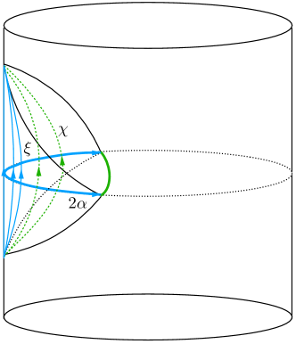
Figure 7: The Rindler wedge of pure AdS₃ with associated boundary causal diamond (in black). The bifurcation surface (in green) of the AdS-Rindler horizon is the Ryu-Takayanagi surface associated to the entangling region of angular size $2\alpha$ (in blue). The boost Killing vector $\chi$ (with flow in green) of AdS-Rindler asymptotes to the conformal Killing vector $\xi$, which generates a flow (in blue) inside the boundary causal diamond.

It is straightforward to derive the Killing vectors of AdS from the embedding space (see appendix A). The isometry group of $\text{AdS}_{3}$, $SO(2,2)$, is generated by six linearly independent Killing vectors in the embedding space $\mathbb{R}^{2,2}$: two generators of rotations and four generators of boosts. The boost Killing vector of the AdS-Rindler wedge corresponds to the Killing vector associated with a boost in the $(T^{2},X^{1})$ plane of the embedding space. This is because the embedding coordinates $T^{2}$ and $X^{1}$ for AdS-Rindler space, in equation (176), parametrize a Rindler observer (or hyperbola) in embedding space, with proper time $\sigma=L\,\text{arctanh}(T^{2}/X^{1})$ and proper distance $\varrho=\sqrt{(X^{1})^{2}-(T^{2})^{2}}$. Rindler observers in embedding space are therefore in one-to-one correspondence with Rindler observers in AdS Deser:1997ri . Indeed, the Killing vector which generates a boost in the $(T^{2},X^{1})$ plane of embedding space, $B=X^{1}\partial_{T^{2}}+T^{2}\partial_{X^{1}}$, becomes the generator of $\sigma$-time translations in AdS-Rindler space, i.e. $B=L\partial_{\sigma}$.

Next, we compute the boost Killing vector in the global coordinates (172) for AdS

$$B=\!\frac{rL}{\sqrt{L^{2}+r^{2}}}\cos(t/L)\cos\phi\partial_{t}+\sqrt{L^{2}+r^{2}}\sin(t/L)\cos\phi\,\partial_{r}-\frac{\sqrt{L^{2}+r^{2}}}{r}\sin(t/L)\sin\phi\,\partial_{\phi}.$$ (215)

The boost Killing vector becomes null on the AdS-Rindler horizon, which in global coordinates is described by $\{\cos(t/L\pm\pi/2)=\frac{r}{\sqrt{r^{2}+L^{2}}}\cos\phi\}$, and vanishes at the boundary vertices $\{t=\pm\pi L/2,r=\infty,\phi=0\}$ and at the straight line $\{t=0,\phi=\pi/2,3\pi/2\}$. Note that the straight line, which is the bifurcation surface of the horizon, cuts the $t=0$ time slice of AdS in two wedges of equal size, since each wedge subtends an angle $\pi$. In other words, the left and right AdS-Rindler wedges both cover half of the boundary cylinder at $t=0$. This is also manifest from the boundary limit $r\to\infty$ of the boost Killing vector, which equals (213) only for $\alpha=\pi/2$. Hence, we have not yet found the extension into the bulk of the most general boundary conformal Killing vector $\xi$, which should hold for any $\alpha$.

Fortunately, we can move the bifurcation surface of the horizon by an isometry of AdS to a new position that intersects the boundary at $\phi=\alpha$ and $\phi=2\pi-\alpha$. The new bifurcation surface subtends an angle $2\alpha$ at the boundary, instead of $\pi$ as in the previous case. A simple isometry that relates different bifurcation surfaces (and hence different AdS-Rindler wedges) is a boost in the $(T^{1},X^{1})$ plane of embedding space Casini:2011kv . This boost transforms the embedding coordinates as

$$(T^{1})^{\prime} =\cosh\beta\,T^{1}-\sinh\beta\,X^{1},$$ (216)

$$(X^{1})^{\prime} =\cosh\beta\,X^{1}-\sinh\beta\,T^{1},$$

where $\beta$ is an arbitrary rapidity parameter which ranges from $-\infty$ to $\infty$. The boost Killing vector of the transformed AdS-Rindler wedge is now given by the boost generator in the $(T^{2},(X^{1})^{\prime})$ plane

$$\chi=(X^{1})^{\prime}\partial_{T^{2}}+T^{2}\partial_{(X^{1})^{\prime}}.$$ (217)

By substituting $T^{1}$ and $X^{1}$ in (176) with $(T^{1})^{\prime}$ and $(X^{1})^{\prime}$, respectively, the induced metric for the new AdS-Rindler wedge is identical to the one given by equation (177), and the boost Killing vector remains equal to

$$\chi=L\partial_{\sigma}$$ (218)

in AdS-Rindler coordinates. Relative to global coordinates, however, the AdS-Rindler wedge has been displaced by the boost (216), since we use the same embedding coordinates for global AdS as before performing the boost. Hence in global coordinates the new boost Killing vector (217) takes a different form compared to the one in equation (215). In order to derive this form, we first express the boost Killing vector in terms of the unprimed embedding coordinates

$$\chi =\cosh\beta\,B-\sinh\beta\,H,\quad\text{with}$$ (219)

$$B=X^{1}\partial_{T^{2}}+ T^{2}\partial_{X^{1}}\quad\text{and}\quad H=T^{1}\partial_{T^{2}}-T^{2}\partial_{T^{1}}.$$ (220)

Here $H$ generates rotations in the $(T^{1},T^{2})$ plane. We would like to express $\chi$, however, in terms of the boundary opening angle $\alpha$ instead of the rapidity $\beta$. Their relation can be derived as follows. By inverting the boost (216) and plugging in the embedding coordinates $(T^{1})^{\prime}=\sqrt{\varrho^{2}+L^{2}}\cosh(u/L)$ and $(X^{1})^{\prime}=\varrho\cosh(\sigma/L)$, we find

$$T^{1} =\cosh\beta\,\sqrt{\varrho^{2}+L^{2}}\cosh(u/L)+\sinh\beta\,\varrho\cosh(\sigma/L),$$ (221)

$$X^{1} =\cosh\beta\,\varrho\cosh(\sigma/L)+\sinh\beta\,\sqrt{\varrho^{2}+L^{2}}\cosh(u/L).$$

The transformation between the AdS-Rindler and the global coordinate system can be found by inserting the embedding coordinates $T^{1}$ and $X^{1}$ for global AdS given by (172) into these equations, and identifying the other two (not boosted) embedding coordinates $T^{2}$ and $X^{2}$ for global AdS with those for AdS-Rindler space given by (176). The resulting coordinate transformation is

$$\tan(t/L) =\frac{\varrho\sinh(\sigma/L)}{\cosh\beta\,\sqrt{\varrho^{2}+L^{2}}\cosh(u/L)+\sinh\beta\,\varrho\cosh(\sigma/L)},$$

$$\tan\phi =\frac{\sqrt{\varrho^{2}+L^{2}}\sinh(u/L)}{\cosh\beta\,\varrho\cosh(\sigma/L)+\sinh\beta\,\sqrt{\varrho^{2}+L^{2}}\cosh(u/L)},$$ (222)

$$r^{2} =\left(\cosh\beta\,\varrho\cosh(\sigma/L)+\sinh\beta\,\sqrt{\varrho^{2}+L^{2}}\cosh(u/L)\right)^{2}+\left(\varrho^{2}+L^{2}\right)\sinh^{2}(u/L).$$

The time slice $\sigma=0$ corresponds to $t=0$ in global coordinates. The bifurcation surface of the horizon lies inside that time slice and intersects the asymptotic boundary at $u/L=\infty$ in AdS-Rindler coordinates, and at $\phi=\alpha$ and $\phi=2\pi-\alpha$ in global coordinates. The relation between $\beta$ and $\alpha$ thus follows from evaluating the second equation at $\sigma=0$ and taking the limit $\varrho/L\to\infty$ and, subsequently, $u/L\to\infty$, i.e.

$$\cosh\beta=\frac{1}{\sin\alpha}\qquad\text{and}\ \qquad\sinh\beta=\frac{1}{\tan\alpha}\,,$$ (223)

where $\beta$ now ranges from $0$ to $\infty$, and we still have $0\leq\alpha\leq\pi/2$. As a function of $\alpha$ the boost Killing vector (219) is hence given by

$$\chi=\frac{1}{\sin\alpha}\big{(}B-\cos\alpha\,H\big{)}.$$ (224)

Note that for $\alpha=\pi/2$ (or $\beta=0$) the boost Killing vector reduces to $\chi=B$. In global AdS coordinates the Killing vector $H$ is simply the generator of time translations $H=L\partial_{t}$, whereas $B$ is given by (215). Therefore, in global coordinates we find

$$\chi= \frac{1}{\sin\alpha}\!\Bigg{[}\!\left(\frac{rL}{\sqrt{L^{2}+r^{2}}}\cos(t/L)\cos\phi-L\cos\alpha\right)\partial_{t}+\sqrt{L^{2}+r^{2}}\sin(t/L)\cos\phi\,\partial_{r}$$ (225)

$$\qquad\,\,-\frac{\sqrt{L^{2}+r^{2}}}{r}\sin(t/L)\sin\phi\,\partial_{\phi}\Bigg{]}.$$

One can readily verify that the vertices $\{t=\pm\alpha L,r=\infty,\phi=0\}$ of the boundary causal diamond and the extremal surface $\{t=0,\cos\alpha=\frac{r}{\sqrt{r^{2}+L^{2}}}\cos\phi\}$ are fixed points of the flow of $\chi$. The extremal surface is the bifurcation surface of the horizon. Further, $\chi$ becomes null on the past and future Killing horizon, which are given by $\{\cos(t/L\pm\alpha)=\frac{r}{\sqrt{r^{2}+L^{2}}}\cos\phi\}$ in global coordinates or $\varrho=0$ in AdS-Rindler coordinates. The normalization of $\chi$ is such that the surface gravity is unity, $\kappa=1$, at the future horizon. Furthermore, let us stress that under the mapping (C.2) the boost Killing field above turns into $L\partial_{\sigma}.$

In terms of the dimensionless sausage coordinates (175) the boost generator reads

$$\chi=\frac{1}{\sin\alpha}\!\left[\!\left(\frac{2z}{1+z^{2}}\cos\tau\cos\phi-\cos\alpha\right)\partial_{\tau}+\frac{1-z^{2}}{2}\sin\tau\cos\phi\,\partial_{z}-\frac{1+z^{2}}{2z}\sin\tau\sin\phi\,\partial_{\phi}\right],$$ (226)

and in terms of the spherical coordinates (181) the boost Killing vector is simply

$$\chi=\frac{1}{\sin\alpha}\!\left[\Big{(}\cos\hat{\tau}\cos\hat{\phi}-\cos\alpha\Big{)}\partial_{\hat{\tau}}-\sin\hat{\tau}\sin\hat{\phi}\partial_{\hat{\phi}}\right].$$ (227)

Surprisingly, this is independent of the bulk angular coordinate $\psi$, and hence the expression does not change in the asymptotic limit $\psi\to 0$ or $\pi$. The boundary limit $r\to\infty$ and $z\to 1$ of the other expressions for $\chi$, respectively (225) and (226), yield the same result for the associated conformal Killing vector on the boundary cylinder

$$\xi=\lim_{\text{bndy}}\chi=\frac{1}{\sin\alpha}\Big{[}\left(\cos\tau\cos\theta-\cos\alpha\right)\partial_{\tau}-\sin\tau\sin\theta\,\partial_{\theta}\Big{]}.$$ (228)

As expected, this matches with expression (213) for the conformal Killing vector which generates the conformal isometry of a causal diamond on the boundary cylinder. Note that we expressed $\xi$ in terms of the dimensionless boundary coordinates $\tau$ and $\theta$. Although we have focussed on a three-dimensional bulk spacetime in this appendix, the equations above for the boost Killing vector of AdS-Rindler space (and its corresponding boundary limit) are also valid in higher dimensions. This is because the expression (219) for $\chi$ in embedding coordinates remains the same.

Finally, for completeness, let us check that the embedding expression reproduces the boost Killing vector in Poincaré coordinates (178). The rotation and boost generators are

$$B =\frac{1}{2L}\left[(L^{2}-\mathrm{t}^{2}-\mathrm{x}^{2}-\mathrm{z}^{2})\partial_{\mathrm{t}}-2\mathrm{t}(\mathrm{x}\partial_{\mathrm{x}}+\mathrm{z}\partial_{\mathrm{z}})\right],$$ (229)

$$H =\frac{1}{2L}\left[(L^{2}+\mathrm{t}^{2}+\mathrm{x}^{2}+\mathrm{z}^{2})\partial_{\mathrm{t}}+2\mathrm{t}(\mathrm{x}\partial_{\mathrm{x}}+\mathrm{z}\partial_{\mathrm{z}})\right].$$

The rapidity $\beta$ is in this case related to the radius $R$ of a sphere at $\mathrm{t}=0$ in the flat boundary space via $R=e^{-\beta}L$ Casini:2011kv . Combining this relation with (219) and (229), we recover the known expression for the boost Killing vector in Poincaré coordinates Faulkner:2013ica

$$\chi =\frac{L}{2R}\left[\left(1+(R/L)^{2}\right)B-\left(1-(R/L)^{2}\right)H\right]$$ (230)

$$=\frac{1}{2R}\left[\left(R^{2}-\mathrm{t}^{2}-\mathrm{x}^{2}-\mathrm{z}^{2}\right)\partial_{\mathrm{t}}-2\mathrm{t}\mathrm{x}\partial_{\mathrm{x}}-2\mathrm{t}\mathrm{z}\partial_{\mathrm{z}}\right].$$

Note that the term involving $H$ in the first equation is only nonzero if the radius of the sphere is not equal to the AdS radius (see also appendix D in Jacobson:2018ahi ). The transformation between Poincaré coordinates and AdS-Rindler coordinates, which maps the boost Killing vector (230) to the time translation generator (218), can be obtained in a similar fashion as the transformation (C.2) for global coordinates above (see for instance equation (80) in Espindola:2018ozt ).

Appendix D Variation of coupling constants in the first law of causal diamonds

In this section we compute the contributions of the variation of gravitational coupling constants in the first law of causal diamonds in maximally symmetric spacetimes. We consider variations of both the cosmological constant and Newton’s constant, and prove that terms proportional to the variation of Newton’s constant cancel out in the first law. We employ the covariant phase space method Wald:1993nt ; Iyer:1994ys , which has been extended in Urano:2009xn ; Caceres:2016xjz to include variations of couplings, and we follow the notation of Jacobson:2018ahi .

Suppose $L(\phi,\alpha_{i})=\mathcal{L}(\phi,\alpha_{i})\epsilon$ is a diffeomorphism invariant Lagrangian $d$-form that depends on the dynamical fields $\phi$ and coupling constants $\alpha_{i}$. If one allows for variations of coupling constants $\alpha_{i}$, then the on-shell fundamental variational identity in the covariant phase space formalism becomes

$$\delta H_{\zeta}=\oint_{\partial D}\delta Q_{\zeta}+\int_{D}\zeta\cdot E^{\alpha_{i}}\delta\alpha_{i}.$$ (231)

Here $\zeta$ is the conformal Killing vector of a maximally symmetric causal diamond, $H_{\zeta}$ is the Hamiltonian generating evolution along the flow of $\zeta$, $Q_{\zeta}$ is the associated Noether charge $(d-2)$-form, and the $d$-form $E^{\alpha_{i}}=(\partial\mathcal{L}/\partial\alpha_{i})\epsilon$ is the derivative of the Lagrangian with respect to the coupling $\alpha_{i}$.

Assuming minimal coupling, the Lagrangian uniquely splits into a gravitational and a matter part: $L=L^{\text{grav}}+L^{\text{mat}}$. We consider the gravitational Lagrangian for general relativity plus a cosmological constant

$$L^{\text{grav}}=\frac{R-2\Lambda}{16\pi G}\epsilon.$$ (232)

We only take variations of the gravitational coupling constants $\alpha_{i}=\{\Lambda,G\}$ into account in the first law, and not of the matter couplings. The derivatives of the gravitational Lagrangian with respect to $\Lambda$ and $G$ are

$$E^{\Lambda}=-\frac{\epsilon}{8\pi G}\qquad\text{and}\qquad E^{G}=-\frac{R-2\Lambda}{16\pi G^{2}}\epsilon=-\frac{\Lambda}{(d-2)4\pi G^{2}}\epsilon,$$ (233)

where we evaluated the Ricci scalar on the maximally symmetric background in the last equality. For Einstein gravity the fundamental identity thus takes the form

$$\delta H_{\zeta}=\oint_{\partial D}\delta Q_{\zeta}-\frac{1}{8\pi G}\left(\delta\Lambda+\frac{2\Lambda}{d-2}\frac{\delta G}{G}\right)\int_{D}\zeta\cdot\epsilon.$$ (234)

The integral of $\zeta\cdot\epsilon$ over the disk can be identified with the thermodynamic volume $V_{\zeta}$ (146). Further, the Noether charge variation is given by

$$\oint_{\partial D}\delta Q_{\zeta}=-\frac{\kappa}{8\pi}\delta\left(\frac{A}{G}\right),$$ (235)

where Newton’s constant is included in the variation. The Hamiltonian variation splits into a gravitational and matter part, $\delta H_{\zeta}=\delta H_{\zeta}^{\text{grav}}+\delta H_{\zeta}^{\text{mat}}$, with the gravitational part defined as the symplectic form evaluated on the Lie derivative of the metric along $\zeta$

$$\delta H_{\zeta}^{\text{grav}}=\int_{D}\omega(g,\delta g,\mathcal{L}_{\zeta}g)=\int_{D}\left[\delta\theta(g,\mathcal{L}_{\zeta}g)-\mathcal{L}_{\zeta}\theta(g,\delta g)\right].$$ (236)

Here $\theta$ is the so-called symplectic potential $(d-1)$-form. The Hamiltonian variation contains contributions from both the variation of the metric and the variation of Newton’s constant, $\delta H_{\zeta}^{\text{grav}}=\delta_{g}H_{\zeta}^{\text{grav}}+\delta_{G}H_{\zeta}^{\text{grav}}$, which are given by

$$\delta_{g}H_{\zeta}^{\text{grav}}=-\frac{\kappa k}{8\pi G}\delta V\quad\text{and}\quad\delta_{G}H_{\zeta}^{\text{grav}}=\int_{D}\delta_{G}\theta(g,\mathcal{L}_{\zeta}g)=-\frac{d-1}{d-2}\,\frac{\kappa k}{8\pi}\,V\delta\!\left(\frac{1}{G}\right).$$ (237)

This follows respectively from equations (3.35) and (3.9) in Ref. Jacobson:2018ahi . Therefore, plugging (235) and (237) into the fundamental identity, we find a first law which includes variations of both $\Lambda$ and $G$

$$\delta H_{\zeta}^{\text{mat}}-\frac{\kappa k}{8\pi G}\left(\delta V-\frac{d-1}{d-2}\,V\,\frac{\delta G}{G}\right)=-\frac{\kappa}{8\pi G}\,\delta A+\frac{\kappa A}{8\pi G}\,\frac{\delta G}{G}-\frac{V_{\zeta}}{8\pi G}\left(\delta\Lambda+\frac{2\Lambda}{d-2}\frac{\delta G}{G}\right).$$ (238)

However, we can deduce from the Smarr formula (160),

$$(d-1)\kappa kV=(d-2)\kappa A-2V_{\zeta}\Lambda,$$ (239)

that the terms involving the variation of Newton’s constant cancel each other. Thus, the final form of the first law of causal diamonds is

$$\delta H_{\zeta}^{\text{mat}}-\frac{\kappa k}{8\pi G}\delta V=-\frac{\kappa}{8\pi G}\delta A-\frac{V_{\zeta}}{8\pi G}\delta\Lambda,$$ (240)

which agrees with the result in Jacobson:2018ahi .

References

- (1) J. D. Bekenstein, Black holes and entropy, Phys. Rev. D 7 (1973) 2333–2346.
- (2) J. M. Bardeen, B. Carter, and S. Hawking, The Four laws of black hole mechanics, Commun. Math. Phys. 31 (1973) 161–170.
- (3) S. Hawking, Particle Creation by Black Holes, Commun. Math. Phys. 43 (1975) 199–220. [Erratum: Commun.Math.Phys. 46, 206 (1976)].
- (4) A. Strominger and C. Vafa, Microscopic origin of the Bekenstein-Hawking entropy, Phys. Lett. B 379 (1996) 99–104, [hep-th/9601029].
- (5) A. Strominger, Black hole entropy from near horizon microstates, JHEP 02 (1998) 009, [hep-th/9712251].
- (6) J. M. Maldacena, The Large N limit of superconformal field theories and supergravity, Int. J. Theor. Phys. 38 (1999) 1113–1133, [hep-th/9711200].
- (7) M. Bañados, C. Teitelboim, and J. Zanelli, The Black hole in three-dimensional space-time, Phys. Rev. Lett. 69 (1992) 1849–1851, [hep-th/9204099].
- (8) M. Bañados, M. Henneaux, C. Teitelboim, and J. Zanelli, Geometry of the (2+1) black hole, Phys. Rev. D 48 (1993) 1506–1525, [gr-qc/9302012]. [Erratum: Phys.Rev.D 88, 069902 (2013)].
- (9) J. L. Cardy, Operator Content of Two-Dimensional Conformally Invariant Theories, Nucl. Phys. B 270 (1986) 186–204.
- (10) E. Witten, Anti-de Sitter space, thermal phase transition, and confinement in gauge theories, Adv. Theor. Math. Phys. 2 (1998) 505–532, [hep-th/9803131].
- (11) S. Ryu and T. Takayanagi, Holographic derivation of entanglement entropy from AdS/CFT, Phys. Rev. Lett. 96 (2006) 181602, [hep-th/0603001].
- (12) S. Ryu and T. Takayanagi, Aspects of Holographic Entanglement Entropy, JHEP 08 (2006) 045, [hep-th/0605073].
- (13) D. D. Blanco, H. Casini, L.-Y. Hung, and R. C. Myers, Relative Entropy and Holography, JHEP 08 (2013) 060, [arXiv:1305.3182].
- (14) G. Wong, I. Klich, L. A. Pando Zayas, and D. Vaman, Entanglement Temperature and Entanglement Entropy of Excited States, JHEP 12 (2013) 020, [arXiv:1305.3291].
- (15) T. Faulkner, M. Guica, T. Hartman, R. C. Myers, and M. Van Raamsdonk, Gravitation from Entanglement in Holographic CFTs, JHEP 03 (2014) 051, [arXiv:1312.7856].
- (16) V. Balasubramanian, B. Czech, B. D. Chowdhury, and J. de Boer, The entropy of a hole in spacetime, JHEP 10 (2013) 220, [arXiv:1305.0856].
- (17) V. Balasubramanian, B. D. Chowdhury, B. Czech, J. de Boer, and M. P. Heller, Bulk curves from boundary data in holography, Phys. Rev. D 89 (2014), no. 8 086004, [arXiv:1310.4204].
- (18) R. C. Myers, J. Rao, and S. Sugishita, Holographic Holes in Higher Dimensions, JHEP 06 (2014) 044, [arXiv:1403.3416].
- (19) B. Czech, X. Dong, and J. Sully, Holographic Reconstruction of General Bulk Surfaces, JHEP 11 (2014) 015, [arXiv:1406.4889].
- (20) V. Balasubramanian and C. Rabideau, The dual of non-extremal area: differential entropy in higher dimensions, arXiv:1812.06985.
- (21) V. E. Hubeny, Covariant Residual Entropy, JHEP 09 (2014) 156, [arXiv:1406.4611].
- (22) M. Headrick, R. C. Myers, and J. Wien, Holographic Holes and Differential Entropy, JHEP 10 (2014) 149, [arXiv:1408.4770].
- (23) V. Balasubramanian, B. D. Chowdhury, B. Czech, and J. de Boer, Entwinement and the emergence of spacetime, JHEP 01 (2015) 048, [arXiv:1406.5859].
- (24) B. Czech and L. Lamprou, Holographic definition of points and distances, Phys. Rev. D 90 (2014) 106005, [arXiv:1409.4473].
- (25) R. Espìndola, A. Guijosa, A. Landetta, and J. F. Pedraza, What’s the point? Hole-ography in Poincaré AdS, Eur. Phys. J. C 78 (2018), no. 1 75, [arXiv:1708.02958].
- (26) R. Espìndola, A. Guijosa, and J. F. Pedraza, Entanglement Wedge Reconstruction and Entanglement of Purification, Eur. Phys. J. C 78 (2018), no. 8 646, [arXiv:1804.05855].
- (27) B. Czech, L. Lamprou, S. McCandlish, and J. Sully, Integral Geometry and Holography, JHEP 10 (2015) 175, [arXiv:1505.05515].
- (28) T. Jacobson, Entanglement Equilibrium and the Einstein Equation, Phys. Rev. Lett. 116 (2016), no. 20 201101, [arXiv:1505.04753].
- (29) T. Jacobson and M. Visser, Gravitational Thermodynamics of Causal Diamonds in (A)dS, SciPost Phys. 7 (2019), no. 6 079, [arXiv:1812.01596].
- (30) S. Deser, R. Jackiw, and G. ’t Hooft, Three-Dimensional Einstein Gravity: Dynamics of Flat Space, Annals Phys. 152 (1984) 220.
- (31) S. Deser and R. Jackiw, Three-Dimensional Cosmological Gravity: Dynamics of Constant Curvature, Annals Phys. 153 (1984) 405–416.
- (32) R. M. Wald, Black hole entropy is the Noether charge, Phys. Rev. D 48 (1993), no. 8 3427–3431, [gr-qc/9307038].
- (33) V. Iyer and R. M. Wald, Some properties of Noether charge and a proposal for dynamical black hole entropy, Phys. Rev. D 50 (1994) 846–864, [gr-qc/9403028].
- (34) R. Abt, J. Erdmenger, H. Hinrichsen, C. M. Melby-Thompson, R. Meyer, C. Northe, and I. A. Reyes, Topological Complexity in AdS3/CFT2, Fortsch. Phys. 66 (2018), no. 6 1800034, [arXiv:1710.01327].
- (35) R. Abt, J. Erdmenger, M. Gerbershagen, C. M. Melby-Thompson, and C. Northe, Holographic Subregion Complexity from Kinematic Space, JHEP 01 (2019) 012, [arXiv:1805.10298].
- (36) A. Bernamonti, F. Galli, J. Hernandez, R. C. Myers, S.-M. Ruan, and J. Simón, First Law of Holographic Complexity, Phys. Rev. Lett. 123 (2019), no. 8 081601, [arXiv:1903.04511].
- (37) A. Bernamonti, F. Galli, J. Hernandez, R. C. Myers, S.-M. Ruan, and J. Simón, Aspects of The First Law of Complexity, arXiv:2002.05779.
- (38) A. Belin, A. Lewkowycz, and G. Sarosi, The boundary dual of the bulk symplectic form, Phys. Lett. B 789 (2019) 71–75, [arXiv:1806.10144].
- (39) A. Belin, A. Lewkowycz, and G. Sarosi, Complexity and the bulk volume, a new York time story, JHEP 03 (2019) 044, [arXiv:1811.03097].
- (40) L. Susskind, Computational Complexity and Black Hole Horizons, Fortsch. Phys. 64 (2016) 24–43, [arXiv:1403.5695]. [Addendum: Fortsch.Phys. 64, 44–48 (2016)].
- (41) D. Stanford and L. Susskind, Complexity and Shock Wave Geometries, Phys. Rev. D 90 (2014), no. 12 126007, [arXiv:1406.2678].
- (42) L. Susskind and E. Witten, The Holographic bound in anti-de Sitter space, hep-th/9805114.
- (43) A. W. Peet and J. Polchinski, UV / IR relations in AdS dynamics, Phys. Rev. D 59 (1999) 065011, [hep-th/9809022].
- (44) J. C. Cresswell and A. W. Peet, Kinematic space for conical defects, JHEP 11 (2017) 155, [arXiv:1708.09838].
- (45) P. Calabrese and J. L. Cardy, Entanglement entropy and quantum field theory, J. Stat. Mech. 0406 (2004) P06002, [hep-th/0405152].
- (46) C. Holzhey, F. Larsen, and F. Wilczek, Geometric and renormalized entropy in conformal field theory, Nucl. Phys. B 424 (1994) 443–467, [hep-th/9403108].
- (47) J. Brown and M. Henneaux, Central Charges in the Canonical Realization of Asymptotic Symmetries: An Example from Three-Dimensional Gravity, Commun. Math. Phys. 104 (1986) 207–226.
- (48) B. Swingle and I. H. Kim, Reconstructing quantum states from local data, Phys. Rev. Lett. 113 (2014), no. 26 260501, [arXiv:1407.2658].
- (49) B. Czech, L. Lamprou, S. Mccandlish, and J. Sully, Modular Berry Connection for Entangled Subregions in AdS/CFT, Phys. Rev. Lett. 120 (2018), no. 9 091601, [arXiv:1712.07123].
- (50) B. Czech, P. Hayden, N. Lashkari, and B. Swingle, The Information Theoretic Interpretation of the Length of a Curve, JHEP 06 (2015) 157, [arXiv:1410.1540].
- (51) L. Susskind, Entanglement is not enough, Fortsch. Phys. 64 (2016) 49–71, [arXiv:1411.0690].
- (52) A. R. Brown, D. A. Roberts, L. Susskind, B. Swingle, and Y. Zhao, Holographic Complexity Equals Bulk Action?, Phys. Rev. Lett. 116 (2016), no. 19 191301, [arXiv:1509.07876].
- (53) M. Alishahiha, Holographic Complexity, Phys. Rev. D 92 (2015), no. 12 126009, [arXiv:1509.06614].
- (54) D. Carmi, R. C. Myers, and P. Rath, Comments on Holographic Complexity, JHEP 03 (2017) 118, [arXiv:1612.00433].
- (55) A. R. Brown, D. A. Roberts, L. Susskind, B. Swingle, and Y. Zhao, Complexity, action, and black holes, Phys. Rev. D 93 (2016), no. 8 086006, [arXiv:1512.04993].
- (56) X. Huang and L. Zhang, Holographic complexity from Crofton’s formula in Lorentzian AdS3, Int. J. Mod. Phys. A 34 (2020), no. 35 1950237, [arXiv:1909.07048].
- (57) L. A. Santalò and M. Kac, Integral Geometry and Geometric Probability. Cambridge Mathematical Library. Cambridge University Press, 2 ed., 2004.
- (58) S. Banerjee, J. Erdmenger, and D. Sarkar, Connecting Fisher information to bulk entanglement in holography, JHEP 08 (2018) 001, [arXiv:1701.02319].
- (59) D. Sarkar, S. Banerjee, and J. Erdmenger, A holographic dual to Fisher information and its relation with bulk entanglement, PoS CORFU2016 (2017) 092.
- (60) B. Chen, B. Czech, and Z.-z. Wang, Cutoff Dependence and Complexity of the CFT2 Ground State, arXiv:2004.11377.
- (61) V. Balasubramanian and S. F. Ross, Holographic particle detection, Phys. Rev. D 61 (2000) 044007, [hep-th/9906226].
- (62) V. Balasubramanian, J. de Boer, E. Keski-Vakkuri, and S. F. Ross, Supersymmetric conical defects: Towards a string theoretic description of black hole formation, Phys. Rev. D 64 (2001) 064011, [hep-th/0011217].
- (63) K. Krasnov, 3-D gravity, point particles and Liouville theory, Class. Quant. Grav. 18 (2001) 1291–1304, [hep-th/0008253].
- (64) O. Lunin, S. D. Mathur, and A. Saxena, What is the gravity dual of a chiral primary?, Nucl. Phys. B 655 (2003) 185–217, [hep-th/0211292].
- (65) N. Benjamin, S. Collier, and A. Maloney, Pure Gravity and Conical Defects, arXiv:2004.14428.
- (66) C. T. Asplund, A. Bernamonti, F. Galli, and T. Hartman, Holographic Entanglement Entropy from 2d CFT: Heavy States and Local Quenches, JHEP 02 (2015) 171, [arXiv:1410.1392].
- (67) J. C. Cresswell, I. T. Jardine, and A. W. Peet, Holographic relations for OPE blocks in excited states, JHEP 03 (2019) 058, [arXiv:1809.09107].
- (68) L. J. Dixon, D. Friedan, E. J. Martinec, and S. H. Shenker, The Conformal Field Theory of Orbifolds, Nucl. Phys. B 282 (1987) 13–73.
- (69) V. G. Knizhnik, Analytic fields on riemann surfaces. ii, Communications in Mathematical Physics 112 (1987), no. 4 567–590.
- (70) P. Calabrese and J. Cardy, Entanglement entropy and conformal field theory, J. Phys. A 42 (2009) 504005, [arXiv:0905.4013].
- (71) O. Lunin and S. D. Mathur, Correlation functions for orbifolds, Commun. Math. Phys. 219 (2001) 399–442, [hep-th/0006196].
- (72) E. J. Martinec and W. McElgin, String theory on AdS orbifolds, JHEP 04 (2002) 029, [hep-th/0106171].
- (73) H. Casini, M. Huerta, and R. C. Myers, Towards a derivation of holographic entanglement entropy, JHEP 05 (2011) 036, [arXiv:1102.0440].
- (74) M. Visser, The Emergence of Space and Gravity from Entanglement in AdS3/CFT2, Master thesis, University of Amsterdam (August, 2014).
- (75) D. S. Ageev, I. Y. Aref’eva, A. A. Bagrov, and M. I. Katsnelson, Holographic local quench and effective complexity, JHEP 08 (2018) 071, [arXiv:1803.11162].
- (76) T. Jacobson and M. Visser, Spacetime Equilibrium at Negative Temperature and the Attraction of Gravity, Int. J. Mod. Phys. D 28 (2019), no. 14 1944016, [arXiv:1904.04843].
- (77) A. R. Brown and L. Susskind, Second law of quantum complexity, Phys. Rev. D 97 (2018), no. 8 086015, [arXiv:1701.01107].
- (78) S. S. Hashemi, G. Jafari, and A. Naseh, On the first law of holographic complexity, arXiv:1912.10436.
- (79) M. Flory and N. Miekley, Complexity change under conformal transformations in AdS3/CFT2, JHEP 05 (2019) 003, [arXiv:1806.08376].
- (80) M. Flory, WdW-patches in AdS3 and complexity change under conformal transformations II, JHEP 05 (2019) 086, [arXiv:1902.06499].
- (81) A. Staruszkiewicz, Gravitation theory in three-dimensional space, Acta Phys. Polon. Vol: 24 (12, 1963).
- (82) J. R. Gott and M. Alpert, General relativity in a (2+1)-dimensional space-time, Gen. Rel. Grav. 16 (1984) 243–247.
- (83) G. Mess, Lorentz spacetimes of constant curvature, Geometriae Dedicata 126 (2007) 3–45.
- (84) S. Carlip and C. Teitelboim, Aspects of black hole quantum mechanics and thermodynamics in (2+1)-dimensions, Phys. Rev. D 51 (1995) 622–631, [gr-qc/9405070].
- (85) A. R. Steif, Time symmetric initial data for multibody solutions in three-dimensions, Phys. Rev. D 53 (1996) 5527–5532, [gr-qc/9511053].
- (86) E. J. Martinec, Conformal field theory, geometry, and entropy, hep-th/9809021.
- (87) D. Kastor, S. Ray, and J. Traschen, Enthalpy and the Mechanics of AdS Black Holes, Class. Quant. Grav. 26 (2009) 195011, [arXiv:0904.2765].
- (88) D. Kastor, S. Ray, and J. Traschen, Chemical Potential in the First Law for Holographic Entanglement Entropy, JHEP 11 (2014) 120, [arXiv:1409.3521].
- (89) O. Lunin, J. M. Maldacena, and L. Maoz, Gravity solutions for the D1-D5 system with angular momentum, hep-th/0212210.
- (90) L. F. Alday, J. de Boer, and I. Messamah, The Gravitational description of coarse grained microstates, JHEP 12 (2006) 063, [hep-th/0607222].
- (91) J. M. Maldacena and L. Maoz, Desingularization by rotation, JHEP 12 (2002) 055, [hep-th/0012025].
- (92) D. Klemm and L. Vanzo, De Sitter gravity and Liouville theory, JHEP 04 (2002) 030, [hep-th/0203268].
- (93) V. Balasubramanian and P. Kraus, A Stress tensor for Anti-de Sitter gravity, Commun. Math. Phys. 208 (1999) 413–428, [hep-th/9902121].
- (94) R. M. Wald, General Relativity. Chicago Univ. Pr., Chicago, USA, 1984.
- (95) V. Balasubramanian, J. de Boer, and D. Minic, Mass, entropy and holography in asymptotically de Sitter spaces, Phys. Rev. D 65 (2002) 123508, [hep-th/0110108].
- (96) M. R. Visser, Emergent gravity in a holographic universe. PhD thesis, Amsterdam U., 2019. arXiv:1908.05469.
- (97) T. Jacobson and G. Kang, Conformal invariance of black hole temperature, Class. Quant. Grav. 10 (1993) L201–L206, [gr-qc/9307002].
- (98) B. P. Dolan, The cosmological constant and the black hole equation of state, Class. Quant. Grav. 28 (2011) 125020, [arXiv:1008.5023].
- (99) M. Cvetic, G. Gibbons, D. Kubiznak, and C. Pope, Black Hole Enthalpy and an Entropy Inequality for the Thermodynamic Volume, Phys. Rev. D 84 (2011) 024037, [arXiv:1012.2888].
- (100) D. Kastor, S. Ray, and J. Traschen, Smarr Formula and an Extended First Law for Lovelock Gravity, Class. Quant. Grav. 27 (2010) 235014, [arXiv:1005.5053].
- (101) E. Caceres, P. H. Nguyen, and J. F. Pedraza, Holographic entanglement chemistry, Phys. Rev. D 95 (2017), no. 10 106015, [arXiv:1605.00595].
- (102) D. Kastor, S. Ray, and J. Traschen, Extended First Law for Entanglement Entropy in Lovelock Gravity, Entropy 18 (2016), no. 6 212, [arXiv:1604.04468].
- (103) M. R. Visser, Chemical Potential for Holographic Thermodynamics of AdS Black Holes, In preparation (2020).
- (104) R. C. Myers and A. Sinha, Holographic c-theorems in arbitrary dimensions, JHEP 01 (2011) 125, [arXiv:1011.5819].
- (105) H. Osborn and A. Petkou, Implications of conformal invariance in field theories for general dimensions, Annals Phys. 231 (1994) 311–362, [hep-th/9307010].
- (106) R. C. Myers and A. Sinha, Seeing a c-theorem with holography, Phys. Rev. D 82 (2010) 046006, [arXiv:1006.1263].
- (107) H. Casini, E. Testé, and G. Torroba, Markov Property of the Conformal Field Theory Vacuum and the a Theorem, Phys. Rev. Lett. 118 (2017), no. 26 261602, [arXiv:1704.01870].
- (108) L.-Y. Hung, R. C. Myers, M. Smolkin, and A. Yale, Holographic Calculations of Renyi Entropy, JHEP 12 (2011) 047, [arXiv:1110.1084].
- (109) T. Faulkner, F. M. Haehl, E. Hijano, O. Parrikar, C. Rabideau, and M. Van Raamsdonk, Nonlinear Gravity from Entanglement in Conformal Field Theories, JHEP 08 (2017) 057, [arXiv:1705.03026].
- (110) M. Mezei, Entanglement entropy across a deformed sphere, Phys. Rev. D 91 (2015), no. 4 045038, [arXiv:1411.7011].
- (111) T. Faulkner, R. G. Leigh, and O. Parrikar, Shape Dependence of Entanglement Entropy in Conformal Field Theories, JHEP 04 (2016) 088, [arXiv:1511.05179].
- (112) R. C. Myers, M. F. Paulos, and A. Sinha, Holographic studies of quasi-topological gravity, JHEP 08 (2010) 035, [arXiv:1004.2055].
- (113) P. Bueno, V. S. Min, A. J. Speranza, and M. R. Visser, Entanglement equilibrium for higher order gravity, Phys. Rev. D 95 (2017), no. 4 046003, [arXiv:1612.04374].
- (114) F. Rosso and A. Svesko, Novel aspects of the extended first law of entanglement, JHEP 08 (2020), no. 08 008, [arXiv:2003.10462].
- (115) A. Karch and B. Robinson, Holographic Black Hole Chemistry, JHEP 12 (2015) 073, [arXiv:1510.02472].
- (116) C. V. Johnson, Holographic Heat Engines, Class. Quant. Grav. 31 (2014) 205002, [arXiv:1404.5982].
- (117) B. P. Dolan, Bose condensation and branes, JHEP 10 (2014) 179, [arXiv:1406.7267].
- (118) I. Heemskerk, J. Penedones, J. Polchinski, and J. Sully, Holography from Conformal Field Theory, JHEP 10 (2009) 079, [arXiv:0907.0151].
- (119) S. Leuven, E. Verlinde, and M. Visser, Towards non-AdS Holography via the Long String Phenomenon, JHEP 06 (2018) 097, [arXiv:1801.02589].
- (120) V. Rosenhaus and M. Smolkin, Entanglement Entropy: A Perturbative Calculation, JHEP 12 (2014) 179, [arXiv:1403.3733].
- (121) V. Rosenhaus and M. Smolkin, Entanglement Entropy for Relevant and Geometric Perturbations, JHEP 02 (2015) 015, [arXiv:1410.6530].
- (122) J. de Boer, F. M. Haehl, M. P. Heller, and R. C. Myers, Entanglement, holography and causal diamonds, JHEP 08 (2016) 162, [arXiv:1606.03307].
- (123) A. Belin, N. Iqbal, and S. F. Lokhande, Bulk entanglement entropy in perturbative excited states, SciPost Phys. 5 (2018), no. 3 024, [arXiv:1805.08782].
- (124) C. A. Agón, S. F. Lokhande, and J. F. Pedraza, Local quenches, bulk entanglement entropy and a unitary Page curve, arXiv:2004.15010.
- (125) R. Jefferson and R. C. Myers, Circuit complexity in quantum field theory, JHEP 10 (2017) 107, [arXiv:1707.08570].
- (126) S. Chapman, M. P. Heller, H. Marrochio, and F. Pastawski, Toward a Definition of Complexity for Quantum Field Theory States, Phys. Rev. Lett. 120 (2018), no. 12 121602, [arXiv:1707.08582].
- (127) I. Ilgin, Emergent laws of spacetime mechanics. PhD thesis, Amsterdam U., 2019.
- (128) I. Bengtsson, Anti-de Sitter space, Lecture Notes, 1998.
- (129) S. Deser and O. Levin, Accelerated detectors and temperature in (anti)-de Sitter spaces, Class. Quant. Grav. 14 (1997) L163–L168, [gr-qc/9706018].
- (130) M. Parikh and P. Samantray, Rindler-AdS/CFT, JHEP 10 (2018) 129, [arXiv:1211.7370].
- (131) M. Urano, A. Tomimatsu, and H. Saida, Mechanical First Law of Black Hole Spacetimes with Cosmological Constant and Its Application to Schwarzschild-de Sitter Spacetime, Class. Quant. Grav. 26 (2009) 105010, [arXiv:0903.4230].