Benchmark Calculations of Electron Impact Electronic Excitation of the Hydrogen Molecule

Abstract

We present benchmark integrated and differential cross-sections for electron collisions with H₂ using two different theoretical approaches, namely, the R-matrix and molecular convergent close-coupling (MCCC). This is similar to comparative studies conducted on electron-atom collisions for H, He and Mg. Electron impact excitation to the $b\ ^{3}\Sigma_{u}^{+}$, $a\ ^{3}\Sigma_{g}^{+}$, $B\ ^{1}\Sigma_{u}^{+}$, $c\ ^{3}\Pi_{u}$, $EF\ ^{1}\Sigma_{g}^{+}$, $C\ ^{1}\Pi_{u}$, $e\ ^{3}\Sigma_{u}^{+}$, $h\ ^{3}\Sigma_{g}^{+}$, $B^{\prime}\ {}^{1}\Sigma_{u}^{+}$ and $d\ ^{3}\Pi_{u}$ excited electronic states are considered. Calculations are presented in both the fixed nuclei and adiabatic nuclei approximations, where the latter is shown only for the $b\ ^{3}\Sigma_{u}^{+}$ state. Good agreement is found for all transitions presented. Where available, we compare with existing experimental and recommended data.

1 Introduction

Molecular hydrogen is one of the simplest, most abundant molecules in the Universe. Understanding of how it interacts with its surroundings is of vital importance for a large variety of physical systems, both naturally occurring and man-made e.g., fusion plasmas, planetary atmospheres and interstellar medium. In these environments, H₂ molecules are subject to frequent collisions with low to high-energy electrons.

The equations that govern electron-molecule collisions are well understood; however, accurate and reliable cross-sections for the different processes that can occur are few and far between. Several recommended cross-section datasets for H₂ have been assembled and published [Tawara1990, Yoon2008, jt647], and yet, in their most recent review, Anzai2012 note that benchmark cross-sections are still not available for a variety of cases. Thus far the vast majority of recommended H₂ data are based on experimental results. However, due to practical reasons these data can not always be obtained via experiment. For example, the required target may be unstable (short-lived), or hazardous, or both e.g., T₂.

Furthermore, it is often difficult to obtain complete sets of data that contain all the cross-sections of interest across the required energy ranges. Therefore we must often rely on theory to provide this information. In addition, if cross-sections are required from an initial state other than the ground state then theory is presently the only realistic option.

In this work we use molecular convergent close-coupling (MCCC) theory and R-matrix theory to produce a set of high-accuracy, benchmark cross-sections for electron impact electronic excitation. This is similar in spirit to the convergent close-coupling (CCC) and R-matrix comparisons for 1 and 2 (active) electron atomic systems namely H [Bartschat1996], He [Lange2006] and Mg [Bartschat2010]. A similar theoretical benchmark for total cross-sections for excitation to the $b\ ^{3}\Sigma_{u}^{+}$ state was performed using the Schwinger variational [Lima1985], linear algebraic approach [Schneider1985] and R-matrix [jt38] approaches. It is important to note that this benchmark was a theoretical benchmark of a two-state close-coupling calculation, and was not intended to produce convergent cross-sections. The previous R-matrix calculation was extended by Branchett1990a to include the first six excited electronic states, giving an improved integrated cross-section and subsequently differential cross-sections [Branchett1991].

Both the MCCC and R-matrix methods are well established and tested. Therefore, below we only summarise the relevant features of each theory rather than providing a thorough derivation. For a complete description of the MCCC and R-matrix theories, the reader is directed to previous work; Zammit2017 and jt474 respectively.

Where data are available we compare with experiment. For example there are integrated and differential cross-sections available for some of the lower-lying excited states at intermediate (14 eV to 17.5 eV) [Hargreaves2017] and higher energies (17.5 eV to 30 eV) [Wrkich2002]. As well as work carried out by Muse2008 which provides elastic cross-sections from 1 eV up to 30 eV. Also, in a recent comparison between theory and experiment, Zawadzki2018 provides cross-sections for the $X\ ^{1}\Sigma_{g}^{+}\rightarrow b\ ^{3}\Sigma_{u}^{+}$ transition.

2 Method

2.1 R-Matrix

For the calculations we utilise the UKRMol+ suite of codes [jt772]. This new and improved version of the former UKRMol has been successfully used for a variety of molecular targets such as BeH [Darby-Lewis2017], CO [jtCO] and pyrimidine [Regeta2016]. The most notable difference between UKRMol+ and UKRMol is the implementation of B-spline type orbital (BTO) basis functions allowing the user to select a Gaussian type orbital (GTO) only, mixed BTO/GTO or BTO only representation of the continuum. Use of BTOs greatly extends the range of the possible R-matrix radius. Here we use a BTO-only continuum, a large molecular R-matrix radius of $a=100$ $a_{0}$ and a triply-augmented target basis set especially designed for Rydberg-like orbitals.

2.1.1 Target Model

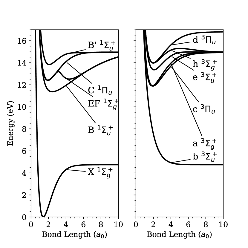
Figure 1: Potential energy curves for the ground state and the lower-lying excited states, relative to the ground state equilibrium energy. Data from Kolos1986, Staszewska1999, Staszewska2002, Wolniewicz1994 and Wolniewicz2003.

The R-matrix method relies on a balanced description of the target and scattering wavefunctions, $N$ and $N+1$ respectively [jt189]. Where $N$ is the number of electrons in the target. Molecular hydrogen is a two electron system. Therefore we have aimed to use the most comprehensive models available in each case. Full-CI is the hallmark of accuracy in electronic structure methods and it provides an exact solution to the Schrödinger equation within a given finite-sized one-electron basis set. This method is used with an augmented Dunning basis set, especially designed to describe Rydberg-type excitations in molecules, x-aug-cc-pVXZ [Dunning1989, Woon1994]. x-aug signifies that the basis set is doubly, triply, quadruply-augmented where x = d, t, q, etc. Triply augmented means that three additional, even-tempered basis functions are added for each angular symmetry available in the original cc-pVXZ set. Traditional Dunning basis sets, cc-pVXZ, are correlation consistent and hence provide a systematic way of approaching the complete basis set limit as the number X of zeta functions is increased. Preliminary work found that moving from a singly augmented basis set to a triply augmented basis set had a more profound effect on the target description than increasing the number of zeta functions i.e., pVXZ for X = D, T, Q, etc. For the R-matrix calculations, presented in this work, we found that t-aug-cc-pVTZ was the optimal choice (tAVTZ hereafter).

As mentioned previously, we are using Full-CI and the tAVTZ basis set. Therefore, our target model (in D_2h symmetry) can be expressed as $(19,9,9,4,19,9,9,4)^{2}$. Using this model we can solve the $N$-electron problem and calculate target state energies (on average, 400 configuration state functions are generated per molecular spin-space symmetry). Target state energies were calculated at the equilibrium geometry $R_{e}=1.40\ a_{0}$ to compare with accurate structure calculations of Kolos1986, Staszewska1999, Staszewska2002, Wolniewicz1994, Wolniewicz2003 and the MCCC calculations of Zammit2017a (see Table 1). Potential energy curves from the aforementioned references are also provided in Fig. 1.

For the excited states considered in this work, the R-matrix method produces more accurate target states than the spherical MCCC method. This is due to the difference in how the target is expanded in the two methods. MCCC uses single centre expansion, which performs worse for lower target states, however it quickly improves for the higher lying, Rydberg-like states. The R-matrix method however uses a linear combination of atom-centered GTOs. This generally performs better for the ground and low-lying excited states and in this work it performs well for all the states listed in Table 1.

Table 1: Absolute target energies, E (a.u.), at the equilibrium bond length $R_{e}=1.40\ a_{0}$ compared to accurate electronic structure calculations.

	E (a.u.)
state	Ref	RMf	MCCCg
$X\ ^{1}\Sigma_{g}^{+}$	-1.174a	-1.173	-1.162
$b\ ^{3}\Sigma_{u}^{+}$	-0.784b	-0.784	-0.770
$a\ ^{3}\Sigma_{g}^{+}$	-0.714b	-0.713	-0.710
$B\ ^{1}\Sigma_{u}^{+}$	-0.706c	-0.705	-0.697
$c\ ^{3}\Pi_{u}$	-0.707b	-0.706	-0.701
$EF\ ^{1}\Sigma_{g}^{+}$	-0.692d	-0.691	-0.687
$C\ ^{1}\Pi_{u}$	-0.689e	-0.688	-0.683
$e\ ^{3}\Sigma_{u}^{+}$	-0.644b	-0.643	-0.640
$h\ ^{3}\Sigma_{g}^{+}$	-0.630b	-0.630	-0.628
$d\ ^{3}\Pi_{u}$	-0.629b	-0.628	-0.626
$B^{\prime}\ {}^{1}\Sigma_{u}^{+}$	-0.629c	-0.628	-0.625

^aKolos1986; ^bStaszewska1999; ^cStaszewska2002; ^dWolniewicz1994; ^eWolniewicz2003; ^fThis work; ^gZammit2017a.

2.1.2 Scattering Model

In the R-matrix method the electronic density of the target must be contained within the R-matrix sphere, which is of radius $a$. Due to the extremely diffuse nature of our basis set we used a radius of $a=100\ a_{0}$. Usually an R-matrix sphere of this size would be impossible, as the continuum basis set required to fill the space would suffer from severe linear dependence. However, as mentioned previously, the new UKRMol+ codes allow the use of BTOs which are numerically stable regardless of the size of the R-matrix sphere. We found that, for molecular hydrogen, using a BTO only continuum basis not only removed linear dependence issues but it also gave a better description of the continuum. Details of the continuum basis can be found in Table 2.

Table 2: Continuum Basis Parameters for the continuum basis.

Property	Value
Number of B-Splines (per $l$)	75
B-spline Order	9
$l_{\mathrm{max}}$	6

To solve the scattering problem we are using a close-coupling expansion. This is necessary for describing exchange and polarisation effects in addition to modelling electronic excitation. To ensure balance between the $N+1$ and $N$-electron contributions in the close-coupling expansion we use a similar treatment in the $N+1$ electron system as we did for the target. We adopt two types of configuration state function (CSF) in the $N+1$ system. There are those where one electron occupies a continuum orbital, and those where all of the $N+1$ electrons occupy the target molecular orbitals. This amounts to;

$$(target)^{2}(continuum)^{1},$$

$$(target)^{3},$$

where $target$ stands for the complete set of target molecular orbitals. Note that in the first configuration step it is necessary to couple the target electrons to the appropriate symmetry, in order to facilitate the identification of the correct target states [jt180]. However, there are no constraints on the “$L^{2}$” configurations generated in the second step. Using this model we retain all the target states below 30 eV vertical excitation energy, which is 98 states. This generates an average of 65,000 CSFs per molecular symmetry.

Up to now differential cross-sections (DCS) obtained from R-matrix calculations were generated using the program POLYDCS [Sanna1998] which includes rotational excitation of the molecule but is limited to electronically elastic transitions. Therefore we have developed a new program for the calculation of DCS which includes only orientational averaging of the molecule but is applicable to electronically inelastic transitions and optionally employs the standard top-up procedure based on the first Born approximation for inelastic dipolar scattering. For details see A.

2.2 Molecular convergent close-coupling

The MCCC method is a momentum-space formulation of the close-coupling theory. The target spectrum is represented by a set of (pseudo)states generated by diagonalising the target electronic Hamiltonian in a basis of Sturmian (Laguerre) functions. For a suitable choice of basis the resulting states provide a sufficiently accurate representation of the low-lying discrete spectrum and a discretisation of the continuous spectrum, which allows the effects of coupling to ionisation channels to be modelled. Expanding the total scattering wave function in terms of the target pseudostates and performing a partial-wave expansion of the projectile wave function leads to a set of linear integral equations for the partial-wave $T$-matrix elements, which are solved using standard techniques. The strength of the MCCC method is the ability to perform calculations with very large close-coupling expansions, allowing for the explicit demonstration of convergence in the scattering quantities of interest with respect to the number of target states included in the calculations and the size of the projectile partial-wave expansion.

The MCCC method has been implemented for electron and positron scattering on diatomic molecules in both spherical and spheroidal coordinates. The spherical implementation is simpler and provides an adequate description of the molecular structure at the mean internuclear separation of the H₂ ground state. We have utilised the spherical MCCC method for detailed convergence studies and the calculation of elastic, excitation, ionisation, and grand-total cross-sections over a wide range of incident energies. Spheroidal coordinates are a more natural system for describing the electronic structure at larger $R$, where the target wave functions become more diffuse. We have utilised the spheroidal MCCC method to calculate vibrationally-resolved cross-sections for excitation of a number of low-lying states of H₂, including scattering on all bound vibrational levels of the ground electronic state [Scarlett19adndt]. This has allowed detailed studies to be performed for dissociation of H₂ in the ground and vibrationally-excited states [atoms7030075, TSSFZB18, Tapley18, Scarlett_diss2018], and vibrational excitation of the $X~{}^{1}\Sigma_{g}^{+}$ state via electronic excitation and radiative decay [Scarlett_2019]. For clarity of presentation, in the present paper we present only the spherical MCCC results. For details of the spheroidal MCCC method and comparisons of the spherical and spheroidal MCCC cross sections see posmolCCC19.

2.2.1 Target Model

The MCCC target structure is obtained using a CI calculation. The basis for the CI expansion consists of two-electron configurations formed by products $(n\ell,n^{\prime}\ell^{\prime})$ of one-electron Laguerre-based orbitals. To reduce the number of two-electron states generated, we allow one of the target electrons to occupy any one-electron orbital, while the other is restricted to the $1s$, $2s$, and $2p$ orbitals. The largest target structure calculation we have performed utilises a Laguerre basis of $N_{\ell}=17-\ell$ functions with $\ell\leq 3$, which generates a total of 491 states. To improve the accuracy of the $X~{}^{1}\Sigma_{g}^{+}$ and $b~{}^{3}\Sigma_{u}^{+}$ states, where the multicentre effects are strongest, we replace the $1s$ Laguerre function with an accurate H${}_{2}^{+}$ $1s\sigma_{g}$ state obtained via diagonalisation of the H${}_{2}^{+}$ Hamiltonian in a basis with $N_{\ell}=60-\ell$ functions for $\ell\leq 8$.

2.2.2 Scattering Models

Fixed-Nuclei (FN) MCCC calculations were performed at $R=1.448\ a_{0}$ using a number of scattering models, ranging from 9 to 491 states included in the close-coupling expansion. This allowed for a detailed investigation of convergence and the effects of including various reaction channels (see Zammit2017a for details). The MCCC results presented here were obtained from the 491-state model, which yielded convergent cross-sections for each of the transitions of interest. With regards to the partial-wave expansion of the projectile wave function, we have included angular momenta up to $L_{\mathrm{max}}=8$, and all total angular momentum projections up to ${M_{\mathrm{max}}=L_{\mathrm{max}}}$. To account for the contributions from higher partial waves we utilise an analytical Born subtraction (ABS) technique, which is equivalent to replacing the $L>L_{\mathrm{max}}$ cross-sections with their respective partial-wave Born cross-sections. We have found that the partial-wave expansion with $L_{\mathrm{max}}=8$ produces convergent integrated cross sections (ICS) for all transitions considered here when used in conjunction with the ABS technique. For dipole-allowed transitions, the partial-wave convergence of the DCS can be considerably slower than it is for the ICS. The method we have adopted to resolve this issue is discussed in Zammit2017a. For the $X~{}^{1}\Sigma_{g}^{+}\rightarrow b~{}^{3}\Sigma_{u}^{+}$ transition, adiabatic-nuclei calculations have been performed at low incident energies using a model consisting of 12 target states which yields convergent cross-sections for the $b~{}^{3}\Sigma_{u}^{+}$ state below approximately 15 eV. These calculations are described in Scarlett17b3.

2.3 Adiabatic-Nuclei Approximation

So far we have discussed FN calculations. However, in reality, the molecular geometry is not fixed and experiment effectively samples from a range of initial and final states. This will have an impact on both the integrated and differential cross-sections. This behaviour is most notable near threshold [jt229]. At higher scattering energies, away from the threshold, the two approximations converge as nuclear motion effects become less significant. We use the Adiabatic-Nuclei (AN) approach detailed in Lane1980 which has been recently demonstrated by Scarlett17b3 on molecular hydrogen. In this work we use the ground vibrational wavefunction to vibrationally average multiple FN calculations, carried out at a range of different nuclear geometries. Although, in general, this method can also be used to produce vibrationally resolved cross-sections.

Table 3: Absolute target energies, E (a.u.), and vertical excitation energies, $\Delta$E (eV), at the mean vibrational bond length $R_{0}=1.448\ a_{0}$. RM data are from UKRMol+ (this work) and MCCC from Zammit2017a.

	E (a.u.)			$\Delta$E (eV)
State	RM	MCCC		RM	MCCC
$X\ ^{1}\Sigma_{g}^{+}$	-1.172	-1.161		-	-
$b\ ^{3}\Sigma_{u}^{+}$	-0.796	-0.782		10.23	10.31
$a\ ^{3}\Sigma_{g}^{+}$	-0.718	-0.715		12.35	12.14
$B\ ^{1}\Sigma_{u}^{+}$	-0.712	-0.704		12.52	12.44
$c\ ^{3}\Pi_{u}$	-0.712	-0.707		12.52	12.35
$EF\ ^{1}\Sigma_{g}^{+}$	-0.697	-0.693		12.93	12.73
$C\ ^{1}\Pi_{u}$	-0.694	-0.693		13.02	12.73
$e\ ^{3}\Sigma_{u}^{+}$	-0.650	-0.647		14.21	13.99
$h\ ^{3}\Sigma_{g}^{+}$	-0.636	-0.634		14.60	14.34
$B^{\prime}\ {}^{1}\Sigma_{u}^{+}$	-0.635	-0.631		14.63	14.42
$d\ ^{3}\Pi_{u}$	-0.634	-0.632		14.65	14.39

3 Results

In this section, we present FN ICS and DCS for elastic and inelastic processes. For inelastic processes we consider the first ten electronic excited states. In the second section we use the adiabatic-nuclei approximation to introduce nuclear motion effects which are particularly important close to threshold. The FN R-matrix ICS and DCS data are provided as supplementary data.

The scattering calculations that follow were carried out at the mean vibrational bond length, $R_{0}=1.448\ a_{0}$, to provide the best comparison to experiment, within the FN approximation. Table 3 lists the target states and the vertical excitation energies obtained for both methods. Similarly, compared to Table 1, the R-matrix target energies are more accurate than the MCCC method, as they are lower in energy (note that both methods are variational). However, it should be noted that the absolute energy is of less significance for this work, and that the vertical excitation energies (relative to the ground state) are in good agreement.

3.1 Fixed-Nuclei Cross-Sections

We present ICS and DCS for the first ten target states (see Table 3); $X\ ^{1}\Sigma_{g}^{+}$, $b\ ^{3}\Sigma_{u}^{+}$, $a\ ^{3}\Sigma_{g}^{+}$, $B\ ^{1}\Sigma_{u}^{+}$, $c\ ^{3}\Pi_{u}$, $EF\ ^{1}\Sigma_{g}^{+}$, $C\ ^{1}\Pi_{u}$, $e\ ^{3}\Sigma_{u}^{+}$, $h\ ^{3}\Sigma_{g}^{+}$, $B^{\prime}\ {}^{1}\Sigma_{u}^{+}$ and $d\ ^{3}\Pi_{u}$. Where available, recommended cross-sections and experimental results are plotted against the two theoretical calculations.

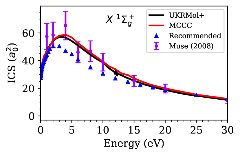
Figure 2: ICS for elastic collisions. Comparison of the UKRMol+ and MCCC calculations with the measurements of Muse2008 and recommended data of Yoon2008.

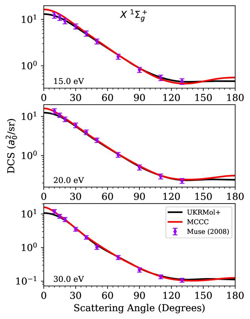
Figure 3: DCS for elastic collisions. Comparison of the UKRMol+ and MCCC calculations with the measurements of Muse2008.

3.1.1 Elastic Cross-Sections

The elastic ICS (Fig. 2) demonstrates good agreement between MCCC and R-matrix theory. The calculated data lie within the error bars of the experiment conducted by Muse2008. For the DCS (Fig. 3) at scattering angles exceeding 15^∘ the two theories essentially overlap. At energies greater than 15 eV the R-matrix calculations have a diminished forward peak and this is due to a lack of convergence of the partial wave expansion. Due to computational constraints $L_{\mathrm{max}}=6$ for the R-matrix calculations. This compares to $L_{\mathrm{max}}=8$ for the MCCC calculation, which also employs the ABS technique. Nevertheless, scattering angles close to $\theta=$ 0 or $\theta=$ 180 do not contribute as much to the ICS due to a $\sin\theta$ term in the integrand. Therefore, despite the differences in the DCSs the resulting ICSs are similar.

The recommended data of Yoon2008 for the ICS are noticeably lower than those obtained from the R-matrix and MCCC calculations (Fig. 2). Whilst they are within their specified margin of error ($\pm 20\%$) we believe that, due to the excellent agreement between both theories and experiment for the DCS (Fig. 3), the recommended data should be revised.

3.1.2 Triplet States

The first excited electronic state is $b\ ^{3}\Sigma_{u}^{+}$. For this state we have used a fine energy grid for both the MCCC and UKRMol+ calculations. This allows an accurate comparison of the two ICSs. In Fig. 4 prominent resonance structures are observed near 12 eV. Across the energy range considered the two calculations agree.

The current recommended cross-sections agree at low energy but from 15 eV to 20 eV they appear to overestimate the cross-section. The newer experiment from Zawadzki2018 is much closer to the two theories. The DCSs (Fig. 5) also agree closely with these experimental data. The R-matrix calculations are a little higher than the MCCC calculations for angles exceeding 135^∘ but, again, the affect on the ICS is insignificant.

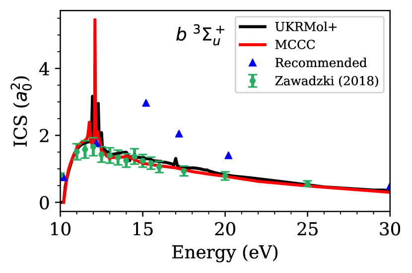
Figure 4: ICS for the $X\ ^{1}\Sigma_{g}^{+}\rightarrow b\ ^{3}\Sigma_{u}^{+}$ transition. Comparison of the UKRMol+ and MCCC calculations with the measurements of Zawadzki2018 and recommended data of Yoon2008.

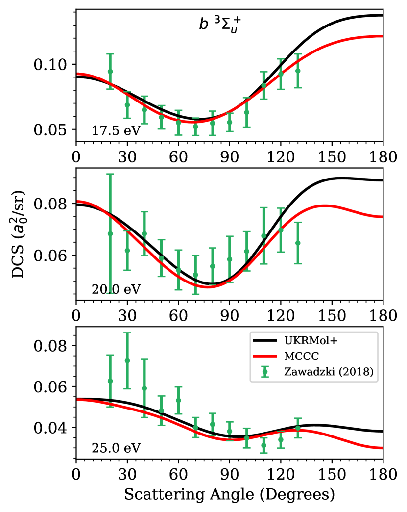
Figure 5: DCS for the $X\ ^{1}\Sigma_{g}^{+}\rightarrow b\ ^{3}\Sigma_{u}^{+}$ transition. Comparison of the UKRMol+ and MCCC calculations with the measurements of Zawadzki2018.

For higher excited states i.e., those energetically above $b\ ^{3}\Sigma_{u}^{+}$, MCCC results are presented on a coarser energy grid. Therefore, we can no longer compare the narrow resonant structures. The ICSs for states $a\ ^{3}\Sigma_{g}^{+}$, $c\ ^{3}\Pi_{u}$ and $e\ ^{3}\Sigma_{u}^{+}$ (Figs. 6, 8 and 10 respectively) have good agreement between the MCCC and R-matrix theories.

The recommended data points are based on the EELS (Electron Energy Loss Spectroscopy) experiment of Wrkich2002. The data points are sparse so it is hard to quantitatively compare against the two theory calculations. However, given agreement between the two theoretical calculations and more recent experiments, we believe that the recommended cross-sections should be revised for all of the triplet states considered so far.

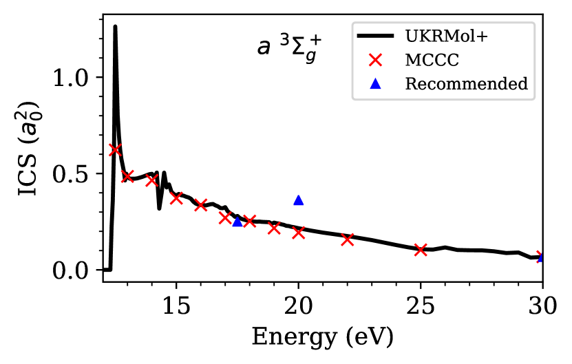
Figure 6: ICS for the $X\ ^{1}\Sigma_{g}^{+}\rightarrow a\ ^{3}\Sigma_{g}^{+}$ transition. Comparison of the UKRMol+ and MCCC calculations with the recommended data of Yoon2008.

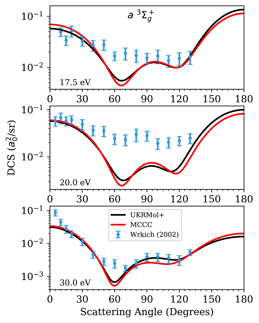
Figure 7: DCS for the $X\ ^{1}\Sigma_{g}^{+}\rightarrow a\ ^{3}\Sigma_{g}^{+}$ transition. Comparison of the UKRMol+ and MCCC calculations with the measurements of Wrkich2002.

The DCSs shed more light on the comparison. Fig. 7 shows the $a\ ^{3}\Sigma_{g}^{+}$ state. Agreement is best for 17.5 eV and 30 eV. The general shape is present at all three energies. That is, the cross-section dips around 60^∘ and 120^∘. However, for intermediate angles the magnitude of the DCS is higher (especially for 20 eV) than the theoretical calculations. EELS experiments are hard to conduct for excited states of H₂ because the states overlap in the spectra and the individual components have to be deconvoluted. Based on the difficulty of these type of experiments for highly-excited states we suggest that the calculations are more reliable.

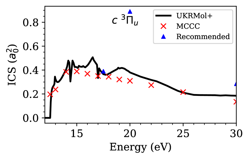
Figure 8: ICS for the $X\ ^{1}\Sigma_{g}^{+}\rightarrow c\ ^{3}\Pi_{u}$ transition. Comparison of the UKRMol+ and MCCC calculations with the recommended data of Yoon2008.

Figure 9: DCS for the $X\ ^{1}\Sigma_{g}^{+}\rightarrow c\ ^{3}\Pi_{u}$ transition. Comparison of the UKRMol+ and MCCC calculations with the measurements of Wrkich2002.

For the $c\ ^{3}\Pi_{u}$ state (Fig. 9) the situation is similar to the $a\ ^{3}\Sigma_{g}^{+}$ state. There is a slight downward slope towards higher scattering angles that is present in both the calculation and the experiment. However, the experimental DCS at 20 eV is approximately an order of magnitude higher.

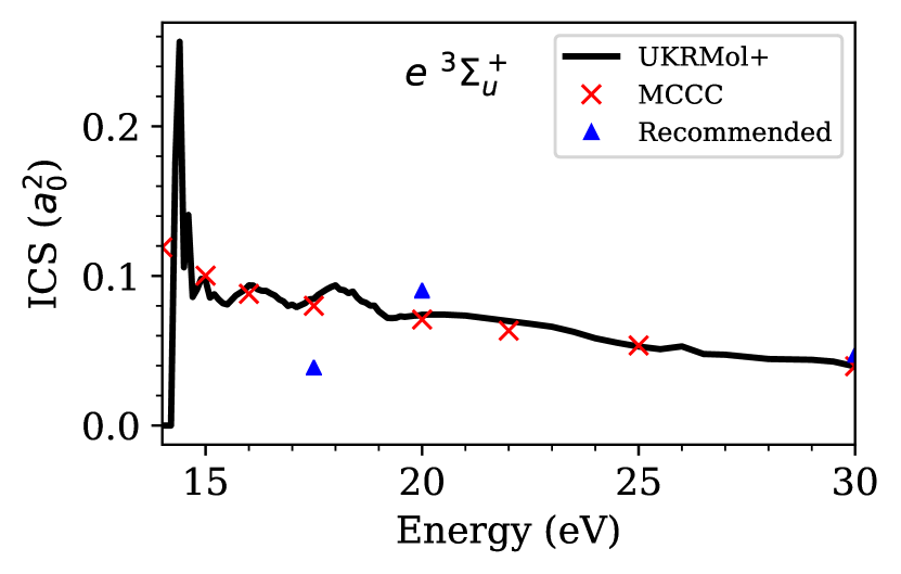
Figure 10: ICS for the $X\ ^{1}\Sigma_{g}^{+}\rightarrow e\ ^{3}\Sigma_{u}^{+}$ transition. Comparison of the UKRMol+ and MCCC calculations with the recommended data of Yoon2008.

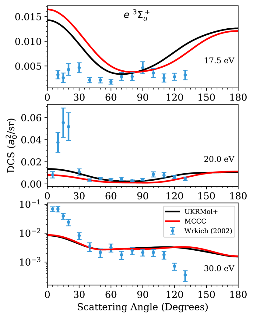
Figure 11: DCS for the $X\ ^{1}\Sigma_{g}^{+}\rightarrow e\ ^{3}\Sigma_{u}^{+}$ transition. Comparison of the UKRMol+ and MCCC calculations with the measurements of Wrkich2002.

For the $e\ ^{3}\Sigma_{u}^{+}$ state there is no qualitative agreement between theory and experiment. At all three energies (shown in Fig. 11) we have large discrepancies for low angle scattering i.e., below 30^∘. This is not too surprising though as low and high angle scattering is difficult to measure due to the physical constraints of the experimental setup. Therefore, we suspect that the low angle cross-sections measured by Wrkich2002, at 20 eV and 30 eV, are too high.

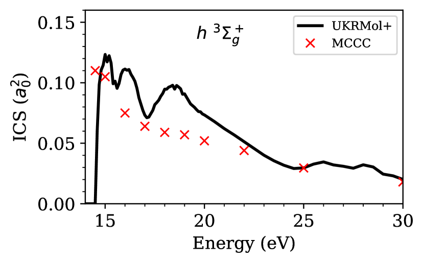
Figure 12: ICS for the $X\ ^{1}\Sigma_{g}^{+}\rightarrow h\ ^{3}\Sigma_{g}^{+}$ transition. Comparison of the UKRMol+ and MCCC calculations.

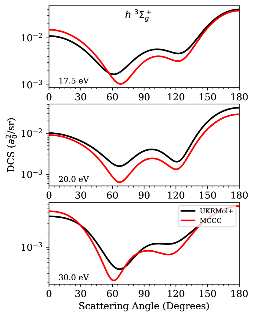
Figure 13: DCS for the $X\ ^{1}\Sigma_{g}^{+}\rightarrow h\ ^{3}\Sigma_{g}^{+}$ transition. Comparison of the UKRMol+ and MCCC calculations.

The ICSs for states $h\ ^{3}\Sigma_{g}^{+}$ and $d\ ^{3}\Pi_{u}$ (Figs. 12 and 14) show agreement between the two theories. However, the R-matrix calculation exhibits pronounced features around 16 eV and 19 eV. In the standard R-matrix approach used in this work, ionisation effects are not included. We include states above the ionisation threshold but we do not explicitly include pseudostates. To model ionisation pseudostates are required as implemented in the R-matrix with pseudostates (RMPS) method [Gorfinkiel2005]. As a result, the cross-section is overestimated above ionisation threshold. This behaviour was demonstrated previously in MCCC calculations when only the bound states were used [Zammit2017a]. In addition, weak transitions can also suffer from small oscillations, but the impact is reduced as the size of the close-coupling expansion increases. Therefore, the enhanced R-matrix cross-section is likely due to missing ionisation channels.

The R-matrix DCSs for state $h\ ^{3}\Sigma_{g}^{+}$ (Fig. 13) show broad agreement with the MCCC data. There are no recommended data for either the $h\ ^{3}\Sigma_{g}^{+}$ or $d\ ^{3}\Pi_{u}$ states. For the $d\ ^{3}\Pi_{u}$ state (Fig. 15) there are more significant differences between the two theories. As the target excitation increases, we typically expect less agreement between the two theories. Higher excited states tend to be less accurately described by the electronic structure calculations used in the R-matrix method.

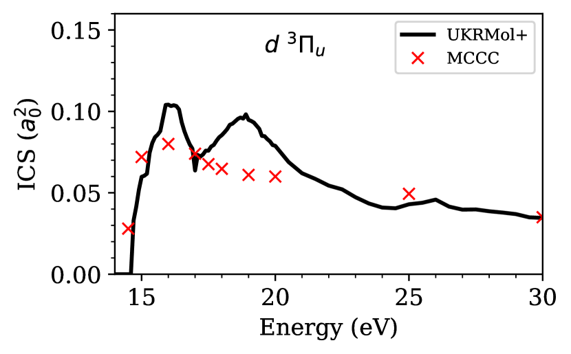
Figure 14: ICS for the $X\ ^{1}\Sigma_{g}^{+}\rightarrow d\ ^{3}\Pi_{u}$ transition. Comparison of the UKRMol+ and MCCC calculations.

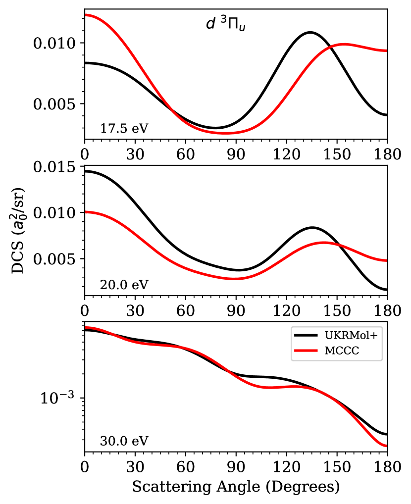
Figure 15: DCS for the $X\ ^{1}\Sigma_{g}^{+}\rightarrow d\ ^{3}\Pi_{u}$ transition. Comparison of the UKRMol+ and MCCC calculations.

3.1.3 Singlet States

Next we consider the singlet states. ICSs for three dipole-allowed states, $B\ ^{1}\Sigma_{u}^{+}$, $C\ ^{1}\Pi_{u}$ and $B^{\prime}\ {}^{1}\Sigma_{u}^{+}$, are shown in Figs. 16, 18 and 20 respectively. All three ICSs show excellent agreement between MCCC and R-matrix theory. Furthermore, agreement with the recommended data, which is available for the $B\ ^{1}\Sigma_{u}^{+}$ and $C\ ^{1}\Pi_{u}$ states, is extremely good at the energies considered here. Contrary to the previous EELS experimental data, these recommended data were measured from the optical emission of the electron impact electronically excited B and C states [Liu1998].

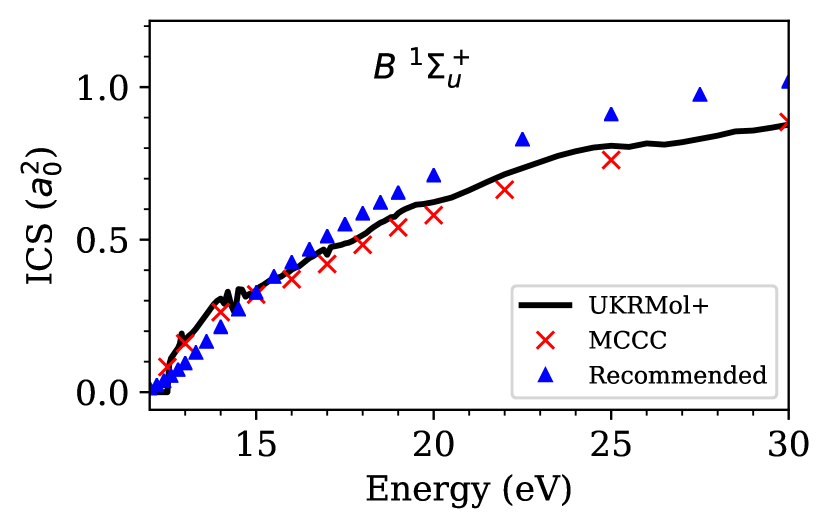
Figure 16: ICS for the $X\ ^{1}\Sigma_{g}^{+}\rightarrow B\ ^{1}\Sigma_{u}^{+}$ transition. Comparison of the UKRMol+ and MCCC calculations with the recommended data of Yoon2008.

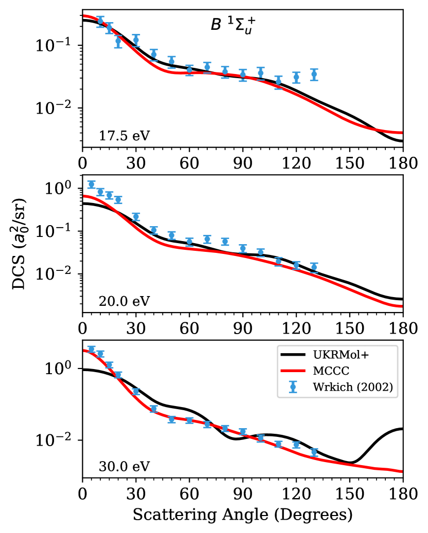
Figure 17: DCS for the $X\ ^{1}\Sigma_{g}^{+}\rightarrow B\ ^{1}\Sigma_{u}^{+}$ transition. Comparison of the UKRMol+ and MCCC calculations with the measurements of Wrkich2002.

DCSs could not be determined in the emission experiments of Liu1998. However, Wrkich2002 produced a set of EELS DCS which have been plotted in Figs. 17 and 19. For the $B\ ^{1}\Sigma_{u}^{+}$ state the agreement with experiment is good. At 30 eV however the R-matrix calculation displays oscillations that are not present in the MCCC Calculation. This is due to a lack of convergence in the partial-wave expansion. Typically a Born correction would be applied to dipole allowed transitions. However, in the present work this has not been possible. The Born top-up requires a sufficiently converged cross-section, up to some intermediate number of partial waves, $\bar{L}_{\mathrm{max}}$. For MCCC this is found to be $\bar{L}_{\mathrm{max}}=25$, or more, depending on the scattering energy [Zammit2017a]. A similar approach was attempted for the R-matrix calculation. Although this was not tractable given currently available software and computational power (see A).

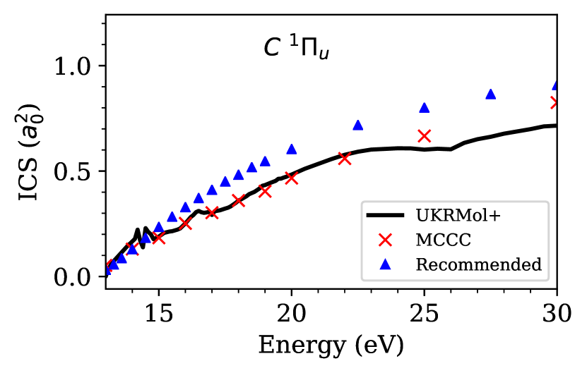
Figure 18: ICS for the $X\ ^{1}\Sigma_{g}^{+}\rightarrow C\ ^{1}\Pi_{u}$ transition. Comparison of the UKRMol+ and MCCC calculations with the recommended data of Yoon2008.

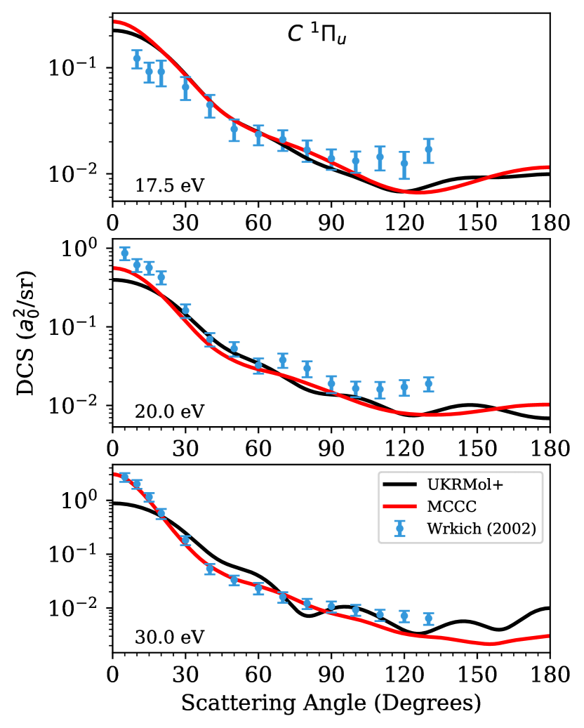
Figure 19: DCS for the $X\ ^{1}\Sigma_{g}^{+}\rightarrow C\ ^{1}\Pi_{u}$ transition. Comparison of the UKRMol+ and MCCC calculations with the measurements of Wrkich2002.

Similarly, the oscillations observed for the $B\ ^{1}\Sigma_{u}^{+}$ state at higher energies are also observed in states $C\ ^{1}\Pi_{u}$ and $B^{\prime}\ {}^{1}\Sigma_{u}^{+}$ (Figs. 19 and 21). Furthermore, in all of the singlet state DCSs, Figs. 17, 19, 21 and 22, the R-matrix calculation has a lower forward peak. This is attributed, as in the elastic scattering case, to a lack of convergence in the number of partial waves used. Regardless, forward and backward scattering only make a small contribution to the total ICS. Therefore the differences caused by the oscillatory behaviour and lower forward peak are lost upon integration. This highlights the importance of using DCSs as a stringent test of theories. Two theories may produce the same ICS but have different angular profiles.

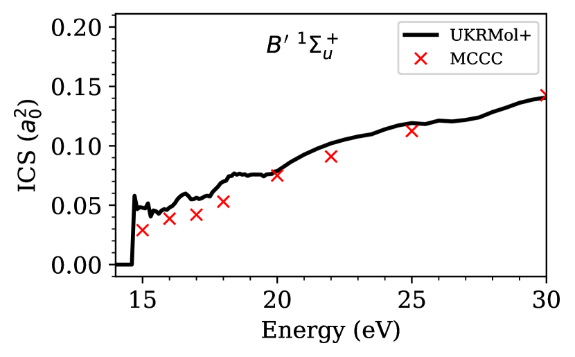
Figure 20: ICS for the $X\ ^{1}\Sigma_{g}^{+}\rightarrow B^{\prime}\ {}^{1}\Sigma_{u}^{+}$ transition. Comparison of the UKRMol+ and MCCC calculations.

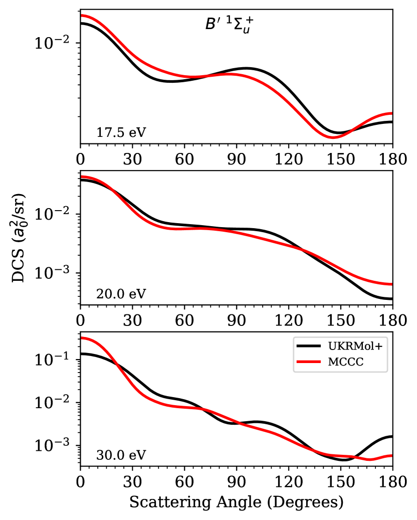
Figure 21: DCS for the $X\ ^{1}\Sigma_{g}^{+}\rightarrow B^{\prime}\ {}^{1}\Sigma_{u}^{+}$ transition. Comparison of the UKRMol+ and MCCC calculations.

In contrast to the dipole-allowed singlet states, the forbidden $EF\ ^{1}\Sigma_{g}^{+}$ state DCS (Fig. 22) is not as sensitive to higher partial-waves. Agreement between the two theories is good. The agreement between theory and experiment is acceptable, except for the scattering angles from 60^∘ to 100^∘ at 20 eV where the experiment gives a larger cross-section, which could be due to the analysis of the measured EELS.

Comparing the ICS (Fig. 23) between the two theories, the R-matrix calculation is consistently above the MCCC data. Again, this is due to the absence of ionisation channels in the R-matrix close-coupling expansion that leads to an overestimated cross-section.

The recommended data are based on an emission experiment carried out by Liu2003. Whilst the $EF\ ^{1}\Sigma_{g}^{+}$ state is dipole-forbidden, the cross-section can be inferred using a combination of theoretical and experimental considerations. There is a difference in threshold for experiment, which occurs near 15 eV as opposed to 13 eV for the FN MCCC and R-matrix calculations. However the magnitude and qualitative shape agree with theory.

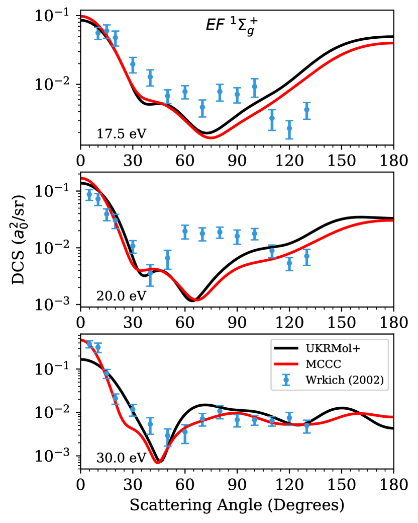
Figure 22: DCS for the $X\ ^{1}\Sigma_{g}^{+}\rightarrow EF\ ^{1}\Sigma_{g}^{+}$ transition. Comparison of the UKRMol+ and MCCC calculations with the measurements of Wrkich2002.

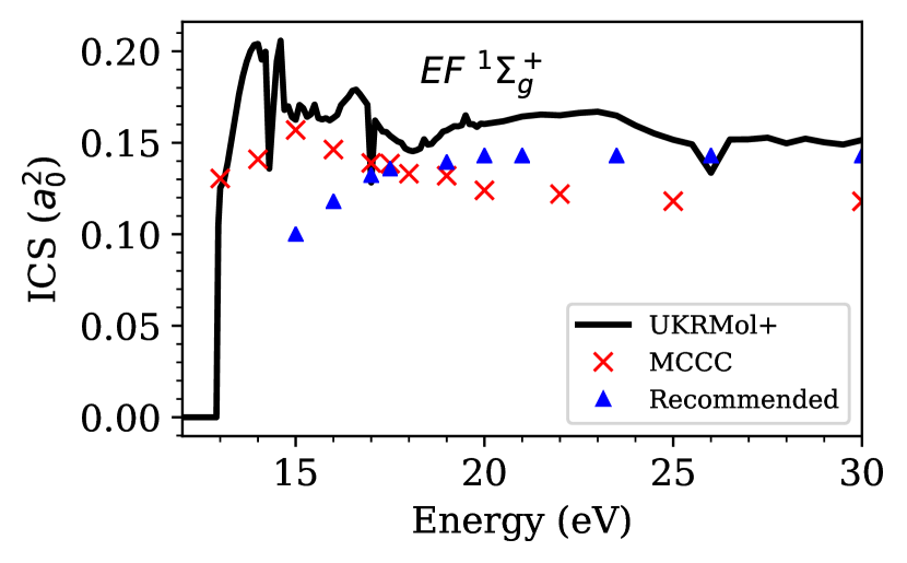
Figure 23: ICS for the $X\ ^{1}\Sigma_{g}^{+}\rightarrow EF\ ^{1}\Sigma_{g}^{+}$ transition. Comparison of the UKRMol+ and MCCC calculations with the recommended data of Yoon2008.

3.2 Adiabatic-Nuclei Cross-Sections

In this section we make use of the AN approximation described previously. In Fig. 24 both FN (dot-dashed line) and AN calculations (solid line) are shown side-by-side for electronic excitation to the first excited state ($X\ ^{1}\Sigma_{g}^{+}\rightarrow b\ ^{3}\Sigma_{u}^{+}$). For both the MCCC (red) and UKRMol+ (black) calculations we can see two main differences. The first is that resonant structures are washed-out and the second is that the sharp turn-on near the vertical excitation threshold (10 eV) is smoothed into a ramp. This is due to the vibrational averaging over different molecular geometries. The threshold for the $X\ ^{1}\Sigma_{g}^{+}\rightarrow b\ ^{3}\Sigma_{u}^{+}$ transition is essentially the vertical excitation energy. For some geometries this will be lower than 10 eV and for others will be greater. The average is weighted by the square of the ground vibrational wavefunction, which means the largest contributions occur at the maximum of the wavefunction i.e., about R₀. This is why the FN calculation at $R=R_{0}$ and the AN calculation are broadly similar. Adiabatic effects have consequences for near-threshold electron impact dissociation of H₂ [jt229].

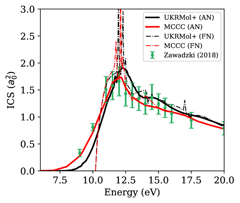
Figure 24: Integrated cross-section for the $X\ ^{1}\Sigma_{g}^{+}\rightarrow b\ ^{3}\Sigma_{u}^{+}$ transition using the AN approximation. (black) UKRMol+, (red) MCCC, (green dots) experiment from Zawadzki2018.

The AN approximation requires FN calculations to be performed across a grid of different internuclear bond separations. For the R-matrix calculations, a grid size of $\Delta R=0.05$ a.u. was used for $0.95<R<1.95$ a.u., with a finer grid of $\Delta R=0.01$ a.u. used in the region closer to the mean vibrational bond length, $1.35<R<1.55$ a.u. Due to the large number of FN calculations required it was not possible to use the full model described previously. Therefore a smaller model was used which featured a singly augmented aug-cc-pVTZ basis set and an R-matrix radius $a=25$ a.u. The smaller radius allowed the continuum representation to be simplified to 22 BTOs per angular momentum symmetry with $L_{\mathrm{max}}=4$ without sacrificing completeness. As before, all of the target states below 30 eV were included which led to a 59-state model. This model works well for the first excited state but due to the simplified target description it cannot represent higher-excited states.

4 Conclusion

In this paper we demonstrate good agreement with recent experimental data [Muse2008, Zawadzki2018], validated by two independent theories. The agreement with the recommended ICS data [Yoon2008] and older experimental data [Wrkich2002] is worse, predominantly for the triplet states but we believe this is due to the difficulties associated with the underlying experiments. That is, it is difficult for experiments to separate the overlapping contributions coming from different triplet excited states and therefore the error margin is larger for these types of experiment. Any other significant differences between the two theories and experiments are well understood.

This is the first time the CCC and R-matrix theories have been verified for a molecular target. This work presents one of the largest molecular R-matrix calculations to date. Many novel features have been exploited for the first time: a triply-augmented target basis set, a box size of 100 a.u. and the first B-spline only continuum for a molecular target. This shows that both MCCC and R-matrix method can be used to perform large-scale, high-accuracy close-coupling calculations.

We have compared both fixed-nuclei and adiabatic-nuclei cross-sections obtained using the R-matrix and MCCC methods. For FN calculations, dipole-forbidden states generally show better agreement in the DCSs. Dipole-forbidden states do not require a born top-up and generally converge quicker for the same number of partial waves, compared to dipole allowed transitions [Zammit2017a]. For the dipole-allowed states the R-matrix calculations show oscillatory behaviour but this could be eliminated by using a higher cutoff in the number of partial-waves. However, this is currently not tractable given currently available hardware and software.

All of the ICSs show good agreement between the two theories with the exclusion of weak transitions that are more sensitive to the absence of ionisation channels in the R-matrix calculations, leading to slightly enhanced cross-sections. The AN ICS for the first excited state shows excellent agreement between the two theories and the recent experimental data.

There are several directions for future work. Firstly, it would be interesting to compare the effect of target model used in the MCCC calculations i.e., spherical versus spheroidal. Preliminary results for the $EF\ ^{1}\Sigma_{g}^{+}$ state suggest that the use of a spheroidal model could improve the agreement between both theories.

Secondly, in order to accurately describe ionisation effects in the R-matrix method we would need to employ the RMPS method. Whilst the RMPS method is implemented in UKRMol+ the calculations for this system are currently too expensive.

Additionally, for the R-matrix calculations presented in this work we have not been able to carry out systematic, quantitative analysis of the uncertainties. This is a common problem across the field for theoretical calculations [jt642]. For future work, we seek a tractable approach that is capable of providing uncertainties for our calculated data.

Finally, a general approach for handling Born top-ups, similar to the ABS method used in MCCC calculations would be desirable for the UKRMol+ calculations in order to reach convergence where larger numbers of partial-waves are required (as discussed in A).

References

Appendix A Including Higher Partial Waves

To include higher partial waves, specifically for dipole-allowed transitions, we require a top-up procedure. In R-matrix calculations this is done using an approach suggested by Norcross1982. The MCCC uses an equivalent method described in [Zammit2017]. For a DCS the top up procedure is given by

$$\frac{d\sigma}{d\Omega}= \left(\frac{d\sigma}{d\Omega}\right)_{Born}+$$ (1)

$$\sum_{\lambda=0}^{\lambda_{max}}(A_{\lambda}-A_{\lambda}^{Born})P_{\lambda}(\cos\theta),$$

where the first term on the right hand side is the DCS calculated for inelastic dipolar scattering in the first Born approximation and the second term includes the contribution of the lower partial waves $A_{\lambda}$ calculated with close-coupling and subtraction of the corresponding Born partial waves $A_{\lambda}^{Born}$. Only orientational averaging of the molecule is taken into account. This approach was used in previous R-matrix calculations for inelastic collisions, but only for ICSs [jt256, jt429, Masin2012], which tend to converge quicker than DCSs. Recently, jtCO employed the Born correction described above for the electronically inelastic DCS of CO. This method, however, requires a sufficiently high partial wave cutoff, $L_{\mathrm{max}}$. At lower partial waves the analytic Born method is less accurate and tends to overestimate the cross-section, leading to unphysical negative cross-sections.

Born corrections have been successfully applied to DCSs for elastic collisions, see e.g., jt464 and Masin2012. However, these cross-sections are usually an order of magnitude larger than those for dipole-allowed inelastic transitions. Hence, they are less susceptible to the oscillatory behaviour seen in inelastic DCSs.

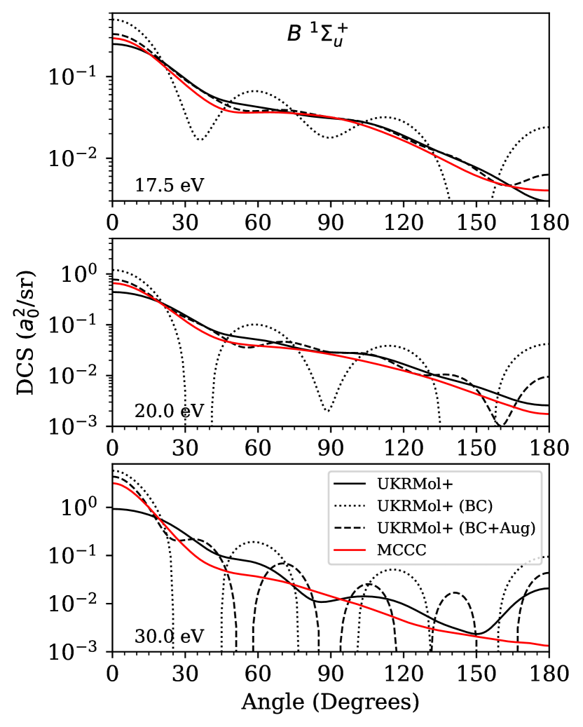
Figure 25: DCS for the $B\ ^{1}\Sigma_{u}^{+}$ state calculated using the R-matrix method, with $L_{\mathrm{max}}=6$ (black) and the MCCC method (red). The Born top-up was applied to the original calculation before (dotted) and after (dashed) the T-matrix elements were augmented with a cheaper $L_{\mathrm{max}}=10$ calculation.

Figure 25 shows the DCS for the dipole-allowed $B\ ^{1}\Sigma_{u}^{+}$ state. In solid black we have the original R-matrix calculation without the Born correction. If we apply the Born correction to the DCS we obtain the dotted line. At 17.5 eV, the Born corrected DCS displays unphysical behaviour around 150^∘ where it becomes negative. The situation worsens for higher energies. This is due to an incomplete convergence of the partial-wave Born contribution $\sum_{\lambda}A_{\lambda}^{Born}P_{\lambda}(\cos\theta)$.

To resolve this issue, the MCCC approach [Zammit2017a] has been to run a smaller-sized calculation but with a higher cutoff e.g., $\bar{L}_{\mathrm{max}}=25$. The results of this calculation are then used to augment the T-matrices of the more expensive calculation. This allows the DCS contributions from higher partial waves to be calculated with the more accurate MCCC theory before including the additional contributions from the Born procedure.

A similar approach has been adopted in the R-matrix calculations, however $\bar{L}_{\mathrm{max}}=25$ is currently not computationally feasible with the UKRMol+ codes. Calculations using a smaller model, but with $\bar{L}_{\mathrm{max}}=10$, have been computed and these were used to augment the T-matrices of the accurate R-matrix calculation with $L_{\mathrm{max}}=6$. When augmenting the T-matrix elements, care must be taken to phase-match the two calculations. This can be achieved by comparing the transition dipole moments of the target states involved in each transition.

The result of augmenting the T-matrices and applying the Born correction is shown as the dashed line in Fig. 25. For the lowest scattering energy shown, 17.5 eV, the oscillatory behaviour is greatly reduced and the Born correction improves the quality of agreement between the MCCC and R-matrix calculations. At 20 eV Born-corrected DCS is improved but it still shows oscillatory behaviour that is characteristic of a lack of convergence. At 30 eV, even with the augmented T-matrix elements the DCS remains oscillatory when the Born correction is applied.

In theory, an approach similar to the MCCC method can be developed for the R-matrix calculations but there are two factors that currently inhibit further improvement. The first is that the target states from cheaper calculations need to be shifted to the more accurate values from the expensive calculation. For the R-matrix calculations, presented in this work, the energies were shifted in the outer-region. This is not ideal and instead we need to implement the energy shift in the $N+1$ scattering calculation, similar to the approach used by jt208. Secondly, the outer-region quickly dominates the computational resources required, both physical RAM and CPU-time, as a large number of channels are generated for higher partial waves. Furthermore a sophisticated approach would need to be implemented in the outer-region to reduce the number of states included in the calculation.

As an alternative approach, we also attempted to top-up the DCS using a more basic method (not shown). We ran two cheaper calculations with small basis sets using $L_{\mathrm{max}}=6$ and $L_{\mathrm{max}}=10$. We took the difference between the two DCSs and used this to top-up the expensive calculation. This approach does help to capture the forward peak scattering but it was too susceptible to unphysical negative cross-sections when the differences between the cheap calculations became negative. This method behaved particularly poorly in regions where the cross-section was small.

In summary, we believe the MCCC approach to the Born top-up is the most sensible way forward, however there is still work to be done before it can be implemented in R-matrix calculations.

References

- [1] \harvarditemAnzai et al.2012Anzai2012 Anzai K, Kato H, Hoshino M, Tanaka H, Itikawa Y, Campbell L, Brunger M J, Buckman S J, Cho H, Blanco F, Garcia G, Limão-Vieira P \harvardand Ingólfsson O 2012 Eur. Phys. J. D 66, 36.
- [2] \harvarditemBaluja et al.2000jt256 Baluja K L, Mason N J, Morgan L A \harvardand Tennyson J 2000 J. Phys. B: At. Mol. Opt. Phys. 33, L677–L684.
- [3] \harvarditemBaluja et al.1985jt38 Baluja K L, Noble C J \harvardand Tennyson J 1985 J. Phys. B: At. Mol. Phys. 18, L851–L855.
- [4] \harvarditemBartschat et al.1996Bartschat1996 Bartschat K, Bray I, Burke P G \harvardand Scott M P 1996 J. Phys. B At. Mol. Opt. Phys 29, 5493–5503.
- [5] \harvarditemBartschat et al.2010Bartschat2010 Bartschat K, Kheifets A S, Fursa D V \harvardand Bray I 2010 J. Phys. B At. Mol. Opt. Phys. 43, 165205.
- [6] \harvarditemBranchett et al.1990Branchett1990a Branchett S E, Tennyson J \harvardand Morgan L A 1990 J. Phys. B At. Mol. Opt. Phys. 23, 4625–4639.
- [7] \harvarditemBranchett et al.1991Branchett1991 Branchett S E, Tennyson J \harvardand Morgan L A 1991 J. Phys. B At. Mol. Opt. Phys. 24, 3479–3490.
- [8] \harvarditemChung et al.2016jt642 Chung H K, Braams B J, Bartschat K, Császár A G, Drake G W F, Kirchner T, Kokoouline V \harvardand Tennyson J 2016 J. Phys. D: Appl. Phys. 49(36), 363002.
- [9] \harvarditemDarby-Lewis et al.2017Darby-Lewis2017 Darby-Lewis D, Mašín Z \harvardand Tennyson J 2017 J. Phys. B At. Mol. Opt. Phys. 50, 175201.
- [10] \harvarditemDunning1989Dunning1989 Dunning T H 1989 J. Chem. Phys. 90, 1007–1023.
- [11] \harvarditemGorfinkiel \harvardand Tennyson2005Gorfinkiel2005 Gorfinkiel J D \harvardand Tennyson J 2005 J. Phys. B At. Mol. Opt. Phys. 38, 1607–1622.
- [12] \harvarditemHargreaves et al.2017Hargreaves2017 Hargreaves L R, Bhari S, Adjari B, Liu X, Laher R, Zammit M C, Savage J S, Fursa D V, Bray I \harvardand Khakoo M A 2017 J. Phys. B At. Mol. Opt. Phys. 50, 225203.
- [13] \harvarditemKaur et al.2008jt429 Kaur S, Baluja K L \harvardand Tennyson J 2008 Phys. Rev. A 77, 032718.
- [14] \harvarditemKolos \harvardand Szalewicz1986Kolos1986 Kolos W \harvardand Szalewicz K 1986 J. Chem. Phys. 84, 3278.
- [15] \harvarditemLane1980Lane1980 Lane N F 1980 Rev. Mod. Phys. 52, 29–119.
- [16] \harvarditemLange et al.2006Lange2006 Lange M, Matsumoto J, Lower J, Buckman S, Zatsarinny O, Bartschat K, Bray I \harvardand Fursa D V 2006 J. Phys. B At. Mol. Opt. Phys. 39, 4179–4190.
- [17] \harvarditemLima et al.1985Lima1985 Lima M A P, Gibson T L, Huo W M \harvardand McKoy V 1985 J. Phys. B At. Mol. Phys. 18, 865–870.
- [18] \harvarditemLiu et al.2003Liu2003 Liu X, Shemansky D E, Abgrall H, Roueff E, Ahmed S M \harvardand Ajello J M 2003 J. Phys. B At. Mol. Opt. Phys. 36, 173–196.
- [19] \harvarditemLiu et al.1998Liu1998 Liu X, Shemansky D E, Ahmed S M, James G K \harvardand Ajello J M 1998 J. Geophys. Res. Sp. Phys. 103, 26739–26758.
- [20] \harvarditemMašín et al.2012Masin2012 Mašín Z, Gorfinkiel J D, Jones D B, Bellm S M \harvardand Brunger M J 2012 J. Chem. Phys. 136, 144310.
- [21] \harvarditemMašín et al.2020jt772 Mašín Z, Benda J, Gorfinkiel J D, Harvey A G \harvardand Tennyson J 2020 Comput. Phys. Commun. 249, 107092.
- [22] \harvarditemMuse et al.2008Muse2008 Muse J, Silva H, Lopes M C \harvardand Khakoo M A 2008 J. Phys. B At. Mol. Opt. Phys. 41, 095203.
- [23] \harvarditemNorcross \harvardand Padial1982Norcross1982 Norcross D W \harvardand Padial N T 1982 Phys. Rev. A 25, 226–238.
- [24] \harvarditemPitchford et al.2017jt647 Pitchford L C, Alves L L, Bartschat K, Biagi S F, Bordage M C, Bray I, Brion C E, Brunger M J, Campbell L, Chachereau A, Chaudhury B, Christophorou L G, Carbone E, Dyatko N A, Franck C M, Fursa D V, Gangwar R K, Guerra V, Haefliger P, Hagelaar G J M, Hoesl A, Itikawa Y, Kochetov I V, McEachran R P, Morgan W L, Napartovich A P, Puech V, Rabie M, Sharma L, Srivastava R, Stauffer A D, Tennyson J, de Urquijo J, van Dijk J, Viehland L A, Zammit M C, Zatsarinny O \harvardand Pancheshnyi S 2017 Plasma Proc. Polymers 14, 1600098.
- [25] \harvarditemRegeta et al.2016Regeta2016 Regeta K, Allan M, Mašín Z \harvardand Gorfinkiel J D 2016 J. Chem. Phys. 144, 24302.
- [26] \harvarditemSanna \harvardand Gianturco1998Sanna1998 Sanna N \harvardand Gianturco F 1998 Comput. Phys. Commun. 114, 142–167.
- [27] \harvarditemScarlett et al.2020, submittedScarlett19adndt Scarlett L H, Fursa D V, Zammit M C, Bray I, Ralchenko Yu \harvardand Davie K 2020, submitted Atom. Data Nucl. Data Tables .
- [28] \harvarditemScarlett et al.2020, acceptedposmolCCC19 Scarlett L H, Savage J S, Fursa D V, Bray I \harvardand Zammit M C 2020, accepted Eur. Phys. J. D .
- [29] \harvarditemScarlett, Savage, Fursa, Zammit \harvardand Bray2019atoms7030075 Scarlett L H, Savage J S, Fursa D V, Zammit M C \harvardand Bray I 2019 Atoms 7(3).
- [30] \harvarditemScarlett et al.2017Scarlett17b3 Scarlett L H, Tapley J K, Fursa D V, Zammit M C, Savage J S \harvardand Bray I 2017 Phys. Rev. A 96(6), 062708.
- [31] \harvarditemScarlett et al.2018Scarlett_diss2018 Scarlett L H, Tapley J K, Fursa D V, Zammit M C, Savage J S \harvardand Bray I 2018 Eur. Phys. J. D 72(2), 34.
- [32] \harvarditemScarlett, Tapley, Savage, Fursa, Zammit \harvardand Bray2019Scarlett_2019 Scarlett L H, Tapley J K, Savage J S, Fursa D V, Zammit M C \harvardand Bray I 2019 Plasma Sources Science and Technology 28(2), 025004.
- [33] \harvarditemSchneider \harvardand Collins1985Schneider1985 Schneider B I \harvardand Collins L A 1985 J. Phys. B At. Mol. Phys. 18, L857–L863.
- [34] \harvarditemStaszewska \harvardand Wolniewicz1999Staszewska1999 Staszewska G \harvardand Wolniewicz L 1999 J. Mol. Spectrosc. 198, 416–420.
- [35] \harvarditemStaszewska \harvardand Wolniewicz2002Staszewska2002 Staszewska G \harvardand Wolniewicz L 2002 J. Mol. Spectrosc. 212, 208–212.
- [36] \harvarditemStibbe \harvardand Tennyson1997jt208 Stibbe D T \harvardand Tennyson J 1997 Phys. Rev. Lett. 79, 4116–4119.
- [37] \harvarditemStibbe \harvardand Tennyson1998jt229 Stibbe D T \harvardand Tennyson J 1998 New J. Phys 1, 2.
- [38] \harvarditemTapley, Scarlett, Savage, Fursa, Zammit \harvardand Bray2018TSSFZB18 Tapley J K, Scarlett L H, Savage J S, Fursa D V, Zammit M C \harvardand Bray I 2018 Phys. Rev. A 98, 032701.
- [39] \harvarditemTapley, Scarlett, Savage, Zammit, Fursa \harvardand Bray2018Tapley18 Tapley J K, Scarlett L H, Savage J S, Zammit M C, Fursa D V \harvardand Bray I 2018 Journal of Physics B: Atomic, Molecular and Optical Physics 51(14), 144007.
- [40] \harvarditemTawara et al.1990Tawara1990 Tawara H, Itikawa Y, Nishimura H \harvardand Yoshino M 1990 J. Phys. Chem. Ref. Data 19, 617–636.
- [41] \harvarditemTennyson1996ajt180 Tennyson J 1996a J. Phys. B: At. Mol. Opt. Phys. 29, 1817–1828.
- [42] \harvarditemTennyson1996bjt189 Tennyson J 1996b J. Phys. B: At. Mol. Opt. Phys. 29, 6185–6201.
- [43] \harvarditemTennyson2010jt474 Tennyson J 2010 Phys. Rep. 491, 29–76.
- [44] \harvarditemWolniewicz \harvardand Dressler1994Wolniewicz1994 Wolniewicz L \harvardand Dressler K 1994 J. Chem. Phys. 100, 444–451.
- [45] \harvarditemWolniewicz \harvardand Staszewska2003Wolniewicz2003 Wolniewicz L \harvardand Staszewska G 2003 J. Mol. Spectrosc. 220, 45–51.
- [46] \harvarditemWoon \harvardand Dunning1994Woon1994 Woon D E \harvardand Dunning T H 1994 J. Chem. Phys. 100, 2975–2988.
- [47] \harvarditemWrkich et al.2002Wrkich2002 Wrkich J, Mathews D, Kanik I, Trajmar S \harvardand Khakoo M A 2002 J. Phys. B At. Mol. Opt. Phys. 35, 4695–4709.
- [48] \harvarditemYoon et al.2008Yoon2008 Yoon J S, Song M Y, Han J M, Hwang S H, Chang W S, Lee B \harvardand Itikawa Y 2008 J. Phys. Chem. Ref. Data 37, 913.
- [49] \harvarditemZammit, Fursa, Savage \harvardand Bray2017Zammit2017 Zammit M C, Fursa D V, Savage J S \harvardand Bray I 2017 J. Phys. B At. Mol. Opt. Phys. 50, 123001.
- [50] \harvarditemZammit, Savage, Fursa \harvardand Bray2017Zammit2017a Zammit M C, Savage J S, Fursa D V \harvardand Bray I 2017 Phys. Rev. A 95, 022708.
- [51] \harvarditemZawadzki et al.2020jtCO Zawadzki M, Khakoo M A, Voorneman L, Ratkovic L, Mašín Z, Houfek K, Dora A \harvardand Tennyson J 2020. submitted.
- [52] \harvarditemZawadzki et al.2018Zawadzki2018 Zawadzki M, Wright R, Dolmat G, Martin M F, Diaz B, Hargreaves L, Coleman D, Fursa D V, Zammit M C, Scarlett L H, Tapley J K, Savage J S, Bray I \harvardand Khakoo M A 2018 Phys. Rev. A 98, 062704.
- [53] \harvarditemZhang et al.2009jt464 Zhang R, Faure A \harvardand Tennyson J 2009 Phys. Scr. 80, 015301.
- [54]