Double Happiness: Enhancing the Coupled
Gains of L-lag Coupling via Control Variates
Radu V. Craiu and Xiao-Li Meng
University of Toronto and Harvard University
Abstract: The recently proposed L-lag coupling for unbiased Markov chain Monte Carlo (MCMC) calls for a joint celebration by MCMC practitioners and theoreticians. For practitioners, it circumvents the thorny issue of deciding the burn-in period or when to terminate an MCMC sampling process, and opens the door for safe parallel implementation. For theoreticians, it provides a powerful tool to establish elegant and easily estimable bounds on the exact error of an MCMC approximation at any finite number of iterates. A serendipitous observation about the bias-correcting term leads us to introduce naturally available control variates into the L-lag coupling estimators. In turn, this extension enhances the coupled gains of L-lag coupling, because it results in more efficient unbiased estimators, as well as a better bound on the total variation error of MCMC iterations, albeit the gains diminish as L increases. Specifically, the new upper bound is theoretically guaranteed to never exceed the one given previously. We also argue that L-lag coupling represents a coupling for the future, breaking from the coupling-from-the-past type of perfect sampling, by reducing the generally unachievable requirement of being perfect to one of being unbiased, a worthwhile trade-off for ease of implementation in most practical situations. The theoretical analysis is supported by numerical experiments that show tighter bounds and a gain in efficiency when control variates are introduced.
Key words and phrases: Coupling from the Past, Maximum coupling, Median absolute deviation, Parallel implementation, Total variation distance, Unbiased MCMC.
1 If Being Perfect Is Impossible, Let’s Try Being Unbiased
1.1 Perfect Coupling – Too Much To Hope For?
We thank Pierre Jacob and his team for a series of articles (e.g., Jacob et al., 2020, 2019; Heng and Jacob, 2019; Biswas et al., 2019) that revitalized our experience (e.g., Murdoch and Meng, 2001; Meng, 2000; Craiu and Meng, 2011; Stein and Meng, 2013) of working on coupling from the past (CFTP; Propp and Wilson, 1996, 1998) and, more generally, perfect sampling. The clever “cross-time coupling” idea of Glynn and Rhee (2014), which can be considered a form of coupling for the future (CFTF), allows us to move away from the CFTP framework, which became popular around the turn of the century with its promise of providing perfect/exact Markov chain Monte Carlo (MCMC) samplers (e.g., see the annotated bibliography of Wilson, 1998). However, research progress on perfect or exact samplers has slowed significantly since then, because they are very challenging, if not impossible, to develop for many routine Bayesian computational problems (e.g., see Murdoch and Meng, 2001).
In its most basic form, a CFTP-type perfect sampler couples a Markov chain with itself, but from different starting points, and runs two or more chains until they coalesce at a time . This apparent convergence does not guarantee, in general, that is from the desired stationary distribution . By shifting the entire chain to “negative time”(i.e., the past), , Propp and Wilson (1996) have shown that if we follow this coalescent chain until it reaches the present time, that is, , then the resulting will be exactly from . Perhaps the most intuitive way to understand this scheme is to realize that running a chain from its infinite past () to the present () is mathematically equivalent to running the chain from the present () to the infinite future (). The CFTP is a clever way of realizing this seemingly impossible task, relying on the fact that if the coalescence occurs regardless of how we have chosen the starting point, then the chain has “forgotten” its origin, and hence settled in the perfect asymptotic distribution.
However, being perfect is never easy, especially in the mathematical sense. No error of any kind is allowed, and this requirement has manifested in two ways that greatly limit the practicality of perfect sampling. First, constructing a perfect sampler, especially for distributions with continuous and unbounded state spaces—which are ubiquitous in routine statistical applications—is a very challenging task in general, despite its great success for problems with some special structures, such as certain monotonic properties (see Berthelsen and Møller, 2002; Corcoran and Tweedie, 2002; Huber, 2004, 2002; Ensor and Glynn, 2000; Huber, 2004; Murdoch and Takahara, 2006). Second, even if a perfect sampler is devised, it can be excruciatingly slow, because it refuses to deliver an output until it can guarantee its perfection, and one must devise problem-specific strategies to speed this up (e.g., Thönnes, 1999; Dobrow and Fill, 2003; Møller, 1999; Dobrow and Fill, 2003; Corcoran and Schneider, 2005).
1.2 Unbiased Coupling – A New Hope?
A relaxation of the exact sampling paradigm with important practical consequences has been proposed by Glynn and Rhee (2014) and Glynn (2016), who put forth strategies for the exact estimation of integrals using MCMC. The difference between exact sampling and exact estimation is a large conceptual leap that allows us to bypass most of the difficulties of perfect sampling, while maintaining some of its important benefits. Building on the work of Glynn and co-authors, the L-lag coupling of Biswas et al. (2019) and Jacob et al. (2020) aims to deliver unbiased estimators of , for any (integrable) , where denotes a random variable defined by . One may question if this is really a weaker requirement because the fact that for all (integrable) immediately implies that (almost surely). This is where the innovation of L-lag coupling lies, because it does not couple a chain with itself from two or more starting points [e.g., two extreme states, as with monotone coupling; see Propp and Wilson (1996)]. Instead, it couples two chains that have the same transition probability and start from the same starting point or, more generally, the same initial distribution , but are time-shifted by an integer lag, .
To illustrate, consider the case of , which was the focus of Jacob et al. (2020). Two chains and are coupled in such a way that both of them have the same transition kernel (and, hence, the same target stationary distribution), and there exists with probability one a finite stopping time , such that , for all . This construction allows them to show that the following estimator based on both and ,
| (1.1) |
is an unbiased estimator for , for any (under mild conditions). Heuristically, this is because the sum in (1.1) is the same as , because any term with must be zero, by the coupling scheme. Furthermore, for the purpose of calculating expectations, we can replace with , for any , because and have identical distributions, by construction. However, is nothing but , which has the same distribution as .
The cleverness of constructing an estimator based on both and to ensure , for any , bypasses the requirement that itself must be perfect. The series of illustrative and practical examples in Jacob et al. (2020) and in Jacob et al. (2019), Heng and Jacob (2019), and Biswas et al. (2019) provide good evidence of the practicality of this approach. The use of parallel computation for estimating supports using , where the inner expectation is the estimate obtained from the th parallel process, , and the outer mean averages over all processes. However, if each inner mean is a biased estimator for , then the accumulation of errors can be seriously misleading. This has been documented in the Monte Carlo literature extensively, for instance, in Glynn and Heidelberger (1991) and Nelson (2016). Hence, unbiased MCMC designs allow one to take full advantage of parallel computation strategies, without having to worry about the accumulation of bias as the number of parallel processes increases.
1.3 Using Control Variates – Even Higher Hope?
The expression (1.1) also opens a path to explore further improvements, and that is the starting point of our exploration. In Craiu and Meng (2020), we noticed that (1.1) can be expressed equivalently as
| (1.2) |
where . Expression (1.1) renders the insight underlying Jacob et al. (2020), which is that achieves the desired unbiasedness by providing a time-forward bias correction to , whenever ; hence coupling for the future. (No correction is needed when .) The dual expression (1.2) indicates that can also be viewed as a time-backward bias correction to for its imperfection, because .
Most intriguingly, each correcting term in (1.2) has mean zero, by the construction of . However, the sum does not necessarily have mean zero, because is random and it depends critically on . Indeed, if this sum had mean zero, then would have been a perfect draw from , because then , for any (integrable) , which would imply that .
However, the fact that suggests that we can use any linear combination of as a control variate for . Using control variates to reduce estimation errors is a well-known technique in the literature on improving MCMC samplers and estimators by using efficiency swindles, such as antithetic and control variates, Rao–Blackwellization, and so on, some of which we have explored in the past (e.g., Van Dyk and Meng, 2001; Craiu and Meng, 2001, 2005; Craiu and Lemieux, 2007; Yu and Meng, 2011). For example, for any finite constant , the estimator
| (1.3) |
shares the mean of , but can have a smaller variance, with a judicious choice of . Intuitively, this reduction of variance is possible because of the potential partial cancellation (on average) of the terms in the last two summations in (1.3).
Indeed, Section 2 investigates a more general class of control variates, and derives the optimal choice by establishing the minimal upper bound within the class on the total variation distance between the target and , the distribution of . This leads to both an improved theoretical bound over that of Biswas et al. (2019), as reported in Section 2, as well as a more efficient estimator than (1.1) owing to a parallel implementation. Section 3 describes the estimation methods and algorithms, and Section 4 provides examples and illustrations of both kinds of gains. Section 5 discusses some future work.
2 Theoretical Gains from Incorporating Control Variates
2.1 L-lag Coupling: An Elegant and Powerful Method
The scheme of L-lag coupling extends the coupling of to the more general form of the coupling of , for some fixed , as detailed in Biswas et al. (2019). The significance of this extension can be best understood by expressing the L-lag coupling idea in its mathematically equivalent form of seeking such that , for all , and letting while keeping fixed. Heuristically, it is then clear that the larger , the closer the distribution of is to the target, because should converge to as , and and share the same target .
Indeed, by extending (1.1) to a general , Biswas et al. (2019) show that (under mild regularity conditions) the total variation distance between , the distribution of , and is bounded by a very simple function of and :
| (2.1) |
where denotes the smallest integer that is no less than . We can clearly see the impact of increasing or , because larger values of either of them make it more likely that , and hence . Perhaps a clear demonstration of this fact is when follows a geometric distribution with success probability and state space (because , by definition) or, equivalently, . Then, letting , we have (see Biswas et al., 2019)
| (2.2) |
We see that the bound is a decreasing function of both and , though it decreases much faster with , which controls the rate of convergence, than it does with , which controls only the (constant) scaling factor. We also observe that the bound can be trivial, because it can be larger than one for small and/or , whereas cannot, suggesting there is room for improvement. Nevertheless, (2.1) is a remarkable bound because it encodes all the intricacies relevant for the convergence speed of , including the choice of , into a univariate (truncated) coupling time . In the case of (2.2), the bound also immediately establishes the geometric ergodicity of , and provides a rather practical way to assess the bound by estimating or, more generally, by assessing directly, say, from a parallel implementation (see Section 3).
It is perhaps even more remarkable to see that the left-hand side of (2.1) is a property of the marginal chain (and, equivalently, of the chain), but its right-hand side depends on the construction of the joint chain . This suggests that we can seek improvement by better coupling. Furthermore, as we establish below, even without changing the coupling scheme, we can still obtain better bounds by using more efficient estimators than (1.1).
For a general , the forward-correction expression in (1.1) becomes (Biswas et al., 2019)
| (2.3) |
and it is easy to verify that the backward-correction expression (1.2) takes the form
| (2.4) |
Remark 1: The (random) subscript in cannot be reduced to when , the most obvious extension of the index in (1.2). This is because , but the inequality can be strict when . For example, if , where is a positive integer less than (which does not exist when ), , but .
2.2 Deriving the Optimal Bound over Choices of Control Variates
For notational simplicity, we drop the variables from the notation of , and we let . Then, we know has mean zero for any and . This means that for any random sequence such that: (A) it is independent of , and (B) , we can use as a control variate for , because . That is,
| (2.5) |
is also an unbiased estimator of with a smaller variance than (2.4). Next, we examine how to choose .
To choose , instead of minimizing , which is not an easy task and will also likely produce an -dependent solution, we first follow the argument used by Biswas et al. (2019) with a given . We then minimize a class of bounds of over the choice of that satisfies (A) and (B). This leads to a sharper bound than (2.1), a special case corresponding to , which, in general, is not an optimal choice, as shown below.
We proceed by using the same argument as in Biswas et al. (2019) for proving (2.1), but using (2.5) instead of (2.3). However, when applying (2.5), we must retain the expression of , as given by (2.3). (Interested readers are invited to try using (2.4).) Specifically, the unbiasedness of (2.5) implies that, for any ,
The interchanges of sum and expectation in the (infinite) sums hold under assumption (B) and the additional assumption that the function is bounded. To compute the total variation distance, let , as in Biswas et al. (2019). Consequently, (2.2) implies
| (2.7) | |||||
where and is independent of . Note that the support for is . Set
| (2.8) |
Recall that for any given random variable , , where is a median of , and the notation means to minimize over all that are independent of . Hence, in order to minimize (2.7) over , we should set to be the median of the Bernoulli random variable , that is, .
Let be the smallest integer median of . Then, for any , because , by the definition of , implying . Therefore, we know the maximal number of nonzero cannot exceed . However, other than the ideal case with , can be zero, but not , because . This automatically implies that condition (B) is trivially satisfied. For this choice of , (2.7) yields our new bound for :
| (2.9) | |||||
| (2.10) |
In deriving the last equality, we use the fact that and , and .
2.3 Understand and Compare the Bounds
It is immediate from expression (2.10) that our new bound cannot exceed the bound of Biswas et al. (2019), as given in (2.1), because (2.10) obviously cannot exceed , which is . The next result reveals alternative forms for the new bound, providing additional insights, including the optimality of the choice .
Theorem 1.
Under the same regularity conditions as in Biswas et al. (2019), we have
| (2.11) | |||||
| (2.13) |
where , and and are the smallest integer medians of and , respectively.
Proof.
To reduce the notation overload, we drop the for , , , and . We have already established that the optimal must be of the form , for some . Note here that the use of permits because . This is also consistent with setting . We can minimize the right-hand side of (2.7) with respect to such a class, that is, with respect to the choice of . However, it is easy to see that
| (2.14) | |||||
It is clear from (2.14) that the optimal must be an integer median of , and we choose the smallest one, . With this choice of , substituting (2.14) into (2.7) yields the expression
| (2.15) | |||||
| (2.16) |
which proves (2.11).
In order to prove (1), we start from (2.10). Let
| (2.17) |
for . Then, it is easy to verify that is a monotone increasing function, which means share the same sign with , for all . It follows that the sum in (2.10) can be decomposed into three parts, , , and . When , , because , and by convention because . If , then it is easy to see that whenever ,
| (2.18) | |||||
| (2.19) |
Noting that when , we see that when ,
| (2.20) | |||||
When , , and , which is (1) because , cancelling exactly the term. This completes the proof of (1).
The above result tells us that, whenever , our bound is identical to the one given by Biswas et al. (2019). From (2.10), the two bounds are the same if and only if , which is the same as , where . Clearly, this inequality is satisfied when , that is, when . It also implies that , because for any ,
| (2.21) |
as , because is the smallest integer median. Therefore, we have the following theorem.
Theorem 2.
Remark 3 Theorem 2 implies that is a sufficient condition and is a necessary condition for the two bounds to be the same. However, the condition itself is not sufficient.
Remark 4 An intriguing new insight provided by bound (1) is that not only the average coupling time matters, but the variation of the coupling time is important too. The term also suggests that even the symmetry matters, because achieves its maximum when the distribution is symmetrical locally around the median.
Let , which is the number of steps needed after time in order to couple (assuming the coupling has not already happened by time ). Then, the sufficient and necessary condition in Theorem 2 is the same as
| (2.22) |
suggesting that the new bound is more useful when the distribution of places more mass on the right side of the coupling interval than it does on its left side, that is, when (2.22) is violated. The implication is that the improvement of the new bound, if any, will more likely come from those situations where either is small or is large (for fixed ), that is, when the mixing is poor.
3 Estimation and Practical Implementation
We assume that coupled processes are run in parallel and that, for all , and have been successfully L-coupled. The latter implies that the chains are run more steps than the chains, and there exists a stopping time such that , for all .
3.1 Control Variate Estimators
We work with a modified version of (2.4) that incorporates control variates:
| (3.1) | |||||
where denotes the smallest integer median of . Henceforth, in order to simplify the notation, we use and to denote , and , respectively. An unbiased estimator for is straightforward to produce, but additional care must be paid to maintain the independence between the estimator for (or ) and . To satisfy the latter, we construct the unbiased estimators and from all coupled processes but the th one, as described in Algorithm 1.
When , in order to reduce the variance of the unbiased estimator in (1.1), Jacob et al. (2020) recommend using the time-averaging estimator
We follow the same strategy, and consider the time-averaging version of (2.4)
| (3.2) | |||||
and the average estimator that includes the control-variate swindle is then
| (3.3) |
Note that the original versions are obtained when . Because each term in the control-variate term above, , has mean zero, we expect that the gain from the control variate swindle diminishes when increases owing to the law of large numbers, leading to the overall control-variate term approaching zero. We see this phenomenon in Section 4.
3.2 Estimating the Total Variation Bound
When estimating , we can use (2.11), (1), or (2.13). In our numerical experiments we use (1), along the steps described in Algorithm 2.
4 Examples and Illustrations
4.1 A Theoretical Comparison of the Bounds: The Geometric Case
The distribution of the coupling time is, in general, unknown. However, there is one instance in which the distribution of is exactly geometric. Specifically, when coupling two independent Metropolis samplers, the maximal coupling procedure uses the same proposal for both transition kernels, and coupling occurs when both chains accept it. The tractability of derivations in the geometric case allow us to better understand theoretically the relationship between the bound in Biswas et al. (2019) and ours.
We consider the case in which . Because , we see that
| (4.1) |
where . That is, the distribution of is a mixture of (i) the Dirac point measure with mixture proportion , and (ii) a geometric distribution with probability of success with weight . This implies immediately that the bound given in Biswas et al. (2019) has the expression (2.2).
For our new bound, in this case, it is easier to use expression (2.10) directly. Let be the largest integer such that ; that is, is the largest integer that ensures
| (4.2) |
Clearly, when , our is the same as the old bound (2.2). When , we have
| (4.3) | |||||
We can also compute directly from (2.13) as an infinite sum
| (4.4) |
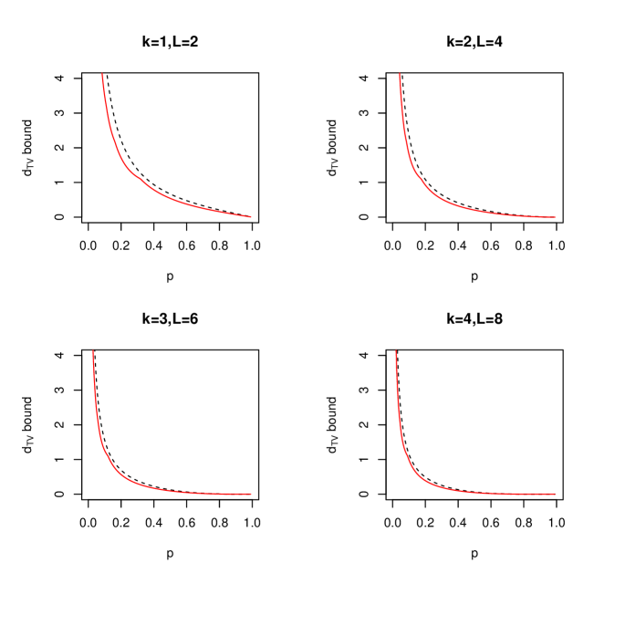
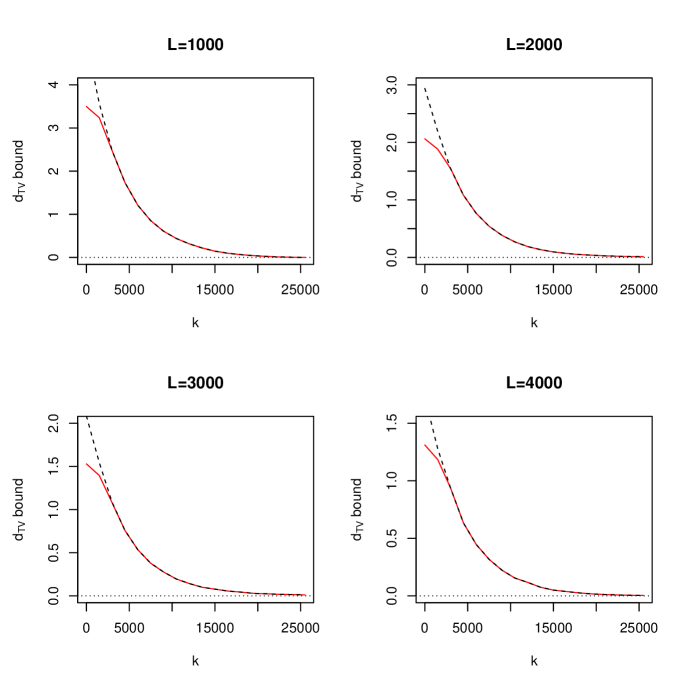
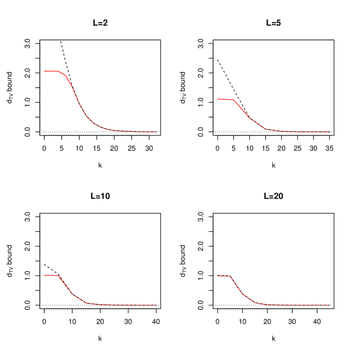
Figure 1 compares the bounds (2.2) (dashed line) and (4.4) (solid line) for different values of , , and . One can see that the new bound is sharper, and that only for larger values of , corresponding to fast-mixing chains, are the two bounds indistinguishable. The horizontal line in Figure 1 marks the obvious bound, because . Note too that for very small values of , both bounds are vacuous, but the new bound has a larger range for being nonvacuous.
The simulations in the remaining two examples rely on the
unbiasedmcmc package of Pierre Jacob, available from:
https://github.com/pierrejacob/unbiasedmcmc/tree/master/vignettes. Additional programs for implementing the new ideas in this paper are available as supplemental material from the authors.
4.2 An Empirical Comparison of the Bounds: Ising Model
The Ising model example follows the setup in Biswas et al. (2019). We consider a square lattice of pixels with values in , and with periodic boundaries. A state of the system is then , and the target probability is defined as , where means that and are pixel values in neighboring sites. This illustration uses the parallel tempering algorithm (PT, see Swendsen and Wang, 1986) coupled with a single site Gibbs (SSG) updating. It is known that larger values of increase the dependence between neighboring sites, and that this “stickiness” leads to slow mixing of the SSG. The target of interest corresponds to and we use 12 chains, each corresponding to a different , with values equally spaced between and . Figure 2 shows the total variation bounds, where that provided by (2.1) is shown as a dashed line and that from (2.16) is shown as a solid line. The bounds are derived for and . For smaller values of , the patterns are similar, but TV bounds are larger for smaller values of . The new bound, (2.16), is computed from parallel runs, and is averaged over independent replicates, while (2.1) is averaged over independent replicates of a single coupled process.
Although the numerical results confirm that our new bound never exceeds the bound of Biswas et al. (2019), unfortunately, in this case, the improvement from our bound is visible only when it is not needed, that is, when both bounds exceed one. Whereas this is a disappointment for our effort to improve the bound with a real gain, it is good news for practitioners, because the bound in Biswas et al. (2019) is a bit simpler to use.
4.3 Comparing Bounds and Estimators: A Logistic Regression Example
To compare the bounds and the unbiased estimators, we follow Biswas et al. (2019) and consider a Bayesian logistic regression model for the German credit data of Lichman (2013). The data consist of binary responses, and covariates, . The response indicates whether the th individual is fit to receive credit () or not (). The logistic regression model frames the probabilistic dependence between the response and covariate as . The prior is set to . Sampling from the posterior distribution is done using the Pólya-Gamma sampler of Polson et al. (2013), using the R programs made available by Biswas et al. (2019) at https://github.com/niloyb/LlagCouplings. In Figure 3, we compare the bound of Biswas et al. (2019) (2.1) (dashed line) with our bound (2.16) (solid line). The bound in (2.1) is averaged over 2000 independent replicates. The new bound is computed from running 50 coupled processes in parallel and averaged over 40 replicates, yielding the same number of runs. The difference between the two bounds is apparent for smaller values of when the new bound is sharper for small values of , but the gain diminishes quickly as increases.
We are also interested in the gains in efficiency for the Monte Carlo estimators when implementing the control variate swindle. Using 500 independent replicates of a single coupled process with lag , we obtain Monte Carlo estimates of the posterior means for the regression coefficients. In Figure 4, we present the relative reduction in variance (RRV), computed as RRV, where is the posterior mean of the regression coefficients, , and and denote the estimated Monte Carlo variances of obtained without and with the control variates, respectively. The left panel shows the RRV when using the single-run estimators (2.4) and (3.1), while the right panel plots the RRV for the mean estimators (3.2) and (3.3). We see clearly that the gain is significant for (left panels), but diminishes when and (right panels), as discussed in Section 3.


5 Can We Do Even Better?
The idea of L-lag coupling has opened multiple avenues for future research. The use of control variates is just one of them. Although the practical gain is small or possibly even negative when we take into account the increased computation when computing the control variates, the theoretical gain is intriguing, because we obtain a theoretically superior bound without imposing any additional assumptions. This naturally raises the question of whether our bound is the best possible without further conditions. We do not know. We do not even know how to study such a question theoretically, because to the best of our knowledge, this is the first time a tighter theoretical bound has been obtained by a better empirical estimator. Whereas seeking other more efficient estimators seems to be a natural direction, we must keep in mind that they would likely incur additional computational costs.
One plausible direction is to go beyond linearly combining mean-zero control variates, although we had no success so far. However, even without seeking better bounds, our current bounds already offer the opportunity to investigate fresh perspectives for optimizing an MCMC kernel using adaptive ideas, and we intend to pursue these in future research.
Acknowledgments
We are grateful to Pierre Jacob for many useful comments and his gracefully patient guidance through the package unbiasedmcmc, allowing us to perform the simulations in our study. We also thank Yves Atchadé, Tamas Papp, Christopher Sherlock, and Lei Sun for their helpful discussions and comments, and the NSERC of Canada (RVC) and NSF of USA (XLM) for their partial research support.
References
- Berthelsen and Møller (2002) Berthelsen, K. K. and Møller, J. (2002). A primer on perfect simulation for spatial point processes. Bull. Braz. Math. Soc. (N.S.) 33, 351–367. Fifth Brazilian School in Probability (Ubatuba, 2001).
- Biswas et al. (2019) Biswas, N., Jacob, P. E. and Vanetti, P. (2019). Estimating convergence of Markov chains with L-lag couplings. In Advances in Neural Information Processing Systems, pp. 7389–7399.
- Corcoran and Schneider (2005) Corcoran, J. N. and Schneider, U. (2005). Pseudo-perfect and adaptive variants of the Metropolis-Hastings algorithm with an independent candidate density. J. Stat. Comput. Simul. 75, 459–475.
- Corcoran and Tweedie (2002) Corcoran, J. N. and Tweedie, R. L. (2002). Perfect sampling from independent Metropolis-Hastings chains. J. Statist. Plann. Inference 104, 297–314.
- Craiu and Lemieux (2007) Craiu, R. V. and Lemieux, C. (2007). Acceleration of the multiple-try Metropolis algorithm using antithetic and stratified sampling. Statistics and Computing 17, 109–120.
- Craiu and Meng (2001) Craiu, R. V. and Meng, X.-L. (2001). Antithetic coupling for perfect sampling. In E. I. George (Ed.), Bayesian Methods, with Applications to Science, Policy and Official Statistics (Proceedings of the ISBA 2000 conference, Hersonnissos, Crete), 99-108. Luxembourg: Office for Official Publications of the European Communities.
- Craiu and Meng (2005) Craiu, R. V. and Meng, X.-L. (2005). Multiprocess parallel antithetic coupling for backward and forward Markov chain Monte Carlo. The Annals of Statistics 33, 661–697.
- Craiu and Meng (2011) Craiu, R. V. and Meng, X.-L. (2011). Perfection within reach: exact MCMC sampling. Handbook of Markov Chain Monte Carlo, 199–226.
- Craiu and Meng (2020) Craiu, R. V. and Meng, X.-L. (2020). Discussion of ”Unbiased Markov chain Monte Carlo with couplings” by Pierre E. Jacob, John O’Leary and Yves F. Atchadé. J. Royal Statist. Society, Series B, 82, 578–581.
- Dobrow and Fill (2003) Dobrow, R. P. and Fill, J. A. (2003). Speeding up the FMMR perfect sampling algorithm: a case study revisited. Random Structures Algorithms 23, 434–452.
- Ensor and Glynn (2000) Ensor, K. B. and Glynn, P. W. (2000). Simulating the maximum of a random walk. Journal of Statistical Planning and Inference 85, 127–135.
- Glynn (2016) Glynn, P. W. (2016). Exact simulation vs exact estimation. In 2016 Winter Simulation Conference (WSC), pp. 193–205. IEEE.
- Glynn and Heidelberger (1991) Glynn, P. W. and Heidelberger, P. (1991). Analysis of parallel replicated simulations under a completion time constraint. ACM Transactions on Modeling and Computer Simulation (TOMACS) 1, 3–23.
- Glynn and Rhee (2014) Glynn, P. W. and Rhee, C.-h. (2014). Exact estimation for Markov chain equilibrium expectations. Journal of Applied Probability 51, 377–389.
- Heng and Jacob (2019) Heng, J. and Jacob, P. E. (2019). Unbiased Hamiltonian Monte Carlo with couplings. Biometrika 106, 287–302.
- Huber (2002) Huber, M. L. (2002). A bounding chain for Swendsen-Wang. Random Structures and Algorithms 22, 43–59.
- Huber (2004) Huber, M. L. (2004). Perfect sampling using bounding chains. Ann. Appl. Probab. 14, 734–753.
- Jacob et al. (2019) Jacob, P. E., Lindsten, F. and Schön, T. B. (2019). Smoothing with couplings of conditional particle filters. Journal of the American Statistical Association, 115, 721–729.
- Jacob et al. (2020) Jacob, P. E., O’Leary, J. and Atchadé, Y. F. (2020). Unbiased Markov chain Monte Carlo with couplings (with discussion). J. Royal Statist. Society, Series B, 82 , 543–600.
- Lichman (2013) Lichman, M. (2013). Uci machine learning repository, 2013.
- Meng (2000) Meng, X. L. (2000). Towards a more general Propp-Wilson algorithm: Multistage backward coupling. In N. Madras (Ed.), Monte Carlo Methods, Volume 26 of Fields Institute Communications, pp. 85–93. American Mathematical Society.
- Møller (1999) Møller, J. (1999). Perfect simulation of conditionally specified models. J. Royal Statist. Society, Series B 61, 251–264.
- Murdoch and Meng (2001) Murdoch, D. J. and Meng, X.-L. (2001). Towards perfect sampling for Bayesian mixture priors. In E. I. George (Ed.), Bayesian Methods, with Applications to Science, Policy and Official Statistics (Proceedings of the ISBA 2000 conference, Hersonnissos, Crete), 381-390. Luxembourg: Office for Official Publications of the European Communities.
- Murdoch and Takahara (2006) Murdoch, D. J. and Takahara, G. (2006). Perfect sampling for queues and network models. ACM Transactions on Modeling and Computer Simulation 16, 76–92.
- Nelson (2016) Nelson, B. L. (2016). ‘Some tactical problems in digital simulation’ for the next 10 years. Journal of Simulation 10, 2–11.
- Polson et al. (2013) Polson, N. G., Scott, J. G. and Windle, J. (2013). Bayesian inference for logistic models using Pólya–Gamma latent variables. Journal of the American Statistical Association 108, 1339–1349.
- Propp and Wilson (1996) Propp, J. G. and Wilson, D. B. (1996). Exact sampling with coupled Markov chains and applications to statistical mechanics. Random Structures and Algorithms 9, 223–252.
- Propp and Wilson (1998) Propp, J. G. and Wilson, D. B. (1998). How to get a perfectly random sample from a generic Markov chain and generate a random spanning tree of a directed graph. J. Algorithms 27, 170–217. 7th Annual ACM-SIAM Symposium on Discrete Algorithms (Atlanta, GA, 1996).
- Stein and Meng (2013) Stein, N. M. and Meng, X.-L. (2013). Practical perfect sampling using composite bounding chains: the Dirichlet-multinomial model. Biometrika 100, 817–830.
- Swendsen and Wang (1986) Swendsen, R. H. and Wang, J.-S. (1986). Replica Monte Carlo simulation of spin-glasses. Physical review letters 57, 2607.
- Thönnes (1999) Thönnes, E. (1999). Perfect simulation of some point processes for the impatient user. Adv. in Appl. Probab. 31, 69–87.
- Van Dyk and Meng (2001) Van Dyk, D. A. and Meng, X.-L. (2001). The art of data augmentation (with discussion). Journal of Computational and Graphical Statistics 10, 1–50.
- Wilson (1998) Wilson, D. B. (1998). Annotated bibliography of perfectly random sampling with Markov chains. In D. Aldous and J. Propp (Eds.), Microsurveys in Discrete Probability, Volume 41 of DIMACS Series in Discrete Mathematics and Theoretical Computer Science, pp. 209–220. American Mathematical Society. Updated versions appear at http://www.dbwilson.com/exact/.
- Yu and Meng (2011) Yu, Y. and Meng, X.-L. (2011). To center or not to center: That is not the question—an Ancillarity–Sufficiency Interweaving Strategy (ASIS) for boosting MCMC efficiency (with discussion). Journal of Computational and Graphical Statistics 20, 531–570.