High-order energy stable schemes of incommensurate phase-field crystal model

Abstract

This article focuses on the development of high-order energy stable schemes for the multi-length-scale incommensurate phase-field crystal model which is able to study the phase behavior of aperiodic structures. These high-order schemes based on the scalar auxiliary variable (SAV) and spectral deferred correction (SDC) approaches are suitable for the $L^{2}$ gradient flow equation, i.e., the Allen-Cahn dynamic equation. Concretely, we propose a second-order Crank-Nicolson (CN) scheme of the SAV system, prove the energy dissipation law, and give the error estimate in the almost periodic function sense. Moreover, we use the SDC method to improve the computational accuracy of the SAV/CN scheme. Numerical results demonstrate the advantages of high-order numerical methods in numerical computations and show the influence of length-scales on the formation of ordered structures.

Kai Jiang^∗ and Wei Si

School of Mathematics and Computational Science

Hunan Key Laboratory for Computation and Simulation in Science and Engineering

Xiangtan University, Hunan, Xiangtan 411105, China

1 Introduction

Aperiodic crystals, such as quasicrystals, are an important class of materials whose Fourier spectra cannot be all expressed by a set of basis vectors over the rational number field. The irrational coefficients give rise to the denseness of Fourier spectra which results in the difficulties in the theoretical study. Theoretically, a multiple characteristic length-scale model which possesses, at least, an irrational scale, has been widely applied to study the formation and thermodynamic stability of the aperiodic structures [1, 6, 13, 10, 14, 7]. The early model could trace back to Bak’s work on three-dimensional icosahedral quasicrystals. Since then, many related models have been proposed to study aperiodic structures, including for multicomponent systems [7]. Among these models, Lifshitz and Petrich (LP) modified the Swift-Hohenberg model and explicitly added an incommensurate two-length-scale potential into a Lyapunov functional to explore quasiperiodic patterns that emerged in Faraday experiments [13]. Recently, Savitz et al. extended the LP model from two-length-scale potential to multiple ($\geq 3$) length-scale potential and studied more kinds of quasicrystals [14]. The $m$-length-scale model actually is an incommensurate multi-length-scale phase-field-crystal (iPFC) model who owns a $4m$ ($m\in\mathbb{N}$) order differential operator and nonlinear term in the energy functional. A high precision computation is helpful to study the phase behaviors of aperiodic structures. In this article, we will pay attention to the development of high-order numerical methods for the iPFC model.

Recently, various numerical methods have been proposed to solve phase-field equations including the convex splitting methods [17], the linear stabilized schemes [16], the invariant energy quadratization (IEQ) [18] and the scalar auxiliary variable (SAV) approaches [15, 11]. The convex splitting method splits the energy functional into the convex and concave parts. The method treats the convex part implicitly and the concave one explicitly to keep the unconditional energy stability. While the application of this method is restricted by the form of the energy functional, such as double-well bulk energy. The linear stabilized scheme adds a penalty term to improve its stability and deals with the nonlinear terms explicitly for implementing it easily. However, such a stabilized approach makes it difficult to design second-order unconditionally energy stable schemes. Assume that the nonlinear part has a lower bound, via introducing an auxiliary variable, the IEQ method transforms the energy functional into a quadratic form to keep the unconditional energy dissipation property. Similarly, the SAV approach introduces a scalar auxiliary variable by supposing the bounded bulk energy and obtains an unconditionally energy stable system. Besides these methods, the spectral deferred correction (SDC) [4, 5] algorithm is an efficient strategy to improve the accuracy of the above schemes. In the paper, we will apply the SAV approach to solve the time-dependent equations and further use the SDC strategy to improve the numerical accuracy.

For aperiodic structures, two kinds of numerical methods, including the crystalline approximant method (CAM) and the projection method (PM) are usually used to discretize the quasiperiodic functions [9]. The CAM uses a big periodic structure to approximate an aperiodic structure and corresponds to the Diophantine approximation problem which studies how to approximate irrational numbers by rational numbers [3]. To evaluate aperiodic structures accurately, the CAM needs an extremely big computational region with an unacceptable computational burden to reduce the error of Diophantine approximation. To avoid the Diophantine approximation problem, the PM accurately describes aperiodic structures based on the fact that the aperiodic structure can be regarded as a periodic crystal in an appropriate higher-dimensional space. The PM uses one higher-dimensional periodic region to capture the essential characteristics and greatly reduces computational complexity.

The rest of the paper is organized as follows. In Section 2, we first outline some useful preliminaries of the almost periodic functions and then present the iPFC model. The energy dissipation principle of the $L^{2}$ gradient flow for the iPFC model in the almost periodic sense is also given. In Section 3, we propose a second-order energy stable scheme for the iPFC model and give the corresponding error estimate. And we use the SDC approach to improve its computational accuracy efficiently. Section 4 presents the convergence rates of these numerical schemes and discusses the advantages of high-order numerical approaches in simulating dynamic evolution. Moreover, we also show the influence of multiple length-scales on the thermodynamic stability of aperiodic structures. There are some conclusions in Section 5.

2 Problem formulation

2.1 Preliminary

Aperiodic structures are space-filling phases without decay. A useful mathematical theory to describe aperiodic structures is the almost periodic function theory which is a generalization of continuous periodic functions. We define the notation of a $d$-dimensional almost periodic function.

Definition 2.1.

Let $f(\bm{r})$ be a real-valued or complex-valued function defined on $\mathbb{R}^{d}$ and let $\epsilon>0$. We say that $\zeta\in\mathbb{R}^{d}$ is an $\epsilon$-almost period of $f$ if

$$|f(\bm{r}-\zeta)-f(\bm{r})|<\epsilon,~{}\mbox{~{}~{}for any ~{}}\bm{r}\in\mathbb{R}^{d}.$$

A function $f$ is almost periodic on $\mathbb{R}^{d}$ if it is continuous and if for every $\epsilon$ there exists a number $L=L(\epsilon,f)$ such that any cube with the side length of $L$ on $\mathbb{R}^{d}$ contains an $\epsilon$-almost period of $f$.

The almost periodic $L^{2}$ inner product is defined by

$$\left<f,g\right>_{AP}=\lim_{R\to\infty}\frac{1}{|Q(R)|}\int_{Q(R)}f(\bm{r}){\color[rgb]{0,0,0}\overline{g(\bm{r})}}\,d\bm{r},$$ (1)

where $Q(R)=[-R,R]^{d}$ and $|Q(R)|$ is the measure of $Q(R)$. It is known that this inner product is well-defined [2]. We denote the corresponding norm by $\left\|\cdot\right\|^{2}_{AP}=\left<\cdot,\cdot\right>_{AP}$. For simplicity, we denote the average spacial integral over the whole space as

$${\mathchoice{{-\mkern-19.0mu\int}}{{-\mkern-16.0mu\int}}{{-\mkern-16.0mu\int}}{{-\mkern-16.0mu\int}}}=\lim_{R\to\infty}\frac{1}{|Q(R)|}\int_{Q(R)}.$$ (2)

Some useful properties of $d$-dimensional almost periodic functions are presented as follows.

Proposition 1.

1. An almost periodic function is uniformly continuous andbounded.

2. If $f(\bm{r})$ and $g(\bm{r})$ are almost periodic functions, then $f(\bm{r})+g(\bm{r})$ and $f(\bm{r})\cdot g(\bm{r})$ are almost periodic functions.

These properties can be easily proven from the one-dimensional results [2].

Theorem 2.2.

If $f(\bm{r})$ and $g(\bm{r})$ are almost periodic functions and differentiable, then the Green’s identity holds in the almost periodic sense, i.e.,

$$\left<f(\bm{r}),\nabla g(\bm{r})\right>_{AP}=-\left<\nabla f(\bm{r}),g(\bm{r})\right>_{AP}.\vspace*{-10pt}$$ (3)

Proof.

Since $f(\bm{r})$ and $g(\bm{r})$ are almost periodic functions, then there exists a constant $M$ such that $\sup\limits_{\bm{r}}\left\{\left|f(\bm{r})\right|,\left|g(\bm{r})\right|\right\}\leq M$. Denote

$$b_{R}=\lim_{R\to\infty}\frac{1}{|Q(R)|}\int_{\partial Q(R)}f(\bm{r})\bm{n}\cdot{\color[rgb]{0,0,0}\overline{g(\bm{r})}}\,ds,$$ (4)

where $\bm{n}$ is the outward normal of $\partial Q(R)$. In the $d$-dimensional space, we have

$$|b_{R}|\leq\lim_{R\to\infty}\frac{M^{2}2d(2R)^{d-1}}{(2R)^{d}}=0.$$ (5)

Therefore, we obtain the desired conclusion by

$$\left<f(\bm{r}),\nabla g(\bm{r})\right>_{AP} ={\mathchoice{{-\mkern-19.0mu\int}}{{-\mkern-16.0mu\int}}{{-\mkern-16.0mu\int}}{{-\mkern-16.0mu\int}}}f(\bm{r})\nabla g(\bm{r})\,d\bm{r}$$ (6)

$$=-{\mathchoice{{-\mkern-19.0mu\int}}{{-\mkern-16.0mu\int}}{{-\mkern-16.0mu\int}}{{-\mkern-16.0mu\int}}}\nabla f(\bm{r})g(\bm{r})\,d\bm{r}=-\left<\nabla f(\bm{r}),g(\bm{r})\right>_{AP}.$$

∎

2.2 Incommensurate phase-field crystal (iPFC) model

The simplest iPFC model may be the LP model which was originally proposed to study the bi-frequency excited Faraday wave [13]. Concretely, the free energy functional of the LP model can be written as

$$F_{LP}[\psi(\bm{r})]={\mathchoice{{-\mkern-19.0mu\int}}{{-\mkern-16.0mu\int}}{{-\mkern-16.0mu\int}}{{-\mkern-16.0mu\int}}}\left\{\frac{c}{2}\left[(\Delta+1)(\Delta+q^{2})\psi\right]^{2}+\left(\frac{\varepsilon}{2}\psi^{2}-\frac{\alpha}{3}\psi^{3}+\frac{1}{4}\psi^{4}\right)\right\}\,d\bm{r},$$ (7)

where $q$ is an irrational number depending on the property of quasiperiodic structures. The essential feature of the energy functional is the existence of two characteristic length-scales, $1$ and $q$, which is a critical factor to stabilize quasi-periodic structures. The LP model has been also used to study the soft-matter quasicrystals [12]. However, this model could be able to globally stabilize the dodecagonal and decagonal rotational quasicrystals [8]. To generalize the iPFC model, Savitz et al. extended the interaction potential from two characteristic length-scales to multiple characteristic length-scales. In particular, the Lyapunov functional of an $m$-length-scale incommensurate system can be written as

$$F[\psi(\bm{r})]={\mathchoice{{-\mkern-19.0mu\int}}{{-\mkern-16.0mu\int}}{{-\mkern-16.0mu\int}}{{-\mkern-16.0mu\int}}}\Bigg{\{}\frac{c}{2}\Big{[}\prod_{j=1}^{m}(\Delta+q_{j}^{2})\psi\Big{]}^{2}+\Big{(}\frac{\varepsilon}{2}\psi^{2}-\frac{\alpha}{3}\psi^{3}+\frac{1}{4}\psi^{4}\Big{)}\Bigg{\}}\,d\bm{r},$$ (8)

where $\psi(\bm{r})$, $\bm{r}\in\mathbb{R}^{d}$ $(d=1,2,3)$, is the order parameter corresponding to the density profile of the system. $q_{j}$ is the $j$-th characteristic length-scale which depends on the property of aperiodic structures. $c$ is a positive model parameter to ensure that the principle wavelengths are near the critical wavelengths. $\varepsilon$ and $\alpha$ are both model parameters related to physical conditions, such as temperature, pressure. To reduce the number of model parameters, the iPFC energy functional can be rescaled by defining $F=c^{2}\mathcal{F}$, $\psi(\bm{r})=\sqrt{c}\phi(\bm{r})$, $\tilde{\varepsilon}=c\varepsilon$, and $\tilde{\alpha}=\sqrt{c}\alpha$. The rescaled functional is

$$\mathcal{F}[\phi(\bm{r})]={\mathchoice{{-\mkern-19.0mu\int}}{{-\mkern-16.0mu\int}}{{-\mkern-16.0mu\int}}{{-\mkern-16.0mu\int}}}\Big{\{}\frac{1}{2}[\mathcal{G}\phi]^{2}+\mathcal{N}(\phi)\Big{\}}\,d\bm{r}=\frac{1}{2}\|\mathcal{G}\phi\|_{AP}^{2}+\left<\mathcal{N}(\phi),1\right>_{AP},$$ (9)

where

$$\mathcal{G}=\prod_{j=1}^{m}(\Delta+q_{j}^{2}),\quad\quad\mathcal{N}(\phi)=\frac{\tilde{\varepsilon}}{2}\phi^{2}-\frac{\tilde{\alpha}}{3}\phi^{3}+\frac{1}{4}\phi^{4}.$$ (10)

To solve the iPFC free energy functional, we consider the following Allen-Cahn dynamic equation

$$\phi_{t} =-\mathcal{W}(\phi),$$ (11)

$$\mathcal{W}(\phi) :=\frac{\delta\mathcal{F}}{\delta\phi}=\mathcal{G}^{2}\phi+\mathcal{N}^{\prime}(\phi).$$

The initial value is $\phi|_{t=0}=\phi_{0}$. From Theorem 2.2, we can prove that the system (11) satisfies the following energy dissipation law

$$\frac{d\mathcal{F}(\phi)}{dt}=\left<\frac{\delta\mathcal{F}}{\delta\phi},\phi_{t}\right>_{AP}=-\left\|\mathcal{W}(\phi)\right\|^{2}_{AP}\leq 0.$$ (12)

Then we impose the following mean zero constraint of order parameter on the iPFC model to ensure the mass conservation

$${\mathchoice{{-\mkern-19.0mu\int}}{{-\mkern-16.0mu\int}}{{-\mkern-16.0mu\int}}{{-\mkern-16.0mu\int}}}\phi(\bm{r})\,d\bm{r}=0.$$ (13)

3 Numerical methods

In this section, we propose the second-order unconditionally energy stable Crank-Nicolson scheme based on the SAV technique, and also give the error analysis. Further, we use the SDC strategy to improve the temporal accuracy of the second-order scheme.

3.1 The scalar auxiliary variable (SAV) approach

Let’s suppose that $F_{1}(\phi)\break=\left<\mathcal{N}(\phi),1\right>_{AP}+C_{1}\geq 0$, where $C_{1}$ is a positive constant. We introduce a scalar auxiliary variable $\mathcal{R}=\sqrt{F_{1}(\phi)}$ to transform (11) into an equivalent system as

$$\phi_{t} =-\mathcal{W}(\phi),$$ (14a)

$$\mathcal{W}(\phi) =\mathcal{G}^{2}\phi+\frac{\mathcal{R}}{\sqrt{F_{1}(\phi)}}\mathcal{N}^{\prime}(\phi),$$ (14b)

$$\mathcal{R}_{t} =\left<\frac{\mathcal{N}^{\prime}(\phi)}{2\sqrt{F_{1}(\phi)}},\phi_{t}\right>_{AP}.$$ (14c)

By taking the almost periodic inner products of (14a) with $\mathcal{W}$, and (14b) with $-\phi_{t}$, multiplying (14c) with $2\mathcal{R}$ and adding them together, we have the following energy dissipation property

$$\frac{d}{dt}\left(\frac{1}{2}\left\|\mathcal{G}\phi\right\|^{2}_{AP}+\mathcal{R}^{2}-C_{1}\right)=-\left\|\mathcal{W}\right\|^{2}_{AP}\leq 0.$$ (15)

The SAV approach can construct high-order unconditionally energy stableschemes. In this section, we discuss a second-order semi-discrete scheme based on the Crank-Nicolson method. Suppose the time interval $[0,T]$ is divided into $N_{T}$ non-overlapping subintervals by the partition $0=t^{0}<t^{1}<\cdots<t^{n}<\cdots<t^{N_{T}}=T$. The time step size is $\tau^{n}=t^{n+1}-t^{n}$. We denote $t^{n}+\tau^{n}/2$ as $t^{n+1/2}$. Let $\phi^{n}=\phi(t^{n})$ and $\mathcal{R}^{n}=\mathcal{R}(t^{n})$.

Scheme 3.1 (SAV/CN).

For $n\geq 1$, given $\phi^{n}$, $\mathcal{R}^{n}$ and $\phi^{n-1}$, $\mathcal{R}^{n-1}$, we update $\phi^{n+1}$ and $\mathcal{R}^{n+1}$ by

$$\frac{\phi^{n+1}-\phi^{n}}{\tau^{n}} =-\mathcal{W}^{n+1/2},$$ (16a)

$$\mathcal{W}^{n+1/2} =\mathcal{G}^{2}\phi^{n+1/2}+\frac{\mathcal{R}^{n+1/2}}{\sqrt{F_{1}(\bar{\phi}^{n+1/2})}}\mathcal{N}^{\prime}(\bar{\phi}^{n+1/2}),$$ (16b)

$$\frac{\mathcal{R}^{n+1}-\mathcal{R}^{n}}{\tau^{n}} =\left<\frac{\mathcal{N}^{\prime}(\bar{\phi}^{n+1/2})}{2\sqrt{F_{1}(\bar{\phi}^{n+1/2})}},\frac{\phi^{n+1}-\phi^{n}}{\tau^{n}}\right>_{AP},$$ (16c)

where $\mathcal{R}^{n+1/2}=(\mathcal{R}^{n+1}+\mathcal{R}^{n})/2$, $\phi^{n+1/2}=(\phi^{n+1}+\phi^{n})/2$ and $\bar{\phi}^{n+1/2}=(3\phi^{n}-\phi^{n-1})/2$.

Theorem 3.1.

The SAV/CN scheme satisfies the following energy dissipation mechanism

$$\mathcal{F}_{SAV/CN}^{n+1}-\mathcal{F}_{SAV/CN}^{n}\leq 0,$$ (17)

where

$$\mathcal{F}_{SAV/CN}^{n}=\frac{1}{2}\left\|\mathcal{G}\phi^{n}\right\|^{2}_{AP}+(\mathcal{R}^{n})^{2}-C_{1}.$$ (18)

Proof.

We take the almost periodic inner products of (16a) with $\tau^{n}\mathcal{W}^{n+1/2}$, and (16b) with $-(\phi^{n+1}-\phi^{n})$.

$$\left<\phi^{n+1}-\phi^{n},\mathcal{W}^{n+1/2}\right>_{AP}=-\left\|\mathcal{W}^{n+1/2}\right\|^{2}_{AP},$$ (19)

$$-\left<\phi^{n+1}-\phi^{n},\mathcal{W}^{n+1/2}\right>_{AP} =-\left<\phi^{n+1}-\phi^{n},\mathcal{G}^{2}\phi^{n+1/2}\right>_{AP}$$ (20)

$$-\left<\phi^{n+1}-\phi^{n},\frac{\mathcal{R}^{n+1/2}}{\sqrt{F_{1}(\bar{\phi}^{n+1/2})}}\mathcal{N}^{\prime}(\bar{\phi}^{n+1/2})\right>_{AP}.$$

Multiplying (16c) with $2\mathcal{R}^{n+1/2}$ yields

$$2\mathcal{R}^{n+1/2}(\mathcal{R}^{n+1}-\mathcal{R}^{n})=\left<\frac{\mathcal{R}^{n+1/2}}{\sqrt{F_{1}(\bar{\phi}^{n+1/2})}}\mathcal{N}^{\prime}(\bar{\phi}^{n+1/2}),\phi^{n+1}-\phi^{n}\right>_{AP}.$$ (21)

Adding (19), (20) and (21) together, we obtain

$$2\mathcal{R}^{n+1/2}(\mathcal{R}^{n+1}-\mathcal{R}^{n})=-\left<\phi^{n+1}-\phi^{n},\mathcal{G}^{2}\phi^{n+1/2}\right>_{AP}-\left\|\mathcal{W}^{n+1/2}\right\|^{2}_{AP}.$$ (22)

Since $\mathcal{R}^{n+1/2}=(\mathcal{R}^{n+1}+\mathcal{R}^{n})/2$ and $\phi^{n+1/2}=(\phi^{n+1}+\phi^{n})/2$, (22) can be recast as

$$\frac{1}{2}\left(\left\|\mathcal{G}\phi^{n+1}\right\|^{2}_{AP}-\left\|\mathcal{G}\phi^{n}\right\|^{2}_{AP}\right)+(\mathcal{R}^{n+1})^{2}-(\mathcal{R}^{n})^{2}=-\left\|\mathcal{W}^{n+1/2}\right\|^{2}_{AP}\leq 0.$$ (23)

The desired conclusion is obtained from the above equation. ∎

Remark 3.1.

It is noted that the modified energy $\mathcal{F}_{SAV/CN}^{n}$ is different from the original energy $\mathcal{F}(\phi^{n})$ since $\mathcal{R}^{n}$ is obtained from the iteration process.

Remark 3.2 (The implementation of the SAV/CN scheme).

Denote

$$u(t^{n+1/2})=\frac{\mathcal{N}^{\prime}(\phi(t^{n+1/2}))}{\sqrt{F_{1}(\phi(t^{n+1/2}))}},\quad\quad u^{n+1/2}=\frac{\mathcal{N}^{\prime}(\bar{\phi}^{n+1/2})}{\sqrt{F_{1}(\bar{\phi}{n+1/2})}}.$$ (24)

Substituting (16b) and (16c) into (16a), we obtain

$$\frac{\phi^{n+1}-\phi^{n}}{\tau^{n}}=-\left[\mathcal{G}^{2}\phi^{n+1/2}+u^{n+1/2}\left(\mathcal{R}^{n}+\frac{1}{4}\left<u^{n+1/2},\phi^{n+1}-\phi^{n}\right>_{AP}\right)\right].$$ (25)

Eqn. (25) can be rewritten as

$$\quad(I+\frac{\tau^{n}}{2}\mathcal{G}^{2})\phi^{n+1}+\frac{\tau^{n}}{4}u^{n+1/2}\left<u^{n+1/2},\phi^{n+1}\right>_{AP}$$ (26)

$$=(I-\frac{\tau^{n}}{2}\mathcal{G}^{2})\phi^{n}-\tau^{n}\mathcal{R}^{n}u^{n+1/2}+\frac{\tau^{n}}{4}\left<u^{n+1/2},\phi^{n}\right>_{AP}u^{n+1/2}.$$

Taking the almost periodic inner product with $(I+\frac{1}{2}\tau^{n}\mathcal{G}^{2})^{-1}u^{n+1/2}$ leads to

$$\left<u^{n+1/2},\phi^{n+1}\right>_{AP}+\frac{\tau^{n}}{4}\gamma^{n}\left<u^{n+1/2},\phi^{n+1}\right>_{AP}=\left<u^{n+1/2},(I+\frac{\tau^{n}}{2}\mathcal{G}^{2})^{-1}c^{n}\right>_{AP},$$ (27)

where

$$\gamma^{n} =\left<u^{n+1/2},(I+\frac{\tau^{n}}{2}\mathcal{G}^{2})^{-1}u^{n+1/2}\right>_{AP},$$ (28)

$$c^{n} =(I-\frac{\tau^{n}}{2}\mathcal{G}^{2})\phi^{n}-\tau^{n}\mathcal{R}^{n}u^{n+1/2}+\frac{\tau^{n}}{4}\left<u^{n+1/2},\phi^{n}\right>_{AP}u^{n+1/2}.$$ (29)

From (27), we get

$$\left<u^{n+1/2},\phi^{n+1}\right>_{AP}=\frac{\left<u^{n+1/2},(I+\frac{1}{2}\tau^{n}\mathcal{G}^{2})^{-1}c^{n}\right>_{AP}}{I+\frac{1}{4}\tau^{n}\gamma^{n}}.$$ (30)

Then we can directly calculate $\phi^{n+1}$ via (26) and (30).

3.2 Error estimate

In this section, we will derive the error estimate of the SAV/CN scheme 3.1. Denote $e^{n}=\phi^{n}-\phi(t^{n})$, $w^{n+1}=\mathcal{W}^{n+1}-\mathcal{W}(t^{n+1})$, and $r^{n}=\mathcal{R}^{n}-\mathcal{R}(t^{n})$, we have

Theorem 3.2.

For the Allen-Cahn dynamic equation, assume that $\phi^{0}$ is almost periodic and $\left\|\phi_{t}\right\|^{2}_{AP}$ is bounded. Considering a uniform time partition, i.e., $\tau=\tau^{k},k\leq N_{T}$, we have

$$\left\|\mathcal{G}e^{k}\right\|^{2}_{AP}+(r^{k})^{2}\leq C\tau^{4}\int_{0}^{t^{k}}\left(\left\|\phi_{ttt}(s)\right\|^{2}_{AP}+|r_{ttt}(s)|^{2}\right)ds,$$ (31)

where the constant $C$ is independent on $\tau$.

Proof.

Let’s subtract (14) from (16) at $t^{n+1/2}$

$$e^{n+1}-e^{n}=-\tau w^{n+1/2}+T_{1}^{n+1/2},$$ (32)

$$w^{n+1/2}=\mathcal{G}^{2}e^{n+1/2}+\mathcal{R}^{n+1/2}u^{n+1/2}-\mathcal{R}(t^{n+1/2})u(t^{n+1/2}),$$ (33)

$$r^{n+1}-r^{n} =\frac{1}{2}\left<u^{n+1/2},\phi^{n+1}-\phi^{n}\right>_{AP}$$ (34)

$$\quad-\frac{1}{2}\left<u(t^{n+1/2}),\tau\phi_{t}(t^{n+1/2})\right>_{AP}+T_{2}^{n+1/2},$$

where the truncation errors are given by

$$T_{1}^{n+1/2} =\tau\phi_{t}(t^{n+1/2})-\left(\phi(t^{n+1})-\phi(t^{n})\right),$$ (35)

$$T_{2}^{n+1/2} =\tau\mathcal{R}_{t}(t^{n+1/2})-\left(\mathcal{R}(t^{n+1})-\mathcal{R}(t^{n})\right).$$ (36)

With the Taylor expansion, the truncation errors can be rewritten as

$$T_{1}^{n+1/2} =\frac{1}{2}\int_{t^{n+1}}^{t^{n+1/2}}(t^{n+1}-s)^{2}\phi_{ttt}(s)ds-\frac{1}{2}\int_{t^{n}}^{t^{n+1/2}}(t^{n}-s)^{2}\phi_{ttt}(s)ds,$$ (37)

$$T_{2}^{n+1/2} =\frac{1}{2}\int_{t^{n+1}}^{t^{n+1/2}}(t^{n+1}-s)^{2}\mathcal{R}_{ttt}(s)ds-\frac{1}{2}\int_{t^{n}}^{t^{n+1/2}}(t^{n}-s)^{2}\mathcal{R}_{ttt}(s)ds.$$ (38)

Firstly, making the almost periodic inner product of (32) with $w^{n+1/2}$ yields

$$\left<e^{n+1}-e^{n},w^{n+1/2}\right>_{AP}+\tau\left\|w^{n+1/2}\right\|^{2}_{AP}=\left<T_{1}^{n+1/2},w^{n+1/2}\right>_{AP}.$$ (39)

Then its right-hand term can be bounded by

$$\left<T_{1}^{n+1/2},w^{n+1/2}\right>_{AP}\leq\frac{\tau}{2}\left\|w^{n+1/2}\right\|^{2}_{AP}+\frac{C}{\tau}\left\|T_{1}^{n+1/2}\right\|^{2}_{AP}$$ (40)

$$\leq\frac{\tau}{2}\left\|w^{n+1/2}\right\|^{2}_{AP}+C\tau^{4}\int_{t^{n}}^{t^{n+1}}\left\|\phi_{ttt}(s)\right\|^{2}_{AP}ds.$$

Secondly, by taking the almost periodic inner products of (33) with $-(e^{n+1}-e^{n})$, we obtain

$$-\left<w^{n+1/2},e^{n+1}-e^{n}\right>_{AP}=-\frac{1}{2}\left(\left\|\mathcal{G}e^{n+1}\right\|^{2}_{AP}-\left\|\mathcal{G}e^{n}\right\|^{2}_{AP}\right)$$ (41)

$$\quad\quad\quad\quad\quad-\left<\mathcal{R}^{n+1/2}u^{n+1/2}-\mathcal{R}(t^{n+1/2})u(t^{n+1/2}),e^{n+1}-e^{n}\right>_{AP}.$$

Without the minus sign, the second term on the right-hand side in the above equation can be transformed into

$$\quad\left<\mathcal{R}^{n+1/2}u^{n+1/2}-\mathcal{R}(t^{n+1/2})u(t^{n+1/2}),e^{n+1}-e^{n}\right>_{AP}$$ (42)

$$=r^{n+1/2}\left<u^{n+1/2},e^{n+1}-e^{n}\right>_{AP}$$

$$\quad+\mathcal{R}(t^{n+1/2})\left<u^{n+1/2}-u(t^{n+1/2}),e^{n+1}-e^{n}\right>_{AP}.$$

Note that $|\mathcal{R}(t)|\leq C$ and

$$\|u^{n+1/2}-u(t^{n+1/2})\|_{AP} \leq C\|\mathcal{N}^{\prime}(\bar{\phi}^{n+1/2})-\mathcal{N}^{\prime}(\phi(t^{n+1/2}))\|_{AP}$$ (43)

$$\leq C\left(\|e^{n}\|_{AP}+\|e^{n-1}\|_{AP}\right).$$

The last term on the right-hand side of (42) can be estimated by

$$\quad\mathcal{R}(t^{n+1/2})\left<u^{n+1/2}-u(t^{n+1/2}),e^{n+1}-e^{n}\right>_{AP}$$ (44)

$$=\mathcal{R}(t^{n+1/2})\left<u^{n+1/2}-u(t^{n+1/2}),-\tau w^{n+1/2}+T_{1}^{n+1/2}\right>_{AP}$$

$$\leq\frac{\tau}{2}\left\|w^{n+1/2}\right\|^{2}_{AP}+C\tau\left\|u^{n+1/2}-u(t^{n+1/2})\right\|^{2}_{AP}+\frac{C}{\tau}\left\|T_{1}^{n+1/2}\right\|^{2}_{AP}$$

$$\leq\frac{\tau}{2}\left\|w^{n+1/2}\right\|^{2}_{AP}+C\tau\left(\left\|e^{n}\right\|^{2}_{AP}+\left\|e^{n-1}\right\|^{2}_{AP}\right)$$

$$\quad+C\tau^{4}\int_{t^{n}}^{t^{n+1}}\left\|\phi_{ttt}(s)\right\|^{2}_{AP}ds.$$

Thirdly, multiplying the both sides of (34) by $2r^{n+1/2}$, we obtain

$$(r^{n+1})^{2}-(r^{n})^{2}=r^{n+1/2}\left<u^{n+1/2},\phi^{n+1}-\phi^{n}\right>_{AP}$$ (45)

$$\quad\quad\quad\quad\quad-r^{n+1/2}\left<u(t^{n+1/2}),\tau\phi_{t}(t^{n+1/2})\right>_{AP}+2r^{n+1/2}T_{2}^{n+1/2}.$$

The first two terms on the right-hand side of (45) can be rewritten as

$$\quad r^{n+1/2}\left<u^{n+1/2},\phi^{n+1}-\phi^{n}\right>_{AP}-r^{n+1/2}\left<u(t^{n+1/2}),\tau\phi_{t}(t^{n+1/2})\right>_{AP}$$ (46)

$$=r^{n+1/2}\left<u^{n+1/2},e^{n+1}-e^{n}\right>_{AP}-r^{n+1/2}\left<u(t^{n+1/2}),T_{1}^{n+1/2}\right>_{AP}$$

$$\quad+r^{n+1/2}\left<u^{n+1/2}-u(t^{n+1/2}),\phi(t^{n+1})-\phi(t^{n})\right>_{AP},$$

where the last two terms on the right-hand side satisfy

$$-r^{n+1/2}\left<u(t^{n+1/2}),T_{1}^{n+1/2}\right>_{AP} \leq C\tau\left((r^{n+1})^{2}+(r^{n})^{2}\right)$$ (47)

$$\quad+C\tau^{4}\int_{t^{n}}^{t^{n+1}}\left\|\phi_{ttt}(s)\right\|^{2}_{AP}ds,$$

and

$$\quad r^{n+1/2}\left<u^{n+1/2}-u(t^{n+1/2}),\phi(t^{n+1})-\phi(t^{n})\right>_{AP}$$ (48)

$$\leq C\tau\left\|\phi_{t}\right\|^{2}_{AP}\left((r^{n+1/2})^{2}+\left\|u^{n+1/2}-u(t^{n+1/2})\right\|^{2}_{AP}\right)$$

$$\leq C\tau\left((r^{n+1})^{2}+(r^{n})^{2}+\left\|e^{n}\right\|^{2}_{AP}+\left\|e^{n-1}\right\|^{2}_{AP}\right).$$

Therefore the last term on the right-hand side of (45) can be bounded by

$$2r^{n+1/2}T_{2}^{n+1/2}\leq C\tau\left((r^{n+1})^{2}+(r^{n})^{2}\right)+C\tau^{4}\int_{t^{n}}^{t^{n+1}}\left|r_{ttt}(s)\right|^{2}ds.$$ (49)

With the above estimates, adding (39), (41) and (45) together leads to

$$\quad\frac{1}{2}\left(\left\|\mathcal{G}e^{n+1}\right\|^{2}_{AP}-\left\|\mathcal{G}e^{n}\right\|^{2}_{AP}\right)+(r^{n+1})^{2}-(r^{n})^{2}$$ (50)

$$\leq C\tau\left(\left\|e^{n}\right\|^{2}_{AP}+\left\|e^{n-1}\right\|^{2}_{AP}+(r^{n+1})^{2}+(r^{n})^{2}\right)$$

$$\quad+C\tau^{4}\int_{t^{n}}^{t^{n+1}}\left\|\phi_{ttt}(s)\right\|^{2}_{AP}ds+C\tau^{4}\int_{t^{n}}^{t^{n+1}}\left|r_{ttt}(s)\right|^{2}ds.$$

Then we obtain the desired conclusion by summing over $n$, $n=0,1,\cdots,k-1$, and using the Gronwall inequality. ∎

3.3 Spectral deferred correction (SDC) approach

The SDC approach [4, 5] is an efficient method to improve the numerical precision for an existing scheme using spectral collocation points. Firstly, we introduce the basic idea of the SDC method. Integrating both sides of the Eqn. (11) with respect to $t$, we have

$$\phi(t)=\phi(0)-\int_{0}^{t}\mathcal{W}(\phi(\tau))\,d\tau.$$ (51)

Suppose the approximation solution $\phi_{[0]}(t)$ has been calculated by some numerical schemes. Then we define the residual $R_{[0]}(t)$ and the error $\epsilon_{[0]}(t)$ as

$$R_{[0]}(t)=\phi(0)-\int_{0}^{t}\mathcal{W}(\phi_{[0]}(\tau))\,d\tau-\phi_{[0]}(t),$$ (52)

$$\epsilon_{[0]}(t)=\phi(t)-\phi_{[0]}(t).$$ (53)

Replacing (53) into (51) yields

$$\phi(t)=\phi(0)-\int_{0}^{t}\mathcal{W}(\phi_{[0]}(\tau)+\epsilon_{[0]}(\tau))\,d\tau.$$ (54)

Then we insert (54) into (53) and subtract (52)

$$\epsilon_{[0]}(t)-R_{[0]}(t)=-\int_{0}^{t}\mathcal{W}(\phi_{[0]}(\tau)+\epsilon_{[0]}(\tau))d\tau+\int_{0}^{t}\mathcal{W}(\phi_{[0]}(\tau))d\tau.$$ (55)

By taking the derivative of both sides of the above equation, we obtain

$$\frac{d\epsilon_{[0]}(t)}{dt}=-\mathcal{W}(\phi_{[0]}(t)+\epsilon_{[0]}(t))+\mathcal{W}(\phi_{[0]}(t))+\frac{dR_{[0]}(t)}{dt}.$$ (56)

Then, we apply the SDC approach into the second-order SAV/CN scheme to improve the numerical accuracy. We denote this strategy as SAV/CN+SDC. To calculate the integral precisely, we adopt the following Chebyshev nodes,

$$t^{n}=\frac{T}{2}-\frac{T}{2}\cos\left(\frac{n\pi}{N_{T}}\right),~{}~{}n=0,1,\cdots,N_{T}.$$ (57)

The time step size is $\tau^{n}=t^{n+1}-t^{n}$. To obtain the approximation solution $\phi_{[0]}(t)$, we rewrite the SAV/CN scheme as

$$\frac{\phi_{[0]}^{n+1}-\phi_{[0]}^{n}}{\tau^{n}} =-\mathcal{W}_{[0]}^{n+1/2},$$

$$\mathcal{W}_{[0]}^{n+1/2} =\mathcal{G}^{2}\phi_{[0]}^{n+1/2}+\frac{\mathcal{R}_{[0]}^{n+1/2}}{\sqrt{F_{1}(\bar{\phi}_{[0]}^{n+1/2})}}\mathcal{N}^{\prime}(\bar{\phi}_{[0]}^{n+1/2}),$$ (58)

$$\frac{\mathcal{R}_{[0]}^{n+1}-\mathcal{R}_{[0]}^{n}}{\tau^{n}} =\left<\frac{\mathcal{N}^{\prime}(\bar{\phi}_{[0]}^{n+1/2})}{2\sqrt{F_{1}(\bar{\phi}_{[0]}^{n+1/2})}},\frac{\phi_{[0]}^{n+1}-\phi_{[0]}^{n}}{\tau^{n}}\right>_{AP},$$

where $\phi_{[0]}^{0}=\phi^{0}$, $\mathcal{R}_{[0]}^{n+1/2}=(\mathcal{R}_{[0]}^{n+1}+\mathcal{R}_{[0]}^{n})/2$, $\phi_{[0]}^{n+1/2}=(\phi_{[0]}^{n+1}+\phi_{[0]}^{n})/2$ and $\bar{\phi}_{[0]}^{n+1/2}=(3\phi_{[0]}^{n}-\phi_{[0]}^{n-1})/2$. We adopt a similar strategy to discretize (56) as follows

$$\frac{\epsilon_{[0]}^{n+1}-\epsilon_{[0]}^{n}}{\tau^{n}} =-\mathcal{W}_{[0]}^{n+1/2,\epsilon}+\mathcal{W}_{[0]}^{n+1/2}+\frac{R_{[0]}^{n+1}-R_{[0]}^{n}}{\tau^{n}},$$ (59a)

$$\mathcal{W}_{[0]}^{n+1/2,\epsilon} =\mathcal{G}^{2}\phi_{[0]}^{n+1/2,\epsilon}+\frac{\mathcal{R}_{[0]}^{n+1/2}}{\sqrt{F_{1}(\bar{\phi}_{[0]}^{n+1/2})}}\mathcal{N}^{\prime}(\bar{\phi}_{[0]}^{n+1/2,\epsilon}),$$ (59b)

where $\epsilon_{[0]}^{0}=\phi(0)-\phi_{[0]}^{0}=0$, $\phi_{[0]}^{n+1/2,\epsilon}=\phi_{[0]}^{n+1/2}+\epsilon_{[0]}^{n+1/2}$, and $\bar{\phi}_{[0]}^{n+1/2,\epsilon}=\bar{\phi}_{[0]}^{n+1/2}+\bar{\epsilon}_{[0]}^{n+1/2}$. Substituting (58) and (59b) into (59a) and eliminating the residual by (52), we obtain the following linear solvable equation

$$\left(I+\frac{\tau^{n}}{2}\mathcal{G}^{2}\right)\epsilon_{[0]}^{n+1}=\left(I-\frac{\tau^{n}}{2}\mathcal{G}^{2}\right)\epsilon_{[0]}^{n}-\int_{t^{n}}^{t^{n+1}}\mathcal{W}(\phi_{[0]}(\tau^{n}))d\tau^{n}$$ (60)

$$\quad-\phi_{[0]}^{n+1}+\phi_{[0]}^{n}-\tau^{n}\frac{\mathcal{R}_{[0]}^{n+1/2}}{\sqrt{F_{1}(\bar{\phi}_{[0]}^{n+1/2})}}\left\{\mathcal{N}^{\prime}(\bar{\phi}_{[0]}^{n+1/2,\epsilon})-\mathcal{N}^{\prime}(\bar{\phi}_{[0]}^{n+1/2})\right\}.$$

A more accurate solution can be updated by

$$\phi_{[1]}^{n+1}=\phi_{[0]}^{n+1}+\epsilon_{[0]}^{n+1}.$$ (61)

3.4 The projection method (PM) discretization

The PM is an accurate approach in computing aperiodic structures that can avoid the Diophantine approximation error. The PM is based on the fact that the $d$-dimensional aperiodic structure can be embedded into an $n$-dimensional periodic structure $(n\geq d)$. The dimensionality $n$ is determined by the spectrum structures of the aperiodic structures. In particular, $n$ is the number of linearly independent vectors over the rational number field which span the spectrum. In the PM, the $d$-dimensional order parameter $\phi(\bm{r})$ can be expanded as

$$\phi(\bm{r})=\sum_{\bm{h}\in\mathbb{Z}^{n}}\hat{\phi}(\bm{h})e^{i[(\mathcal{P}\cdot\mathbf{Bh})^{T}\cdot\bm{r}]},~{}~{}~{}\bm{r}\in\mathbb{R}^{d}.$$ (62)

where $\mathbf{B}\in\mathbb{R}^{n\times n}$ is an invertible matrix related to the $n$-dimensional primitive reciprocal lattice. The projection matrix $\mathcal{P}\in\mathbb{R}^{d\times n}$ depends on the property of aperiodic structures. If we consider $d$-dimensional periodic structures, the projection matrix degenerates to a $d$-order identity matrix. Therefore, the PM provides a unified framework in calculating periodic and aperiodic crystals. More details about the PM can refer to [9]. The Fourier coefficient $\hat{\phi}(\bm{h})$ satisfies

$$X:=\left\{(\hat{\phi}(\bm{h}))_{\bm{h}\in\mathbb{Z}^{n}}:\hat{\phi}(\bm{h})\in\mathbb{C},~{}\sum_{\bm{h}\in\mathbb{Z}^{n}}|\hat{\phi}(\bm{h})|<\infty\right\}.$$ (63)

In practice, let $\mathbf{N}=(N_{1},N_{2},\dots,N_{n})\in\mathbb{N}^{n}$, and

$$X_{\mathbf{N}}:=\{\hat{\phi}(\bm{h})\in X:\hat{\phi}(\bm{h})=0,~{}\mbox{for all}~{}|h_{j}|>N_{j}/2,~{}j=1,2,\dots,n\}.$$ (64)

The number of elements in the set is $N=(N_{1}+1)(N_{2}+1)\cdots(N_{n}+1)$. Using the PM, the SAV/CN scheme of full discretization reads

$$\hat{\phi}^{n+1}(\bm{h})-\hat{\phi}^{n}(\bm{h}) =-\tau\widehat{\mathcal{W}}^{nh}(\bm{h}),$$ (65)

$$\widehat{\mathcal{W}}^{nh}(\bm{h}) =\frac{1}{2}\prod_{j=1}^{m}[q_{j}^{2}-(\mathcal{P}\mathbf{Bh})^{T}(\mathcal{P}\mathbf{Bh})]^{2}[\hat{\phi}^{n+1}(\bm{h})+\hat{\phi}^{n}(\bm{h})]$$

$$\quad+\frac{\mathcal{R}^{n+1}+\mathcal{R}^{n}}{2\sqrt{F_{1}^{nh}[\hat{\Phi}]}}\widehat{\mathcal{N}^{\prime}}^{nh}(\bm{h}),$$

$$\mathcal{R}^{n+1}-\mathcal{R}^{n} =\sum_{\bm{h}_{1}+\bm{h}_{2}=\bm{0}}\frac{\widehat{\mathcal{N}^{\prime}}^{nh}(\bm{h}_{1})}{2\sqrt{F_{1}^{nh}[\hat{\Phi}]}}[\hat{\phi}^{n+1}(\bm{h}_{2})-\hat{\phi}^{n}(\bm{h}_{2})],$$

where

$$\widehat{\mathcal{N}^{\prime}}^{nh}(\bm{h}) =\tilde{\varepsilon}\hat{\phi}^{nh}(\bm{h})-\tilde{\alpha}\sum_{\bm{h}_{1}+\bm{h}_{2}=\bm{h}}\hat{\phi}^{nh}(\bm{h}_{1})\hat{\phi}^{nh}(\bm{h}_{2})$$ (66)

$$\quad+\sum_{\bm{h}_{1}+\bm{h}_{2}+\bm{h}_{3}=\bm{h}}\hat{\phi}^{nh}(\bm{h}_{1})\hat{\phi}^{nh}(\bm{h}_{2})\hat{\phi}^{nh}(\bm{h}_{3}),$$

$$F_{1}^{nh}[\hat{\Phi}] =\frac{\tilde{\varepsilon}}{2}\sum_{\bm{h}_{1}+\bm{h}_{2}=\bm{0}}\hat{\phi}^{nh}(\bm{h}_{1})\hat{\phi}^{nh}(\bm{h}_{2})-\frac{\tilde{\alpha}}{3}\sum_{\bm{h}_{1}+\bm{h}_{2}+\bm{h}_{3}=\bm{0}}\hat{\phi}^{nh}(\bm{h}_{1})\hat{\phi}^{nh}(\bm{h}_{2})\hat{\phi}^{nh}(\bm{h}_{3})$$

$$\quad+\frac{1}{4}\sum_{\bm{h}_{1}+\bm{h}_{2}+\bm{h}_{3}+\bm{h}_{4}=\bm{0}}\hat{\phi}^{nh}(\bm{h}_{1})\hat{\phi}^{nh}(\bm{h}_{2})\hat{\phi}^{nh}(\bm{h}_{3})\hat{\phi}^{nh}(\bm{h}_{4})+C_{1},$$

$$\hat{\phi}^{nh}(\bm{h}) =\frac{3\hat{\phi}^{n+1}(\bm{h})-\hat{\phi}^{n}(\bm{h})}{2}.$$

In the above equations, the nonlinear terms are $n$-dimensional convolutions in the Fourier space. Directly computing them is extremely expensive. To avoid this, we use the pseudospectral method through the $n$-dimensional fast Fourier transformation to compute them efficiently in the $n$-dimensional time domain by simple multiplication. The mass conservation constraint (13) can be satisfied through

$$e_{1}^{T}\hat{\Phi}=0,$$ (67)

where $e_{1}=(1,0,\cdots,0)^{T}\in\mathbb{R}^{N}$.

4 Numerical results

In this section, we present several numerical examples to verify the accuracy of the SAV/CN and SAV/CN+SDC schemes and to illustrate the advantages of the higher-order scheme in dynamic evolution. We also show the influence of multiple length-scales on the thermodynamic stability of aperiodic structures.

4.1 Accuracy

In this subsection, we take the two characteristic length scale iPFC model in one-dimensional space to test the numerical accuracy of the SAV/CN and SAV/CN+SDC schemes. The model parameters are set as $q_{1}=\sqrt{2}$, $q_{2}=\sqrt{3}$, $\tilde{\varepsilon}=10$ and $\tilde{\alpha}=4$. The computational domain is $[0,2\pi]$. Correspondingly, the projection matrix $\mathcal{P}$ and $\mathbf{B}$ in the PM both are $1$. The initial data is chosen as $\phi(x,0)=\sin(x)$. We check the temporal accuracy by taking the space discretization $N=128$. The numerical solution of $N_{T}=2048$ is set as the reference solution. Tab. 1 shows the errors and convergence rates of the SAV/CN and SAV/CN+SDC schemes at $T=0.2$. One can observe that the numerical accuracy of the SAV/CN scheme is second-order and can be improved to fourth-order by the SDC approach.

Table 1: Errors and convergence rates of the SAV/CN and SAV/CN+SDC schemes for the Allen-Cahn equation. The numerical solution of $N_{T}=2048$ is regarded as the reference value.

		64	128	256	512
SAV/CN	Error	4.75E-3	1.17E-3	2.91E-4	7.17E-5
	Rate	-	2.01	2.02	2.07
SAV/CN + SDC	Error	1.16E-5	6.78E-7	4.04E-8	2.46E-9
	Rate	-	4.07	4.03	4.02

4.2 Dynamic evolution

In this subsection, we simulate the dynamic process of $2$-dimensional dodecagonal quasicrystal (DDQC) using the iPFC model with two length-scales. The model parameters are $q_{1}=1$, $q_{2}=2\cos(\pi/12)$, $\tilde{\varepsilon}=-2$ and $\tilde{\alpha}=2$. The initial value is the DDQC whose spectral distribution and real morphology are shown in Fig. 1. The big blue dot represents the origin and the others are the $24$ basic Fourier modes located on the circles of radii $q_{1}$ and $q_{2}$, respectively.

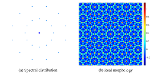
Figure 1: The spectral distribution and the corresponding real morphology of the initial value.

When calculating the DDQC, we adopt the PM to discretize the spatial functions in $4$-dimensional space with $24^{4}$ trigonometric functions. The $24^{4}$ basis functions bring a negligible spatial error comparing the temporal error. The projection matrix in the PM is

$$\mathcal{P}=\left(\begin{array}[]{cccc}1&\cos(\pi/6)&\cos(\pi/3)&0\\ 0&\sin(\pi/6)&\sin(\pi/3)&1\end{array}\right),$$ (68)

and the $\mathbf{B}$ is a 4-order identity matrix.

We use the second-order SAV/CN scheme with $N_{T}=256$ to simulate the dynamic evolution for the DDQC. Fig. 2 shows the change tendency of the energy value. The corresponding morphologies at $t=0,50,100,150,200$ are presented in Fig. 3. As one can see, the proposed scheme satisfies the energy dissipation law. It should be noted that the value $C_{1}$ in the SAV approach plays an important role in computational simulations. In our computation, the $C_{1}$ chosen as $10^{16}$ which maintains the consistency of original and modified energy values.

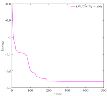
Figure 2: The time evolution of energy which is obtained by the SAV/CN scheme in the case of $N_{T}=256$. The model parameters are $q_{1}=1$, $q_{2}=2\cos(\pi/12)$, $\tilde{\varepsilon}=-2$ and $\tilde{\alpha}=2$.

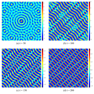
Figure 3: The morphologies of dynamic evolution in Fig. 2. Snapshots are taken at $t=50,~{}100,~{}150,~{}200$, respectively.

To show the role of the high-order methods in dynamic evolution, we give the reference energy $E_{s}$ which is calculated by the SAV/CN+SDC scheme in the case of $N_{T}=2048$. Using the reference value as the baseline, Fig. 4 shows the energy difference of the SAV/CN scheme with $N_{T}=64,~{}128,~{}256$ and SAV/CN+SDC method with $N_{T}=32$. With the increase of the temporal discretization $N_{T}$, the energy difference decreases. However, the energy value obtained by the fourth-order SAV/CN+SDC scheme with $N_{T}=32$ is closer to the reference value than that of the SAV/CN scheme. It is demonstrated that the higher-order method shows more accurate results with less time discretization points in the dynamic simulation.

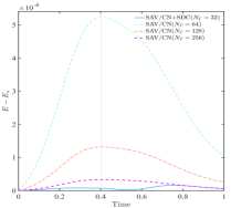
Figure 4: The difference between the numerical energy values and the reference value $E_{s}$. The numerical energy values are computed by the two methods: SAV/CN and SAV/CN+SDC. The reference energy value is obtained by the SAV/CN+SDC method in the case of $N_{T}=2048$. The model parameters are $q_{1}=1$, $q_{2}=2\cos(\pi/12)$, $\tilde{\varepsilon}=-2$ and $\tilde{\alpha}=2$.

We also give the morphologies of the crucial moment $t=0.4025$ in Fig. 5. The morphology of the reference solution is also set as a reference value to clearly illustrate the differences. And the conclusions from these results are consistent with the energy evolution curves.

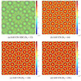
Figure 5: The real morphologies which describe the difference between the numerical solutions and the reference value at $t=0.4025$. The reference solution is obtained by the SDC/CN+SDC method in the case of $N_{T}=2048$. The model parameters are set as $q_{1}=1$, $q_{2}=2\cos(\pi/12)$, $\tilde{\varepsilon}=-2$ and $\tilde{\alpha}=2$.

4.3 The influence of multiple length-scales potential

In this subsection, we use the dodecagonal quasiperiodic phases as an example to investigate the influence of multi-length-scale potentials on the stability of aperiodic structures. Concretely, we consider three, four, and five multiple length scale iPFC models. The parameters in the potential function are set as $q_{j}=s^{j-1}$, $s=2\cos(\pi/12)$, $j=1,\cdots,m$, $m=3,4,5$. The other model parameters are $\tilde{\varepsilon}=-2$ and $\tilde{\alpha}=2$. In the PM, the $\mathcal{P}$ and $\mathbf{B}$ are consistent with Subsec. 4.2. The spatial functions are also discretized in $4$-dimensional space with $24^{4}$ basis functions. The SAV/CN approach with $N_{T}=256$ is adopted to simulate the dynamic process. Fig. 6 lists the corresponding energy evolution plots, initial values, and stationary states. The first row presents the energy evolutions of DDQCs with different length-scale potentials. The second and third rows give the spectral distributions and real morphologies of the $m$-length-scale DDQCs, respectively. The last row shows the real morphologies of stationary solutions. From these results, one can see that the three- and four-length-scale potentials both result in 6-fold symmetric periodic crystal, while the five-length-scale potential can obtain the 12-fold symmetric quasicrystals. Therefore increasing the number of characteristic length-scales in the iPFC model is helpful to stabilize the quasicrystals.

Figure 6: The energy evolutions, initial values and convergence solutions of $m$-length-scale DDQCs under the model parameters $\tilde{\varepsilon}=-2$, $\tilde{\alpha}=2$. The scale parameters are set as $q_{j}=s^{j-1}$, $j=1,\cdots,m$, $s=2\cos(\pi/12)$.

5 Summary

For the iPFC model, we proposed a second-order SAV/CN scheme which is unconditionally energy stable in the almost periodic function sense and gave the error estimate. Meanwhile, we used the SDC approach to further improve the accuracy of the second-order scheme to the fourth-order method through a one-step correction. The PM was applied to discretize spatial functions for computing aperiodic structures to high accuracy. In numerical simulations, the efficiency of the numerical schemes was demonstrated via the numerical convergence rates and the comparison of the dynamic evolutions. By comparing the dynamic evolutions of the DDQCs with different length-scales, we found that increasing the number of characteristic length-scales in the iPFC model significantly is helpful to stabilize aperiodic structures.

References

• [1] [10.1103/PhysRevLett.54.1517] P. Bak, \doititlePhenomenological theory of icosahedral incommensurate (β€œquasiperiodic”) order in Mn-Al alloys, Phys. Rev. Lett., 54 (1985), 1517–1519.
• [2] C. Corduneanu, Almost Periodic Functions, 2nd edition, Chelsea Publishing Company, New York, 1989.
• [3] (MR16068) [10.1215/S0012-7094-46-01311-7] H. Davenport and K. Mahler, \doititleSimultaneous Diophantine approximation, Duke Math. J., 13 (1946), 105–111.
• [4] (MR1765736) [10.1023/A:1022338906936] A. Dutt, L. Greengard and V. Rokhlin, \doititleSpectral deferred correction methods for ordinary differential equations, BIT Numer. Math., 40 (2000), 241–266.
• [5] (MR3919909) [10.4208/cicp.OA-2018-0034] R. Guo and Y. Xu, \doititleSemi-implicit spectral deferred correction method based on the invariant energy quadratization approach for phase field problems, Commun. Comput. Phys., 26 (2019), 87–113.
• [6] M. V. JariΔ‡, Long-range icosahedral orientational order and quasicrystals. Phys. Rev. Lett., 55 (1985), 607–610.
• [7] [10.1080/14786435.2019.1671997] K. Jiang and W. Si, \doititleStability of three-dimensional icosahedral quasicrystals in multi-component systems, Philos. Mag., 100 (2020), 84–109.
• [8] K. Jiang, J. Tong, P. Zhang and A.-C. Shi, Stability of two-dimensional soft quasicrystals in systems with two length scales, Phys. Rev. E, 92 (2015), 042159.
• [9] (MR3117417) [10.1016/j.jcp.2013.08.034] K. Jiang and P. Zhang, \doititleNumerical methods for quasicrystals, J. Comput. Phys., 256 (2014), 428–440.
• [10] [10.1088/1361-648X/aa586b] K. Jiang, P. Zhang and A.-C. Shi, \doititleStability of icosahedral quasicrystals in a simple model with two-length scales, J. Phys.: Condens. Matter, 29 (2017), 124003.
• [11] [10.1007/s10444-020-09789-9] X. Li and J. Shen, \doititleStability and error estimates of the SAV Fourier-spectral method for the phase field crystal equation, Advances in Computational Mathematics, \arXiv1907.07462, 46 (2020), Article number: 48.
• [12] [10.1080/14786430701358673] R. Lifshitz and H. Diamant, \doititleSoft quasicrystals–Why are they stable?, Philos. Mag., 87 (2007), 3021–3030.
• [13] [10.1103/PhysRevLett.79.1261] R. Lifshitz and D. M. Petrich, \doititleTheoretical model for Faraday waves with multiple-frequency forcing, Phys. Rev. Lett., 79 (1997), 1261–1264.
• [14] [10.1107/S2052252518001161] S. Savitz, M. Babadi and R. Lifshitz, \doititleMultiple-scale structures: From Faraday waves to soft-matter quasicrystals, IUCrJ, 5 (2018), 247–268.
• [15] (MR3723659) [10.1016/j.jcp.2017.10.021] J. Shen, J. Xu and J. Yang, \doititleThe scalar auxiliary variable (SAV) approach for gradient flows, J. Comput. Phys., 353 (2018), 407–416.
• [16] (MR2679727) [10.3934/dcds.2010.28.1669] J. Shen and X. Yang, \doititleNumerical approximations of Allen-Cahn and Cahn-Hilliard equations, Discrete Contin. Dyn. Syst., 28 (2010), 1669–1691.
• [17] (MR2519603) [10.1137/080738143] S. M. Wise, C. Wang and J. S. Lowengrub, \doititleAn energy-stable and convergent finite-difference scheme for the phase field crystal equation, SIAM J. Numer. Anal., 47 (2009), 2269–2288.
• [18] (MR3564340) [10.1016/j.jcp.2016.09.029] X. Yang, \doititleLinear, first and second-order, unconditionally energy stable numerical schemes for the phase field model of homopolymer blends, J. Comput. Phys., 327 (2016), 294–316.