Assessing Cosmic Acceleration with the Alcock-Paczyński Effect in the SDSS-IV Quasar Catalog

Abstract

The geometry of the Universe may be probed using the Alcock-Paczyński (AP) effect, in which the observed redshift size of a spherical distribution of sources relative to its angular size varies according to the assumed cosmological model. Past applications of this effect have been limited, however, by a paucity of suitable sources and mitigating astrophysical factors, such as internal redshift-space distortions and poorly known source evolution. In this Letter, we introduce a new test based on the AP effect that avoids the use of spatially bound systems, relying instead on sub-samples of quasars at redshifts $z\lesssim 1.5$ in the Sloan Digital Sky Survey IV, with a possible extension to higher redshifts and improved precision when this catalog is expanded by upcoming surveys. We here use this method to probe the redshift-dependent expansion rate in three pertinent Friedmann-Lemaître-Robertson-Walker (FLRW) cosmologies: $\Lambda$CDM, which predicts a transition from deceleration to acceleration at $z\sim 0.7$; Einstein-de Sitter, in which the Universe is always decelerating; and the $R_{\rm h}=ct$ universe, which expands at a constant rate. $\Lambda$CDM is consistent with these data, but $R_{\rm h}=ct$ is favoured overall.

1 Introduction

The expansion history of the Universe has been probed using a diverse set of observations, including those of the Cosmic Microwave Background Radiation (CMB) and the large-scale structure of galaxy clusters. These approaches have been limited by processes other than those in the baseline cosmological model, however, due to possible source evolution in the latter, or the generation and modification of anisotropies in the former (Narlikar et al., 2007; Angus & Diaferio, 2011; López-Corredoira, 2013; Melia, 2014; López-Corredoira, 2007). Though large surveys of galaxies may constrain the geometry of the Universe, e.g., via the construction of a Hubble diagram or the implementation of an angular-size test, one must typically adopt specific astrophysical models, such as the growth of dark-matter halos, in order to extract useful cosmological information.

The geometry of the Universe can be assessed more cleanly via the Alcock-Paczyński (AP) (Alcock & Paczynski, 1979; López-Corredoira, 2014) effect, in which the ratio of observed radial/redshift size to angular size of a spherical distribution of sources, such as a galaxy cluster, changes from one cosmology to the next. AP tests largely avoid contamination from source evolution because the characteristics of individual sources do not impact the ratio of projected sizes of their distribution. Of course, to fully utilize the AP effect, one must have access to bound systems that are large enough to be measurable over a broad range of redshifts, and this tends to be a principal mitigating factor.

In this Letter, we introduce a new test based on the AP effect designed to probe the cosmic expansion rate as a function of redshift, though using the very large sample of quasars in the Sloan Digital Sky Survey IV (SDSS-IV) (Ahumada et al., 2019), spanning redshifts $z\lesssim 3.5$. The novel feature with this approach is that it does not rely on spatially confined source distributions. As we shall see, the use of quasars can greatly improve the statistics for the purpose of model selection, especially when future surveys will grow this catalog by two or more orders of magnitude.

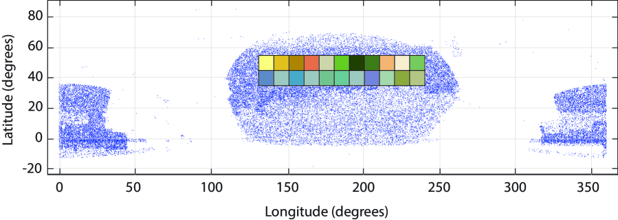
Figure 1: Sky map in Galactic coordinates $(l,b)$, of the projected locations (blue dots) of the 526,356 SDSS-IV quasars. The colored boxes show sub-samples selected for the new AP test (see text). For example, the yellow box has a size of $10^{\circ}\times 10^{\circ}$ and is centered at Galactic coordinates $(135^{\circ},55^{\circ})$.

Our modified AP test can be used for any cosmology but, given our focus on the impact of acceleration on the geometry, we shall here restrict our attention to three highly pertinent models: Planck-$\Lambda$CDM (Planck Collaboration et al., 2018), which predicts different epochs of acceleration and deceleration; Einstein-de Sitter, which has been strongly ruled out as a viable model of the Universe by many other kinds of data, but is included because it provides a well-known example of a Universe that only decelerates; and another FLRW cosmology based on the zero active mass equation-of-state, $\rho+3p=0$, in terms of the total energy density $\rho$ and pressure $p$ in the cosmic fluid (Melia, 2007, 2016, 2017; Melia & Shevchuk, 2012; Melia, 2020). Known as the $R_{\rm h}=ct$ universe, this cosmology exhibits a constant rate of expansion throughtout its history. (See Table 2 in ref. Melia 2018 for a more detailed comparison of this model with $\Lambda$CDM.)

2 Data and Methodology

All of the data we use in this Letter are taken from the Data Release 16 Quasar catalog (DR16Q), based on the extended Baryon Oscillation Spectroscopic Survey (eBOSS) of the SDSS-IV (Ahumada et al., 2019). This collection includes all SDSS-IV/eBOSS objects spectroscopically confirmed as quasars. With the inclusion of previously confirmed quasars from SDSS-I, II and III, this combined catalog encompasses an overall sample of 526,356 objects, though possibly subject to an estimated contamination of about $0.5\%$. This compilation spans a redshift range up to $\sim 3.5$, covering approximatey 9376 deg² of the sky (see fig. 1). As we shall see, however, the quasar number density per comoving volume decreases non-negligibly at $z\gtrsim 1$ (see fig. 3), and we shall therefore restrict our attention to sources below this redshift for this first application of the AP test. In addition, the quasar sample is less complete at low latitudes (i.e., $b\lesssim 30^{\circ}$) compared to $b\gtrsim 30^{\circ}$, due in part to galactic foreground effects. As such, we shall here restrict our analysis to the sub-samples shown as colored boxes in figure 1 to maximize the statistics.

Our methodology utilizes the geometric construction shown in figure 2. In short, we select two adjacent comoving boxes, each with its four lateral sides inclined at a fixed angle $\Delta\theta/2$ (in both galactic latitude $b$ and longitude $l$), relative to the line-of-sight (LOS). We then count the total number of quasars, $N_{Q1}$, in box 1, based on its pre-selected length, $\Delta z_{1}$, in redshift space (more on this below), and find from the quasar catalog the value of $\Delta z_{2}$ for which $N_{Q2}=N_{Q1}$. For a fixed angular size $\Delta\theta\times\Delta\theta$, the redshift interval $\Delta z_{2}$ is a unique function of $\Delta z_{1}$ and the redshift-dependent comoving distance predicted by each given cosmology. A comparison of the ‘measured’ and theoretical relations between $\Delta z_{1}$ and $\Delta z_{2}$ then provides a likelihood of that being the correct model.

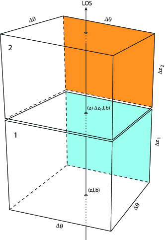
Figure 2: Schematic diagram showing two adjacent boxes along the line of sight (LOS), each with angular dimensions $\Delta\theta\times\Delta\theta$ in the plane of the sky. Box 1 has its base centered at $(z,l,b)$, and has a length $\Delta z_{1}$ in redshift space. Box 2, whose base is centered at $(z+\Delta z_{1},l,b)$, has the corresponding length $\Delta z_{2}$.

In order for this method to provide a meaningful comparison, however, several conditions need to be satisfied. Box 1 has its base centered at coordinates $(z,l,b)$, with an angular size $\Delta\theta\times\Delta\theta$ in the plane of the sky. For convenience, we predict from the chosen cosmological model the redshift size, $\Delta z_{1}$—or, equivalently, the angle $\Delta\theta$—such that all three dimensions, which we shall call $L_{\parallel}(z)$ (in the radial direction) and $L_{\perp}(z)$ (in the two transverse directions at the base), are all equal in the comoving frame. As it turns out, the angular size $L_{\perp}(z)$ does not appear in the final analysis because $\Delta\theta$ remains constant throughout the region $(z,z+\Delta z_{1}+\Delta z_{2})$. $L_{\perp}(z)$ serves only to establish the area at the base of the first box, but because $\Delta\theta$ remains constant, changing $L_{\perp}$ represents a change in its area that is mirrored in proportion by the area of the second box. Thus, the ratio $\Delta z_{2}/\Delta z_{1}$ is independent of $L_{\perp}(z)$, as one may see more formally in the derived condition shown in Equation (13) below. Choosing $\Delta\theta$ in this fashion (if $\Delta z_{1}$ is fixed) merey provides a convenient sub-sample of quasars with which to calculate $N_{Q1}$ and $N_{Q2}$, and may be used for all the cosmologies being tested.

We make the key assumption that the average quasar comoving number density, $n_{Q}(z)$, within the two boxes is uniform on a scale of several degrees. The average density is more likely to be uniform across the boxes as their size increases, of course, though redshift evolution in $n_{Q}(z)$ could invalidate this approach if $dn_{Q}/dz$ from Box 1 to Box 2 is too large to ignore. Any potential evolution in $n_{Q}$ may therefore be mitigated by choosing as small a box as possible, in order to minimize the ratio $(dn_{Q}/dz)\Delta z/n_{Q}$. Unfortunately, these two requirements conflict each other, but we have found by direct inspection of the SDSS-IV catalog that any dispersion arising from these effects is well within the final calculated errors as long as $\Delta z_{1}/z\lesssim 1/3$ and $z\lesssim 1$. One may see this graphically in figure 3, which shows the estimated DR16Q quasar number density per unit comoving volume, assuming Planck-$\Lambda$CDM as the background cosmology (see Eqns. 5 and 6 below). (Note that this plot is merely used to gauge how reliable our assumption of a constant $n_{Q}$ is, and is not included in the comparative analysis, which needs to be carried out independently for each individual cosmology.) Evidently, $n_{Q}$ is very nearly constant up to $z\sim 1.2$, and then decreases monotonically towards higher redshifts.

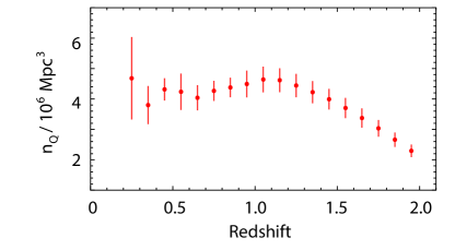
Figure 3: The DR16Q quasar number density as a function of redshift, assuming Planck-$\Lambda$CDM as the background cosmology (see Eqns. 5 and 6).

Of the three cosmologies we shall test here, the geometry in $R_{\rm h}=ct$ is the easiest to understand because all of its integrated measures—such as the comoving distance—have simple analytical forms. We shall therefore start with this model, and then summarize the corresponding expressions for the other two. For Box 1 along the LOS, we have in the $R_{\rm h}=ct$ universe

$$L^{R_{\rm h}}_{\parallel}(z)={c\over H_{0}}\int_{z}^{z+\Delta z_{1}}{du\over E(u)}\;,$$ (1)

where $H(z)\equiv H_{0}E(z)$, $E(z)=(1+z)$ and $H_{0}$ is the Hubble constant. For our actual calculations, we shall employ the full integral expressions for these quantities. It will also be helpful, however, for us to understand the results by finding approximations in the limit where $\Delta z\ll z$. In this limit, Equation (1) may be written

$$L^{R_{\rm h}}_{\parallel}(z)\approx{c\Delta z_{1}\over H_{0}(1+z)}\,.$$ (2)

In the plane of the sky, the corresponding comoving size is

$$L^{R_{\rm h}}_{\perp}(z)\approx\Delta\theta{c\over H_{0}}\ln(1+z)\;.$$ (3)

Thus, to estimate a reasonable size $\Delta z_{1}$ for Box 1 when $\Delta\theta$ is chosen, or $\Delta\theta$ if $\Delta z_{1}$ is fixed, we may simply set these two expressions equal to each other, $L^{R_{\rm h}}_{\parallel}(z)=L^{R_{\rm h}}_{\perp}(z)$, and find that

$$\Delta z_{1}\approx\Delta\theta(1+z)\ln(1+z)\;.$$ (4)

For $\Lambda$CDM, the corresponding quantities are

$$L^{\Lambda}_{\parallel}(z)={c\over H_{0}}\int_{z}^{z+\Delta z_{1}}{du\over\sqrt{\Omega_{\rm m}(1+z)^{3}+\Omega_{\Lambda}}}\;,$$ (5)

and

$$L^{\Lambda}_{\perp}(z)=\Delta\theta{c\over H_{0}}\int_{0}^{z}{du\over\sqrt{\Omega_{\rm m}(1+u)^{3}+\Omega_{\Lambda}}}\;.$$ (6)

In these expressions, $\Omega_{\rm m}$ and $\Omega_{\Lambda}$ are today’s matter and dark-energy densities, respectively, scaled to the critical density $\rho_{\rm c}\equiv 3c^{2}H_{0}^{2}/8\pi G$. Radiation may be ignored for $z\lesssim 3.5$. The parametrization shown in Equations (5) and (6) is based on the Planck optimization (Planck Collaboration et al., 2018): $\Omega_{\rm m}=0.315\pm 0.007$, $\Omega_{\Lambda}=1.0-\Omega_{\rm m}$ (given that $\Omega_{k}=0.001\pm 0.002$ is fully consistent with a perfectly flat Universe), and an equation-of-state parameter $w_{\rm de}=-1.03\pm 0.03$, where the pressure of dark energy is written as $p_{\rm de}=w_{\rm de}\rho_{\rm de}$, in terms of its corresponding energy density $\rho_{\rm de}$. This points to a cosmological constant, for which $p_{\rm de}=-\rho_{\rm de}$. In our analysis, we shall therefore assume flat $\Lambda$CDM with $w_{\rm de}=-1$, though we shall allow $\Omega_{\rm m}$ to vary in order to optimize the fit. This procedure is independent of all other parameters, such as $H_{0}$. Finally, in the case of Einstein-de Sitter, we have

$$L^{\rm EdS}_{\parallel}(z)\approx{c\Delta z_{1}\over H_{0}(1+z)^{3/2}}$$ (7)

and

$$L^{\rm EdS}_{\perp}(z)=\Delta\theta{2c\over H_{0}}\left(1-{1\over\sqrt{1+z}}\right)\,,$$ (8)

which together yield

$$\Delta z_{1}\approx 2\Delta\theta(1+z)\left(\sqrt{1+z}-1\right)\,.$$ (9)

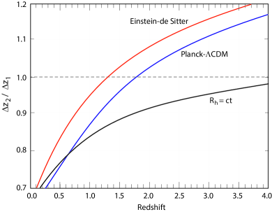
Figure 4: The ratio $\Delta z_{2}/\Delta z_{1}$ as a function of $z$, assuming $\Delta z_{1}=z/3$: (blue) Planck-$\Lambda$CDM; (black) the $R_{\rm h}=ct$ universe; and (red) Einstein-de Sitter. The standard model transitions from acceleration to deceleration across $z\sim 0.7$, while Einstein-de Sitter always decelerates, and $R_{\rm h}=ct$ expands at a constant rate.

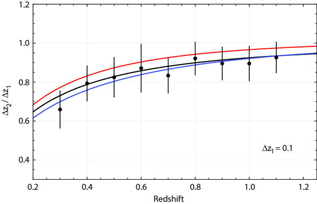
Figure 5: Same as figure 4, except now for a fixed $\Delta z_{1}=0.1$, highlighting the variation with redshift at $0\lesssim z\lesssim 1.2$. The color coding is the same as in figure 4, except that blue now corresponds to the best-fit $\Lambda$CDM model, with the optimized matter density $\Omega_{\rm m}=0.22^{+0.21}_{-0.10}$. The data points are obtained by counting quasars in the DR16Q catalog.

Were we to ignore the $\delta z$-dependence of $L_{\perp}(z+\delta z)$ over the redshift range $\delta z\in(0,\Delta z_{1})$ and $(\Delta z_{1},\Delta z_{1}+\Delta z_{2})$, the comoving volumes 1 and 2 would be equal if $\Delta z_{2}$ were chosen to satisfy the condition

$$\int_{z+\Delta z_{1}}^{z+\Delta z_{1}+\Delta z_{2}}{du\over E(z)}=\int_{z}^{z+\Delta z_{1}}{du\over E(z)}\;.$$ (10)

This is not a good approximation, however, even for boxes with $\Delta z_{1}/z\lesssim 1/3$. Fortunately, it is quite straightforward to incorporate the redshift-dependence of $L_{\perp}$ into a calculation of the comoving volume, via the inclusion of the expression

$$L_{\perp}(z+\delta z)=L_{\parallel}(z)\left[1+{I(z,z+\delta z)\over I(0,z)}\right]\;,$$ (11)

where

$$I(z_{1},z_{2})\equiv\int_{z_{1}}^{z_{2}}{du\over E(u)}\;.$$ (12)

Since $\Delta\theta$ remains constant across both boxes, it is not difficult to see that $\Delta z_{2}$ must satisfy the condition

$$I(0,z+\Delta z_{1}+\Delta z_{2})^{3}=2I(0,z+\Delta z_{1})^{3}-I(0,z)^{3}\;.$$ (13)

The complete solution for $\Delta z_{2}/\Delta z_{1}$, taking all of these spherical effects into account, is shown in figure 4 for each of the three cosmologies, using the criterion $\Delta z_{1}=z/3$. We show in this figure the expected model differences over the extended range ($0\lesssim z\lesssim 4$), principally to demonstrate the importance of conducting this test at high redshifts using the expanded quasar catalog that will be assembled with upcoming surveys. Given the limitations of DR16Q (see fig. 3), however, we shall be focusing our attention on the more restricted range ($0\lesssim z\lesssim 1$) in this paper (see fig. 5), as an illustration of the method.

It has been noted elsewhere (see, e.g., refs. Melia 2018, 2020) that the transition from deceleration to acceleration at $z\sim 0.7$ in $\Lambda$CDM produces an overall expansion history very similar to that of $R_{\rm h}=ct$, at least up to $z\sim 1$. The two phases effectively cancel out, producing an integrated expansion approximately equal to what it would have been if the Universe had expanded at a constant rate from the beginning. This is reflected in the overlap between the two $\Delta z_{2}/\Delta z_{1}$ (black and blue) curves below $z\sim 1$ in figure 4. At higher redshifts ($z\gtrsim 1.5$), however, the cosmological constant in Equations (5) and (6) becomes relatively unimportant, and $\Lambda$CDM exhibits the effects of deceleration analogous to Einstein-de Sitter.

To differentiate between cosmological models with different combinations of unknowns, one typically uses information criteria, such as the Akaike Information Criterion, ${\rm AIC}\equiv\chi^{2}+2f$, where $f$ is the number of free parameters (Akaike, 1974; Liddle, 2007; Burnham & Anderson, 2002; Melia & Maier, 2013), and the Kullback Information Criterion, ${\rm KIC}\equiv\chi^{2}+3f$ (Cavanaugh, 2004). A third variant, known as the Bayes Information Criterion (Schwarz 1978), is defined as ${\rm BIC}=\chi^{2}+f\ln N$, where $N$ is the number of data points. The BIC is actually not based on information theory, but rather on an asymptotic ($N\rightarrow\infty$) approximation to the outcome of a conventional Bayesian inference procedure for deciding between models. It suppresses overfitting much more than AIC and KIC if $N$ is large. In the application we are considering here, $N\lesssim 30$, for which $\ln(30)\sim 3.4$, compared to the analogous factor $2$ in the case of AIC, and $3$ for KIC. In this case, the BIC does not provide a perspective very different from the other two criteria, and there is no point in including it in this Letter.

For model $\mathcal{M}_{\alpha}$, the unnormalized confidence of it being ‘true’ is the Akaike weight $\exp(-{\rm AIC}_{\alpha}/2)$. Thus, its relative likelihood of being the correct choice is

$$P(\mathcal{M}_{\alpha})=\frac{\exp(-{\rm AIC}_{\alpha}/2)}{\sum_{\beta}\exp(-{\rm AIC}_{\beta}/2)}\;.$$ (14)

The various outcomes may also be characterized via the difference $\Delta{\rm AIC}\equiv{\rm AIC}_{2}\nobreak-{\rm AIC}_{1}$ (and similarly for KIC), which determines the extent to which $\mathcal{M}_{1}$ is favoured over $\mathcal{M}_{2}$. The result is judged ‘positive’ when $\Delta\sim 2-6$, ‘strong’ for $\Delta\sim 6-10$, and ‘very strong’ if $\Delta\gtrsim 10$.

3 Results and Discussion

A direct comparison of these three curves with the ‘measurement’ of $\Delta z_{2}/\Delta z_{1}$ using quasar counts in the DR16Q catalog is shown in figure 5. The errors associated with measuring the position of each quasar, $(z,l,b)$, are insignificant compared to the dispersion in their comoving number density $n_{Q}$. To estimate the errors shown here, we therefore assemble as many boxes as possible within the same redshift bin $\Delta z_{1}$ (though clearly not at the same angular position), and then calculate the population variance from this distribution. The error bars shown in figure 5 represent the $1\sigma$ uncertainties inferred from this variance.

Table 1: Model Selection using AP with the SDSS-IV quasar catalog

Model	$\chi^{2}$	AIC	Prob	KIC	Prob
			(AIC)		(KIC)
$R_{\rm h}=ct$	$1.094$	$1.095$	$62.4\%$	$1.095$	$69.6\%$
$\Lambda$CDM ($\Omega_{\rm m}=0.22^{+0.21}_{-0.10}$)	$0.827$	$2.827$	$26.3\%$	$3.827$	$17.8\%$
Einstein-de Sitter	$4.513$	$4.513$	$11.3\%$	$4.513$	$12.6\%$

The fits in this plot, and the summary of results given in Table 1, show that the data are consistent with $\Lambda$CDM, but actually somewhat favour the $R_{\rm h}=ct$ cosmology, which expands at a constant rate at all redshifts, while strongly rejecting Einstein-de Sitter. The optimized matter density $\Omega_{\rm m}=0.22^{+0.21}_{-0.10}$ for $\Lambda$CDM is fully consistent with the Planck measurement (i.e., $0.315\pm 0.007$). In a head-to-head comparison, the result that $R_{\rm h}=ct$ is favoured over $\Lambda$CDM is judged positive, with an outcome $\Delta{\rm AIC}\sim 1.7$ and $\Delta{\rm KIC}\sim 2.7$, based on the DR16Q catalog.

Unlike many other kinds of observation, these data are effectively independent of any model because they are constrained by a fixed $\Delta\theta$ throughout the redshift range $(z,z+\Delta z_{1})$ and $(z+\Delta z_{1},z+\Delta z_{1}+\Delta z_{2})$, and they do not depend on the actual value of $L_{\perp}(z)$. Thus, the same set of data apply to all three curves in figure 5. For a fixed $\Delta\theta$, however, the ratio $L_{\parallel}(z)/L_{\perp}(z)$ of the boxes does change in redshift space according to each model’s prediction of the angular diameter distance. As we may see from this figure, the statistical weight of the DR16Q quasar catalog is already sufficient for us to start distinguishing between the three models we have examined in this paper.

But clearly, the probative power of this technique will grow considerably when future surveys will allow us to extend this test to redshifts as high as $\sim 3.5$ (see fig. 4). Upcoming campaigns will expand the quasar catalog by several orders of magnitude. For example, projections for the Large Synoptic Survey Telescope (Izevic, 2017) imply that perhaps as many as 50 million detections will have been confirmed over the lifetime of this collaboration, enhancing the current DR16Q catalog a hundredfold. With such improved statistics, one may even model $n_{Q}(z)$ individually for each cosmology over redshifts where the comoving density is not constant (see fig. 3), thereby attaining an even higher level of precision for the $\Delta z_{2}/\Delta z_{1}$ curves.

Data Availability Statement

All of the data underlying this paper are taken from the Data Release 14 Quasar catalog (DR16Q), based on the extended Baryon Oscillation Spectroscopic Survey (eBOSS) of the SDSS-IV, which is fully described in Ahumada et al. (2019). The DR16Q catalog may be downloaded in fits format from the website https://www.sdss.org/dr16/.

References

- Ahumada et al. (2019) Ahumada, R., Allende Prieto, C., Almeida, A., et al. 2019, arXiv e-prints, arXiv:1912.02905
- Akaike (1974) Akaike, H. 1974, IEEE Transactions on Automatic Control, 19, 716
- Alcock & Paczynski (1979) Alcock, C., & Paczynski, B. 1979, Nat, 281, 358
- Angus & Diaferio (2011) Angus, G. W., & Diaferio, A. 2011, MNRAS, 417, 941
- Burnham & Anderson (2002) Burnham, K. P., & Anderson, D. R. 2002, Model Selection and Multimodel Inference (Springer-Verlag)
- Cavanaugh (2004) Cavanaugh, J. E. 2004, Aust N Z J Stat, 46, 257
- Izevic (2017) Izevic, Z. 2017, Proceedings of the International Astronomical Union, IAU Symposium, 324, 330
- Liddle (2007) Liddle, A. R. 2007, MNRAS, 377, L74
- López-Corredoira (2007) López-Corredoira, M. 2007, Journal of Astrophysics and Astronomy, 28, 101
- López-Corredoira (2013) —. 2013, International Journal of Modern Physics D, 22, 1350032
- López-Corredoira (2014) —. 2014, ApJ, 781, 96
- Melia (2007) Melia, F. 2007, MNRAS, 382, 1917
- Melia (2014) —. 2014, A&A, 561, A80
- Melia (2016) —. 2016, Frontiers of Physics, 11, 119801
- Melia (2017) —. 2017, Frontiers of Physics, 12, 129802
- Melia (2018) —. 2018, MNRAS, 481, 4855
- Melia (2020) —. 2020, The Cosmic Spacetime (Taylor & Francis)
- Melia & Maier (2013) Melia, F., & Maier, R. S. 2013, MNRAS, 432, 2669
- Melia & Shevchuk (2012) Melia, F., & Shevchuk, A. S. H. 2012, MNRAS, 419, 2579
- Narlikar et al. (2007) Narlikar, J. V., Burbidge, G., & Vishwakarma, R. G. 2007, Journal of Astrophysics and Astronomy, 28, 67
- Planck Collaboration et al. (2018) Planck Collaboration, Aghanim, N., Akrami, Y., et al. 2018, arXiv e-prints, arXiv:1807.06209
- Schwarz (1978) Schwarz, G. 1978, Annals of Statistics, 6, 461