agtboost: Adaptive and Automatic Gradient Tree Boosting Computations

Berent Lunde, Tore Kleppe agtboost: Adaptive and Automatic Gradient Boosting Computations agtboost: Automatic Function Estimation agtboost is an R package implementing fast gradient tree boosting computations in a manner similar to other established frameworks such as xgboost and LightGBM, but with significant decreases in computation time and required mathematical and technical knowledge. The package automatically takes care of split/no-split decisions and selects the number of trees in the gradient tree boosting ensemble, i.e., agtboost adapts the complexity of the ensemble automatically to the information in the data. All of this is done during a single training run, which is made possible by utilizing developments in information theory for tree algorithms (Lunde et al., 2020). agtboost also comes with a feature importance function that eliminates the common practice of inserting noise features. Further, a useful model validation function performs the Kolmogorov-Smirnov test on the learned distribution. gradient tree boosting, information criterion, automatic function estimation, R gradient tree boosting, information criterion, automatic function estimation, R Berent Ånund Strømnes Lunde
Department of Mathematics and Physics
Faculty of Science and Technology
University of Stavanger
Kristine Bonnevies vei 22
4021 Stavanger, Norway
E-mail:

1 Introduction: Tuning of gradient tree boosting

Gradient tree boosting (GTB) (Friedman, 2001; Mason et al., 1999) has risen to prominence for regression problems after the introduction of xgboost (Chen and Guestrin, 2016). The GTB model is an ensemble-type model, that consist of classification and regression trees (CART) (Breiman et al., 1984) that are learned in an iterative manner. GTB models are very flexible in that they automatically learn non-linear relationships and interaction effects. However, with the increased flexibility of GTB models comes substantial worries of overfitting. The top performing gradient tree boosting libraries, such as xgboost, LightGBM (Ke et al., 2017) and catboost (Dorogush et al., 2018), all come with a large number of hyperparameters available for manual tuning to constrain the complexity of the GTB models. Training of gradient tree boosting models, in general, thus require some familiarity with both the chosen package, and the data for efficient tuning and application to the problem at hand.

The main focus of the hyperparameters and tuning are to solve the following problems:

• The complexity of trees: What are the topology of all the different trees? Too complex trees overfits, while simple stump-models cannot capture interaction effects. This is typically solved using a hyperparameter that penalizes (equally) the number of leaves in the tree. xgboost hyperparameters for this are gamma, max_depth, min_child_weight, and max_leaves.

• The number of trees: How many iterations should the tree-boosting algorithm do before terminating? Too early stopping will leave information unlearned, while too late stopping will see the last trees adapting mostly to noise. An early-stopping hyperparameter is usually tuned to obtain ensembles of adequate size. Tuned in xgboost with nrounds.

• Making space for feature trees to learn: If each tree is optimized alone, early trees will have a tendency to learn additive relationships and information that subsequent trees could learn more efficiently (Friedman et al., 2000). An additional downside of large early trees is difficult model-interpretability. The hyperparameter solution typically involves tuning the maximum depth (max_depth in xgboost) globally for all trees.

The five parameters of xgboost mentioned above are typically selected as the top-performing parameters found from $k$-fold cross validation (CV) (Stone, 1974). CV, however, increases computation times extensively, and requires more work through coding and knowledge on the part of the user.

agtboost is an implementation of the theory in Lunde et al. (2020), which unlocks computationally fast and automatic solutions to the problems listed above, and as a consequence removes selection of hyperparameters through CV from the problem. The key is an information criterion that can be applied after the greedy binary-splitting profiling procedure used in learning trees. The theory is built upon maximal selection of chi-squared statistics (White, 1982; Gombay and Horvath, 1990) and the convergence of an empirical process to a continuous time stochastic process. Lunde et al. (2020) subsequently discuss how both tree-size and the number of trees then can be chosen automatically. This paper supplements Lunde et al. (2020) by describing a package built on this theory, i.e., agtboost. Some new innovations are also introduced, which all have their basis in the information criterion. In general, they address the problems with feature importance and the optimization of trees alone.

Note that there exist other hyperparameters that may increase accuracy (but that are not vital) for GTB models. Most notably are parameters for a regularized objective (see e.g., Chen and Guestrin (2016)) and stochastic sampling of observations during boosting iterations (for an overview, see Hastie et al. (2001) and for recent innovations for GTB see Ke et al. (2017)). These features are not yet implemented, but subject to further research, as more work is required to adhere to the philosophy of agtboost – that all hyperparameters should be automatically tuned.

This paper starts by introducing gradient tree boosting in Section 2 and the information criterion in Section 3, and proceeds with the innovations and software implementation in Section 4. Section 5 describes agtboost from a user’s perspective. Section 6 studies and compares the different variants of agtboost models for the large sized Higgs dataset. Finally, Section 7 discusses and concludes.

2 Gradient tree boosting

This and the following section closely follow the setup of Lunde et al. (2020). The (typical) objective of gradient tree boosting procedures is the supervised learning problem

$$f(x)=\arg\min_{f}E[l(y,f(x))],$$ (1)

for a response $y\in R$, feature vector $x\in R^{m}$, and loss function $l$ measuring the difference between the response and prediction $\hat{y}=f(x)$. For gradient boosting to work, we require $l$ to be both differentiable and convex. Then, using training data, say $\mathcal{D}_{n}=\{(y_{i},x_{i})\}_{i=1}^{n}$, we seek to approximate (1) by learning $f$ in an iterative manner: Given a function $f^{(k-1)}$, we seek $f_{k}$ to minimize

$$f_{k}(x)=\arg\min_{f_{k}}E[l(y,f^{(k-1)}(x)+f_{k}(x))],$$ (2)

approximately to second order. This is done by computing the derivatives

$$g_{i,k}=\left.\frac{\partial}{\partial\hat{y}^{(k-1)}}l(y,\hat{y}^{(k-1)})\right|_{\hat{y}^{(k-1)}=f^{(k-1)}(x)},\leavevmode\nobreak\ h_{i,k}=\left.\frac{\partial^{2}}{\partial(\hat{y}^{(k-1)})^{2}}l(y,\hat{y}^{(k-1)})\right|_{\hat{y}^{(k-1)}=f^{(k-1)}(x)},$$ (3)

for each observation in the training data, and then approximate the expected loss by averaging,

$$f_{k}(x)=\arg\min_{f}\frac{1}{n}\sum_{i=1}^{n}l(y,\hat{y}_{i}^{(k-1)})+g_{i,k}f_{k}(x)+\frac{1}{2}h_{i,k}f_{k}(x)^{2}.$$ (4)

Terminating this procedure at iteration $K$, the final model is an additive model of the form

$$\hat{y}_{i}=\hat{y}^{(K)}=\sum_{k=1}^{K}f_{k}(x_{i}).$$ (5)

Still, (4) is a hard problem, as the search among all possible functions is obviously infeasible. Therefore, it is necessary to constrain the search over a a family of functions, or "base learners". While multiple choices exist, agtboost follows the convention of using CART (Breiman et al., 1984).

For a full discussion of decision trees, see (Hastie et al., 2001) for a general treatment, and Lunde et al. (2020) for details on its use in gradient tree boosting and agtboost. We constrain ourselves to a brief mention of important aspects. Firstly, decision trees learn constant predictions (called leaf-weights) in regions of feature space. We let $I_{t,k}=\{i:q_{k}(x)=t\}$ denote the index-set of training indices that falls into region (or leaf) $t$, denoted by $q_{k}(x)=t$, where $q_{k}$ is the topology of the $k$’th tree, a function that takes the feature vector and returns the the node-index or corresponding index of region in feature space, $t$. The prediction from the tree is given by

$$f_{k}(x_{i})=w_{q_{k}(x_{i})}.$$ (6)

Secondly, the estimated leaf-weights have closed form in the 2’nd order boosting procedure described above, namely

$$\hat{w}_{t,k}=-\frac{G_{t,k}}{H_{t,k}}\>\text{where}\>G_{t,k}=\sum_{i\in I_{t,k}}g_{i,k}\>\text{and}\>H_{t,k}=\sum_{i\in I_{t,k}}h_{i,k}.$$ (7)

Thirdly, the regions of feature space are learned by iteratively splitting all leaf-regions (starting with the full feature space as the only leaf) creating new leaves and regions. The region is split on the split-point that gives the largest reduction in training loss, say $R_{t}$, among all possible binary splits. This search is fast, as the training loss, modulus unimportant constant terms, in region $t$ is given as

$$l_{t}=-\frac{G_{t,k}^{2}}{2nH_{t,k}},$$ (8)

and enumeration of possible splits can therefore be done in $mn\log n$ time.

The above procedure creates the decision tree $f_{k}$, which is then added to the model $f^{(k-1)}$ by

$$f^{(k)}=f^{(k-1)}+\delta f_{k},\leavevmode\nobreak\ \delta\in(0,1).$$ (9)

The constant $\delta$, typically called the "learning rate" or "shrinkage", leaves space for feature models to learn. Values are often taken as "small", but this comes at the added computational cost of an increase in the number of boosting iterations (infinite when $\delta\to 0$) before convergence. The learning rate is the only hyperparameter of the boosting procedure in agtboost that is not tuned automatically. The default value is set at $0.01$, which should be sufficiently small for most applications without incurring too much computational cost.

3 Information criteria

This section introduces generalization loss-based information criteria, which includes types such as Akaike Information Criterion (AIC) (Akaike, 1974), Takeuchi Information Criterion (TIC) (Takeuchi, 1976) and Network Information Criterion (NIC) (Murata et al., 1994). Generalization loss is perhaps better known as an instance of test loss, say $l(y^{0},f(x^{0}))$, where $(y^{0},x^{0})$ is an observation unseen in the training phase, i.e., not an element and independent of $\mathcal{D}_{n}$. This specification is important, as (1) is intended for this quantity, and using the training loss, in our case (4) as an estimator, care must be taken as the training loss is biased downwards in expectation. This bias is known as the optimism of the training loss (Hastie et al., 2001), and denoted $C$. A generalization loss-based information criterion, say $\tilde{C}$, is intended to capture the size of the optimism, such that adding $\tilde{C}$ to the training loss gives an (at least approximately) unbiased estimator of the expected generalization loss.

The equation behind the generalization loss-based information criteria mentioned above is

$$\tilde{C} =\texttt{tr}\left(E\left[\nabla_{\theta}^{2}l\left(y,f(x;\theta_{0})\right)\right]Cov(\hat{\theta})\right),$$ (10)

$$\tilde{C} \approx E[l(y^{0},f(x^{0};\hat{\theta}))]-E[l(y_{1},f(x_{1};\hat{\theta}))],$$

where $(y_{1},x_{1})$ is a (random) instance of the training dataset, and $\theta_{0}$ is the population minimizer of (1) where optimization is done over a parametric family of functions and $\hat{\theta}$ is not at the boundary of parameter space (Burnham and Anderson, 2003, Eqn. 7.32).

In the GTB training procedure described in section 2, the model selection questions of added complexity are always at the "local" root (constant prediction) versus stump (a tree with two leaf-nodes) model. It is always one, and only one, node at a time that is tried split in this gradient tree boosting procedure. Thus isolate this relevant node by assuming and conditioning on that $q(x)=t$, then node $t$ may be referenced and treated as a root. Further, for convenient notation, assume to be at some boosting iteration $k$, thus dropping notational dependence on current iteration, and let $l$ and $r$ denote the left and right child nodes of node $t$. The idea of Lunde et al. (2020) is to use the optimism of the root (node $t$, conditioned on data falling into leaf $t$, i.e., $q(x)=t$) and stump model (split of node $t$, with the same conditioning as for the root), say $C_{\text{root}}$ and $C_{\text{stump}}$, to adjust the root and stump training loss, to see if there is expected a positive reduction in generalization loss,

$$-\frac{1}{2n}\left[\frac{G_{t}^{2}}{H_{t}}-\left(\frac{G_{l}^{2}}{H_{l}}+\frac{G_{r}^{2}}{H_{r}}\right)\right]+C_{\text{root}}-C_{\text{stump}}>0,$$ (11)

which would be used to decide if to split further in a tree, and to see if a tree-stump model $f_{k}$ could be added to the ensemble $f^{k-1}$. The root and stump training loss combined in the parenthesis is the loss-reduction, $R$, that is profiled over for different binary splits. This profiling, however, complicates evaluation of the above inequality as it induces optimism into $C_{stump}$ which (10) cannot handle directly.

We may combine the root and stump optimisms to create a loss-reduction optimism, say $C_{R}=C_{\text{root}}-C_{\text{stump}}$. Lunde et al. (2020) derives the following estimator for the optimism of loss-reduction

$$\tilde{C}_{R}=-\tilde{C}_{root}\pi_{t}E\left[B(\mathbf{x})\right],$$ (12)

where $\pi_{t}$ is the probability of being in node $t$, estimated by the fraction of training data passed to node $t$, and $\tilde{C}_{root}$ is calculated as (10) conditioned on being in node $t$, and may be estimated using the sandwich estimator (Huber et al., 1967) together with the empirical Hessian. The remaining quantity in (12), $B(\mathbf{x})$ where $\mathbf{x}$ is the full design matrix of the training data, is a maximally chosen random variable

$$B(\mathbf{x})=\max_{j\leq 1\leq m}B_{j}(x_{\cdot j}),\leavevmode\nobreak\ B_{j}(x_{\cdot j})=\max_{1\leq k\leq a}S_{j}(\tau_{k})$$ (13)

defined from a specification of the Cox-Ingersoll-Ross process (CIR) (Cox et al., 1985), $S(\tau)$, with speed of adjustment to the mean $2$, long term mean $1$ and instantaneous rate of volatility $2\sqrt{2}$, therefore having dynamics given by the SDE

$$dS(\tau)=2(1-S(\tau))dt+2\sqrt{2S(\tau)}dW(\tau),$$ (14)

which is "observed" at time-points $\tau_{k}=\frac{1}{2}\log\frac{u_{k}(1-\epsilon)}{\epsilon(1-u_{k})},\>\epsilon\to 0$ defined from the split-points $u_{k}=p(x_{ij}\leq s_{k})$, $i=1:(n-1)$ on feature $j$. To estimate $E[B(\mathbf{x})]$ is, however, not straight forward. Lunde et al. (2020) discuss a solution using exact simulation of the CIR process using $\epsilon=10^{-7}$, together with the fact that the stationary CIR is in the maximum domain of attraction of the Gumbel distribution (Gombay and Horvath, 1990), an independence assumption on features, and numerical integration to evaluate the expectation.

4 Software implementation and innovations

agtboost employs the r.h.s. of (12) to solve the list of problems presented in the introduction, which for other implementations are solved by tuning the hyperparameters using techniques such as cross-validation (CV) (Stone, 1974). The use of (12) alleviates the need for hyperparameters tuned with CV, as it allows the base-learner trees $f_{k}$ and the ensemble $f^{(k)}$ to stop at a given complexity that is adapted to the training data at hand. Thus significantly increasing the speed of training a gradient tree boosting ensemble. Furthermore, the technical knowledge imposed on the user, with respect to both gradient tree boosting and the dataset at hand, is reduced. agtboost is coded in C++ for fast computations, and relies on Eigen (Guennebaud et al., 2010) for linear algebra, the R header files (R Core Team, 2018) for some distributions, and Rcpp (Eddelbuettel and François, 2011) for bindings to R. The remainder of this section goes through the innovations in agtboost that directly attacks the previously mentioned tuning-problems.

4.1 Adaptive tree size

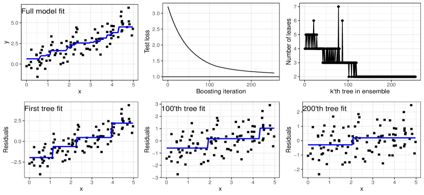
Figure 1: Top: [left] Full model fit on training-data, [middle] test loss versus the number of boosting iterations, with the minimum expected loss possible (true model) included with a horizontal line, and [right] the number of leaves in the $k$’th tree. Bottom: The First, 100’th and 200’th tree fits to the training MSE-residuals, $r_{i}^{(k)}=-g_{i,k}/h_{i,k}=y_{i}-\hat{y}^{(k-1)}$ at respective iterations. The $n=100$ training and test observations were i.i.d. generated with a linear structural relationship and Gaussian noise, $x\sim U(0,5)$ and $y\sim N(x,1)$.

Equipped with an information criterion for loss reduction after greedy-split-profiling, the necessary adjustments are rather straight-forward, and are also discussed in Lunde et al. (2020). For completeness, the usage of (12) towards selecting the complexity of trees $f_{k}$ is restated here: After the split that maximizes training loss reduction $R$ is found, the following inequality is tested

$$R+\tilde{C}_{R}>0,$$ (15)

and if it evaluates to TRUE, then two new leaves (and regions) are created and successive splitting on them is performed. This continues until (15) evaluates to FALSE. This criterion is employed for all but the first (root) split, which is forced. This forced split is done to assure some increase in model complexity, as $\sum_{i}g_{i}=0$ is always true and a root model will therefore be equivalent to adding zero to the model.

Figure 1 illustrates this adaptivity: Visually, it is seen that trees assign higher leaf-node predictions to observations with high values of $x$ than to small values of $x$, thus capturing the structural relationship $y=x$ in the simulated data. Furthermore, of the trees plotted in the lower lane together with residuals $y_{i}-\hat{y}_{i}^{(k-1)}=-g_{i,k}/h_{i,k}$ at iterations $k\in\{1,100,200\}$, none of them can be seen to be complex enough to adapt to the Gaussian noise in the training data. Indeed, every subsequent iteration reduces the value of test loss, seen from the top-middle panel. Further verification of this is given by the decreasing complexity of trees (measured in terms of number of leaves), corresponding to residuals at early iterations necessarily containing more information than later ones. Thus, early trees therefore tend to be more complex than at later stages of the training.

4.2 Automatic early stopping

The natural stopping criterion for the iterative boosting procedure, in the context of supervised learning, is to stop when the increase in model complexity no longer gives a reduction in generalization loss. From Figure 1, the top-right plot shows that the later iterations tend to be tree-stumps. Indeed, a tree constructed using the method described in Section 4.1 will be a tree stump at the iteration where the natural stopping criterion terminates the algorithm. This is because a more complex tree must have passed the "barrier" (i.e., inequality) (15), and necessarily will have a decrease in generalization loss, as long as $\delta\in(0,1]$. Care must however be taken, as we are scaling the $k$’th tree with the learning rate, $\delta$, and 15 might therefore not be used directly. Lunde et al. (2020) discuss this: The solution lies in the general equation for Equation (10) (Hastie et al., 2001)

$$\tilde{C}=\frac{2}{n}\sum_{i=1}^{n}Cov(y_{i},\hat{y}_{i}),$$ (16)

and the optimism therefore scales linearly. The training loss, on the other hand, does not and can be seen to scale with the factor $\delta(2-\delta)$ from direct computations. Scaling the training loss and optimism appropriately, agtboost evaluates a similar inequality as (15), namely

$$\delta(2-\delta)R+\delta\tilde{C}_{R}>0,$$ (17)

which if evaluates to FALSE, indicates that the increased complexity does not decrease generalization loss, and subsequently the boosting procedure is terminated.

The top-left panel of Figure 1 illustrates the fit of a model that converged after $K=255$ iterations, and also shows a "convergence plot" (top-middle panel with test loss at different boosting iterations) that flattens out. Indeed, repetitions of the same experiment with an increased number of training instances, $n$ (see top row of Figure 2), shows that the test loss converges on average towards 1, indicated by the horizontal line. This is the expected minimum value possible due to the standard Gaussian noise. Furthermore, if considering the lower-right plot with the fit of the 200’th tree to the residuals at that iteration, we can see that the algorithm still finds information that is hard to see for the naked eye. The algorithm continues for another 55 iterations, that still manages to decrease test loss.

4.3 The global-subset algorithm

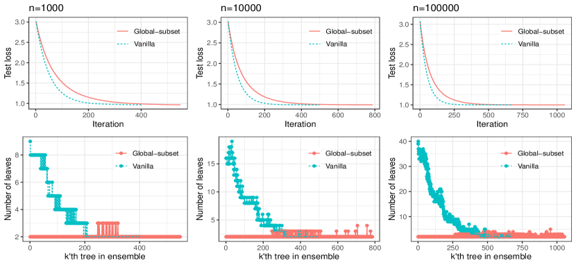
Figure 2: Top: Test loss at different boosting iterations for the global-subset and vanilla algorithms training and testing with an increasing number of observations. Lower: The number of leaves in the $k$’th tree for the global-subset and vanilla algorithms, also training and testing with the same number of observations as in the top row. The data generating process is the same as described in the caption of Figure 1, but with the number of training and test observations set to $n=\{1000,10000,100000\}$ for the three columns.

Equipped with the information criterion (12), it is possible to construct a solution to the problem that each tree is optimized alone, mentioned as the third point in the introduction. For this subsection, denote the reduction in training loss from splitting some node $t$ at the $k$’th boosting iteration by ${}_{k}R_{t}$. For example, the reduction from the root-node split at the same $k$’th iteration is denoted ${}_{k}R_{1}$ and the reduction from splitting the root-node at the $(k+1)$’th boosting iteration is denoted ${}_{k+1}R_{1}$.

The idea is rather simple, namely to compare the average generalization loss reduction from a chosen split in the $k$’th boosting iteration, with that of the average generalization loss reduction we would obtain from the root-split in the $(k+1)$’th boosting iteration if the aforementioned split was not performed and the recursive splitting at the $k$’th iteration terminated. This then allows the tree-boosting algorithm to consider (in a greedy manner) all possible allowed changes in function complexity of the ensemble, not just a deeper tree. The naive approach to do this – at each possible split in the $k$’th iteration, temporarily terminate, and start on the $(k+1)$’th iteration for inspection of the root-split reduction in generalization loss – is computationally infeasible. Instead, notice that, as $\delta\to 0$, the 2’nd order gradient boosting approximation to the loss is increasingly accurate, and that, at the limit $\delta\to 0$, we have $f_{k}=f_{k+1}$, as $f_{k}$ is scaled to zero by the learning rate. Necessarily, we have ${}_{k}R_{1}\approx{}_{k+1}R_{1}$ and $\tilde{C}_{{}_{k}R_{1}}\approx\tilde{C}_{{}_{k+1}R_{1}}$.

The quantities ${}_{k+1}R_{1}$ and $\tilde{C}_{{}_{k+1}R_{1}}$ may be used to adjust the right-hand-side of (15) with the expected reduction in generalization loss of the next split, so that the recursive binary splitting terminates when splitting the next root-node is more beneficial. Using ${}_{k}R_{1}$ and $\tilde{C}_{{}_{k}R_{1}}$ as replacements, the reformulated split-stopping inequality yields

$$\pi_{t}^{-1}\left({}_{k}R_{t}+\tilde{C}_{{}_{k}R_{t}}\right)>\max\left\{0,{}_{k}R_{1}+\tilde{C}_{{}_{k}R_{1}}\right\}.$$ (18)

The probability $\pi_{t}$ is introduced to adjust for the difference in the number of training observations, as the root works on the full dataset, while node $t$ necessarily works on some subset of the data. The inequality (18) is then employed as a replacement for- and in the exact same manner as (15)

Figure 2 illustrates the practical difference in pathological learning behaviour: The data exhibits purely additive behaviour. Friedman et al. (2000) argues for a model consisting only of tree-stumps in this case. Both method converges to a test loss of approximately 1, the minimum expected test loss possible for a perfect model, for all values of $n$. The difference lies in the complexity and number of trees. The vanilla algorithm (using (15)) builds each tree as if it was the last, and already at the first iteration, several regions of feature space will be split into sub-regions, seen from the plots in the lower row. The global-subset algorithm, however, "looks ahead" and often evaluates that terminating the recursive binary splitting procedure and starting on a new boosting iteration is more beneficial. Subsequently, trees are rarely complex and thus easier to interpret, but comes to the cost of a higher number of boosting iterations before terminating by the inequality (17). This cost is decreased, however, as boosting iterations are overall faster than for the vanilla algorithm since individual trees are less complex.

5 Using the agtboost package

The goal of the agtboost package is to avoid expert opinions and computationally costly brute force methods with regards to tuning the functional complexity of GTB models. Usage should be as simple as possible. As such, the package has only two main functions, gbt.train for training an agtboost model, and a predict function that overloads the predict function in R. The main responsibility of the user is to identify a "natural" loss-function and link-function. To this end, agtboost also comes with a model validation function, gbt.ksval, which performs a Kolmogorov-Smirnov test on supplied data, and a function for feature importance, gbt.importance, that functions similarly to ordinary feature importance functions (see for instance Hastie et al. (2001)) but which calculates reduction in loss with respect to (approximate) generalization loss and not the ordinary training loss. Due to implementation using Rcpp modules, saving and loading of agtboost cannot be done by the ordinary save and load functions in R, but is made possible through the functions gbt.save and gbt.load. Table 1 gives an overview of the implemented loss functions in agtboost.

Type	Distribution	Link	Comment
mse	Gaussian	$\mu=f(x)$	Ordinary regression for continuous response
logloss	Bernoulli	$\log\left(\frac{\mu}{1-\mu}\right)=f(x)$	Regression for classification problems
gamma::neginv	Gamma	$-\frac{1}{\mu}=f(x)$	Gamma regression for positive continuous response
gamma::log	Gamma	$\log(\mu)=f(x)$	regression for positive continuous response
poisson	Poisson	$\log(\mu)=f(x)$	Poisson regression for count data exhibiting $Var(y|x)=E[y|x]$
negbinom	Negative binomial	$\log(\mu)=f(x)$	For count data exhibiting overdispersion. dispersion must be supplied to gbt.train

Table 1: Overview of the loss functions available in agtboost.

Following is a walk-through of the agtboost package, applied to the caravan.train and caravan.test data (Van Der Putten and van Someren, 2000) that comes with the package and documented there. The caravan dataset has a binary response, indicating purchase of caravan insurance, and 85 socio-demographic covariates. Due to the nature of the response, classification using the logloss loss function is natural. To train a GTB model, it is only needed to specify the loss_function argument in gbt.train R> mod <- gbt.train(y = caravan.train$y,x=caravan.train$x, loss_function = "logloss", verbose = 100) it: 1 | n-leaves: 3 | tr loss: 0.2166 | gen loss: 0.2167 it: 100 | n-leaves: 2 | tr loss: 0.1983 | gen loss: 0.2019 it: 200 | n-leaves: 3 | tr loss: 0.1927 | gen loss: 0.1987 it: 300 | n-leaves: 2 | tr loss: 0.1898 | gen loss: 0.1978 Note the verbose=100 argument, which creates output at the first and every 100’th iteration. The output consists of the iteration number, the number of leaves of the $k$’th tree, the training loss and approximate generalization loss. By default, the global-subset algorithm using inequality (18) is used instead of (15), if the latter is preferred, specify algorithm = "vanilla" as an argument to gbt.train.

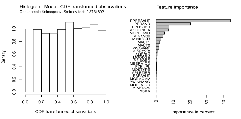
Figure 3: [left] Histogram generated by gbt.ksval, where test-response observations are transformed using (5). As the histogram closely resembles the histogram of standard uniformly distributed random variables, the model should not be discarded, something also indicated by the formal Kolmogorov-Smirnov test. [right] Feature importance plot generated by gbt.importance.

The overloaded predict function may be used to check the fit on the training data, or to predict new data. To predict data, just pass the model object and the design matrix of data to be predicted R> prob_te <- predict(mod, caravan.test$x)Itisoftenmeaningfultodosomeformalgoodness-of-fittestinadditiontoonlyvisuallyinspectingthefit.Aquitenaturalandgeneralwaytodothisforlossfunctionsassociatednegativelog-likelihoods,istousetheKolmogorov-Smirnovtest\cite[citep]{(\@@bibref{AuthorsPhrase1Year}{kolmogorov1933sulla}{\@@citephrase{, }}{})}.Theideaisto,foracontinuousresponse,performtheCDFtransform\begin{aligned} u_{i}=p\left(y\leq y_{i};\hat{\theta}(x_{i})\right),\end{aligned}preferablyfortest-data,andtestthe$u_i${}^{\prime}sagainstthestandarduniformdistribution,whichholdsifthemodeliscorrectlyspecified.Iftheresponseisdiscrete,thenemploythetransform\begin{aligned} u_{i}=p\left(y\leq y_{i}-1;\hat{\theta}(x_{i})\right)+Vp\left(y_{i};\hat{\theta}(x_{i})\right),\end{aligned}where$V∼U(0,1)$,insteadoftheCDFtransform.Allofthisisimplementedinthe\code{gbt.ksval}function.Toapplyittothecaravandatamodel,simplywrite\CodeChunk\CodeInput R>gbt.ksval(object=mod,y=caravan.test$y,x=caravan.test$x)\CodeOutput ClassificationOne-sampleKolmogorov-Smirnovtestdata:uD=0.021877,p-value=0.3732alternativehypothesis:two-sidedwhichproducesoutputofthetest-statistic,thep-valueandthehistograminFigure\ref{fig:using_agtboost_caravan}.Notethatformulti-parameterdistributions,suchastheGaussian,gammaandnegativebinomial,theremainingparametersareassumedconstantandmaximum-likelihoodestimatesareproducedduringevaluationofthe\code{gbt.ksval}functiontoallowforthetransforms\eqref{eq:continous-uniform-transform}and\eqref{eq:discrete-uniform-transform}.Theestimateswillthenbeproducedintheoutput.\par Inadditiontothe\code{gbt.ksval}function,the\code{gbt.importance}functioncanbeusedtoinspectthemodel.Thisfunctionproducesatraditionalfeatureimportanceplot(seee.g.\cite[citet]{\@@bibref{Authors Phrase1YearPhrase2}{friedman2001elements}{\@@citephrase{(}}{\@@citephrase{, Chap.\leavevmode\nobreak\ 15.3.2)}}}),butdifferentfromotherpackages,thecalculationsarewithrespecttoapproximategeneralizationloss.Formally,fornon-leafnodes$t$inalltreesintheensemble,thevalue\begin{aligned} \delta(2-\delta)R_{t}+\delta\tilde{C}_{R_{t}}\end{aligned}isaddedtothe$j$-thelementofavector,where$j$isthe$j$-thfeatureusedforthesplit.Thewayinwhich\code{gbt.importance}calculatesimportance,andduetothesparsemodelsproducedby\code{gbt.train},know-howtrickssuchasinsertingGaussiannoise-featuresarenotnecessarywhenusing\pkg{agtboost}.TherightplotinFigure\ref{fig:using_agtboost_caravan}producesthefeatureimportanceplotforthecaravanmodel.Notethatonly24of85possiblefeaturesareusedbythemodel.Re-trainingthemodelwithonlytheserelevantfeaturesmightimprovethefit,asthe61featuresnotusedbythemodelarenoisethatmaskinformationandenlargestheabsolutevalueoftheinformationcriterion\eqref{eq:information-criteria-loss-reduction}.\par\par\par$

6 Higgs big-data case study

The two variants of agtboost is tested across increasing training sizes of a dataset, and their intrinsic behaviour with regards to reduction in loss, number of trees and leaves of trees, numbers of features used, and convergence across boosting iterations is studied. We refer to models using inequality (15) as "vanilla" models, and models using the global-subset algorithm (18) as "global-subset" models. To this end, the Higgs dataset is used. The Higgs data consists of 11 million observations of a binary response and 28 continuous features. The first 10 million observations are used for training, and the last million for testing for which results are reported. The training set is sampled randomly without replacement for $n=\{10^{2},10^{3},10^{4},10^{5}\}$ observations, and trained on the respective training indices. Tests and reported results are always done on the one-million sized test-set.

Algorithm	Loss	AUC	Time	#trees	#leaves	#features
$n=100$
vanilla	0.6728	0.5942	0.1417	32	64	1
global-subset	0.6734	0.5942	0.1386	30	60	1
$n=1000$
vanilla	0.6483	0.703	2.335	162	422	7
global-subset	0.6437	0.7071	1.623	184	504	8
$n=10000$
vanilla	0.5692	0.7796	1.191	684	4976	22
global-subset	0.5708	0.7781	1.201	768	4008	18
$n=100000$
vanilla	0.5317	0.8087	32.57	1055	43908	28
global-subset	0.5321	0.8085	34.17	1176	29105	28

Table 2: Results of the two algorithms available in agtboost for different number of training samples available. The Loss (Logloss) and AUC is computed on the test set with 1 million observations. The remaining columns are the total number of trees in the models, the total number of leaves summed up over all trees, and the total number of features used by the models. Loss metrics and computation times are almost identical, while complexity and construction differs.

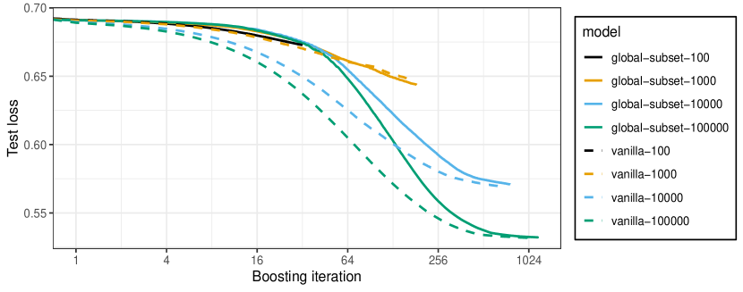
Figure 4: Test loss as a function of boosting iterations, for the vanilla and global-subset models trained on $n\in\{100,1000,10000,100000\}$ training observations. More training observations imply more information, which allow for lower points of convergence and a greater number of boosting iterations. The methods stop at different boosting iterations. Notice the log scale on the horizontal axis.

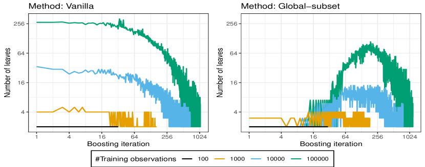
Figure 5: The number of leaves for the $k$’th tree (boosting iteration $k$) for different agtboost models trained on the Higgs data with a varying number of training observations. Notice the log scale on both the vertical and horizontal axes.

In the "Loss" column of Table 2 it is seen that the test-loss is decreasing in the size of the training set, as it should. Figure 4 compliments this result: Each model is seen to converge and values of test loss flatten out as a function of boosting iterations. But, as the training set increases, more information in the data is present that allow lower points of convergence. None of the models are seen to overfit in the number of boosting iterations, as the curves never increase.

While the two variants of agtboost converge to similar results in terms of test-loss, and the methods take a similar amount of time (column 5 of Table 2), their behaviour during training and the complexity of the resulting models differ. Figure 5 shows two different ways of learning the structural signal in the data. The early trees of the vanilla algorithm start with deep trees, and as the signal is learned, trees become smaller. Trees from the global-subset algorithm, on the other hand, start out with mere tree stumps, and then increase in size as interaction effects become more beneficial to learn than additive relationships. Trees do however not reach the depth of the deepest early trees of the vanilla algorithm. As interaction effects are taken into the model, these trees also become smaller before convergence of the boosting algorithm. The total number of trees and leaves of the models are shown in columns 6 and 7 in Table 2. While the global-subset algorithm produces models with a larger number of trees than the vanilla algorithm, the total number of leaves is typically smaller, but without a loss of accuracy. As sparsity is a good defence against the curse of dimensionality, the performance of the global-subset algorithm might become more evident on big-$p$ small-$n$ datasets.

7 Discussion

This paper describes agtboost, an R package for gradient tree boosting solving regression-type problems in an automated manner. The package takes advantage of recent innovations in information theory with regards to the splits in gradient boosted trees Lunde et al. (2020), implements these in C++ for fast computation and employs RcppEigen for bindings to R which provides user-friendly application. The package comes with two different utilizations of the information criterion (12), that vary little in final accuracy and in training time but vary in terms for individual tree-size and complexity. The package can be used for early exploratory data analysis for selecting features and an appropriate loss-function, but also for building a final highly predictive model.

References

- Akaike (1974) Akaike H (1974). “A New Look at the Statistical Model Identification.” IEEE Transactions on Automatic Control, 19(6), 716–723.
- Breiman et al. (1984) Breiman L, Friedman J, Stone CJ, Olshen RA (1984). Classification and Regression Trees. CRC Press.
- Burnham and Anderson (2003) Burnham KP, Anderson DR (2003). Model Selection and Multimodel Inference: A Practical Information-Theoretic Approach. Springer Science & Business Media.
- Chen and Guestrin (2016) Chen T, Guestrin C (2016). “XGBoost: A Scalable Tree Boosting System.” In Proceedings of the 22nd acm sigkdd international conference on knowledge discovery and data mining, pp. 785–794.
- Cox et al. (1985) Cox JC, Ingersoll JE, Ross SA (1985). “A Theory of the Term Structure of Interest Rates.” Econometrica, 53(2), 385–407.
- Dorogush et al. (2018) Dorogush AV, Ershov V, Gulin A (2018). “CatBoost: Gradient Boosting with Categorical Features Support.” arXiv preprint arXiv:1810.11363.
- Eddelbuettel and François (2011) Eddelbuettel D, François R (2011). “Rcpp: Seamless R and C++ Integration.” Journal of Statistical Software, 40(8), 1–18. 10.18637/jss.v040.i08. URL http://www.jstatsoft.org/v40/i08/.
- Friedman et al. (2000) Friedman J, Hastie T, Tibshirani R, et al. (2000). “Additive Logistic Regression: A Statistical View of Boosting (With Discussion and a Rejoinder by the Authors).” The Annals of Statistics, 28(2), 337–407.
- Friedman (2001) Friedman JH (2001). “Greedy Function Approximation: a Gradient Boosting Machine.” Annals of Statistics, pp. 1189–1232.
- Gombay and Horvath (1990) Gombay E, Horvath L (1990). “Asymptotic Distributions of Maximum Likelihood Tests for Change in the Mean.” Biometrika, 77(2), 411–414.
- Guennebaud et al. (2010) Guennebaud G, Jacob B, et al. (2010). “Eigen v3.” http://eigen.tuxfamily.org.
- Hastie et al. (2001) Hastie T, Tibshirani R, Friedman J (2001). The Elements of Statistical Learning. Springer Series in Statistics New York, NY, USA:.
- Huber et al. (1967) Huber PJ, et al. (1967). “The behavior of maximum likelihood estimates under nonstandard conditions.” In Proceedings of the fifth Berkeley symposium on mathematical statistics and probability, volume 1, pp. 221–233. University of California Press.
- Ke et al. (2017) Ke G, Meng Q, Finley T, Wang T, Chen W, Ma W, Ye Q, Liu TY (2017). “LightGBM: A Highly Efficient Gradient Boosting Decision Tree.” In Advances in Neural Information Processing Systems, pp. 3146–3154.
- Kolmogorov (1933) Kolmogorov A (1933). “Sulla determinazione empirica di una lgge di distribuzione.” Inst. Ital. Attuari, Giorn., 4, 83–91.
- Lunde et al. (2020) Lunde BÅS, Kleppe TS, Skaug HJ (2020). “An information criterion for automatic gradient tree boosting.” arXiv preprint arXiv:2008.05926.
- Mason et al. (1999) Mason L, Baxter J, Bartlett P, Frean M (1999). “Boosting Algorithms as Gradient Descent in Function Space (Technical Report).” RSISE, Australian National University.
- Murata et al. (1994) Murata N, Yoshizawa S, Amari Si (1994). “Network Information Criterion-Determining the Number of Hidden Units for an Artificial Neural Network Model.” IEEE Transactions on Neural Networks, 5(6), 865–872.
- R Core Team (2018) R Core Team (2018). R: A Language and Environment for Statistical Computing. R Foundation for Statistical Computing, Vienna, Austria. URL https://www.R-project.org/.
- Stone (1974) Stone M (1974). “Cross-Validatory Choice and Assessment of Statistical Predictions.” Journal of the Royal Statistical Society. Series B (Methodological), pp. 111–147.
- Takeuchi (1976) Takeuchi K (1976). “Distribution of Information Statistics and Validity Criteria of Models.” Mathematical Science, 153, 12–18.
- Van Der Putten and van Someren (2000) Van Der Putten P, van Someren M (2000). “CoIL challenge 2000: The insurance company case.” Technical report, Technical Report 2000–09, Leiden Institute of Advanced Computer Science ….
- White (1982) White H (1982). “Maximum likelihood estimation of misspecified models.” Econometrica: Journal of the Econometric Society, pp. 1–25.