Vol.0 (20xx) No.0, 000–000
\vs\noReceived 20xx month day; accepted 20xx month day
A WISE View of IRAS Debris Disks: Revising the Dust Properties
Abstract
Debris disks around stars are considered as components of planetary systems. Constrain the dust properties of these disks can give crucial information to formation and evolution of planetary systems. As an all-sky survey, InfRared Astronomical Satellite (IRAS) gave great contribution to the debris disk searching which discovered the first debris disk host star (Vega). The IRAS-detected debris disk sample published by Rhee (Rhee et al. 2007) contains 146 stars with detailed information of dust properties. While the dust properties of 45 of them still can not be determined due to the limitations with the IRAS database (have IRAS detection at 60 m only). Therefore, using more sensitivity data of Wide-field Infrared Survey Explorer (WISE), we can better characterize the sample stars: For the stars with IRAS detection at 60 m only, we refit the excessive flux densities and obtain the dust temperatures and fractional luminosities; While for the remaining stars with multi-bands IRAS detections, the dust properties are revised which show that the dust temperatures were over estimated in high temperatures band before. Moreover, we identify 17 stars with excesses at the WISE 22 m which have smaller distribution of distance from Earth and higher fractional luminosities than the other stars without mid-infrared excess emission. Among them, 15 stars can be found in previous works.
keywords:
(stars:) circumstellar matter — protoplanetary disks —infrared: stars1 Introduction
Debris disks are almost dust-dominated and surround their stars with a wide age range (Hughes et al. 2018). The dust is usually not primordial because its lifetime was much shorter than the stellar age (Wyatt 2018). Debris disks are considered as planetary systems components or protoplanetary disks descendants, which provides a wealth of valuable information on evolution of circumstellar disks and planet formation outcome (Wyatt et al. 2017).
Since IRAS first discovered Vega with debris disk in 1984 (Auman et al. 1984), attempts of searching debris disk candidates are never stop. The most effective way of searching debris disk is to detect the infrared (IR) excess with IR radiation exceeds the stellar photospheric radiation The dust surrounds the sample stars and reaches a thermal equilibrium under stellar radiation, then it will re-emits the light absorbed from the host star at IR to sub-millimeter (Krivov 2010).
Up to now, many hundreds of debris disks have been discovered (Wyatt 2018). They are based on five satellites as follows: IRAS (Rhee et al. 2007; Mannings & Barlow 1998), Infrared Space Observatory (ISO) (Oudmaijer et al. 1992; Kessler et al. 1996; Abraham et al. 1999; Fajardo et al. 1999; Habing et al. 1999; Spangler et al. 2001; Decin et al. 2003), Spitzer (Chen et al. 2005; Rieke et al. 2005; Kim et al. 2005; Su et al 2006; Beichman et al. 2006; Moór et al. 2006; Bryden et al. 2006; Siegler et al. 2007; Rebull et al. 2008; Moór et al. 2011; Wu et al. 2012; Chen et al. 2014; Mittal et al. 2015; Ballering et al. 2018), Herschel (Matthews et al. 2010; Eiroa et al. 2013; Dodson-Robinson et al. 2016; Vican et al. 2016; Sibthorpe et al. 2018) , and AKARI (Fujiwara et al. 2013; Liu et al. 2014; Ishihara et al. 2017). Among these surveys, IRAS and AKARI are all-sky surveys and the other three (Spitzer, ISO and Herschel) are not. Though with much smaller area covering, the latter three missions have much better sensitivities and spatial resolutions so that they can detect more faint disks.
However, IRAS and AKARI still have their own advantages because of their all-sky area. And although both IRAS and AKARI are all-sky surveys, the debris disk candidates detected by them are not exactly the same. The debris disk sample of Rhee (Rhee et al. 2007) detected by IRAS contains 146 stars with debris disk candidates via cross-correlating the IRAS Point Source Catalog (PSC) and Faint Source Catalog (FSC) with the Hipparcos main sequence star catalog. And the debris disk sample of Liu (Liu et al. 2014) detected by AKARI contains 72 stars debris disk candidates via cross-correlating the AKARI/Far-Infrared Surveyor (Kawada et al. 2007) All-Sky Survey Bright Source Catalogue (AKARIBSC, Yamamura et al. 2010) with the Hipparcos main sequence star catalog. Among these two samples, 27 stars are in common although they have the similar sensitivity (IRAS at 60 m band and AKARI/FIS at 90 m). Most of the sources in Rhee’s sample cannot detected by AKARI/FIS because of its shallow limit. So Rhee’s sample still has its own value.
The sample of Rhee gives dust properties of debris disks including dust temperature, fractional luminosity and dust mass. It present a good sample for other works, such as follow up observations of debris disks (Herschel: Marshall et al. 2013; Vican et al. 2016, Spitzer: Chen et al. 2014; Mittal et al. 2015, ALMA: Booth et al. 2019 and Submillimeter: Bulger et al. 2013; Holland et al. 2017); debris disks around A-type stars (Greaves et al. 2016; Welsh & Montgomery 2018; Moór et al. 2017); Individual disk research (Fujiwara et al. 2009; Borgniet et al. 2014; Hung et al. 2015; Su et al. 2015; Konopacky et al. 2016; Geiler et al. 2019). Moreover, this sample focus on debris disks evolution which gives great guidance to evolution works of other people (Wyatt et al. 2007; Moór et al. 2011; Vican & Schneider 2014). And this sample is also helpful to other statistical works: metallicity (Maldonado et al. 2012), binaries (Rodriguez & Zuckerman 2012), Kuiper Belts (Nilsson et al. 2010) and so on.
However, the dust properties of 45 of them still can not be determined due to the limitations with the IRAS database: these stars have only IRAS 60 m detection. This limitation can be broken through with more sensitivity observation data of Wide-field Infrared Survey Explorer (WISE). Many studies have used WISE to search for IR excess stars (Cotten & Song 2016; Wu et al. 2013, 2016). WISE makes an all-sky survey at four IR bands with at 3.4m, at 4.6m, at 12m and at 22 m. The angular resolutions of corresponding bands are 6\farcs1, 6\farcs4, 6\farcs5 & 12\farcsand the 5 point source sensitivities of corresponding bands are better than 0.08, 0.11, 1 and 6 mJy. For high SNR sources, the astrometry precision is better than 0\farcs15 (Wright et al. 2010). The flux densities of and can be used to test the fitting quality of model spectra. And the flux densities of and can be used to fit the dust components and revise the properties.
This paper has refitted the SEDs of Rhee’s sample stars and refitted the excessive flux densities with WISE all-sky source catalog and IRAS catalog to revise the dust properties and get Mid-IR excess information. The sample and photosphere emission are described in Section 2 and results and analysis including the properties of debris disks and hosting stars as well as WISE 22m excess are presented in Section 3. I will discuss the revised dust properties and Mid-IR excess sample in Section 4 and draw the summary in Section 5.
2 The Sample and Photosphere Emission
2.1 The Sample
The sample used in this work is debris disks of 146 stars within 120 pc of Earth detected by IRAS (Rhee et al. 2007), which cross-correlate the IRAS Point Source Catalog (PSC) and Faint Source Catalog (FSC) with the Hipparcos main sequence star catalog. IRAS makes an all-sky survey at four bands centered at 12, 25, 60, and 100 m (Neugebauer et al. 1984). The Hipparcos main sequence star catalog has more than 110,000 stars with the information of photometry and astrometry for the nearby stars (Bessell 2000).
All stars have debris disks around, which are identified by excesses at IRAS 60 m as described in the paper of Rhee. We will check these results in the Section 3. Note that 3 stars were removed from the sample: 2 pre-main-sequence stars (HIP 53911, HIP 77542) and 1 star (HIP 19704) with a detection at 60 m flux quality of 1 (which means the flux quality is not reliable). The sample has 143 stars left over.
2.2 The Photosphere Emission
It is essential to obtaining the 143 sample stars’ photosphere flux densities in order to identify and measure the IR excess strength (Bryden et al. 2006). To construct the SEDs, we collected the optical data ( and from the Hipparcos satellite measurements) to near-infrared (NIR) absolute photometric data ( from Two Micron All Sky Survey (2MASS) catalog) for all sample stars (Skrutskie et al. 2006) and converted these observed magnitudes into flux density (Janskys) by using the zero magnitudes in Cox et al. 2000. The photometry of the sample stars are listed in Table 1. Then we use Kurucz’ models (ATLAS9,Castelli et al. 2004) to fit the stellar SEDs as our previous work do (Liu et al. 2014). The best model was selected out with the minimum which are presented in Table 1.
3 Results and Analysis
With the best-fit Kurucz model, we can estimate the flux densities of stellar photosphere in the corresponding WISE and IRAS bands. We check the IRAS excesses of all 143 sample stars by using the criterion [FIRAS - Fphot] / 3.0, where is the IRAS flux densities; is the predicted photospheric flux densities of corresponding bands; and is the uncertainties of the IRAS flux densities in corresponding bands.
3.1 WISE 22 m Excess
The observation data of WISE will be used to search Mid-IR excess objects. All 143 stars are covered by WISE. While our previous work showed that the model fluxes at WISE 12 and 22 m have the systematical uncertainties with and (Liu et al. 2014). Therefore, the systematical uncertainty should be considered to the uncertainties of WISE all bands with , where means the observational uncertainties of WISE. Note that 3 stars (HIP 70952, HIP 71284, HIP 74946) were removed from the sample with [Fw4obs - Fw4phot] where Fw4obs is the WISE 22 m flux density and Fw4phot is the predicted photospheric flux density at 22 m band. Therefore, there are 140 stars left in our sample for further discussion. These 140 stars’s WISE magnitudes information can be seen from Table 1.
The flux densities of and can be used to test the fitting quality of model spectra. And the flux densities of and can be used to fit the dust components and revise the dust properties of the stars in Rhee et al. (2007). We can estimate the Mid-IR excesses at WISE 22 m in the same way as 60 m excess shown:
[Fw4obs - Fw4phot] / 3.0,
We identify 31 stars with excesses at the 22 m by applying this criterion. While this criterion is affected by the IRAS 100 m background, whose level should be lower than 5 MJy/sr as Kennedy & Wyatt 2012 and Wu et al. 2013 shown. We check the 31 m excess stars and find indeed there are 14 stars may be affected. So there are only 17 stars left after this cut. Mid-IR excess stars are thought to have co-existence of hot and cold dust components just like our solar system. These 17 stars are putted into Mid-IR excess sample which are listed in Table 2. At the following sections, I will discuss this two sub-samples: Mid-IR excess sample and Non Mid-IR excess sample.
3.2 Properties of Debris Disk Host stars
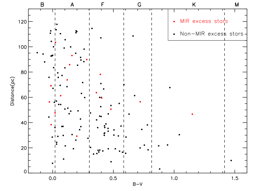
In this subsection, I will study the stellar properties of debris disk hosts including color, distance from the Earth and location on the H-R diagram. Debris disk host stars are more inclined to early type stars as Rhee et al. (2007) pointed out which can be seen from the figure of sample stars function distribution of the distance from Earth and B-V. We re-draw the figure and mark the Mid-IR excess objects in red dots as Figure 1 shown. From the figure, we can see Mid-IR excess sample has smaller distribution of distance from Earth (29.2 pc to 103.5 pc) than Non Mid-IR excess sample stars (3.2 pc to 117.8 pc). Note that there are only 17 Mid-IR excess stars, the sample is so small that may lead to a false distribution trend.
3.3 Dust Properties
In this subsection, I will study the dust properties including the dust temperatures and fractional luminosities of debris disks.
3.3.1 Dust Temperatures
Debris disks usually consist of a single narrow ring which reach thermal equilibrium in the field of stellar radiation as previous studies suggested (Backman & Paresce 1993). Rhee et al. (2007) used the blackbody model with single-temperature to fit the dust component and obtained dust temperature for each star.
Since IRAS sample of Rhee is based on solely IRAS, the dust properties of 45 objects in their sample still can not be determined due to the limitations with the IRAS database (have IRAS detection at 60 m only). They set the dust temperature to 85 K so the peak will fall at 60 m. According to the number of the IRAS detected bands, I divide the 140 stars sample to 2 groups:
(1) Group I contains 45 stars with only IRAS 60 m detection;
(2) Group II contains the remaining 95 stars with multi-bands IRAS detections.
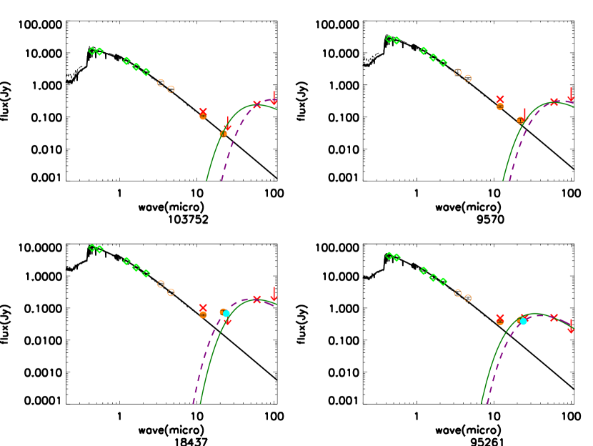
The excessive flux densities are fitted in IR bands including 60, 100 m of IRAS and 12, 22 m of WISE with a blackbody model of single temperature. The SED fittings of 4 stars as an example are presented in Figure 2. From SED fittings, the dust temperatures can be derived with group I stars listed in Table 3 and Group II stars listed in Table 4. From the figure, one can easily see that our fitting results are better than Rhee’s because of the addition of new WISE data.
3.3.2 Fractional Luminosities
From the SED fitting, we can also estimate the fractional luminosity which is used to characterize the disk’s effective optical depth. The fractional luminosity is calculate by divided the IR luminosity of debris disk to the stellar luminosity (Wyatt 2008),
| (1) |
where is the stellar luminosity estimated by the best model of SED fitting. The IR luminosity is calculated from the blackbody model of fitted IR. The calculated fractional luminosities for all sample stars are listed in Table 3 and Table 4 as well.
4 Discussion
In this section, I will first give my discussion on revising the dust properties including dust temperatures and fractional luminosities. And then, I will discuss the Mid-IR excess sample.
4.1 Revising the Dust Temperatures
The revised dust temperature can be seen in Table 3 and Table 4. For Group I stars, we can get the dust temperatures which were set to 85 K in Rhee et al. 2007. And for Group II stars, even they have multi-bands IRAS detections, the dust temperatures of ours are well determined than that in Rhee et al. 2007 because of the much better sensitivity in the Mid-IR of WISE in comparison with IRAS.
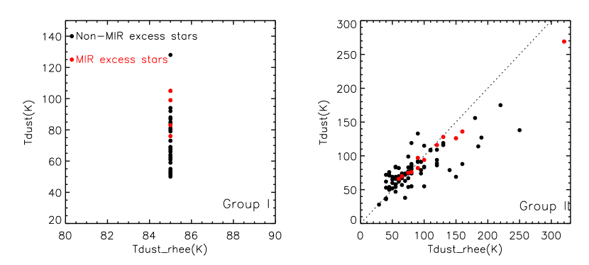
The difference of dust temperatures between Rhee et al. (2007) and ours is shown in Figure 3. From Figure 3, we can see the dust temperatures of Group II stars are over estimated in high temperatures band. While in lower temperature band (100 K), dust temperatures have a part under estimated and a part over estimated, which have no obvious favoritism.
4.2 Revising the Fractional Luminosities
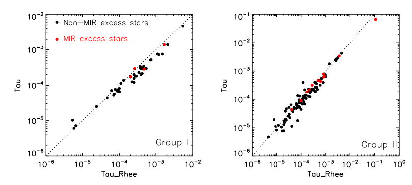
The differences of fractional luminosities between Rhee et al. (2007) and ours are shown in Figure 4. It is obvious that the fractional luminosities of Group I stars are high estimated by Rhee due to the high estimated dust temperatures which can be seen from the left panel of Fig. 4. While for Group II stars, the fractional luminosities show no obvious favoritism with a part under estimated and a part over estimated which can be seen from the right panel of Fig. 4. However, for the Mid-IR excess sample stars in this group, fractional luminosities of mine are almost the same as Rhee et al. (2007). It is most likely because they have plenty of IR excess data to do blackbody fittings.
Whether in Group I or Group II, Mid-IR sample stars have high fractional luminosities than Non Mid-IR sample stars which imply that the stars with higher fractional luminosities may have higher probability of having warm dust component.
4.3 Mid-IR Excess Sample (WISE 22 m)
From Section 3, Mid-IR excess sample contains 17-stars with WISE 22 m excesses. Such stars with Mid-IR excess emission may have terrestrial planets (Padgett & Stapelfeldt 2016).
Up to now, a few hundreds of warm disks with Mid-IR excess have been discovered with Spitzer, AKARI and WISE (Meyer et al. 2008; Fujiwara et al. 2010; Fujiwara & Ishihara et al. 2010; Olofsson et al. 2012; Ribas et al. 2012; Fujiwara et al. 2013; Wu et al. 2012, 2013; Liu et al. 2014; Ishihara et al. 2017; Ballering et al. 2018), and such disks’ incidence decreases very rapidly with increasing stellar ages (Urban et al 2012).
What is the cause of the warm component? For most warm debris disks, the Mid-IR excesses could be explained by giant impact stages (about 100 Myr) (Genda et al. 2015). They found that, after a giant impact, the IR excess is sometimes almost 10 times higher than the stellar IR flux.
In Mid-IR excess sample, 15 stars can be found in previous work as Table 2 column 3 shown. Note \addthat maybe the remaining 2 stars can be seen in the other work elsewhere.
5 Summary
This paper has refitted the SEDs of the sample stars with the Kurucz’ models and refitted the excessive flux densities with WISE and IRAS all sky catalogs. we obtain the dust temperatures of Group I stars with only 60 m data which can not determined in previous study of Rhee. And for Group II stars, even they have IRAS multi-bands detections, the dust temperatures of ours are well determined than that in Rhee et al. 2007 because of the much better sensitivity in the Mid-IR of WISE in comparison with IRAS. From the revised dust properties, we can see that the dust temperatures of Group II stars were over estimated in high temperatures band before and the fractional luminosities of Group I stars were high estimated.
Moreover, we identify 17 stars with WISE 22 m excess and discuss the difference from Non Mid-IR sample. Disks around the Mid-IR sample stars appear to be more bright and with higher dust temperatures. We hope these revision of dust properties can give some guidance to the follow-up works.
Acknowledgements.
I am grateful to the anonymous referee for his/ her comments that improved the paper. This work was supported by the National Natural Science Foundation of China (Grant No.U1631109). This work is based on the sample of Rhee and makes use of data products from many telescopes: WISE (a joint project of the University of California, Los Angeles, and the Jet Propulsion Laboratory/California Institute of Technology), Hipparcos ( the primary result of the Hipparcos space astrometry mission, undertaken by the European Space Agency) and 2MASS (a joint project of the University of Massachusetts and the Infrared Processing and Analysis Center /California Institute of Technology). This research makes use of ATLAS9 model and the SIMBAD database, operated at the CDS, Strasbourg, France. And this work makes use of the NASA/IPAC Infrared Science Archive, which is operated by the Jet Propulsion Laboratory, California Institute of Technology, under contract with the National Aeronautics and Space Administration.References
- Abraham et al. (1999) Abraham, P., Leinert, C., Burkert, A., Lemke, D., Henning, T. 1999, A&A, 338, 91
- Auman et al. (1984) Aumann, H. H., et al. 1984, ApJ, 278, L23
- Backman & Paresce (1993) Backman, D. E., & Paresce, F. 1993, in Protostars and Planets III, ed. V. Mannings, A. P. Boss, & S. S. Russell (Tucson: Univ. Arizona Press), 1253
- Ballering et al. (2018) Ballering, N. P., Rieke, G. H., Su, K. Y. L., et al. 2018, VizieR Online Data Catalog, J/ApJ/845/120
- Beichman et al. (2006) Beichman, C. A., Bryden, G., Stapelfeldt, K. R. et al. 2006, ApJ, 652, 1674
- Bessell (2000) Bessell, M. 2000, PASP, 112, 961
- Booth et al. (2019) Booth, M., Matrà, L., Su, K. Y. L., et al. 2019, MNRAS, 482, 3443
- Borgniet et al. (2014) Borgniet, S., Boisse, I., Lagrange, A.-M., et al. 2014, A&A, 561, A65
- Bryden et al. (2006) Bryden, G. et al. 2006, ApJ, 636, 1098
- Bulger et al. (2013) Bulger, J., Hufford, T., Schneider, A. et al. 2013, A&A, 556 , A119
- Castelli et al. (2004) Castelli, F. & Kurucz, R. L. 2004, arXiv:astro-ph/0405087
- Chen et al. (2005) Chen, C. H., Patten, B. M., Werner, M. W., et al. 2005, ApJ, 634, 1372
- Chen et al. (2014) Chen, C.H., Mittal, T., Kuchner, M., et al. 2014, ApJS, 211, 25
- Cotten & Song (2016) Cotten, T.H. & Song. I. 2016, ApJS, 225, 15
- Cox et al. (2000) Cox, A. N., ed. 2000, Allen’s Astrophysical Quantities
- Decin et al. (2003) Decin, G., Dominik, C., Waters, L. B. F. M., Waelkens, C. 2003, ApJ, 598, 636
- Dodson-Robinson et al. (2016) Dodson-Robinson, S. E., Su, K. Y. L., Bryden, G., et al. 2016, ApJ, 833, 183
- Eiroa et al. (2013) Eiroa, C., Marshall, J. P. et al. 2013, A&A, 555, 11
- Fajardo et al. (1999) Fajardo-Acosta, S. B., Stencel, R. E., Backman, D. E., Thakur, N. 1999, ApJ, 520, 215
- Fujiwara et al. (2009) Fujiwara, H., Yamashita, T., Ishihara, D., et al. 2009, ApJ, 695, L88
- Fujiwara et al. (2010) Fujiwara, H., Onaka, K., et al. 2010, ApJ, 714, 152
- Fujiwara & Ishihara et al. (2010) Fujiwara, H., Ishihara, D., et al. 2010, cosp, 38, 2470
- Fujiwara et al. (2013) Fujiwara, H., Ishihara, D., et al. 2013, A&A, 550, 45
- Geiler et al. (2019) Geiler, F., Krivov, A. V., Booth, M., et al. 2019, MNRAS, 483, 332
- Genda et al. (2015) Genda, H., Kobayashi, H., & Kokubo, E. 2015, ApJ, 810, 136
- Greaves et al. (2016) Greaves, J. S., Holland, W. S., Matthews, B. C., et al. 2016, MNRAS, 461, 3910
- Habing et al. (1999) Habing, H., Dominik, C., Jourdain de Muizon, M., et al. 1999, Nature, 401, 456
- Holland et al. (2017) Holland, W. S., Mattews, B. C., Kennedy, G. M., et al. 2017, MNRAS, 470, 3606
- Hughes et al. (2018) Hughes, A. M., Ducheãne, G. & Matthews, B. C. 2018, ARA&A, 56, 13
- Hung et al. (2015) Hung, L. W., Fitzgerald, M. P., Chen, C. H., et al. 2015, ApJ, 802, 138
- Ishihara et al. (2017) Ishihara, D., Takeuchi, N., Kobayashi, H., et al. 2017, A&A, 601, A72
- Kawada et al. (2007) Kawada, M., Baba, H., et al. 2007, PASJ, 59, 389
- Kennedy & Wyatt (2012) Kennedy, G. M., & Wyatt, M. C. 2012, MNRAS, 426, 91
- Kessler et al. (1996) Kessler, M. F., Steinz, J. A., et al. 1996, A&A, 315, 27
- Kim et al. (2005) Kim, J. S., Hings, D. C., Rivinius 2005, ApJ, 632, 659
- Konopacky et al. (2016) Konopacky, Q. M., Rameau, J., Duchêne, G., et al. 2016, ApJ, 829, L4
- Krivov (2010) Krivov, A. V. 2010, \raa, 10, 383
- Liu et al. (2014) Liu, Q., Wang, T. G. & Jiang, P. 2014, AJ, 148, 3
- Marshall et al. (2013) Marshall, J. P., Krivov, A. V., del Burgo, C., et al. 2013, A&A, 557, A58
- Matthews et al. (2010) Matthews, B. C., Sibthorpe, B., Kennedy, G. et al. 2010, A&A, 518, 135
- Maldonado et al. (2012) Maldonado, J., Eiroa, C., Villaver, E., et al. 2012, A&A, 541, A40
- Mannings & Barlow (1998) Mannings, V., Barlow, M. J. 1998, ApJ, 497, 330
- Meyer et al. (2008) Meyer, M. R., et al. 2008, ApJ, 673, L181
- Mittal et al. (2015) Mittal, T., Chen, C.H., Jang-Condell, H., et al. 2015, ApJ, 798, 87
- Moór et al. (2006) Moór, I., Abraham, P., Derekas, A. et al. 2006, ApJ, 644, 525
- Moór et al. (2011) Moór, I., Pascucci, A. et al. 2011, ApJS, 193, 4
- Moór et al. (2017) Moór, A., Curé, M., Kóspál, Á., et al. 2017, ApJ, 849, 123
- Neugebauer et al. (1984) Neugebauer, G., Habing, H. J., et al. 1984, ApJ, 278, 1
- Nilsson et al. (2010) Nilsson, R., Liseau, R., Brandeker, A., et al. 2010, A&A, 518, A40
- Olofsson et al. (2012) Olofsson, J., Juhaśz, A. et al. 2012, A&A, 542, 90
- Oudmaijer et al. (1992) Oudmaijer, R. D., van der Veen, W. E. C. J. et al. 1992, A&A, 96, 625
- Padgett & Stapelfeldt (2016) Padgett, D., & Stapelfeldt, K. 2016, Young Stars & Planets Near the Sun, 175
- Rebull et al. (2008) Rebull, L. M., et al. 2008, ApJ, 681, 1484
- Rhee et al. (2007) Rhee, J. H., Song, I. R., Zuckerman, B., McElwain, M. 2007, ApJ, 660, 1556
- Ribas et al. (2012) Ribas, A.́, Meriń, B. et al. 2012, A&A, 541, 38
- Rieke et al. (2004) Rieke, G. H., Young, E. T., Engelbracht, C. W., et al. 2004, ApJS, 154, 25
- Rieke et al. (2005) Rieke, G. H., et al. 2005, ApJ, 620, 1010
- Rodriguez & Zuckerman (2012) Rodriguez, D. R., & Zuckerman, B. 2012, ApJ, 745, 147
- Sibthorpe et al. (2018) Sibthorpe, B., Kennedy, G. M., Wyatt, M. C., et al. 2018, MNRAS, 475, 3046
- Siegler et al. (2007) Siegler, N., Muzerolle, J., Young, E. T., Rieke, G. H., Mamajek, E. E., Trilling, D. E., Gorlova, N., & Su, K. Y. L. 2007, ApJ, 654, 580
- Skrutskie et al. (2006) Skrutskie, M. F., Cutri, R. M., Weinberg, M. D. et al. 2006, AJ, 131, 1163
- Spangler et al. (2001) Spangler, C., et al. 2001, ApJ, 555, 932S
- Su et al (2006) Su, K. Y. L., Rieke, G. H., Stansberry, J. A., Bryden, G. et al. 2006, ApJ, 653, 675
- Su et al. (2015) Su, K. Y. L., Morrison, S., Malhotra, R., et al. 2015, ApJ, 799, 146
- Urban et al (2012) Urban, L. E., Rieke, G. et al. 2012, ApJ, 750, 98
- Vican & Schneider (2014) Vican, L., & Schneider, A. 2014, ApJ, 780, 154
- Vican et al. (2016) Vican, L., Schneider, A., Bryden, G., et al. 2016, ApJ, 833, 263
- Welsh & Montgomery (2018) Welsh, B. Y., & Montgomery, S. L. 2018, MNRAS, 474, 1515
- Werner et al. (2004) Werner, M.W., Roellig, T. L., Low, F. J., et al. 2004, ApJS, 154, 1
- Wright et al. (2010) Wright, E. L., et al. 2010, AJ, 140, 1868
- Wu et al. (2013) Wu, C. J., Wu, H., Lam, M. I., et al. 2013, ApJS, 208, 29
- Wu et al. (2016) Wu, C. J., Wu, H., Liu, K., et al. 2016, \raa, 16, 102
- Wu et al. (2012) Wu, H., Wu, C. J., Cao, C. 2012, \raa, 12, 513
- Wyatt et al. (2007) Wyatt, M. C., Smith, R., Su, K. Y. L., et al. 2007, ApJ, 663, 365
- Wyatt (2008) Wyatt, M. C. 2008, ARA&A, 46, 339
- Wyatt et al. (2017) Wyatt, M. C., Bonsor, A., Jackson, A.P., et al. 2017, MNRAS, 464, 3385
- Wyatt (2018) Wyatt, M. C. 2018, Handbook of Exoplanets, 146
- Yamamura et al. (2010) Yamamura, S., et al. 2010, cosp, 38, 2496Y
| HIP | B | V | J | H | K | w1m | w2m | w3m | w4m | f12 | f25 | f60 | f100 | |
|---|---|---|---|---|---|---|---|---|---|---|---|---|---|---|
| mag | mag | mag | mag | mag | mag | mag | mag | mag | Jy | Jy | Jy | Jy | ||
| 746 | 2.66 | 2.28 | 1.71 | 1.58 | 1.45 | -0.876 | -0.178 | 1.462 | 1.335 | 11.700 | 2.871 | 1.001 | 12.660 | 5.85e-01 |
| 1185 | 7.08 | 6.82 | 6.38 | 6.31 | 6.25 | 6.191 | 6.142 | 6.284 | 6.228 | 0.175 | 0.167 | 0.211 | 0.567 | 4.46e-03 |
| 4267 | 5.78 | 5.80 | 5.74 | 5.80 | 5.80 | 5.801 | 5.734 | 5.825 | 5.454 | 0.193 | 0.149 | 0.174 | 1.309 | 1.00e-03 |
| 5626 | 5.61 | 5.60 | 5.46 | 5.50 | 5.49 | 5.535 | 5.388 | 5.493 | 4.656 | 0.260 | 0.111 | 0.403 | 2.081 | 3.22e-02 |
| 6686 | 2.82 | 2.66 | 2.34 | 2.37 | 2.25 | 0.834 | 0.793 | 2.378 | 2.286 | 4.961 | 1.142 | 0.346 | 6.092 | 2.11e+00 |
| 6878 | 7.17 | 6.66 | 5.69 | 5.49 | 5.42 | 5.443 | 5.256 | 5.441 | 5.321 | 0.310 | 0.112 | 0.285 | 1.045 | 2.60e-01 |
| 7345 | 5.69 | 5.62 | 5.49 | 5.53 | 5.46 | 5.471 | 5.302 | 5.340 | 3.742 | 0.335 | 0.384 | 2.018 | 1.883 | 4.48e+00 |
| 7805 | 8.04 | 7.62 | 6.84 | 6.69 | 6.63 | 6.619 | 6.592 | 6.598 | 6.040 | 0.119 | 0.093 | 0.140 | 0.646 | 1.55e-01 |
| 7978 | 6.07 | 5.52 | 4.79 | 4.40 | 4.34 | 4.171 | 3.913 | 4.220 | 3.954 | 0.814 | 0.282 | 0.815 | 1.075 | 1.04e+01 |
| 8122 | 6.98 | 6.73 | 6.26 | 6.19 | 6.17 | 6.154 | 6.100 | 6.183 | 5.640 | 0.141 | 0.107 | 0.348 | 0.607 | 1.49e-02 |
| 8241 | 5.07 | 5.04 | 4.99 | 5.03 | 4.96 | 4.932 | 4.717 | 4.984 | 4.594 | 0.405 | 0.163 | 0.299 | 0.616 | 4.44e+00 |
| 9570 | 5.53 | 5.50 | 5.35 | 5.38 | 5.33 | 5.246 | 5.078 | 5.345 | 5.069 | 0.356 | 0.184 | 0.293 | 0.829 | 2.03e-01 |
| 10054 | 6.17 | 6.05 | 5.75 | 5.76 | 5.69 | 5.741 | 5.607 | 5.695 | 5.523 | 0.206 | 0.050 | 0.153 | 1.161 | 1.52e-01 |
| 10670 | 4.05 | 4.03 | 3.80 | 3.86 | 3.96 | 3.952 | 3.643 | 3.989 | 3.510 | 1.066 | 0.367 | 0.791 | 0.831 | 2.86e+00 |
| 11360 | 7.19 | 6.79 | 6.03 | 5.86 | 5.82 | 5.814 | 5.646 | 5.778 | 5.269 | 2.130 | 0.868 | 0.441 | 0.663 | 6.70e-01 |
| 11486 | 5.60 | 5.29 | 5.08 | 4.82 | 4.59 | 4.574 | 4.380 | 4.618 | 4.381 | 0.549 | 0.192 | 0.282 | 0.655 | 6.85e+00 |
| 11847 | 7.83 | 7.47 | 6.70 | 6.61 | 6.55 | 6.544 | 6.520 | 6.503 | 4.236 | 0.125 | 0.177 | 0.868 | 0.853 | 8.35e-01 |
| 12361 | 7.17 | 6.78 | 6.11 | 5.97 | 5.92 | 5.955 | 5.799 | 5.904 | 5.406 | 0.157 | 0.086 | 0.304 | 0.768 | 6.26e+00 |
| 12964 | 6.87 | 6.48 | 5.76 | 5.63 | 5.57 | 5.554 | 5.357 | 5.585 | 5.457 | 0.253 | 0.140 | 0.226 | 0.630 | 1.00e-01 |
| 13005 | 9.03 | 8.06 | 6.42 | 5.99 | 5.88 | 5.887 | 5.842 | 5.913 | 5.859 | 0.138 | 0.245 | 0.288 | 1.013 | 1.24e+00 |
| 13141 | 5.35 | 5.25 | 5.14 | 5.16 | 4.97 | 4.963 | 4.748 | 5.012 | 4.781 | 0.414 | 0.097 | 0.164 | 0.490 | 1.66e+00 |
| 14576 | 2.09 | 2.09 | 1.96 | 1.95 | 1.89 | -0.011 | 0.244 | 1.903 | 1.782 | 7.348 | 1.866 | 0.455 | 1.685 | 5.20e-01 |
| 15197 | 5.03 | 4.80 | 4.42 | 4.25 | 4.22 | 4.149 | 3.869 | 4.135 | 4.102 | 0.848 | 0.235 | 0.214 | 1.566 | 4.04e+00 |
| 16449 | 6.50 | 6.38 | 6.16 | 6.12 | 6.10 | 6.097 | 6.045 | 6.115 | 5.372 | 0.173 | 0.101 | 0.595 | 0.636 | 1.04e-01 |
| 16537 | 4.60 | 3.72 | 2.23 | 1.88 | 1.78 | 2.970 | 2.285 | 1.770 | 1.288 | 9.672 | 2.667 | 1.631 | 2.008 | 4.95e+00 |
| 18437 | 6.91 | 6.89 | 6.85 | 6.87 | 6.86 | 6.851 | 6.868 | 6.705 | 5.118 | 0.101 | 0.080 | 0.183 | 0.446 | 1.98e+00 |
| 18859 | 5.90 | 5.38 | 4.71 | 4.34 | 4.18 | 4.146 | 3.926 | 4.289 | 3.882 | 0.982 | 0.247 | 0.287 | 2.242 | 7.76e-02 |
| 18975 | 5.82 | 5.45 | 4.81 | 4.58 | 4.51 | 4.529 | 4.269 | 4.530 | 4.442 | 0.639 | 0.262 | 0.209 | 1.923 | 6.27e-01 |
| 19704 | 7.31 | 6.99 | 6.34 | 6.29 | 6.18 | 6.093 | 5.945 | 6.160 | 6.060 | 0.131 | 0.050 | 0.239 | 0.938 | 1.78e+00 |
| 19893 | 4.57 | 4.26 | 3.68 | 3.47 | 3.51 | 3.487 | 3.188 | 3.497 | 3.399 | 1.661 | 0.441 | 0.321 | 1.000 | 1.07e-01 |
| 20635 | 4.35 | 4.21 | 4.09 | 4.06 | 4.08 | 3.929 | 3.563 | null | 3.830 | 1.115 | 0.310 | 0.353 | 4.666 | 5.30e-04 |
| 21604 | 5.83 | 5.85 | 5.66 | 5.59 | 5.56 | 5.758 | 5.515 | 5.603 | 5.391 | 0.235 | 0.173 | 0.637 | 7.072 | 1.97e-02 |
| 22226 | 8.24 | 7.85 | 7.10 | 6.95 | 6.89 | 6.872 | 6.867 | 6.867 | 6.000 | 0.092 | 0.066 | 0.274 | 0.478 | 1.23e-01 |
| 22439 | 6.73 | 6.27 | 5.38 | 5.20 | 5.08 | 5.102 | 4.927 | 5.146 | 4.997 | 0.387 | 0.091 | 0.191 | 1.011 | 1.14e-01 |
| 22845 | 4.72 | 4.64 | 4.85 | 4.52 | 4.42 | 4.414 | 4.166 | 4.432 | 4.058 | 0.696 | 0.270 | 0.411 | 5.217 | 5.62e+00 |
| 23451 | 8.33 | 8.13 | 7.69 | 7.62 | 7.59 | 7.595 | 7.629 | 6.924 | 3.952 | 0.114 | 0.211 | 1.122 | 1.592 | 1.17e-29 |
| 24528 | 6.90 | 6.76 | 6.50 | 6.43 | 6.43 | 6.408 | 6.371 | 6.357 | 5.589 | 0.144 | 0.060 | 0.108 | 0.510 | 1.18e+00 |
| 25197 | 5.23 | 5.24 | 5.66 | 5.16 | 5.16 | 5.154 | 5.006 | 5.154 | 4.925 | 0.352 | 0.172 | 0.172 | 1.549 | 7.30e+00 |
| 25790 | 6.03 | 5.93 | 5.61 | 5.60 | 5.55 | 5.558 | 5.439 | 5.600 | 5.543 | 0.243 | 0.170 | 0.396 | 3.694 | 3.14e-01 |
| 26453 | 7.66 | 7.26 | 6.47 | 6.29 | 6.28 | 6.263 | 6.186 | 6.215 | 5.317 | 0.124 | 0.117 | 0.128 | 0.406 | 3.09e-01 |
| 26966 | 5.72 | 5.73 | 5.79 | 5.84 | 5.78 | 5.806 | 5.728 | 5.631 | 4.559 | 0.195 | 0.110 | 0.313 | 0.511 | 4.90e+00 |
| 27072 | 4.07 | 3.59 | 2.80 | 2.61 | 2.51 | 3.085 | 2.392 | 2.261 | 2.394 | 4.396 | 0.981 | 0.228 | 0.483 | 2.42e-30 |
| 27288 | 3.65 | 3.55 | 3.39 | 3.31 | 3.29 | 3.347 | 2.991 | 3.221 | 2.388 | 2.115 | 1.157 | 0.365 | 1.001 | 1.94e-01 |
| 27321 | 4.02 | 3.85 | 3.67 | 3.54 | 3.53 | 3.484 | 3.182 | 2.597 | 0.014 | 3.459 | 9.047 | 19.900 | 11.280 | 1.61e+00 |
| HIP | B | V | J | H | K | w1m | w2m | w3m | w4m | f12 | f25 | f60 | f100 | |
|---|---|---|---|---|---|---|---|---|---|---|---|---|---|---|
| mag | mag | mag | mag | mag | mag | mag | mag | mag | Jy | Jy | Jy | Jy | ||
| 27980 | 8.28 | 7.65 | 6.49 | 6.23 | 6.15 | 6.169 | 6.069 | 6.170 | 6.084 | 0.169 | 0.150 | 0.940 | 14.910 | 2.51e-02 |
| 28103 | 4.05 | 3.71 | 3.06 | 2.98 | 2.99 | 2.021 | 1.749 | 2.905 | 2.792 | 2.878 | 0.726 | 0.212 | 1.648 | 3.72e-01 |
| 28230 | 7.83 | 7.55 | 7.01 | 6.93 | 6.88 | 6.851 | 6.853 | 6.834 | 5.708 | 0.087 | 0.061 | 0.193 | 0.435 | 3.54e-01 |
| 32480 | 5.82 | 5.24 | 4.41 | 4.07 | 4.13 | 3.872 | 3.439 | 3.954 | 3.825 | 1.463 | 0.412 | 0.381 | 1.020 | 5.04e+00 |
| 32775 | 6.57 | 6.11 | 5.30 | 5.13 | 5.02 | 5.003 | 4.794 | 5.053 | 4.990 | 0.391 | 0.084 | 0.183 | 1.643 | 6.71e-02 |
| 33690 | 7.60 | 6.81 | 5.46 | 5.10 | 4.99 | 4.959 | 4.698 | 4.980 | 4.672 | 0.400 | 0.267 | 0.180 | 1.137 | 4.66e-02 |
| 34276 | 6.51 | 6.52 | 6.49 | 6.48 | 6.48 | 6.486 | 6.411 | 6.489 | 5.853 | 0.124 | 0.097 | 0.203 | 0.940 | 1.73e-01 |
| 34819 | 6.25 | 5.85 | 5.20 | 4.98 | 4.83 | 4.904 | 4.661 | 4.877 | 4.771 | 0.551 | 0.109 | 0.151 | 0.699 | 7.91e-01 |
| 35550 | 3.87 | 3.50 | 2.82 | 2.60 | 2.56 | 1.491 | 1.004 | 2.622 | 2.526 | 3.903 | 0.834 | 0.256 | 0.622 | 7.28e-02 |
| 36906 | 8.34 | 7.68 | 6.49 | 6.23 | 6.16 | 6.135 | 6.036 | 6.145 | 6.053 | 0.176 | 0.135 | 0.145 | 0.567 | 1.44e-05 |
| 36948 | 8.96 | 8.23 | 6.91 | 6.58 | 6.46 | 6.448 | 6.369 | 6.416 | 5.644 | 0.357 | 0.250 | 0.613 | 9.612 | 5.86e-01 |
| 39757 | 3.29 | 2.83 | 2.17 | 2.08 | 2.02 | -0.227 | -0.061 | 1.961 | 1.856 | 7.199 | 1.757 | 0.397 | 1.145 | 2.84e-01 |
| 40938 | 7.64 | 7.24 | 6.34 | 6.15 | 6.09 | 6.089 | 5.932 | 6.097 | 5.986 | 0.168 | 0.149 | 0.165 | 1.297 | 3.08e-03 |
| 41152 | 5.64 | 5.52 | 5.25 | 5.29 | 5.25 | 5.255 | 5.092 | 5.270 | 4.838 | 0.372 | 0.140 | 0.177 | 0.494 | 5.09e-02 |
| 41307 | 3.90 | 3.91 | 4.12 | 4.09 | 4.08 | 3.927 | 3.556 | 3.925 | 3.429 | 1.087 | 0.394 | 0.280 | 1.874 | 2.86e+00 |
| 42028 | 5.81 | 5.80 | 5.77 | 5.82 | 5.73 | 5.795 | 5.707 | 5.819 | 5.697 | 0.202 | 0.129 | 0.144 | 0.593 | 4.20e-04 |
| 42430 | 5.77 | 5.05 | 4.05 | 3.59 | 3.59 | 3.446 | 3.183 | 3.480 | 3.405 | 1.784 | 0.380 | 0.151 | 0.549 | 3.10e+00 |
| 43970 | 5.37 | 5.22 | 4.91 | 4.97 | 4.87 | 4.894 | 4.527 | 4.927 | 4.593 | 0.470 | 0.223 | 0.319 | 0.796 | 1.97e-01 |
| 44001 | 5.89 | 5.68 | 5.27 | 5.21 | 5.16 | 5.158 | 4.978 | 5.195 | 4.886 | 0.324 | 0.235 | 0.391 | 1.386 | 9.43e-02 |
| 45758 | 6.88 | 6.62 | 6.15 | 6.04 | 5.96 | 6.032 | 5.886 | 6.015 | 5.917 | 0.216 | 0.118 | 0.192 | 0.586 | 1.44e-04 |
| 48164 | 7.43 | 7.20 | 6.75 | 6.68 | 6.63 | 6.637 | 6.611 | 6.666 | 6.177 | 0.119 | 0.136 | 0.243 | 0.628 | 1.60e-01 |
| 48541 | 7.75 | 7.59 | 7.21 | 7.20 | 7.19 | 7.095 | 7.164 | 7.103 | 6.071 | 0.113 | 0.128 | 0.193 | 0.487 | 7.59e-01 |
| 51438 | 4.76 | 4.72 | 4.75 | 4.71 | 4.57 | 4.555 | 4.348 | 4.609 | 4.531 | 0.606 | 0.155 | 0.145 | 1.092 | 2.11e+00 |
| 51658 | 4.94 | 4.72 | 4.12 | 4.06 | 4.20 | 4.121 | 3.875 | 4.210 | 4.169 | 0.919 | 0.185 | 0.397 | 0.955 | 3.04e+00 |
| 52462 | 8.59 | 7.72 | 6.18 | 5.77 | 5.66 | 5.613 | 5.509 | 5.629 | 5.556 | 0.219 | 0.083 | 0.248 | 0.984 | 8.08e-02 |
| 53524 | 7.59 | 7.36 | 6.91 | 6.87 | 6.79 | 6.717 | 6.745 | 6.692 | 5.475 | 0.281 | 0.250 | 0.601 | 1.830 | 2.01e+00 |
| 53910 | 2.37 | 2.34 | 2.27 | 2.36 | 2.29 | 1.156 | 0.845 | 2.461 | 2.138 | 4.795 | 1.387 | 0.627 | 1.000 | 3.98e+00 |
| 53911 | 11.64 | 10.92 | 8.22 | 7.56 | 7.30 | 7.009 | 6.878 | 4.540 | 1.516 | 0.613 | 2.435 | 4.105 | 4.900 | 1.78e+00 |
| 55505 | 10.04 | 8.89 | 6.40 | 5.76 | 5.59 | 5.496 | 5.344 | 3.110 | 0.202 | 1.981 | 9.443 | 7.895 | 4.565 | 5.34e-02 |
| 56253 | 6.38 | 6.12 | 5.66 | 5.60 | 5.56 | 5.589 | 5.435 | 5.604 | 5.435 | 0.243 | 0.114 | 0.141 | 0.863 | 3.59e-01 |
| 56675 | 6.00 | 5.64 | 4.97 | 4.92 | 4.70 | 4.718 | 4.483 | 4.698 | 4.606 | 0.568 | 0.250 | 0.275 | 7.545 | 8.22e-01 |
| 57632 | 2.23 | 2.14 | 1.85 | 1.93 | 1.88 | 0.461 | 0.129 | 2.056 | 1.698 | 7.067 | 2.323 | 1.027 | 1.120 | 7.91e+00 |
| 60074 | 7.64 | 7.04 | 5.87 | 5.61 | 5.54 | 5.522 | 5.357 | 5.540 | 5.182 | 0.259 | 0.135 | 0.705 | 0.909 | 1.73e-01 |
| 61174 | 4.69 | 4.30 | 3.61 | 3.37 | 3.37 | 2.685 | 2.912 | 3.308 | 2.752 | 2.242 | 0.770 | 0.308 | 0.803 | 1.56e-01 |
| 61498 | 5.78 | 5.78 | 5.78 | 5.79 | 5.77 | 5.368 | 5.399 | 5.024 | 1.222 | 0.433 | 3.379 | 7.359 | 3.814 | 1.69e+00 |
| 61782 | 8.14 | 7.99 | 7.64 | 7.59 | 7.58 | 7.523 | 7.564 | 7.053 | 3.913 | 0.094 | 0.266 | 0.368 | 1.155 | 1.53e-29 |
| 61960 | 4.96 | 4.88 | 4.99 | 4.76 | 4.68 | 4.649 | 4.298 | 4.700 | 4.259 | 0.547 | 0.235 | 0.270 | 0.579 | 2.64e+00 |
| 63584 | 6.44 | 6.01 | 5.19 | 5.05 | 5.00 | 4.983 | 4.757 | 5.033 | 4.914 | 0.362 | 0.150 | 0.130 | 0.424 | 6.06e-01 |
| 64375 | 6.68 | 6.49 | 6.12 | 6.02 | 6.01 | 5.980 | 5.906 | 6.014 | 5.631 | 0.196 | 0.182 | 0.330 | 0.796 | 6.75e-02 |
| 64921 | 7.28 | 7.07 | 6.65 | 6.59 | 6.57 | 6.634 | 6.303 | 6.435 | 6.529 | 0.116 | 0.062 | 0.192 | 1.779 | 3.37e+00 |
| 68101 | 6.78 | 6.00 | 4.57 | 4.02 | 3.99 | 4.008 | 3.792 | 4.020 | 3.965 | 1.047 | 0.194 | 0.382 | 10.230 | 1.81e-01 |
| 68593 | 7.72 | 7.16 | 6.16 | 5.94 | 5.88 | 5.882 | 5.794 | 5.883 | 5.701 | 0.187 | 0.079 | 0.150 | 0.305 | 1.85e-04 |
| 69682 | 9.56 | 8.89 | 7.65 | 7.38 | 7.27 | 7.166 | 7.250 | 7.230 | 6.678 | 0.133 | 0.128 | 0.207 | 0.404 | 5.72e-01 |
| 69732 | 4.27 | 4.18 | 3.98 | 4.03 | 3.91 | 3.922 | 3.758 | 4.118 | 3.611 | 1.151 | 0.356 | 0.472 | 1.000 | 3.74e+00 |
| HIP | B | V | J | H | K | w1m | w2m | w3m | w4m | f12 | f25 | f60 | f100 | |
|---|---|---|---|---|---|---|---|---|---|---|---|---|---|---|
| mag | mag | mag | mag | mag | mag | mag | mag | mag | Jy | Jy | Jy | Jy | ||
| 70090 | 4.02 | 4.05 | 4.11 | 3.98 | 4.07 | 4.063 | 3.851 | 4.092 | 3.914 | 0.953 | 0.313 | 0.171 | 1.233 | 3.46e-02 |
| 70344 | 7.80 | 7.21 | 6.12 | 5.87 | 5.79 | 5.816 | 5.714 | 5.773 | 5.274 | 0.185 | 0.089 | 0.182 | 0.586 | 1.89e-01 |
| 70952 | 6.53 | 6.10 | 5.26 | 5.09 | 5.01 | 5.447 | 5.194 | 5.965 | 5.151 | 0.349 | 0.084 | 0.344 | 0.525 | 1.78e+00 |
| 71075 | 3.23 | 3.04 | 2.65 | 2.57 | 2.51 | 1.378 | 1.247 | 2.621 | 2.470 | 3.937 | 0.980 | 0.366 | 0.496 | 1.87e+00 |
| 71284 | 4.83 | 4.47 | 3.56 | 3.46 | 3.34 | 3.478 | 3.146 | 3.507 | 3.444 | 1.606 | 0.413 | 0.140 | 0.452 | 1.78e+00 |
| 73049 | 5.37 | 5.32 | 5.22 | 5.22 | 5.13 | 5.173 | 5.010 | 5.193 | 5.031 | 0.332 | 0.155 | 0.190 | 1.342 | 5.66e-02 |
| 73145 | 8.07 | 7.88 | 7.60 | 7.56 | 7.52 | 7.514 | 7.523 | 6.922 | 4.273 | 0.156 | 0.186 | 0.684 | 1.324 | 6.53e-29 |
| 73473 | 4.91 | 4.91 | 4.71 | 4.71 | 4.62 | 4.602 | 4.405 | 4.681 | 4.584 | 0.623 | 0.282 | 0.141 | 0.974 | 5.57e-02 |
| 73512 | 10.17 | 9.13 | 7.19 | 6.69 | 6.58 | 6.577 | 6.555 | 6.572 | 6.527 | 0.123 | 0.122 | 0.130 | 0.405 | 9.28e-01 |
| 74596 | 5.34 | 5.28 | 5.09 | 5.15 | 5.11 | 5.094 | 4.926 | 5.150 | 4.939 | 0.348 | 0.100 | 0.142 | 0.601 | 4.97e-02 |
| 74946 | 2.88 | 2.87 | 2.52 | 2.53 | 2.53 | 1.597 | 1.539 | 2.731 | 2.732 | 3.372 | 0.763 | 0.416 | 5.406 | 1.78e+00 |
| 76127 | 4.01 | 4.14 | 4.43 | 4.47 | 4.43 | 4.412 | 4.133 | 4.394 | 4.228 | 0.623 | 0.182 | 0.162 | 0.452 | 3.43e-30 |
| 76267 | 2.25 | 2.22 | 2.25 | 2.39 | 2.21 | 0.942 | 0.935 | 2.263 | 1.940 | 5.807 | 1.686 | 0.705 | 0.869 | 3.12e-01 |
| 76375 | 8.60 | 7.65 | 6.01 | 5.62 | 5.50 | 5.698 | 5.325 | 5.511 | 5.466 | 0.211 | 0.070 | 0.142 | 0.614 | 1.11e+00 |
| 76635 | 8.05 | 7.50 | 6.50 | 6.25 | 6.18 | 6.202 | 6.130 | 6.201 | 5.985 | 0.199 | 0.114 | 0.131 | 0.936 | 7.64e-03 |
| 76736 | 6.53 | 6.45 | 6.30 | 6.34 | 6.27 | 6.270 | 6.219 | 6.160 | 5.010 | 0.263 | 0.250 | 0.482 | 4.657 | 4.30e+00 |
| 76829 | 5.05 | 4.64 | 4.02 | 3.73 | 3.80 | 3.681 | 3.087 | 3.650 | 3.521 | 1.425 | 0.693 | 0.661 | 2.368 | 4.87e+00 |
| 77163 | 5.61 | 5.57 | 5.47 | 5.46 | 5.43 | 5.402 | 5.258 | 5.428 | 4.997 | 0.330 | 0.124 | 0.283 | 0.920 | 8.59e+00 |
| 77542 | 7.21 | 7.11 | 6.87 | 6.86 | 6.82 | 6.061 | 6.095 | 4.701 | 1.861 | 0.533 | 1.819 | 5.335 | 3.548 | 1.78e+00 |
| 78554 | 4.89 | 4.82 | 5.01 | 4.66 | 4.62 | 4.647 | 4.455 | 4.653 | 4.574 | 0.577 | 0.145 | 0.190 | 0.749 | 3.26e+00 |
| 81126 | 4.19 | 4.20 | 4.42 | 4.34 | 4.05 | 4.173 | 3.903 | 4.175 | 4.099 | 0.937 | 0.270 | 0.265 | 0.651 | 4.49e+00 |
| 81641 | 5.77 | 5.77 | 5.75 | 5.79 | 5.74 | 5.824 | 5.712 | 5.792 | 5.340 | 0.207 | 0.111 | 0.226 | 1.189 | 3.55e-02 |
| 81800 | 7.02 | 6.48 | 5.44 | 5.17 | 5.15 | 5.168 | 4.994 | 5.166 | 5.023 | 0.321 | 0.073 | 0.116 | 0.640 | 1.02e-01 |
| 82405 | 6.72 | 6.32 | 5.46 | 5.29 | 5.18 | 5.188 | 5.019 | 5.202 | 5.123 | 0.381 | 0.262 | 0.295 | 1.148 | 8.22e-02 |
| 83480 | 6.89 | 6.70 | 6.30 | 6.25 | 6.22 | 6.190 | 6.092 | 6.190 | 6.048 | 0.156 | 0.104 | 0.321 | 2.245 | 1.96e-01 |
| 85157 | 5.93 | 5.70 | 5.24 | 5.21 | 5.18 | 5.178 | 5.028 | 5.167 | 4.018 | 0.356 | 0.212 | 0.536 | 1.086 | 2.54e-01 |
| 85537 | 5.65 | 5.41 | 4.81 | 4.88 | 4.80 | 4.777 | 4.572 | 4.802 | 4.599 | 0.572 | 0.258 | 0.366 | 2.093 | 2.38e-01 |
| 87108 | 3.79 | 3.75 | 3.59 | 3.66 | 3.62 | 3.677 | 3.356 | 3.646 | 3.118 | 1.417 | 0.525 | 1.269 | 3.733 | 1.21e-05 |
| 87558 | 6.20 | 5.77 | 5.21 | 4.83 | 4.71 | 4.737 | 4.453 | 4.717 | 4.576 | 0.544 | 0.250 | 0.380 | 1.265 | 3.00e+00 |
| 88399 | 7.47 | 7.01 | 6.16 | 6.02 | 5.91 | 5.758 | 5.703 | 5.799 | 4.940 | 0.208 | 0.158 | 0.647 | 2.631 | 2.83e+00 |
| 90185 | 1.76 | 1.79 | 1.73 | 1.77 | 1.77 | -0.704 | -0.165 | 1.763 | 1.681 | 8.460 | 2.047 | 0.586 | 2.616 | 7.25e-01 |
| 90936 | 6.65 | 6.22 | 5.42 | 5.28 | 5.20 | 5.206 | 5.053 | 5.224 | 5.082 | 0.292 | 0.139 | 0.504 | 1.029 | 1.32e-01 |
| 91262 | 0.03 | 0.03 | -0.18 | -0.03 | 0.13 | -2.034 | -2.082 | 0.017 | -0.157 | 41.530 | 11.310 | 9.568 | 7.912 | 9.42e-02 |
| 92024 | 4.98 | 4.78 | 4.38 | 4.25 | 4.30 | 4.335 | 4.065 | 3.624 | 2.355 | 1.518 | 1.092 | 0.306 | 0.991 | 8.61e-30 |
| 93542 | 4.71 | 4.74 | 4.72 | 4.96 | 4.75 | 4.794 | 4.526 | 4.723 | 3.792 | 0.577 | 0.306 | 0.321 | 1.119 | 6.98e-01 |
| 95261 | 5.05 | 5.03 | 5.10 | 5.15 | 5.01 | 5.059 | 4.822 | 4.725 | 3.261 | 0.481 | 0.491 | 0.495 | 0.435 | 1.45e-29 |
| 95270 | 7.52 | 7.04 | 6.20 | 5.98 | 5.91 | 5.887 | 5.810 | 5.894 | 3.952 | 0.164 | 0.248 | 1.855 | 1.719 | 1.51e-01 |
| 95619 | 5.65 | 5.66 | 5.67 | 5.66 | 5.68 | 5.677 | 5.559 | 5.612 | 4.579 | 0.190 | 0.199 | 0.412 | 0.942 | 1.79e+00 |
| 96468 | 4.28 | 4.36 | 4.44 | 4.42 | 4.48 | 4.549 | 4.256 | 4.593 | 4.511 | 0.609 | 0.166 | 0.265 | 1.804 | 8.80e-01 |
| 99273 | 7.66 | 7.18 | 6.32 | 6.09 | 6.08 | 6.062 | 5.882 | 5.995 | 4.056 | 0.111 | 0.339 | 0.711 | 0.328 | 1.96e-03 |
| 99473 | 3.17 | 3.24 | 3.29 | 3.28 | 3.29 | 3.390 | 3.024 | 3.435 | 3.350 | 1.745 | 0.447 | 0.204 | 0.941 | 1.78e+00 |
| 101612 | 5.04 | 4.75 | 4.28 | 4.02 | 4.04 | 4.060 | 3.582 | 4.045 | 3.865 | 1.016 | 0.264 | 0.522 | 1.798 | 3.38e-01 |
| 101769 | 4.07 | 3.64 | 2.87 | 2.76 | 2.64 | 1.584 | 0.844 | 2.634 | 2.518 | 4.069 | 0.921 | 0.229 | 1.066 | 8.24e-02 |
| HIP | B | V | J | H | K | w1m | w2m | w3m | w4m | f12 | f25 | f60 | f100 | |
|---|---|---|---|---|---|---|---|---|---|---|---|---|---|---|
| mag | mag | mag | mag | mag | mag | mag | mag | mag | Jy | Jy | Jy | Jy | ||
| 101800 | 5.47 | 5.42 | 5.41 | 5.37 | 5.30 | 5.324 | 5.134 | 5.326 | 4.968 | 0.251 | 0.124 | 0.177 | 1.077 | 8.79e-01 |
| 102409 | 10.28 | 8.81 | 5.44 | 4.83 | 4.53 | 4.499 | 3.999 | 4.312 | 4.137 | 0.760 | 0.300 | 0.270 | 0.687 | 1.13e-02 |
| 103752 | 6.46 | 6.36 | 6.13 | 6.11 | 6.05 | 6.056 | 5.921 | 6.085 | 6.121 | 0.146 | 0.103 | 0.244 | 0.638 | 2.07e-03 |
| 105570 | 5.22 | 5.16 | 5.09 | 4.98 | 4.92 | 4.885 | 4.699 | 4.966 | 4.793 | 0.459 | 0.251 | 0.274 | 1.925 | 3.40e-01 |
| 106741 | 7.59 | 7.19 | 6.38 | 6.25 | 6.18 | 6.192 | 6.066 | 6.185 | 5.927 | 0.159 | 0.113 | 0.199 | 0.520 | 7.66e-02 |
| 107022 | 7.83 | 7.07 | 5.73 | 5.41 | 5.27 | 5.309 | 5.121 | 5.306 | 5.209 | 0.315 | 0.107 | 0.174 | 0.987 | 1.23e-02 |
| 107412 | 7.13 | 6.69 | 5.87 | 5.69 | 5.59 | 5.573 | 5.452 | 5.629 | 5.481 | 0.249 | 0.194 | 0.228 | 0.491 | 1.02e-02 |
| 107649 | 6.17 | 5.57 | 4.72 | 4.31 | 4.24 | 4.116 | 3.817 | 4.156 | 4.065 | 0.805 | 0.216 | 0.245 | 1.000 | 5.01e+00 |
| 108809 | 7.13 | 6.63 | 5.70 | 5.44 | 5.39 | 5.338 | 5.180 | 5.393 | 5.251 | 0.287 | 0.152 | 0.137 | 0.680 | 1.33e-01 |
1.13Col.(1): Hipparcos identification. Col.(2): B magnitude. Col.(3): V magnitude. Col.(4): J magnitude. Col.(5): H magnitude.Col.(6): K magnitude. Col.(7): WISE W1 magnitude. Col.(8): WISE W2 magnitude. Col.(9): WISE W3 magnitude. Col.(10): WISE W4 magnitude.Col.(11): IRAS 12 m flux density. Col.(12): IRAS 25 m flux density. Col.(13): IRAS 60 m flux density. Col.(14): IRAS 100 m flux density. Col.(15): The minimum of SED fittings.
| HIP | Mid-IR excess | references |
|---|---|---|
| 5626 | no | |
| 7345 | yes | 1,2,3,4 |
| 11847 | yes | 2,3,5 |
| 16449 | yes | 2 |
| 18437 | yes | 2 |
| 22226 | yes | 2,5 |
| 23451 | no | 3,5 |
| 24528 | yes | 2 |
| 26453 | yes | 2,5 |
| 26966 | yes | 2 |
| 27288 | no | |
| 27321 | no | 1,3,4 |
| 28230 | yes | 2 |
| 36948 | no | 5 |
| 41307 | yes | |
| 48541 | yes | 2 |
| 53524 | no | 3 |
| 53911 | yes | |
| 55505 | yes | 1,3 |
| 61498 | no | 1,3 |
| 61782 | no | 1,4 |
| 73145 | no | 3,5 |
| 76736 | no | 3,5 |
| 85157 | no | |
| 88399 | no | 3 |
| 92024 | yes | 4 |
| 93542 | yes | 2 |
| 95261 | yes | 1,2 |
| 95270 | yes | 2,3,5 |
| 99273 | no | 3 |
| 116431 | no | 2 |
0.5 Col.(1): Hipparcos identification. Col.(2): Check the 22 m excess by IRAS 100 m background level lower than 5 MJy/sr or not, yes means the excess should be true and no means the excess may not be true. Col.(3): References - 1. Fujiwara et al. 2013; 2. Wu et al. 2013; 3. Liu et al. 2014; 4. Ishihara et al. 2017; 5. Ballering et al. 2018.
| HIP | T-Rhee(K) | f-Rhee | T(K) | f |
|---|---|---|---|---|
| 4267 | 85 | 8.80e-05 | 73 | 7.13e-05 |
| 6686 | 85 | 5.90e-06 | 105 | 6.17e-06 |
| 8122 | 85 | 4.70e-04 | 66 | 3.40e-04 |
| 9570 | 85 | 1.00e-04 | 69 | 8.16e-05 |
| 11486 | 85 | 1.10e-04 | 85 | 1.13e-04 |
| 11847 | 85 | 1.70e-03 | 83 | 1.43e-03 |
| 13005 | 85 | 1.10e-03 | 52 | 7.56e-04 |
| 18437 | 85 | 2.60e-04 | 105 | 2.93e-04 |
| 18859 | 85 | 1.30e-04 | 94 | 1.38e-04 |
| 18975 | 85 | 8.90e-05 | 69 | 7.45e-05 |
| 20635 | 85 | 4.70e-05 | 81 | 4.33e-05 |
| 23451 | 85 | 5.40e-03 | 87 | 4.68e-03 |
| 25790 | 85 | 2.50e-04 | 55 | 1.21e-04 |
| 26966 | 85 | 2.00e-04 | 99 | 1.76e-04 |
| 34276 | 85 | 2.00e-04 | 73 | 1.72e-04 |
| 36906 | 85 | 4.30e-04 | 50 | 2.95e-04 |
| 39757 | 85 | 5.40e-06 | 128 | 1.03e-05 |
| 40938 | 85 | 3.50e-04 | 53 | 2.29e-04 |
| 42028 | 85 | 7.10e-05 | 59 | 5.16e-05 |
| 43970 | 85 | 1.00e-04 | 73 | 6.48e-05 |
| 44001 | 85 | 2.20e-04 | 66 | 1.25e-04 |
| 45758 | 85 | 2.70e-04 | 51 | 1.82e-04 |
| 48164 | 85 | 5.50e-04 | 63 | 2.97e-04 |
| 48541 | 85 | 4.80e-04 | 76 | 2.85e-04 |
| 51438 | 85 | 2.40e-05 | 79 | 2.49e-05 |
| 53524 | 85 | 1.50e-03 | 69 | 7.55e-04 |
| 56253 | 85 | 1.00e-04 | 61 | 6.66e-05 |
| 61960 | 85 | 6.20e-05 | 94 | 7.11e-05 |
| 64375 | 85 | 3.90e-04 | 64 | 3.04e-04 |
| 69682 | 85 | 2.10e-03 | 62 | 1.43e-03 |
| 70344 | 85 | 3.80e-04 | 80 | 3.36e-04 |
| 73049 | 85 | 7.40e-05 | 67 | 5.67e-05 |
| 73512 | 85 | 1.20e-03 | 54 | 7.25e-04 |
| 76635 | 85 | 3.90e-04 | 64 | 2.96e-04 |
| 82405 | 85 | 3.00e-04 | 53 | 1.81e-04 |
| 83480 | 85 | 4.30e-04 | 52 | 2.14e-04 |
| 87108 | 85 | 7.80e-05 | 81 | 7.68e-05 |
| 87558 | 85 | 2.50e-04 | 69 | 2.00e-04 |
| 95619 | 85 | 2.00e-04 | 88 | 1.71e-04 |
| 99473 | 85 | 6.60e-06 | 92 | 7.22e-06 |
| 103752 | 85 | 2.50e-04 | 52 | 1.56e-04 |
| 105570 | 85 | 8.80e-05 | 68 | 6.86e-05 |
| 106741 | 85 | 4.00e-04 | 61 | 2.01e-04 |
| 110867 | 85 | 7.10e-04 | 59 | 5.13e-04 |
| 116431 | 85 | 7.40e-04 | 84 | 5.23e-04 |
0.6Col.(1): Hipparcos identification. Col.(2): Dust temperatures of Rhee. Col.(3): Fractional luminosities of Rhee. Col.(4): The revised dust temperatures of this paper. Col.(5): The revised fractional luminosities of this paper.
| HIP | T-Rhee(K) | f-Rhee | T(K) | f |
|---|---|---|---|---|
| 746 | 120 | 2.50e-05 | 109 | 1.85e-05 |
| 1185 | 40 | 4.30e-04 | 36 | 2.67e-04 |
| 5626 | 75 | 1.50e-04 | 83 | 1.40e-04 |
| 6878 | 45 | 2.10e-04 | 50 | 1.88e-04 |
| 7345 | 80 | 7.90e-04 | 76 | 7.90e-04 |
| 7805 | 70 | 3.70e-04 | 74 | 2.69e-04 |
| 7978 | 65 | 4.20e-04 | 68 | 3.63e-04 |
| 8241 | 75 | 6.40e-05 | 76 | 7.03e-05 |
| 10054 | 60 | 8.70e-05 | 66 | 5.20e-05 |
| 10670 | 75 | 7.20e-05 | 74 | 5.57e-05 |
| 11360 | 65 | 5.10e-04 | 68 | 4.74e-04 |
| 12361 | 40 | 5.90e-04 | 37 | 3.22e-04 |
| 12964 | 55 | 2.00e-04 | 54 | 1.27e-04 |
| 13141 | 55 | 6.40e-05 | 83 | 4.81e-05 |
| 14576 | 250 | 1.70e-05 | 138 | 7.79e-06 |
| 15197 | 95 | 2.50e-05 | 79 | 4.61e-05 |
| 16449 | 60 | 4.90e-04 | 66 | 4.71e-04 |
| 16537 | 40 | 8.30e-05 | 53 | 7.52e-05 |
| 19893 | 80 | 2.30e-05 | 74 | 3.81e-05 |
| 21604 | 75 | 3.80e-04 | 54 | 1.89e-04 |
| 22226 | 65 | 8.80e-04 | 70 | 6.51e-04 |
| 22439 | 40 | 2.30e-04 | 62 | 1.21e-04 |
| 22845 | 80 | 8.40e-05 | 88 | 8.24e-05 |
| 24528 | 100 | 1.70e-04 | 94 | 1.82e-04 |
| 25197 | 120 | 7.00e-05 | 86 | 5.06e-05 |
| 26453 | 90 | 2.80e-04 | 97 | 3.21e-04 |
| 27072 | 90 | 7.70e-06 | 133 | 1.93e-05 |
| 27288 | 220 | 1.30e-04 | 175 | 8.09e-05 |
| 27321 | 110 | 2.60e-03 | 109 | 2.65e-03 |
| 27980 | 70 | 2.80e-03 | 38 | 2.62e-03 |
| 28103 | 185 | 2.00e-05 | 114 | 1.29e-05 |
| 28230 | 90 | 6.10e-04 | 82 | 4.35e-04 |
| 32480 | 60 | 8.90e-05 | 82 | 1.29e-04 |
| 32775 | 45 | 1.60e-04 | 54 | 1.07e-04 |
| 33690 | 80 | 2.00e-04 | 82 | 2.31e-04 |
| 34819 | 45 | 1.00e-04 | 72 | 7.69e-05 |
| 35550 | 60 | 8.90e-06 | 82 | 1.13e-05 |
| 36948 | 60 | 2.60e-03 | 63 | 2.31e-03 |
| 41152 | 80 | 5.20e-05 | 85 | 5.23e-05 |
| 41307 | 130 | 4.10e-05 | 128 | 4.36e-05 |
| 42430 | 80 | 3.20e-05 | 119 | 5.21e-05 |
| 51658 | 40 | 1.10e-04 | 37 | 6.79e-05 |
| 52462 | 45 | 6.70e-04 | 50 | 5.43e-04 |
| 53910 | 120 | 1.20e-05 | 94 | 1.22e-05 |
| 55505 | 160 | 1.10e-01 | 136 | 6.59e-02 |
| 56675 | 50 | 1.40e-04 | 65 | 6.84e-05 |
| 57632 | 160 | 4.20e-05 | 88 | 1.13e-05 |
| 60074 | 55 | 9.50e-04 | 57 | 7.47e-04 |
| HIP | T-Rhee(K) | f-Rhee | T(K) | f |
|---|---|---|---|---|
| 61174 | 180 | 1.20e-04 | 156 | 1.05e-04 |
| 61498 | 110 | 4.40e-03 | 108 | 4.22e-03 |
| 61782 | 130 | 2.50e-03 | 119 | 2.41e-03 |
| 63584 | 100 | 1.00e-04 | 55 | 4.43e-05 |
| 64921 | 80 | 3.40e-04 | 55 | 2.10e-04 |
| 68101 | 45 | 2.50e-04 | 71 | 1.93e-04 |
| 68593 | 60 | 1.40e-04 | 62 | 2.19e-04 |
| 69732 | 100 | 5.20e-05 | 84 | 4.59e-05 |
| 70090 | 120 | 2.10e-05 | 89 | 1.53e-05 |
| 71075 | 55 | 1.00e-05 | 69 | 8.35e-06 |
| 73145 | 90 | 3.10e-03 | 91 | 2.95e-03 |
| 73473 | 150 | 7.20e-05 | 69 | 1.79e-05 |
| 74596 | 65 | 3.30e-05 | 74 | 2.97e-05 |
| 76127 | 75 | 2.00e-05 | 99 | 7.85e-06 |
| 76267 | 190 | 2.40e-05 | 127 | 1.97e-05 |
| 76375 | 29 | 7.90e-04 | 28 | 3.97e-04 |
| 76736 | 140 | 1.20e-04 | 79 | 3.99e-04 |
| 76829 | 75 | 1.20e-04 | 77 | 1.29e-04 |
| 77163 | 40 | 1.40e-04 | 72 | 1.16e-04 |
| 78554 | 45 | 4.60e-05 | 76 | 3.73e-05 |
| 81126 | 80 | 3.00e-05 | 80 | 2.57e-05 |
| 81641 | 95 | 1.20e-04 | 74 | 9.24e-05 |
| 81800 | 55 | 8.30e-05 | 66 | 9.49e-05 |
| 85157 | 90 | 2.70e-04 | 92 | 2.14e-04 |
| 85537 | 70 | 6.80e-05 | 63 | 6.52e-05 |
| 88399 | 70 | 1.00e-03 | 72 | 6.40e-04 |
| 90185 | 100 | 4.50e-06 | 115 | 4.80e-06 |
| 90936 | 50 | 4.60e-04 | 52 | 2.25e-04 |
| 91262 | 80 | 2.10e-05 | 76 | 1.77e-05 |
| 92024 | 320 | 8.10e-04 | 269 | 6.18e-04 |
| 93542 | 120 | 9.70e-05 | 116 | 8.99e-05 |
| 95261 | 150 | 2.10e-04 | 126 | 2.17e-04 |
| 95270 | 75 | 3.50e-03 | 75 | 3.38e-03 |
| 96468 | 60 | 3.50e-05 | 70 | 2.26e-05 |
| 99273 | 95 | 1.40e-03 | 91 | 1.79e-03 |
| 101612 | 65 | 1.10e-04 | 71 | 1.00e-04 |
| 101769 | 130 | 1.60e-05 | 116 | 1.06e-05 |
| 101800 | 100 | 3.90e-05 | 83 | 6.34e-05 |
| 102409 | 50 | 3.60e-04 | 60 | 3.99e-04 |
| 107022 | 80 | 2.90e-04 | 55 | 2.35e-04 |
| 107412 | 55 | 2.70e-04 | 58 | 2.33e-04 |
| 107649 | 55 | 1.20e-04 | 84 | 1.12e-04 |
| 108809 | 75 | 7.30e-05 | 67 | 1.33e-04 |
| 109857 | 65 | 1.60e-04 | 67 | 1.39e-04 |
| 111278 | 55 | 9.30e-05 | 47 | 8.48e-05 |
| 113368 | 65 | 8.00e-05 | 57 | 5.72e-05 |
| 114189 | 50 | 2.30e-04 | 69 | 1.70e-04 |
0.5The explanation of each column is same to Table 3.