Dark-Antidark Spinor Solitons in Spin-1 Bose Gases

Abstract

We consider a one-dimensional trapped spin-1 Bose gas and numerically explore families of its solitonic solutions, namely antidark-dark-antidark (ADDAD), as well as dark-antidark-dark (DADD) solitary waves. Their existence and stability properties are systematically investigated within the experimentally accessible easy-plane ferromagnetic phase by means of a continuation over the atom number as well as the quadratic Zeeman energy. It is found that ADDADs are substantially more dynamically robust than DADDs. The latter are typically unstable within the examined parameter range. The dynamical evolution of both of these states is explored and the implication of their potential unstable evolution is studied. Some of the relevant observed possibilities involve, e.g., symmetry-breaking instability manifestations for the ADDAD, as well as splitting of the DADD into a right- and a left-moving dark-antidark pair with the anti-darks residing in a different component as compared to prior to the splitting. In the latter case, the structures are seen to disperse upon long-time propagation.

I Introduction

Since their experimental realization two-and-a-half decades ago, Bose-Einstein condensates (BECs) have been of substantial interest due to their ability to provide a controllable playground for exploring macroscopic quantum phenomena Pethick and Smith (2006); Pitaevskii and Stringari (2016). Coherent structures supported by such weakly interacting gases have played a central role in the relevant research efforts Kevrekidis et al. (2015), sharing many common features with other fields including nonlinear optics Kivshar and Agrawal (2003) and water waves Ablowitz (2011). Thus, numerous wave patterns have been studied in BECs, ranging from dark solitons Frantzeskakis (2010), vortices and vortex lines Fetter and Svidzinsky (2001); Fetter (2009), vortex rings Komineas (2007) to more complex entities including, e.g., hopfions Kartashov et al. (2014) and potentially long-lived vortex knots Proment et al. (2012); Ticknor et al. (2019). On the more practical side, some of these excitations such as the dark solitons have been proposed as potential qubits with remarkably long lifetimes Shaukat et al. (2017).

In addition to the exploration of the most prototypical settings involving single-component BECs, in recent years the study of multi-component BECs has been of particular interest and has been summarized also in recent reviews Kevrekidis et al. (2015); Kevrekidis and Frantzeskakis (2016). Within this setting, the study of genuinely spinorial Bose gases has contributed to a wide range of new phenomena since its inception Stenger et al. (1998). More specifically, it has offered the potential for fractional, as well as non-Abelian vortices, for the manifestation of spin-textures and transitions between them, for the study of spin mixing and numerous other effects involving the spin degree of freedom, as summarized, among others, in the reviews of Kawaguchi and Ueda (2012); Stamper-Kurn and Ueda (2013). This is a field of substantial ongoing activity, including, e.g., among other recent developments, the observation of universal dynamics of spinor gases far from equilibrium Prüfer et al. (2018).

Due to their long coherence times, solitonic states are of particular interest in these systems. Naturally, the multi-component settings offer numerous possibilities for such states. Taking a two-component system with zero background in one of the components, dark-bright solitons are well-known solutions Kevrekidis and Frantzeskakis (2016); Busch and Anglin (2001); Becker et al. (2008). In this setting, one of the components forms a potential well whose absence of atoms invites its filling by atoms of the second component. If the atoms of the second component lie solely in that region, we talk about dark-bright solitonic states (assuming that the first component harbors also the phase jump associated with a dark soliton). Advancing this idea to three-component systems leads to two prototypical configurations featuring either two dark and one bright or one dark and two bright components. Such states are typically known as DBD (dark-bright-dark) or BDB (bright-dark-bright) solitons. The formation of such solitary wave excitations involving the three components has been experimentally observed in spin-1 Bose gases Bersano et al. (2018); Lannig et al. (2020). In the latter work, the collisional properties (i.e., polarization shifts in the vector degree of freedom) of the emerging BDB solitons have been systematically investigated by making use of recent advances enabling a high level of experimental control. Very recent theoretical studies showed that DBD and BDB solitons are principal constituents of the phase diagram of non-linear excitations in one-dimensional spin-1 Bose gases Liu et al. (2020); Katsimiga et al. (2020a).

Somewhat similar states can be found in presence of a ground-state-like background in all components. In case of a two-component system, these states are referred to as dark-antidark solitons Kevrekidis et al. (2004). The anti-dark component is characterized by a higher concentration of atoms on top of the non-zero background in the well created by the dark component. Such solutions have been theoretically proposed, numerically explored and experimentally identified in Danaila et al. (2016). A recent study expanded upon this idea experimentally and theoretically exploring states involving up to six dark-antidark structures Katsimiga et al. (2020b). Furthermore, related configurations hinging on the idea of the complementarity of the components also occur in studies addressing two-species magnetic solitons in multi-component BECs Qu et al. (2016); Chai et al. (2020); Farolfi et al. (2020).

Our aim here is to numerically study the three-component variants of dark-antidark states in one-dimensional spin-1 Bose gases. In particular, we are interested in structures on top of a ground state involving all three components, a feature critical towards formulating anti-dark states. This naturally arises within the experimentally accessible easy-plane ferromagnetic phase of the spin-1 system Schmied et al. (2020). In analogy to the dark-bright case, we then have two prototypical configurations involving anti-dark structures: On the one hand, it is possible to generate states where two components are of the dark soliton type, while only one is anti-dark; or, on the other hand, to produce a setting with one dark solitonic component harboring two anti-darks in the other two components. In each of these cases, the dark soliton(s) play(s) the role of an effective attractive potential collecting additional atoms and thus forming a density bump (i.e., the antidark solitary wave) on top of a finite background in the remaining component(s). We label these states as DADD (dark-antidark-dark) and ADDAD (antidark-dark-antidark), respectively. Naturally, a state where all three components are dark solitary waves is also present. Yet, given that the latter is more proximal to a single-mode approximation Kawaguchi and Ueda (2012); Stamper-Kurn and Ueda (2013) and that here we are interested in anti-dark states, we will not focus on these three-component dark states herein.

We find that the ADDAD state is far more dynamically robust than the DADD which is unstable throughout the examined parameter regime. The dynamical breakup of the ADDAD state (when it is unstable) leads to an asymmetric distribution of the anti-darks, involving an oscillatory magnetization dynamics. The unstable DADD typically splits into a left- and right-moving dark-antidark pair in the dynamical evolution in which the distribution of dark and anti-dark solitary waves among the components is different from the initial one. Eventually, the resulting patterns appear to disperse on long timescales in our numerical simulations. In addition to the generic variation of the number of atoms, the spinor gas offers the possibility to vary the quadratic Zeeman energy which enables a multi-parametric exploration of the stability of the solitonic structures. By means of the respective parameter continuation, we find that the larger the quadratic Zeeman energy and the smaller the atom number, the more dynamically robust the corresponding ADDAD state.

Our presentation is structured as follows. In Sect. II, we examine the theoretical model. In Sect. III, we introduce numerical methods to study key features of the ADDAD and DADD states. In Sect. IV, we discuss numerical results for both states. Finally, in Sect. V, we summarize our findings and present our conclusions, as well as a number of directions for future studies.

II Model

In present-day experiments, atoms are typically confined in harmonic trapping potentials. To reach a quasi one-dimensional regime, highly anisotropic traps with longitudinal and transverse trapping frequencies selected to satisfy the condition $\omega_{\parallel}\ll\omega_{\perp}$ are used. While we will focus on such configurations hereafter, we do note that the physical considerations leading to the coherent structures presented in this work are still fully valid in a homogeneous Bose gas.

For the applicability of our study to experimental systems, we numerically examine the respective one-dimensional model of a spin-1 Bose gas in a highly anisotropic trap. In this case, the three-dimensional wave functions can be separated into a longitudinal and transverse part. The transverse wave function, being in the ground state of the respective harmonic oscillator, can then be integrated out to obtain the following system of coupled one-dimensional Gross-Pitaevskii equations (GPEs) for the longitudinal part Kawaguchi and Ueda (2012); Stamper-Kurn and Ueda (2013); Dabrowska-Wüster et al. (2007):

$$i\hbar\partial_{t}\psi_{\pm 1} =H_{0}\psi_{\pm 1}+q\psi_{\pm 1}+c_{1}\left(\lvert\psi_{\pm 1}\lvert^{2}+\lvert\psi_{0}\lvert^{2}-\lvert\psi_{\mp 1}\lvert^{2}\right)\psi_{\pm 1}$$

$$\quad+c_{1}\psi_{0}^{2}\psi_{\mp 1}^{*},$$ (1)

$$i\hbar\partial_{t}\psi_{0}=H_{0}\psi_{0}+c_{1}\left(\lvert\psi_{1}\lvert^{2}+\lvert\psi_{-1}\lvert^{2}\right)\psi_{0}+2c_{1}\psi_{-1}\psi_{0}^{*}\psi_{1}.$$ (2)

Here, $\psi_{\pm 1}\equiv\psi_{\pm 1}(x,t)$ and $\psi_{0}\equiv\psi_{0}(x,t)$ are the complex classical bosonic fields that correspond to the magnetic sublevels $m_{\mathrm{F}}=\pm 1,0$ within the $F=1$ hyperfine manifold. The asterisk denotes complex conjugation. The spin-independent part of the Hamiltonian is $H_{0}=-[\hbar^{2}/(2M)]\partial_{x}^{2}+\left(1/2\right)M\omega_{\parallel}^{2}x^{2}+c_{0}{n}_{\mathrm{tot}}$, where $n_{\mathrm{tot}}=\lvert\psi_{1}\lvert^{2}+\lvert\psi_{0}\lvert^{2}+\lvert\psi_{-1}\lvert^{2}$ is the total density and $M$ denotes the mass of the atoms. Consequently, the total atom number is obtained as $N=\int\mathrm{d}x\,n_{\mathrm{tot}}$. The parameter $q$ is the quadratic Zeeman energy shift proportional to an external magnetic field along the $z$-direction. It leads to an effective detuning of the $m_{\mathrm{F}}=\pm 1$ components with respect to the $m_{\mathrm{F}}=0$ component. We have also already absorbed a possible homogeneous linear Zeeman shift in the definition of the fields. The parameters $c_{0}=c_{0}^{(3\mathrm{D})}/(2\pi a_{\perp}^{2})$ and $c_{1}=c_{1}^{(3\mathrm{D})}/(2\pi a_{\perp}^{2})$, with $a_{\perp}=\sqrt{\hbar/(M\omega_{\perp})}$ being the transverse harmonic oscillator length, characterize the effectively one-dimensional density-density and spin-spin coupling. In the longitudinal direction, the motion in the trap is characterized by the oscillator length $a_{\parallel}=\sqrt{\hbar/(M\omega_{\parallel})}$. The above stated three-dimensional coupling constants $c_{0}^{(3\mathrm{D})}$ and $c_{1}^{(3\mathrm{D})}$ are given by

$$c_{0}^{(3\mathrm{D})}=\frac{4\pi\hbar^{2}\left(a_{0}+2a_{2}\right)}{3M},\quad c_{1}^{(3\mathrm{D})}=\frac{4\pi\hbar^{2}\left(a_{2}-a_{0}\right)}{3M},$$ (3)

in terms of the s-wave scattering lengths $a_{0}$ and $a_{2}$. In case of $c_{1}<0$, the system is ferromagnetic while for $c_{1}>0$ it is antiferromagnetic. The characteristic length scale associated with the spin degree of freedom is the spin healing length $\xi_{s}=\hbar/\sqrt{2Mn_{\mathrm{tot}}\lvert c_{1}\rvert}$, which varies over the trap due to the inhomogeneity of the density. The spin healing length typically sets the order of magnitude of the width of three-component solitonic excitations in the spin-1 system.

For our numerical studies, we use experimentally accessible parameters for ⁸⁷Rb. This sets the mass $M$ to the respective rubidium mass. We take our one-dimensional trap geometry to be characterized by $(\omega_{\parallel},\omega_{\perp})=2\pi\,\times\,(2.5,250)$ Hz which is close to the one realized in Lannig et al. (2020). The one-dimensional density-density coupling $c_{0}$ is then inferred from Eq. (3) using the s-wave scattering lengths $a_{0}=101.8\,a_{B}$ and $a_{2}=100.4\,a_{B}$ Dabrowska-Wüster et al. (2007), with Bohr radius $a_{B}$, and the transverse oscillator length $a_{\perp}=0.682\,\mu m$. Furthermore, we set the spin-spin coupling to $c_{1}=-c_{0}/200$, which is in the ballpark of the experimentally relevant value for ⁸⁷Rb in the $F=1$ hyperfine manifold.

We obtain a dimensionless form of the equations of motion by rescaling the physical parameters by a suitable length scale $\ell$. This means that $\bar{x}=x/\ell$, $\bar{t}=t\hbar/(M\ell^{2})$, $\bar{\psi}_{\pm 1,0}=\psi_{\pm 1,0}\sqrt{\ell}$, $\bar{q}=qM\ell^{2}/\hbar^{2}$, $\bar{c}_{0,1}=c_{0,1}M\ell/\hbar^{2}$, $\bar{\omega}_{\parallel}=\omega_{\parallel}M\ell^{2}/\hbar$, where the overbars denote the dimensionless quantities. Suppressing the overbar, the dimensionless form of the equations of motion is equivalent to (II) and (2) with $\hbar=1$ and $H_{0}=-\left(1/2\right)\partial_{x}^{2}+\left(1/2\right)\omega_{\parallel}^{2}x^{2}+c_{0}n_{\mathrm{tot}}$.

We perform our numerical simulations on a one-dimensional grid with $N_{g}=512$ grid points subject to periodic boundary conditions. A choice of $\ell=a_{\parallel}=6.82\,\mu m$ has been made to practically facilitate the numerical computations, yet our results are reported below in physical units or dimensionless ratios and hence are independent of the concrete selection of $\ell$.

For a parametric exploration, we vary the total atom number $N$ as well as the quadratic Zeeman energy $q$. Depending on the quantitative relation between $q$ and the energy associated with the spin interaction, the system favors different spin configurations. This causes the spin-1 Bose gas to feature distinct phases within the plane spanned by the two energy scales. In order for three-component dark-antidark solitons to exist, we need a non-zero background density in all three $m_{\mathrm{F}}$-components. Such a background configuration is generically realized within the easy-plane phase of the spin-1 Bose gas. In a recent numerical study using the computational technique of the so-called accelerated continuous-time Nesterov (ACTN) scheme, it was found that for a trapped spin-1 system in one spatial dimension with vanishing $z$-component of the magnetization, the system is in the easy-plane phase for quadratic Zeeman energies $q\in(0,2n_{\mathrm{p}}\lvert c_{1}\rvert)$ in case of $c_{1}<0$ Schmied et al. (2020). Here, $n_{\mathrm{p}}$ denotes the peak density of the condensate. Since the backdrop of the easy-plane phase is critical for the existence of the dark-antidark states of interest, we solely focus on a parametric exploration in the above stated regime of quadratic Zeeman energies.

For the discussion of the magnetic properties of the solitons, recall that the different components of the spin vector in a spin-1 system are given by:

$$F_{x} =\frac{1}{\sqrt{2}}\left[\psi_{0}\left(\psi_{1}^{*}+\psi_{-1}^{*}\right)+\left(\psi_{1}+\psi_{-1}\right)\psi_{0}^{*}\right],$$ (4)

$$F_{y} =\frac{i}{\sqrt{2}}\left[\psi_{0}\left(\psi_{1}^{*}-\psi_{-1}^{*}\right)-\left(\psi_{1}-\psi_{-1}\right)\psi_{0}^{*}\right],$$ (5)

$$F_{z} =|\psi_{1}|^{2}-|\psi_{-1}|^{2},$$ (6)

$$F_{\perp} =F_{x}+iF_{y}=\sqrt{2}\left[\psi_{1}\psi_{0}^{*}+\psi_{0}\psi_{-1}^{*}\right],$$ (7)

where the complex field $F_{\perp}$ denotes the transverse component of the spin. Both the integral of the modulus squared of the magnetization vector, as well as that of the $z$-component of the magnetization are conserved quantities in the dynamics of Eqs. (II) and (2).

We remark that we restrict our discussion in this work to the case of ADDAD and DADD states where either the two darks or two anti-darks reside in the $m_{\mathrm{F}}=\pm 1$ components. Furthermore, we generally converge to a single soliton solution with a symmetric distribution in the $m_{\mathrm{F}}=\pm 1$ components implying a vanishing local and global $F_{z}$ magnetization.

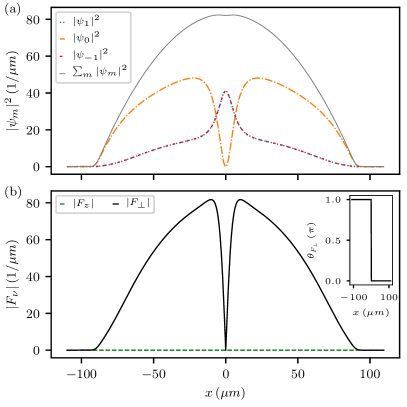
Figure 1: A typical example of an antidark-dark-antidark (ADDAD) state for $N=10000$ and $q=0.5\,n_{\mathrm{p}}\lvert c_{1}\rvert$. (a) Densities of the three components $|\psi_{m}|^{2}$, $m=\pm 1,0$, and the total density $\sum_{m}|\psi_{m}|^{2}$ (solid grey line). The total density shows a small suppression at the position of the ADDAD state. The $m_{\mathrm{F}}=0$ component carries the dark soliton (dash-dotted orange line). (b) Main frame: Amplitudes of the different components of the magnetization $\lvert F_{\nu}\rvert$, with $\nu=z,\perp$. The ADDAD state has no $F_{z}$ magnetization (dashed green line), but features a dark soliton in the transversal spin $F_{\perp}=\lvert F_{\perp}\rvert\exp\{i\,\theta_{F_{\perp}}\}$ characterized by an amplitude suppression (see solid black line in the main frame) and a corresponding phase jump (see solid black line in the inset).

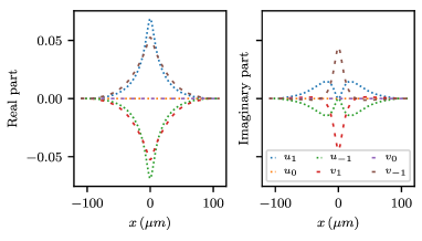
Figure 2: Real and imaginary parts of the normalized mode functions $u_{m}$, $v_{m}$ with $m=\pm 1,0$ of the unstable eigendirection of the ADDAD state for $N=10000$ and $q=0.5\,n_{\mathrm{p}}\lvert c_{1}\rvert$ as obtained from the numerical evaluation of the respective BdG equations. The corresponding mode frequency is purely imaginary leading to an exponential growth of the depicted unstable eigenmode.

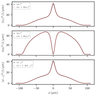
Figure 3: Comparison of the density profiles $\rvert\psi_{m}\lvert^{2}$, $m=\pm 1,0$ (solid black lines), of the ADDAD state for $N=10000$ and $q=0.5\,n_{\mathrm{p}}\lvert c_{1}\rvert$ with the profiles $\rvert\psi_{m}+\Delta\psi_{m}\lvert^{2}$ (red dotted lines) resulting from adding an exaggerated perturbation of the unstable eigenmode. The perturbation is chosen as $\Delta\psi_{m}=C(u_{m}+v_{m}^{*})$ with $C=20$ and mode functions $u_{m}$, $v_{m}$ as depicted in Fig. 2. The unstable eigenmode causes a symmetry breaking between the $m_{\mathrm{F}}=\pm 1$ components.

III Numerical Methods

Our numerical investigation of the ADDAD and DADD states involves three steps:

1. To find these solitonic structures for a given parameter set within the easy-plane phase of a spin-1 Bose gas, we employ an exact Newton-Raphson (hereafter referred to, for simplicity, as just Newton) iterative scheme to the dimensionless, time-independent versions of the equations of motion (II) and (2), see App. A. For details on the applied Newton iterative scheme, see App. B and Schmied et al. (2020). To converge to the ADDAD state within the easy-plane phase, we start the Newton iteration with the initial “guess”

   $$\begin{pmatrix}\psi_{1}\\ \psi_{0}\\ \psi_{-1}\end{pmatrix}\sim\sqrt{\frac{\mu_{\mathrm{TF}}-V(x)}{c_{0}}}\Theta\left(R_{\mathrm{TF}}^{2}-x^{2}\right)\begin{pmatrix}1\\ \tanh\left[\frac{x-x_{0}}{2\lambda}\right]\\ 1\end{pmatrix},$$ (8)

   where $x_{0}$ is the center position of the soliton and $\lambda$ quantifies the width of the hyperbolic tangent. The Heaviside theta function $\Theta$ is defined as $\Theta(z)=1$ for $z\geq 0$. We place the soliton at the trap center such that we set $x_{0}=0$. We further take the parameter $\lambda$ to be on the order of the spin healing length $\xi_{s}$ at the trap center. We choose a Thomas-Fermi (inverted parabolic) background profile Pitaevskii and Stringari (2016) as we work in a regime of comparatively large $N$ where the energy associated with the non-linear terms is considerably larger than the kinetic energy. Due to the density-density coupling $c_{0}$ being two orders of magnitude larger than the spin-spin coupling $c_{1}$, it is reasonable to take a one-dimensional Thomas-Fermi profile characterized by $c_{0}$, the trapping potential $V(x)=(1/2)M\omega_{\parallel}^{2}x^{2}$ and the corresponding Thomas-Fermi chemical potential $\mu_{\mathrm{TF}}=(1/2)\left(3\sqrt{M}c_{0}\omega_{\parallel}N/2\right)^{2/3}$. The associated Thomas-Fermi radius $R_{\mathrm{TF}}$ is defined via $V(x=R_{\mathrm{TF}})=\mu_{\mathrm{TF}}$. It is worthwhile to note that near the linear limit, i.e., for a weak nonlinearity (small $N$), the Thomas-Fermi profile has to be replaced by a Gaussian to obtain an adequate initial guess for the Newton iteration scheme. For the system studied in this work, we find that the background profile gradually approaches a Gaussian for $N\lesssim 250$; for such small values of $N$, the mean-field description is no longer expected to remain valid, yet it is of mathematical interest in its own right. We remark that the Newton iteration converges to the desired solitonic state for both, the Thomas-Fermi and the Gaussian background density profile. However, we generally observe that the more accurate the initial guess, the faster the convergence of the Newton iteration. Irrespective of the background profile, the presence of the hyperbolic tangent profile in the component bearing the dark soliton will spontaneously play the role of an attractive potential well leading to a mass of atoms in the other two components.

   To converge to the DADD state, we start the Newton iteration with the initial “guess”

   $$\begin{pmatrix}\psi_{1}\\ \psi_{0}\\ \psi_{-1}\end{pmatrix}\sim\sqrt{\frac{\mu_{\mathrm{TF}}-V(x)}{c_{0}}}\Theta\left(R_{\mathrm{TF}}^{2}-x^{2}\right)\begin{pmatrix}\tanh\left[\frac{x-x_{0}}{2\lambda}\right]\\ 1\\ \tanh\left[\frac{x-x_{0}}{2\lambda}\right]\end{pmatrix}.$$ (9)

   As indicated also above, converging to the ADDAD or DADD state does not require any knowledge about the form of the anti-dark(s) in the initial “guess” for the Newton scheme. The crucial part is the presence of a phase jump and an amplitude suppression in the desired dark component(s).

2. Upon converging to the ADDAD and DADD states by means of the Newton scheme for a particular set of parameters, we subsequently study their stability properties. These properties are extracted by numerically solving the Bogoliubov de-Gennes (BdG) equations, obtained by considering small perturbations about the solitonic states to linear order. To obtain the BdG equations, we take the Ansatz

   $$\psi_{m}(x,t)=\left[\Phi_{m}(x)+\epsilon\,\delta\psi_{m}(x,t)\right]e^{-i\mu t},$$ (10)

   with $m=\pm 1,0$ labeling the three hyperfine components and $\Phi_{m}(x)$ being the wave function of each component of the respective solitonic state obtained from the Newton scheme. Here, $\mu$ is the corresponding chemical potential, $\epsilon$ is a small parameter with $\epsilon\ll 1$ and $\delta\psi_{m}$ is the perturbation about the solitonic state. For the perturbation, we write

   $$\delta\psi_{m}(x,t)=u_{m}(x)e^{-i\omega t}+v_{m}^{*}(x)e^{i\omega^{*}t},$$ (11)

   with mode frequency $\omega$ and mode functions $u_{m},v_{m}$. For the resulting BdG equations and further details on the method see App. C and Schmied et al. (2020). Solving the BdG equations yields the eigenmodes and the respective mode frequencies of excitations about the investigated state. If all mode frequencies are real, the state is dynamically stable. Eigenmodes corresponding to mode frequencies with a non-zero imaginary part are dynamically unstable as they grow in time. Their growth rate $\gamma$ is given by the magnitude of the imaginary part of the mode frequency. Due to a finite accuracy of the solver used to evaluate the BdG equations, we consider eigenmodes to be unstable only when the imaginary part is larger than $10^{-3}$. Unstable modes can be of two different kinds. If the mode frequencies are purely imaginary, we speak of an exponential instability as the associated mode occupation grows exponentially in time. If the mode frequencies are complex, the instability is of oscillatory nature, i.e., the growth is accompanied by oscillations.

3. In the case that the BdG analysis reveals the ADDAD or DADD state to be dynamically unstable for a given parameter setting, we aim at investigating the dynamical evolution of the respective state. We then compute the time evolution of the mean-field model by solving the equations of motion (II) and (2) in dimensionless form by means of a spectral split-step algorithm. As initial configurations for the respective simulations, we take the ADDAD and DADD states as obtained from the Newton scheme and add a small perturbation to the unstable eigendirection(s) resulting from the respective BdG analysis in order to seed the instability.

IV Numerical results

In this section, we present our numerical results concerning the ADDAD and DADD states. We start by investigating the key features of the ADDAD states in Sect. IV.1 followed by the DADD states in Sect. IV.2.

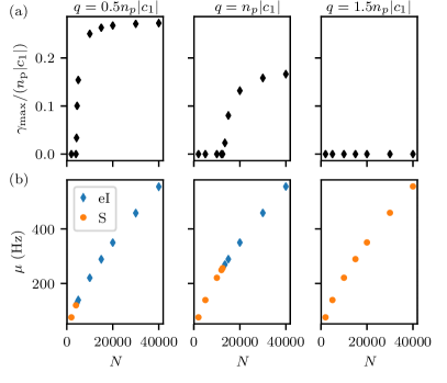
Figure 4: Stability properties of the ADDAD state for a mono-parametric continuation over the atom number $N$ for three values of the quadratic Zeeman energy $q=0.5\,n_{\mathrm{p}}\lvert c_{1}\rvert$ (left column), $q=n_{\mathrm{p}}\lvert c_{1}\rvert$ (middle column) and $q=1.5\,n_{\mathrm{p}}\lvert c_{1}\rvert$ (right column). (a) Maximal instability growth rates $\gamma_{\mathrm{max}}$ in units of $n_{\mathrm{p}}\lvert c_{1}\rvert$. The ADDAD structure becomes more stable for larger $q$. For $q=1.5\,n_{\mathrm{p}}\lvert c_{1}\rvert$, the state is dynamically stable for all $N$ considered. (b) Bifurcation diagram showing the chemical potential $\mu$ as a function of the number of atoms $N$. Stability of the ADDAD state is represented by orange circles, while exponential instability is shown by blue diamonds.

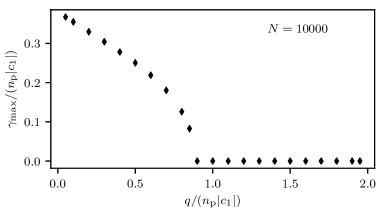
Figure 5: An addition to Fig. 4, now showing the stability quantified by the maximal instability growth rate $\gamma_{\mathrm{max}}$ as a function of $q$ for a fixed value of $N=10000$ atoms. Again, it can be seen that larger $q$’s lead to a reduced instability growth rate and eventually to a complete stabilization of the ADDAD structure for $q\gtrsim 0.9\,n_{\mathrm{p}}\lvert c_{1}\rvert$ for this value of $N$. The growth rates and the quadratic Zeeman energies are measured in units of $n_{\mathrm{p}}\lvert c_{1}\rvert$.

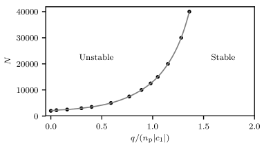
Figure 6: Stability of the ADDAD state within the ($q$,$N$)-plane. The black dots mark the boundary between the unstable and stable region of the ADDAD for selected atom numbers. The grey line is a cubic interpolation of the data points. The ADDAD becomes more dynamically stable when increasing $q$. The quadratic Zeeman energy $q$ is measured in units of $n_{\mathrm{p}}\lvert c_{1}\rvert$.

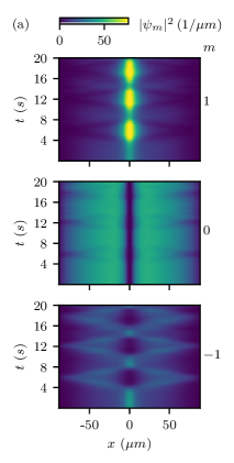
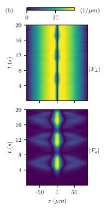
Figure 7: Time evolution of an unstable ADDAD state for $N=10000$ and $q=0.5\,n_{\mathrm{p}}\lvert c_{1}\rvert$. (a) Densities of the three components $\lvert\psi_{m}\rvert^{2}$, $m=\pm 1,0$. The symmetry breaking nature of the destabilizing dynamics can be observed between the $m_{\mathrm{F}}=\pm 1$ components. (b) Amplitudes of the different spin components $\lvert F_{\nu}\rvert$, $\nu=z,\perp$. The persistence of a dark solitonic state in the $m_{\mathrm{F}}=0$ component is confirmed through the dynamics of $F_{\perp}$ (top panel), while the asymmetry becomes visible through the nontrivial oscillations of $F_{z}$ (bottom panel).

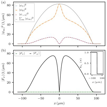
Figure 8: A typical example of a dark-antidark-dark (DADD) state for $N=10000$ and $q=0.5\,n_{\mathrm{p}}\lvert c_{1}\rvert$. (a) Densities of the three components $|\psi_{m}|^{2}$, $m=\pm 1,0$, and the total density $\sum_{m}|\psi_{m}|^{2}$ (solid grey line). The total density shows a tiny suppression at the position of the DADD state. The $m_{\mathrm{F}}=\pm 1$ components carry the dark solitons (dotted blue and dashed red lines). (b) Main frame: Amplitudes of the different components of the magnetization $\lvert F_{\nu}\rvert$, with $\nu=z,\perp$. The DADD state has no $F_{z}$ magnetization (dashed green line), but features a dark soliton in the transversal spin $F_{\perp}=\lvert F_{\perp}\rvert\exp\{i\,\theta_{F_{\perp}}\}$ characterized by an amplitude suppression (see solid black line in the main frame) and a corresponding phase jump (see solid black line in the inset).

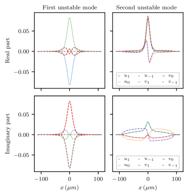
Figure 9: Real and imaginary parts of the normalized mode functions $u_{m}$, $v_{m}$ with $m=\pm 1,0$ of the two unstable eigendirections of the DADD state for $N=10000$ and $q=0.5\,n_{\mathrm{p}}\lvert c_{1}\rvert$ as obtained from the numerical evaluation of the respective BdG equations. The corresponding mode frequencies are purely imaginary leading to an exponential growth of the depicted unstable eigenmodes. The instability growth rate of the first eigenmode (left panel) is significantly larger than for the second eigenmode (right panel). Hence, the instability predominantly stems from the most unstable eigendirection.

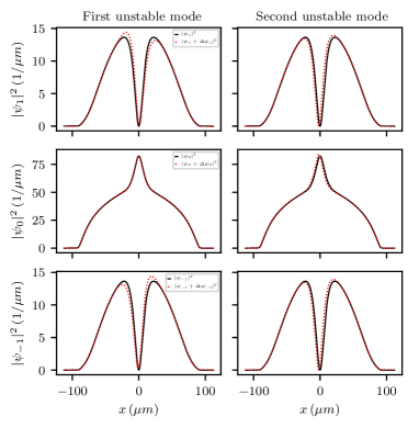
Figure 10: Comparison of the density profiles $\rvert\psi_{m}\lvert^{2}$, $m=\pm 1,0$ (solid black lines), of the DADD state for $N=10000$ and $q=0.5\,n_{\mathrm{p}}\lvert c_{1}\rvert$ with the profiles $\rvert\psi_{m}+\Delta\psi_{m}\lvert^{2}$ (red dotted lines) resulting from adding exaggerated perturbations of the first (left column) and second (right column) unstable eigenmode. The perturbations are chosen as $\Delta\psi_{m}=C(u_{m}+v_{m}^{*})$ with $C=15$ and mode functions $u_{m}$, $v_{m}$ as depicted in Fig. 9. The first (most) unstable eigenmode, that will be observed below to be dominant in the dynamics, breaks the symmetry between the $m_{\mathrm{F}}=\pm 1$ components resulting in an opposite-directed motion of these components. This eventually leads to a splitting of the DADD state. The second unstable eigenmode is a translational mode as it shifts all three components equally (in the case shown here to the left).

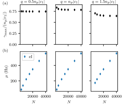
Figure 11: Stability properties of the DADD state for a mono-parametric continuation over the atom number $N$ for three values of the quadratic Zeeman energy $q=0.5\,n_{\mathrm{p}}\lvert c_{1}\rvert$ (left column), $q=n_{\mathrm{p}}\lvert c_{1}\rvert$ (middle column) and $q=1.5\,n_{\mathrm{p}}\lvert c_{1}\rvert$ (right column). (a) Maximal instability growth rates $\gamma_{\mathrm{max}}$ in units of $n_{\mathrm{p}}\lvert c_{1}\rvert$. The DADD structure is considerably less stable than the ADDAD state (cf. Fig. 4). In particular, it is generically unstable for the parameters considered with a nontrivial instability growth rate. (b) Bifurcation diagram showing the chemical potential $\mu$ as a function of the number of atoms $N$. The exponential instability of the DADD state is represented by blue diamonds. Note that for $q=1.5\,n_{\mathrm{p}}\lvert c_{1}\rvert$ a minimal atom number of $N\simeq 7000$ is needed to have a sufficient amount of atoms in the $m_{\mathrm{F}}=\pm 1$ components.

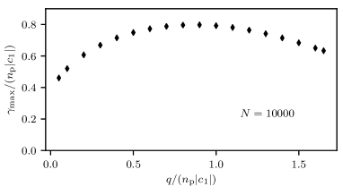
Figure 12: An addition to Fig. 11, now showing the stability quantified by the maximal instability growth rate $\gamma_{\mathrm{max}}$ as a function of $q$ for a fixed value of $N=10000$ atoms. The DADD structure is unstable within the entire parameter regime. The growth rate is largest at $q\simeq 0.9\,n_{\mathrm{p}}\lvert c_{1}\rvert$ and drops by a factor of $\simeq 2$ as $q\rightarrow 0$. For $q>1.65\,n_{\mathrm{p}}\lvert c_{1}\rvert$ the amount of atoms in the $m_{\mathrm{F}}=\pm 1$ components becomes too small to observe a true DADD structure. The growth rates and the quadratic Zeeman energies are measured in units of $n_{\mathrm{p}}\lvert c_{1}\rvert$.

IV.1 ADDAD Solitons

A typical example of the ADDAD structure obtained by means of the exact Newton scheme for a total atom number of $N=10000$ and a quadratic Zeeman energy of $q=0.5\,n_{\mathrm{p}}\lvert c_{1}\rvert$ is shown in Fig. 1. It can be seen that the dark soliton in the $m_{\mathrm{F}}=0$ component [dashed-dotted line in Fig. 1(a)] creates an effective potential attracting atoms from the two other components [dotted blue and dashed red lines in Fig. 1(a)], and forming the anti-dark spikes in these. Given the symmetry of the $m_{\mathrm{F}}=\pm 1$ states, there is no $F_{z}$ magnetization in this case [see green dashed line in Fig. 1(b)], yet the imprint of the dark soliton leads the transverse component of the magnetization $F_{\perp}$ to possess also a dark solitonic structure characterized by an amplitude suppression and an associated phase jump [black solid lines in Fig. 1(b)].

Performing the BdG analysis, we find that the potential instability of the ADDAD is characterized by one unstable eigendirection associated with the presence of one dark soliton. When an instability is present, the corresponding mode frequency is purely imaginary resulting in an exponential growth of the unstable mode. From the respective mode functions (see Fig. 2) which are only non-zero for the $m_{\mathrm{F}}=\pm 1$ components, we infer that the instability acts on the two anti-darks. The actual effect of the unstable eigendirection can be deduced by comparing the density profiles of the ADDAD state with the profiles obtained by adding an exaggerated perturbation of the unstable eigenmode to the state (see Fig. 3). We find the unstable eigendirection to cause a symmetry breaking between the $m_{\mathrm{F}}=\pm 1$ components as the perturbation increases the anti-dark’s mass in the $m_{\mathrm{F}}=1$ component while it decreases the mass in the $m_{\mathrm{F}}=-1$ component. We will discuss the resulting dynamical evolution of the unstable ADDAD state and the corresponding manifestation of this symmetry breaking effect further below.

The main results of our systematic investigation of the stability of the ADDAD state are summarized in Figs. (4)–(6). Fig. 4(a) shows the maximal instability growth rate $\gamma_{\mathrm{max}}$ as a function of the total atom number $N$ for three typical values of the quadratic Zeeman energy within the easy-plane phase. It can be observed that the larger $q$, the wider the interval of stability of the ADDAD state with respect to $N$. In fact, for $q=1.5\,n_{\mathrm{p}}\lvert c_{1}\rvert$, the state is dynamically stable for all atom numbers considered. As $q$ is lowered, the stability threshold of the state $N_{c}$ decreases. For $q=0.5\,n_{\mathrm{p}}\lvert c_{1}\rvert$, stable structures only exist for $N\lesssim 2500$. Fig. 4(b) contains the standard continuation diagram of the chemical potential $\mu$ as a function of $N$ for the different $q$’s representing stability by orange circles and exponential instability by blue diamonds. A complementary perspective, fixing the atom number to $N=10000$ and varying $q$, is presented in Fig. 5. It can be seen that up to $q\simeq 0.9\,n_{\mathrm{p}}\lvert c_{1}\rvert$, the structure is unstable for this atom number but as $q$ acquires larger values, the ADDAD state is dynamically stabilized. The possible parameter continuation over both, the atom number as well as the quadratic Zeeman energy, further allows to determine the stable and unstable regions of the ADDAD state within the respective ($q$,$N$)-plane (see Fig. 6). The extracted phase boundary between both regions clearly shows that the ADDAD becomes more dynamically stable for larger quadratic Zeeman energies and for smaller atom numbers. Notice that the enhanced stability of the state for larger $q$ can be qualitatively understood by the fact that as $q$ increases, the $m_{\mathrm{F}}=\pm 1$ anti-dark components are suppressed, ultimately leading to a single dark soliton which is a stable state in the polar phase of the spinor system.

We now turn to the examination of the dynamical instability of the ADDAD state. We illustrate a typical time evolution for $N=10000$ and $q=0.5\,n_{\mathrm{p}}\lvert c_{1}\rvert$ in Fig. 7. Here, we perturb the unstable eigendirection according to the BdG formulation in Eqs. (10) and (11) such that the amplitude of the perturbation is $0.1\%$ of the amplitude of the $m_{\mathrm{F}}=\pm 1$ components of the ADDAD state obtained from the Newton scheme. It can be seen that the ADDAD suffers a symmetry breaking leading to an asymmetric partition of the anti-dark components as expected from the perturbed density profiles depicted in Fig. 3. This means, that one of the two $m_{\mathrm{F}}=\pm 1$ states acquires more atoms than the other and subsequently, given the Hamiltonian nature of the model, an oscillatory dynamics ensues between the unstable symmetric state and the presumably more dynamically robust asymmetric state [see Fig. 7(a)]. During this observed oscillation, the dark solitonic structure persists in the transversal spin $F_{\perp}$ [see top panel of Fig. 7(b)], while at the same time the asymmetry bestows a nontrivial oscillatory dynamics in $F_{z}$ [see bottom panel of Fig. 7(b)]. We expect the symmetry breaking to occur when the amplitude of the unstable mode becomes similar to the amplitude of the $m_{\mathrm{F}}=\pm 1$ components of the initial ADDAD state. Hence, an estimate for the corresponding break-up time $t_{\mathrm{b}}\simeq-(\log A)/\gamma_{\mathrm{max}}=4\,s$ can directly be inferred from the respective instability growth rate $\gamma_{\mathrm{max}}=0.25\,n_{\mathrm{p}}\lvert c_{1}\rvert$ and the relative amplitude of the perturbation $A=0.001$. Note that the estimate for $t_{\mathrm{b}}$ agrees remarkably well with the break-up time observed in the numerical simulation [cf. Fig. 7(a)]. Small deviations may arise from additional non-linear effects.

IV.2 DADD Solitons

Similar features as discussed for the ADDAD structure can be obtained for the DADD soliton. A typical example of the DADD structure for a total atom number of $N=10000$ and a quadratic Zeeman energy of $q=0.5\,n_{\mathrm{p}}\lvert c_{1}\rvert$ is presented in Fig. 8. It can be seen that the two dark solitons in the $m_{\mathrm{F}}=\pm 1$ components [dotted blue and dashed red lines in Fig. 8(a)] create an effective potential attracting atoms from the $m_{\mathrm{F}}=0$ component [dash-dotted orange line in Fig. 8(a)], and forming the anti-dark spike in the latter. Given the symmetry between the $m_{\mathrm{F}}=\pm 1$ states, there is also no $F_{z}$ magnetization in this case [green dashed line in Fig. 8(b)], yet the imprint of the dark soliton leads the transverse component of the magnetization $F_{\perp}$ to possess also a dark solitonic structure characterized by an amplitude suppression and an associated phase jump [black solid lines in Fig. 8(b)].

Performing the BdG analysis, we find that an instability of the DADD is characterized by two unstable eigendirections associated with the fact that the state features two dark solitons. The corresponding eigenfrequencies (generically) are purely imaginary resulting in an exponential growth of the unstable modes. However, one of the eigendirections exhibits a significantly larger growth rate $\gamma$ than the other, hence we expect this unstable eigenmode to dominate the instability. From the respective mode functions of the most unstable eigendirection (see left column in Fig. 9) which are only non-zero for the $m_{\mathrm{F}}=\pm 1$ components, we infer that the instability acts on the two dark solitons. As we did previously for the ADDAD state, we compare the density profiles of the DADD state with the profiles obtained by adding an exaggerated perturbation of each of the unstable eigenmodes to the state to deduce the actual effect of the unstable eigendirections (see Fig. 10). The symmetry breaking nature of the most unstable eigendirection causes the $m_{\mathrm{F}}=\pm 1$ components to move in opposite directions (see left column in Fig. 10). This induces a splitting of the DADD state in the dynamical evolution which will be discussed further below. The second unstable eigenmode is a translational mode as it shifts all three $m_{\mathrm{F}}$-components equally in the same direction (see right column in Fig. 10).

The main conclusions of our systematic numerical computations as regards the dynamical stability of the DADD structures are captured in Figs. 11 and 12 and can be summarized as follows. Generally speaking, DADD structures are considerably less stable than the ADDADs. We suspect that this has to do with the more highly excited nature of the DADD state involving more dark solitons than the ADDAD state. In fact, this has been illustrated in lower component analyses where it was found that the higher the number of dark solitons, the more potentially unstable modes exist in the system Kevrekidis et al. (2015). What can be clearly discerned in the different panels of Fig. 11 is that no stabilization of the structures is found in our mono-parametric continuation over the number of atoms $N$, for different values of the quadratic Zeeman energy $q$. While for larger values of $N$, the instability appears to slightly weaken, which can be inferred from the lower maximal instability growth rate $\gamma_{\mathrm{max}}$, it does not seem to asymptote towards $\gamma_{\mathrm{max}}\rightarrow 0$ and remains always substantially larger than in the previously discussed case of the ADDADs (cf. Fig. 4). A complementary perspective, fixing the atom number to $N=10000$ and varying $q$ systematically, is presented in Fig. 12. It can be clearly seen that the DADD state is generically unstable within the entire easy-plane phase. In particular, it is found to be most unstable for $q\simeq 0.9n_{\mathrm{p}}\lvert c_{1}\rvert$. Approaching the phase boundaries at $q=2n_{\mathrm{p}}\lvert c_{1}\rvert$ and $q=0$, the instability growth rate decreases, leading to the observed non-monotonic dependence on $q$. In the former case, the configuration passes over to a single-component (stable) ground state (of the polar phase), while in the latter one it tends to a two-component dark soliton which is more robust than its spinor counterpart.

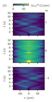
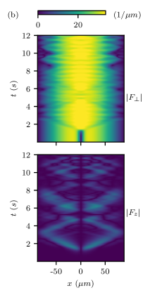
Figure 13: Time evolution of an unstable DADD state for $N=10000$ and $q=0.5\,n_{\mathrm{p}}\lvert c_{1}\rvert$. (a) Densities of the three components $\lvert\psi_{m}\rvert^{2}$, $m=\pm 1,0$. The three panels reveal the definitive splitting of the DADD into a left- and a right-moving structure, with the anti-dark being shifted to the $m_{\mathrm{F}}=1$ and $m_{\mathrm{F}}=-1$ component, respectively, while the $m_{\mathrm{F}}=0$ component breaks into a pair of gray solitary waves. Note that the emerging moving structures are not dynamically robust resulting in their eventual dispersion over long timescales. (b) Amplitudes of the different spin components $\lvert F_{\nu}\rvert$, $\nu=z,\perp$. In correspondence with (a), we observe a splitting of the $F_{\perp}$ profile (top panel) concurrently with the generation of two oppositely-moving waves in the $F_{z}$ magnetization (bottom panel). After one oscillation in the trap the waves seem to disperse.

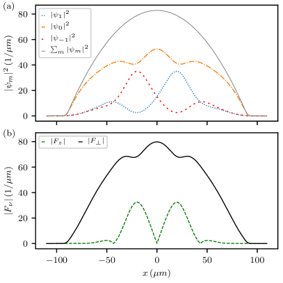
Figure 14: Unstable DADD state shortly after the splitting (evolution time $t\simeq 1.7\,s$) for $N=10000$ and $q=0.5\,n_{\mathrm{p}}\lvert c_{1}\rvert$. (a) Densities of the three components $|\psi_{m}|^{2}$, $m=\pm 1,0$, and the total density $\sum_{m}|\psi_{m}|^{2}$ (solid grey line). The left- and right-moving gray solitons in the $m_{\mathrm{F}}=\mp 1$ components are accompanied by respective anti-darks in the $m_{\mathrm{F}}=\pm 1$ components and shallow gray solitons the $m_{\mathrm{F}}=0$ component. (b) Amplitudes of the different components of the magnetization $\lvert F_{\nu}\rvert$, with $\nu=z,\perp$. Due to the asymmetry between the $m_{\mathrm{F}}=\pm 1$ components in the left- and right-moving structures, we observe a non-zero local $F_{z}$ magnetization (dashed green line).

The overwhelmingly more unstable nature of the DADD structures naturally raises the question of the dynamical implications of this instability. This is clarified in the dynamical evolution of the DADD state for a prototypical case with $N=10000$ and $q=0.5\,n_{\mathrm{p}}\lvert c_{1}\rvert$ depicted in Fig. 13. Here, we perturb the two unstable eigendirections according to the BdG formulation in Eqs. (10) and (11) such that the amplitude of the perturbation is $0.1\%$ of the amplitude of the $m_{\mathrm{F}}=\pm 1$ components of the DADD state obtained from the Newton scheme. In as far as we have been able to observe in our numerical simulations, the time evolution shown is representative for the relevant dynamics. From the perturbed density profiles in Fig. 10 we already observed that the instability eigenvector corresponding to the most unstable eigendirection breaks the symmetry between the two dark solitons in the $m_{\mathrm{F}}=\pm 1$ components inducing an opposite-directed motion. This leads to a splitting of the DADD [see Fig. 13(a) and Fig. 14 for a slice of the density and spin profiles at $t\simeq 1.7\,s$, i.e., shortly after the splitting] whereby for example the dark soliton in the $m_{\mathrm{F}}=-1$ component captures part of the mass from the anti-dark in the $m_{\mathrm{F}}=0$ component such that it becomes gray and moves to the left. Within this process, another fraction of the $m_{\mathrm{F}}=0$-state’s anti-dark mass is captured by the $m_{\mathrm{F}}=1$ component where an anti-dark soliton emerges. As a consequence, the corresponding $m_{\mathrm{F}}=0$ component is found to feature an amplitude suppression in the form of a gray solitary wave after the splitting. The entire structure appears to be again of DADD type with the anti-dark being shifted to the $m_{\mathrm{F}}=1$ component while a gray solitary wave is present in the $m_{\mathrm{F}}=0$ component. Analogously, the right-moving structure is also of DADD type with the anti-dark being shifted to the $m_{\mathrm{F}}=-1$ component and another gray soliton arising in the $m_{\mathrm{F}}=0$ component. Again, we expect the splitting to occur when the amplitude of the most unstable mode becomes similar to the amplitude of the $m_{\mathrm{F}}=\pm 1$ components of the initial DADD state. Accordingly, an estimate for the break-up time $t_{\mathrm{b}}\simeq-(\log A)/\gamma_{\mathrm{max}}=1.33\,s$ can directly be inferred from the respective instability growth rate $\gamma_{\mathrm{max}}=0.75\,n_{\mathrm{p}}\lvert c1\rvert$ and the relative amplitude of the perturbation $A=0.001$. Note that once again the estimate for $t_{\mathrm{b}}$ agrees remarkably well with the break-up time observed in the numerical simulation [cf. Fig. 13(a)]. We remark that the structures emerging after the splitting of the DADD are not dynamically robust and quickly generate additional excitations in the system leading to an eventual dispersion over long timescales. We have observed this type of splitting and the creation of moving solitary waves in the entire range of $q$ values depicted in Fig. 12. We find the emerging states to become more robust as $q\rightarrow 0$. We attribute this property to the increasing fraction of atoms in the $m_{\mathrm{F}}=\pm 1$ components with respect to the $m_{\mathrm{F}}=0$ component in the initial DADD structure.

V Conclusion and outlook

In this work, we numerically showed the existence of DADD and ADDAD solitonic states within the easy-plane phase of a ferromagnetic trapped one-dimensional spin-1 Bose gas. Furthermore, we investigated their stability properties by solving the respective BdG equations. In particular, we elaborated on the stability of the states for a continuation over the total atom number and the quadratic Zeeman energy. The identified potential dynamical instabilities of the states were complemented with direct numerical simulations elucidating the corresponding dynamics.

Our key observation is that the ADDAD structure is more robust than the DADD state which is found to be unstable in all parameter regimes considered. We suspect that these findings stem from the more highly excited nature of the DADD state bearing two dark solitons rather than one. Studying the time evolution of an unstable DADD state revealed that it breaks up into a left- and right-moving pair of dark-antidark states accompanied by a redistribution of the solitary waves between the components and the eventual dispersion of the resulting structures. However, the evolution of an unstable ADDAD state generated an asymmetric distribution of the anti-darks involving an oscillatory dynamics of the $F_{z}$ magnetization. Nevertheless, the ADDAD structure could be stabilized in suitable regimes in parameter space and hence be accessible to the recent experimental observations in spinor systems Bersano et al. (2018); Lannig et al. (2020).

An interesting future direction would be to generate multiple such solitary waves and examine in their interactions as it was done recently for BDB solitons in Lannig et al. (2020). Going one step further, it may be possible to engineer soliton lattices or random soliton gases Schwache and Mitschke (1997); Schmidt et al. (2012); Wang and Kevrekidis (2015); Redor et al. (2019) of these three-component structures and study their collisional properties in the spin degree of freedom. Lastly, it appears especially relevant to consider generalizations of such states to higher-dimensional configurations, involving topologically charged coherent structures. In addition to a scenario of two vortices trapping an anti-dark wave and a single vortex trapping two anti-darks, further possibilities emerge given that the multiple vortices can bear the same or opposite topological charge. Additionally, both two-dimensional and three-dimensional extensions of linear, planar, or spherical Kevrekidis et al. (2015); Frantzeskakis (2010) dark solitons trapping corresponding anti-dark states may be accessible and quite interesting for future work, especially given their potential transverse instabilities and associated dynamics.

Acknowledgments. The authors thank T. Gasenzer for his valuable comments that helped us to significantly improve our manuscript and M. K. Oberthaler for discussions and collaboration on the topics described here. P. G. K. additionally acknowledges discussions with S. I. Mistakidis and G. C. Katsimiga on spinor condensates. This work was supported by the Heidelberg Graduate School of Fundamental Physics (HGSFP), the Heidelberg Center for Quantum Dynamics (CQD), the European Commission, within the Horizon-2020 programme, through the ERC Advanced Grant EntangleGen (Project-ID 694561) as well as the Deutsche Forschungsgemeinschaft (DFG, German Research Foundation) – Project-ID 273811115 – SFB 1225. This material is based upon work supported by the US National Science Foundation under Grants No. PHY-1602994 and DMS-1809074 and by the Alexander von Humboldt Foundation. P. G. K. further acknowledges support from the Leverhulme Trust via a Visiting Fellowship and thanks the Mathematical Institute of the University of Oxford for its hospitality during part of this work.

APPENDIX

In the appendix, we briefly elaborate on the numerical methods used to show the existence and to study the stability properties of the ADDAD and DADD states. The following discussion is partly taken and adapted from Schmied et al. (2020), where the interested reader can also find additional details on the numerical schemes.

Appendix A Time-independent equations of motion

In this work, we are interested in ADDAD and DADD solitons that are stationary states of the equations of motion (II) and (2). Hence, we aim to identify solutions to the time-independent version of these equations. By choosing the Ansatz $\psi_{m}(x,t)=\psi_{m}(x)e^{-i\mu_{m}t}$ with $m=\pm 1,0$ and $\mu_{m}$ being the chemical potential of each spinor component, a stationary state resulting from Eqs. (II) and (2) has to fulfill the phase matching condition $2\mu_{0}-\mu_{1}-\mu_{-1}=0$. As a population imbalance between the $m_{\mathrm{F}}=\pm 1$ components is not favored, independent of the choice of the couplings in the equations of motion, we assume that $\mu_{1}=\mu_{-1}$ here, which implies that $\mu_{0}=\mu_{1}=\mu_{-1}\equiv\mu$. The time-independent equations of motion (in dimensionless form according to the definitions in the main text) then read:

$$\mathcal{F}_{\pm 1}(\psi_{1},\psi_{0},\psi_{-1},\psi_{1}^{*},\psi_{0}^{*},\psi_{-1}^{*})\equiv -\mu\psi_{\pm 1}+H_{0}\psi_{\pm 1}+q\psi_{\pm 1}$$

$$+c_{1}\left(\lvert\psi_{\pm 1}\lvert^{2}+\lvert\psi_{0}\lvert^{2}-\lvert\psi_{\mp 1}\lvert^{2}\right)\psi_{\pm 1}$$

$$+c_{1}\psi_{0}^{2}\psi_{\mp 1}^{*}$$

$$= \,0,$$ (1)

$$\mathcal{F}_{0}(\psi_{1},\psi_{0},\psi_{-1},\psi_{1}^{*},\psi_{0}^{*},\psi_{-1}^{*})\equiv -\mu\psi_{0}+H_{0}\psi_{0}$$

$$+c_{1}\left(\lvert\psi_{1}\lvert^{2}+\lvert\psi_{-1}\lvert^{2}\right)\psi_{0}$$

$$+2c_{1}\psi_{-1}\psi_{0}^{*}\psi_{1}$$

$$= \,0.$$ (2)

Here, we introduced functions $\mathcal{F}_{0,\pm 1}$ as abbreviations for the time-independent equations of motion which will be of practical use for discussing the Newton scheme (see App. B) as well as the Bogoliubov-de Gennes equations (see App. C).

Appendix B Iterative Newton scheme

Various first- and second-order methods can be applied to find solutions to Eqs. (A) and (A). Here, we make use of a Newton iteration scheme. It is a second-order method which involves the explicit calculation of the Jacobian. The Newton scheme is not restricted to finding ground states (i.e. the global energy minimum) of a physical system such that in case of an adequate initial “guess” for the wavefunctions, it offers the possibility to converge to the desired ADDAD and DADD states.

The Newton scheme for the spin-1 system can be cast into the form of a six-dimensional matrix equation:

$$J\Delta\psi=\mathcal{F},$$ (3)

where $\Delta\psi$ gives the correction to the wave function of the previous iteration of the Newton scheme with $\psi=(\psi_{1},\psi_{0},\psi_{-1},\psi_{1}^{*},\psi_{0}^{*},\psi_{-1}^{*})^{T}$ being a vector of all spinor fields. The vector $\mathcal{F}=(\mathcal{F}_{1},\mathcal{F}_{0},\mathcal{F}_{-1},\mathcal{F}_{1}^{*},\mathcal{F}_{0}^{*},\mathcal{F}_{-1}^{*})^{T}$ contains the time-independent equations of motion [see Eqs. (A) and (A)] as well as their complex conjugated versions. The Jacobian $J$ is given by the matrix

$$J_{ij}=\frac{\partial\mathcal{F}_{i}}{\partial\psi_{j}},$$ (4)

where $i,j\,\epsilon\,\{0,\dots,5\}$ and the partial derivative is evaluated at the wave function $\psi$ of the current iteration step.

To converge to a state with fixed atom number $N$, we further introduce a Lagrange multiplier $\lambda$ for the chemical potential $\mu$. This adds the following constraint to our Newton scheme

$$\mathcal{F}_{\lambda}\equiv\int\left(\lvert\psi_{1}\rvert^{2}+\lvert\psi_{0}\rvert^{2}+\lvert\psi_{-1}\rvert^{2}\right)\mathrm{d}x-N=0.$$ (5)

Consequently, the resulting modified scheme can be written as

$$\tilde{J}\Delta\tilde{\psi}=\tilde{\mathcal{F}},$$ (6)

with $\tilde{\psi}=(\psi_{1},\psi_{0},\psi_{-1},\psi_{1}^{*},\psi_{0}^{*},\psi_{-1}^{*},\lambda)^{T}$ and $\tilde{\mathcal{F}}=(\mathcal{F}_{1},\mathcal{F}_{0},\mathcal{F}_{-1},\mathcal{F}_{1}^{*},\mathcal{F}_{0}^{*},\mathcal{F}_{-1}^{*},\mathcal{F}_{\lambda})^{T}$. In each iteration step we calculate $\tilde{\mathcal{F}}$ and evaluate the corresponding Jacobian $\tilde{J}$ of the system. The second derivative occurring in the equations of motion is obtained by means of a second-order center difference scheme. By solving the eigenvalue equation (6), we obtain the correction to the wave function $\Delta\tilde{\psi}$. The Newton scheme terminates if the norm of the correction is smaller than the preset tolerance of $10^{-10}$.

Appendix C Bogoliubov de-Gennes equations

The stability properties of the ADDAD and DADD state are deduced from numerically solving the corresponding Bogoliubov de-Gennes (BdG) equations.

To derive the BdG equations, we consider a small perturbation about the stationary state of interest. Therefore, we take the Ansatz

$$\psi_{m}(x,t)=\left[\Phi_{m}(x)+\epsilon\,\delta\psi_{m}(x,t)\right]e^{-i\mu t},$$ (7)

with $m=\pm 1,0$ labeling the three hyperfine components and $\Phi_{m}(x)$ being the wave function of each component at the stationary state; $\mu$ is the corresponding chemical potential; $\epsilon$ is a small parameter with $\epsilon\ll 1$ and $\delta\psi_{m}$ is the perturbation about the stationary state.

Plugging the Ansatz (7) into the equations of motion (II) and (2) (in dimensionless form according to the definitions in the main text) and subsequently linearizing the resulting equations (i.e. taking contributions to order $\epsilon$) yields

$$i\partial_{t}\delta\psi_{m}= \,\,\left(\frac{\partial\mathcal{F}_{m}}{\partial\Phi_{1}}\right)_{|\Phi}\delta\psi_{1}+\left(\frac{\partial\mathcal{F}_{m}}{\partial\Phi_{0}}\right)_{|\Phi}\delta\psi_{0}+\left(\frac{\partial\mathcal{F}_{m}}{\partial\Phi_{-1}}\right)_{|\Phi}\delta\psi_{-1}$$

$$+\left(\frac{\partial\mathcal{F}_{m}}{\partial\Phi_{1}^{*}}\right)_{|\Phi}\delta\psi_{1}^{*}+\left(\frac{\partial\mathcal{F}_{m}}{\partial\Phi_{0}^{*}}\right)_{|\Phi}\delta\psi_{0}^{*}+\left(\frac{\partial\mathcal{F}_{m}}{\partial\Phi_{-1}^{*}}\right)_{|\Phi}\delta\psi_{-1}^{*}.$$ (8)

Here, the $\mathcal{F}_{m}$ are the functions introduced in Eqs. (A) and (A). The partial derivatives of $\mathcal{F}_{m}$ are taken with respect to the stationary fields and are then evaluated at $\Phi$, with $\Phi=(\Phi_{1},\Phi_{0},\Phi_{-1},\Phi_{1}^{*},\Phi_{0}^{*},\Phi_{-1}^{*})$ being a vector that contains the wave functions at the stationary state.

To solve the BdG equations, we make use of the Ansatz

$$\delta\psi_{m}(x,t)=\left(u_{m}(x)e^{-i\omega t}+v_{m}^{*}(x)e^{i\omega^{*}t}\right),$$ (9)

with mode frequency $\omega$ and mode functions $u_{m},v_{m}$. Inserting the Ansatz into Eq. (C) and matching the phase factors to obtain a time-independent description, we can write the BdG equations as an eigenvalue problem of the form

$$\bar{J}\mathcal{M}=-\omega\mathcal{M}.$$ (10)

Here, $\mathcal{M}=(u_{1},u_{0},u_{-1},v_{1},v_{0},v_{-1})^{T}$ is a vector that contains all eigenmodes of the system. The matrix $\bar{J}$ turns out to be the Jacobian introduced in Eq. (4) whose lower half of entries is multiplied by a factor of $-1$. Formally, we can write it as

$$\bar{J}_{ij}=\left[1-2\Theta(i-3)\right]\left(J_{ij}\right)_{|\Phi},$$ (11)

where $i,j\,\epsilon\,\{0,\dots,5\}$ and the Heaviside theta function $\Theta$ is defined as $\Theta(z)=1$ for $z\geq 0$.

The mode frequencies $\omega$ correspond to the eigenvalues of $\bar{J}$ and the mode functions $u_{m},v_{m}$ are given by the eigenvectors. We numerically solve the eigenvalue problem in Eq. (10) using the standard _-geev LAPACK routines in python.

References

- Pethick and Smith (2006) C. J. Pethick and H. Smith, Bose-Einstein condensation in dilute gases (CUP, Cambridge, UK, 2006).
- Pitaevskii and Stringari (2016) L. P. Pitaevskii and S. Stringari, Bose-Einstein Condensation and Superfluidity (OUP, Oxford, UK, 2016).
- Kevrekidis et al. (2015) P. G. Kevrekidis, D. J. Frantzeskakis, and R. Carretero-González, The Defocusing Nonlinear Schrödinger Equation (SIAM, Philadelphia, 2015).
- Kivshar and Agrawal (2003) Y. S. Kivshar and G. P. Agrawal, Optical solitons: from fibers to photonic crystals (Academic Press, San Diego, 2003).
- Ablowitz (2011) M. J. Ablowitz, Nonlinear Dispersive Waves (CUP, Cambridge, UK, 2011).
- Frantzeskakis (2010) D. Frantzeskakis, J. Phys. A 43, 213001 (2010).
- Fetter and Svidzinsky (2001) A. L. Fetter and A. A. Svidzinsky, J. Phys.: Cond. Mat. 13, R135 (2001).
- Fetter (2009) A. L. Fetter, Rev. Mod. Phys. 81, 647 (2009).
- Komineas (2007) S. Komineas, Eur. Phys. J. Spec. Top. 147, 133 (2007).
- Kartashov et al. (2014) Y. V. Kartashov, B. A. Malomed, Y. Shnir, and L. Torner, Phys. Rev. Lett. 113, 264101 (2014).
- Proment et al. (2012) D. Proment, M. Onorato, and C. F. Barenghi, Phys. Rev. E 85, 036306 (2012).
- Ticknor et al. (2019) C. Ticknor, V. P. Ruban, and P. G. Kevrekidis, Phys. Rev. A 99, 063604 (2019).
- Shaukat et al. (2017) M. I. Shaukat, E. V. Castro, and H. Terças, Phys. Rev. A 95, 053618 (2017).
- Kevrekidis and Frantzeskakis (2016) P. G. Kevrekidis and D. J. Frantzeskakis, Rev. Phys. 1, 140 (2016).
- Stenger et al. (1998) J. Stenger, S. Inouye, D. Stamper-Kurn, H. Miesner, A. Chikkatur, and W. Ketterle, Nature 396, 345 (1998).
- Kawaguchi and Ueda (2012) Y. Kawaguchi and M. Ueda, Phys. Rep. 520, 253 (2012).
- Stamper-Kurn and Ueda (2013) D. M. Stamper-Kurn and M. Ueda, Rev. Mod. Phys. 85, 1191 (2013).
- Prüfer et al. (2018) M. Prüfer, P. Kunkel, H. Strobel, S. Lannig, D. Linnemann, C.-M. Schmied, J. Berges, T. Gasenzer, and M. K. Oberthaler, Nature 563, 217 (2018).
- Busch and Anglin (2001) T. Busch and J. R. Anglin, Phys. Rev. Lett. 87, 010401 (2001).
- Becker et al. (2008) C. Becker, S. Stellmer, P. Soltan-Panahi, S. Dörscher, M. Baumert, E. M. Richter, J. Kronjäger, K. Bongs, and K. Sengstock, Nat. Phys. 4, 496 (2008).
- Bersano et al. (2018) T. M. Bersano, V. Gokhroo, M. A. Khamehchi, J. D’Ambroise, D. J. Frantzeskakis, P. Engels, and P. G. Kevrekidis, Phys. Rev. Lett. 120, 063202 (2018).
- Lannig et al. (2020) S. Lannig, C.-M. Schmied, M. Prüfer, P. Kunkel, R. Strohmaier, H. Strobel, T. Gasenzer, P. G. Kevrekidis, and M. K. Oberthaler, Phys. Rev. Lett. 125, 170401 (2020).
- Liu et al. (2020) I.-K. Liu, S.-C. Gou, and H. Takeuchi, Phys. Rev. Research 2, 033506 (2020).
- Katsimiga et al. (2020a) G. C. Katsimiga, S. I. Mistakidis, P. Schmelcher, and P. G. Kevrekidis, (2020a), arXiv:2008.00475 [nlin.PS] .
- Kevrekidis et al. (2004) P. G. Kevrekidis, H. E. Nistazakis, D. J. Frantzeskakis, B. A. Malomed, and R. Carretero-González, Eur. Phys. J. D28, 181 (2004).
- Danaila et al. (2016) I. Danaila, M. A. Khamehchi, V. Gokhroo, P. Engels, and P. G. Kevrekidis, Phys. Rev. A 94, 053617 (2016).
- Katsimiga et al. (2020b) G. C. Katsimiga, S. I. Mistakidis, T. M. Bersano, M. K. H. Ome, S. M. Mossman, K. Mukherjee, P. Schmelcher, P. Engels, and P. G. Kevrekidis, Phys. Rev. A 102, 023301 (2020b).
- Qu et al. (2016) C. Qu, L. P. Pitaevskii, and S. Stringari, Phys. Rev. Lett. 116, 160402 (2016).
- Chai et al. (2020) X. Chai, D. Lao, K. Fujimoto, R. Hamazaki, M. Ueda, and C. Raman, Phys. Rev. Lett. 125, 030402 (2020).
- Farolfi et al. (2020) A. Farolfi, D. Trypogeorgos, C. Mordini, G. Lamporesi, and G. Ferrari, Phys. Rev. Lett. 125, 030401 (2020).
- Schmied et al. (2020) C.-M. Schmied, T. Gasenzer, M. K. Oberthaler, and P. G. Kevrekidis, CNSNS 83, 105050 (2020).
- Dabrowska-Wüster et al. (2007) B. J. Dabrowska-Wüster, E. A. Ostrovskaya, T. J. Alexander, and Y. S. Kivshar, Phys. Rev. A 75, 023617 (2007).
- Schwache and Mitschke (1997) A. Schwache and F. Mitschke, Phys. Rev. E 55, 7720 (1997).
- Schmidt et al. (2012) M. Schmidt, S. Erne, B. Nowak, D. Sexty, and T. Gasenzer, NJP 14, 075005 (2012).
- Wang and Kevrekidis (2015) W. Wang and P. G. Kevrekidis, Phys. Rev. E 91, 032905 (2015).
- Redor et al. (2019) I. Redor, E. Barthélemy, H. Michallet, M. Onorato, and N. Mordant, Phys. Rev. Lett. 122, 214502 (2019).