Convergence of adaptive stochastic collocation with finite elements

Abstract.

We consider an elliptic partial differential equation with a random diffusion parameter discretized by a stochastic collocation method in the parameter domain and a finite element method in the spatial domain. We prove convergence of an adaptive algorithm which adaptively enriches the parameter space as well as refines the finite element meshes.

1. Introduction

We consider an adaptive stochastic collocation algorithm for a random diffusion problem proposed in [18] and extend it to include spatial mesh refinement for a finite element method. We prove convergence of the adaptive algorithm to the exact solution and even derive some convergence rates.

Problems of this kind have been considered in many prior works. See, e.g., [1, 7] for stochastic collocation methods, [13, 10] for quasi-Monte Carlo sampling approaches, [12, 14] for multi-level methods, and [11] for a multi-index method. Those non-intrusive methods have the big advantage that they do not require new solver algorithms, but reuse deterministic solvers only. Roughly speaking, the exact solution depends on a parametric variable (the random input) and a spatial variable. While the spatial dependence is resolved by standard finite element approximation, the parametric dependence is discretized by collocation. For each collocation point, we need to solve a deterministic problem and can reuse well tested finite element code for deterministic problems.

Adaptivity comes into mind for two reasons: First, the spatial adaptivity is necessary to resolve singularities originating from geometric features (e.g., concave corners) and from irregular coefficients induced by the random input. Uniform meshes suffer from drastic reduction of convergence rate in the presence of such singularities, see, e.g., [5] for an exhaustive overview on $h$-adaptive methods. Second, the parametric adaptivity is necessary to resolve anisotropy in the random coefficient. The random input can often be parametrized on high-dimensional parameter domains and, usually, not all directions of that domain are equally important. Therefore, a straightforward tensor approximation approach would suffer dramatically from the curse of dimensionality. Here, an adaptive approach can outperform uniform methods significantly, see [8, 9] for an overview.

For intrusive stochastic Galerkin methods, adaptive algorithms have been investigated in [4, 16] and for non-intrusive stochastic collocation methods, an adaptive algorithm was proposed in [18]. The work uses a sparse grid interpolation operator to discretize the parametric domain and proposes an error estimator which consists of an parametric estimator as well as a finite element estimator. We extend the algorithm of [18] and include spatial adaptivity by use of a standard $h$-adaptive algorithm inspired by [4]. Basically, we use Dörfler marking to identify a number of collocation points which require adaptive refinement of the underlying finite element mesh and then use well understood spatial adaptivity to improve the finite element error. The main difficulty is the interplay of parametric refinement and finite element refinement to ensure overall convergence.

The remainder of this work is organized as follows: We present the model problem in Section 1.1 and describe the adaptive algorithm in Section 1.3. In Section 2, we prove convergence of the adaptive algorithm for the pure parameter enrichment problem (i.e., the problem considered in [18]), and Section 3 proves the convergence of the full adaptive algorithm including spatial adaptivity. A final Section 4 presents a numerical experiment.

1.1. Problem statement

Consider a domain $D\subset\mathbb{R}^{d}$ with $d\geq 2$ and a probability space $\left(\Omega,\mathcal{F},\mathcal{P}\right)$. Let $Y_{n}:\Omega\rightarrow\mathbb{R}$ be a random variable with range $\Gamma_{n}\coloneqq Y_{n}(\Omega)$ (a bounded subset of $\mathbb{R}$) and density $\rho_{n}:\Gamma_{n}\rightarrow\mathbb{R}_{\geq 0}$ for all $n\in 1,\ldots,N$. Suppose that the $\left(Y_{n}\right)_{n=1}^{N}$ are independent. Let $\Gamma\coloneqq\bigotimes_{n=1}^{N}\Gamma_{n}\subset\mathbb{R}^{N}$ and $\rho\coloneqq\bigotimes_{n=1}^{N}\rho_{n}$. The triple ($\Gamma,\mathcal{B}(\Gamma),\rho(\bm{y})\textrm{d}\bm{y}$) ($\mathcal{B}(\Gamma)$ the Borel $\sigma$-algebra on $\Gamma$) is a probability space. Consider $f\in L^{2}(D)$ and $a:\Gamma\times D\rightarrow\mathbb{R}$ with the following properties: Uniform boundedness

$$\exists a_{min},a_{max}\in\mathbb{R}_{>0}:a_{min}\leq a(\bm{y},x)\leq a_{max}\qquad\rho\textrm{-a.e. }\bm{y}\in\Gamma,\forall x\in D.$$

and affine dependence on $\bm{y}\in\Gamma$:

$$\forall n\in 0,\ldots,N\ \exists\ a_{n}:D\rightarrow\mathbb{R}:a(\bm{y},x)=a_{0}(x)+\sum_{n=1}^{N}a_{n}(x)y_{n}.$$

The problem reads: Find $u:\Gamma\rightarrow V$ such that

(1) $$\int_{D}a(x,\bm{y})\nabla u(x,\bm{y})\cdot\nabla v(x)\textrm{d}x=\int_{D}f(x)v(x)\textrm{d}x\qquad\forall v\in V,\ \rho\textrm{-a.e.}\ \bm{y}\in\Gamma.$$

$V$ denotes the Sobolev space $H^{1}_{0}(D)$ with the norm $\norm{v}_{V}\coloneqq\norm{\nabla v}_{L^{2}(D)}$.

Due to uniform ellipticity of the problem the exact solution is unique and (see also, e.g., [1]) there exists $\bm{\tau}\subset\mathbb{R}_{>0}^{N}$ such that $u:\Gamma\rightarrow V$ can be extended to a bounded holomorphic function on the set

(2) $$\Sigma(\Gamma,\bm{\tau})\coloneqq\left\{\bm{z}\in\mathbb{C}^{N}:dist(z_{n},\Gamma_{n})\leq\tau_{n}\ \forall n=1,\ldots,N\right\}.$$

1.2. The sparse grid stochastic collocation interpolant

We aim at building a discretization of the solution $u$ of (1) in the space

(3) $$\mathbb{P}(\Gamma,W)\cong\mathbb{P}(\Gamma)\otimes W,$$

where $\mathbb{P}(\Gamma)$ is a finite-dimensional polynomial space on $\Gamma$ and $W$ is a finite-dimensional subspace of $V$. In order to do so, we fix a set $\mathcal{H}$ of distinct collocation points in $\Gamma$ and denote by $\left\{L_{\bm{y}}\right\}_{\bm{y}\in\mathcal{H}}$ the related set of Lagrange basis functions (i.e. the unique set of polynomials over $\Gamma$ such that $L_{\bm{z}}(\bm{y})=\delta_{\bm{y},\bm{z}}$ for any $\bm{y},\bm{z}\in\mathcal{H}$). $\mathbb{P}(\Gamma)$ is the polynomial space spanned by $\left\{L_{\bm{y}}\right\}_{\bm{y}\in\mathcal{H}}$. For any $\bm{y}\in\mathcal{H}$, we consider $\mathcal{T}_{\bm{y}}$, a shape-regular triangulation on $D$ depending on $\bm{y}$, and $V_{\bm{y}}\coloneqq S^{1}_{0}(\mathcal{T}_{\bm{y}})$, the classical finite elements space of piecewise-linear functions over $\mathcal{T}_{\bm{y}}$ with zero boundary conditions. We denote by $U_{\bm{y}}\in V_{\bm{y}}$ the finite element solution of the problem for the parameter $\bm{y}$:

(4a) $$\int_{D}a(x,\bm{y})\nabla U_{\bm{y}}(x)\cdot\nabla v_{h}(x)\textrm{d}x=\int_{D}f(x)v_{h}(x)\textrm{d}x\qquad\forall v_{h}\in V_{\bm{y}}.$$

Finally, the discretization of $$u$$ takes the following form:

(4b) $$u_{\mathcal{H}}(x,\bm{z})=\sum_{\bm{y}\in\mathcal{H}}U_{\bm{y}}(x)L_{\bm{y}}(\bm{z}).$$

The number of degrees of freedom of $u_{\mathcal{H}}$ is $\sum_{{\bm{y}}\in\mathcal{H}}\dim\left(V_{\bm{y}}\right)$. The space $W$ from (3) will be the coarsest common refinement of the finite element spaces $\left\{V_{\bm{y}}\right\}_{{\bm{y}}\in\mathcal{H}}$.

The set of collocation nodes and polynomial space are defined following the sparse grid construction, which we now describe briefly. We start by considering a family of 1D nodes, i.e. a set $\mathcal{Y}^{n}\coloneqq\left\{y^{(n)}_{j}\right\}_{j=1}^{n}\subset\mathbb{R}$ defined for any positive integer $n$. We require the family of $\mathcal{Y}^{n}$ to be nested, i.e. $\mathcal{Y}^{n}\subset\mathcal{Y}^{n+1}$ for any $n\in\mathbb{N}$. The particular number of the quadrature nodes used in the algorithm is encoded in the function $m(\cdot)\colon\mathbb{N}\to\mathbb{N}$. Finally, let $I\subset\mathbb{N}^{N}$ be a downward-closed multi-index set, i.e.,

$$\forall\bm{i}\in I,\quad\bm{i}-\bm{e}_{n}\in I\quad\forall n=1,\ldots,N\textrm{ such that }i_{n}>1.$$

with $\bm{e}_{n}$ the $n$-th unit vector in $\mathbb{N}^{N}$. The sparse grid interpolant of a function $v\in C^{0}(\Gamma,V)$ is:

(5) $$S_{I}[v](\bm{y}):=\sum_{\bm{i}\in I}\Delta^{m(\bm{i})}(v)(\bm{y}),$$

where the hierarchical surplus operator is defined as $\Delta^{m(\bm{i})}\coloneqq\bigotimes_{n=1}^{N}\Delta^{m(i_{n})}$, the detail operator is defined as $\Delta^{m(i_{n})}\coloneqq\mathcal{U}_{n}^{m(i_{n})}-\mathcal{U}_{n}^{m(i_{n}-1)}$ and $\mathcal{U}_{n}^{m(i_{n})}\colon C^{0}(\Gamma_{n})\rightarrow\mathbb{P}_{m(i_{n})-1}(\Gamma_{n})$ is the Lagrange interpolant with respect to the nodes $\mathcal{Y}^{m(i_{n})}\subset\Gamma_{n}$. Finally, we set $\mathcal{U}_{n}^{0}\equiv 0$ for all $n\in 1,\ldots,N$.

The polynomial space $\mathbb{P}(\Gamma)$ introduced in (3) corresponds to

$$\mathbb{P}_{I}(\Gamma)\coloneqq\sum_{\bm{i}\in I}\mathbb{P}_{m(\bm{i})-\bm{1}}(\Gamma)\quad\textrm{where}\quad\mathbb{P}_{m(\bm{i})-\bm{1}}(\Gamma)\coloneqq\bigotimes_{n=1}^{N}{\mathbb{P}_{m(i_{n})-1}}(\Gamma_{n}).$$

The sparse grid stochastic collocation interpolant can be written as a linear combination of tensor product Lagrange interpolants (see, for instance, [20]):

(6) $$S_{I}[u](\bm{y})=\sum_{\bm{i}\in I}c_{\bm{i}}\bigotimes_{n=1}^{N}\mathcal{U}_{n}^{m(i_{n})}(u)(\bm{y}),\quad c_{\bm{i}}\coloneqq\sum_{\begin{subarray}{c}{\bm{j}\in\left\{0,1\right\}^{N}}\\ {\bm{i}+\bm{j}\in I}\end{subarray}}(-1)^{|\bm{j}|_{1}}.$$

The set of collocation points $\mathcal{H}$ in (6) and also in (4) is referred to as sparse grid and we will also denote it by $\mathcal{H}_{I}$ in order to make the dependence on $I$ explicit. The nestedness of the family of 1D nodes $\mathcal{Y}^{n}$ makes $S_{I}[\cdot]$ interpolatory in the collocation nodes (see [3, proposition 6])

$$S_{I}[u](\bm{y})=u(\bm{y})\qquad\forall\bm{y}\in\mathcal{H}_{I}.$$

Due to this fact, (4) can be rewritten as

(7) $$u_{I}(x,\bm{z})=S_{I}[u](x,\bm{z})=\sum_{\bm{y}\in\mathcal{H}_{I}}U_{\bm{y}}(x)L_{\bm{y}}(\bm{z})\qquad x\in D,\bm{z}\in\Gamma.$$

The nestedness is satisfied, e.g., by choosing Clenshaw-Curtis (CC) nodes to construct the sparse grid, i.e.

$$y^{(m)}_{j}\coloneqq-\cos{\frac{\pi(j-1)}{m-1}}\qquad\forall j=1,\ldots,m,$$

with the doubling rule

(8) $$m(i)\coloneqq\begin{cases}0\qquad i=0,\\ 1\qquad i=1,\\ 2^{i-1}+1\qquad i>1.\end{cases}$$

We will stick with this particular choice for the remainder of this work, remark however that other choices are possible (see, e.g., [18]).

The requirement on the multi-index set $I$ to be downward-closed is needed to ensure that the sum (5) is actually telescopic.

Since $u$ is analytic in $\bm{y}$, we may consider the expansion (see again [18])

(9) $$u(\bm{y})=\sum_{\bm{i}\in\mathbb{N}^{N}}\Delta^{m(\bm{i})}u(\bm{y})\qquad\rho\textrm{-a. a. }\bm{y}\in\Gamma$$

converging absolutely in $V$. As it will be central in the following discussion, we recall the definition of the margin of a multi-index set $I$:

$$\mathcal{M}_{I}\coloneqq\left\{\bm{i}\in\mathbb{N}^{N}:\bm{i}-\bm{e}_{n}\in I\ \textrm{for some }n\in 1,\ldots,N\ \textrm{such that }i_{n}>1\right\}.$$

1.3. The adaptive stochastic collocation finite element algorithm

The adaptive algorithm employs the error estimator proposed in [18, Proposition 4.3]. We recall that $u$ denotes the analytic solution of the problem (1) while the discrete solution is $S_{I}[U]=\sum_{\bm{y}\in\mathcal{H}_{I}}U_{\bm{y}}L_{\bm{y}}$. By $U:\Gamma\rightarrow W$, we denote a function that takes the value $U_{\bm{y}}$ on the collocation point $\bm{y}\in\mathcal{H}_{I}$ (sometimes we will also use the notation $U(\bm{y})=U_{\bm{y}}$).

The estimator is composed of a parametric estimator

$$\zeta_{SC,I}\coloneqq\sum_{\bm{i}\in\mathcal{M}_{I}}\zeta_{\bm{i},I},\qquad\zeta_{\bm{i},I}\coloneqq\norm{\Delta^{m(\bm{i})}\left(a\nabla S_{I}[U]\right)}_{L^{\infty}(\Gamma,V)}$$

(the gradient $\nabla$ here acts exclusively on the space variable $x\in D$) as well as a finite element estimator

$$\eta_{FE,I} \coloneqq\sum_{\bm{y}\in\mathcal{H}_{I}}\eta_{\bm{y}}\norm{L_{\bm{y}}}_{L^{\infty}_{\rho}(\Gamma,V)},\qquad\eta_{\bm{y}}\coloneqq\left(\sum_{T\in\mathcal{T}_{\bm{y}}}\eta_{{\bm{y}},T}^{2}\right)^{\frac{1}{2}},$$

$$\eta_{{\bm{y}},T}^{2} \coloneqq h_{T}^{2}\norm{f+\nabla\cdot\left(a(\bm{y}_{k})\nabla U_{\bm{y}}\right)}_{L^{2}(T)}^{2}+\sum_{e\subset\partial T}h_{e}\norm{\frac{1}{2}\left[a(\bm{y})\nabla U_{\bm{y}}\cdot\bm{n}_{e}\right]_{\bm{n}_{e}}}^{2}_{L^{2}(e)}.$$

The combination of both yields a reliable upper bound, i.e.,

$$\norm{u-S_{I}[U]}_{L^{\infty}_{\rho}(\Gamma,V)}\leq\frac{1}{c_{min}^{2}}\left(\eta_{FE,I}+\zeta_{SC,I}\right),$$

where $c_{min}>0$ appears in the equivalence relation between $H^{1}_{0}(D)$ and energy norm

$$c_{min}\norm{v(\bm{y})}_{H^{1}_{0}(D)}\leq\norm{a^{\frac{1}{2}}\nabla v(\bm{y})}_{L^{2}(D)}\leq c_{max}\norm{v(\bm{y})}_{H^{1}_{0}(D)}\quad a.e.\bm{y}\in\Gamma.$$

We consider the following adaptive algorithm.

Algorithm 1 $u_{\epsilon}\leftarrow$ SCFE($\epsilon,\theta_{y},\theta_{x},\alpha,\mathcal{T}_{init}$)

1:$I_{-1}\coloneqq\emptyset$

2:$I_{0}\coloneqq\left\{\bm{1}\right\}$

3:compute finite element solution $U_{0,\bm{y}}$ on $\mathcal{T}_{init}$ for all $\bm{y}\in\mathcal{H}_{I_{0}}$

4:for $\ell=0,1,2,...$ do

5:     $U_{\ell}\leftarrow$ Refine_FE_spaces $(I_{\ell},U_{\ell},\alpha,\theta_{y},\theta_{x})$

6:     compute parametric estimators $\left(\zeta_{\bm{i},I_{\ell}}\right)_{\bm{i}\in\mathcal{M}_{I_{\ell}}}$, $\zeta_{SC,I_{\ell}}$

7:     compute finite element estimator $\zeta_{FE,I_{\ell}}$

8:     if $\zeta_{SC,I_{\ell}}+\eta_{FE,I_{\ell}}<\epsilon$ then

9:         return $u_{\epsilon}\leftarrow S_{I_{\ell}}[U_{\ell}]$

10:     end if

11:     $(U_{\ell+1},I_{\ell+1})\leftarrow$ Refine_parameter_space($I_{\ell},U_{\ell},\left(\zeta_{\bm{i},I_{\ell}}\right)_{\bm{i}\in\mathcal{M}_{I_{\ell}}},\mathcal{T}_{init}$)

12:end for

The algorithm consists of alternating between enriching the polynomial space $\mathbb{P}_{I}$ (Line 11) and refining the finite element spaces corresponding to each collocation point independently from each other (Line 5). The intuitive idea behind this choice is the following: In order for the parameter enrichment routine to make a meaningful choice, the finite element solution in the collocation points has to be ”close enough” to the exact solution. The algorithm terminates when the a-posteriori estimator falls below a given tolerance $\epsilon>0$ (Line 8).

The sub-routine Refine_FE_spaces reads:

Algorithm 2 $U\leftarrow$Refine_FE_spaces ($I,U,\alpha,\theta_{y},\theta_{x}$)

1:compute finite element estimator $\left(\eta_{\bm{y}}\right)_{\bm{y}\in\mathcal{H}_{I}}$, $\eta_{FE,I}$

2:compute parametric estimator $\zeta_{SC,I}$

3:${\rm Tol}\coloneqq\alpha\frac{1}{\big{(}\sum_{\bm{i}\in\mathcal{M}_{I}}\prod_{n=1}^{N}i_{n}\big{)}^{2}}\zeta_{SC,I}$

4:while $\eta_{FE,I}>{\rm Tol}$ do

5:     find minimal $\mathcal{D}\subset\mathcal{H}$ such that $\sum_{\bm{y}\in\mathcal{D}}\eta_{\bm{y}}^{2}\norm{L_{\bm{y}}}_{L^{\infty}(\Gamma)}\geq\theta_{y}\eta_{FE,I}^{2}$

6:     for $\bm{y}\in\mathcal{D}$ do

7:         find minimal $\mathcal{K}_{\bm{y}}\subset\mathcal{T}_{\bm{y}}$ such that $\sum_{K\in\mathcal{K}}\eta_{\bm{y},K}^{2}\geq\theta_{x}\eta_{\bm{y}}^{2}$

8:         refine $\mathcal{T}_{\bm{y}}$ with $\mathcal{K}_{\bm{y}}$ as marked elements

9:         compute $U_{\bm{y}}$ over $\mathcal{T}_{\bm{y}}$

10:     end for

11:     compute finite element estimator $\left(\eta_{\bm{y}}\right)_{\bm{y}\in\mathcal{H}_{I}}$, $\eta_{FE,I}$

12:     compute parametric estimator $\zeta_{SC,I}$

13:     ${\rm Tol}\leftarrow\alpha\frac{1}{\big{(}\sum_{\bm{i}\in\mathcal{M}_{I}}\prod_{n=1}^{N}i_{n}\big{)}^{2}}\zeta_{SC,I}$

14:end while

The aim of this sub-routine is to refine the finite element solutions in the collocation points until the finite element estimator falls below the tolerance defined in Line 3. In Line 5 collocation nodes are selected for refinement using Dörfler marking with the parameter $\theta_{y}\in(0,1).$ Then, for each marked collocation point $\bm{y}$, we apply one cycle of “mark, refine, compute, estimate” of the classical finite element h-refinement algorithm (Lines 7 to 11). We use newest-vertex-bisection with mesh closure for mesh refinement. Observe that, since the tolerance depends on the parametric estimator $\zeta_{SC,I}$, which in turn depends on the discrete solution, the tolerance needs to be re-computed at every finite-element refinement. In Section 3 we will prove that the sub-routine terminates (i.e. that the finite element estimator eventually falls below the tolerance) and that the choice of tolerance made in Line 3 is a sufficient condition for convergence.

Finally, the sub-routine Refine_parameter_space reads as follows:

Algorithm 3 ($U^{\prime},I^{\prime})\leftarrow$Refine_parameter_space ($I$, $U$, $\left(\zeta_{\bm{i},I}\right)_{\bm{i}\in\mathcal{M}_{I}}$, $\mathcal{T}_{init}$)

1:$\bm{i}\coloneqq\operatorname*{arg\,max}_{\bm{i}\in\mathcal{M}_{I}}\mathcal{P}_{\bm{i},I}$

2:$I^{\prime}\coloneqq I\cup A_{\bm{i},I}$

3:$U^{\prime}\leftarrow$ update $U$ by computing finite element solution $U_{\bm{y}}$ on $\mathcal{T}_{init}$ for all $\bm{y}\in\mathcal{H}_{I^{\prime}}\setminus\mathcal{H}_{I}$

The aim here is to enrich the polynomial space $\mathbb{P}_{I}$ as done in [18, Algorithm 1]. At each iteration, the algorithm enlarges the multi-index set $I$ by adding multi-indices from the margin of $I$ depending on the values of the pointwise error estimators $\left(\zeta_{\bm{i},I}\right){\bm{i}\in I}$. More precisely, in Line 1 we select a profit maximizer, i.e. a multi index in the margin that maximizes a given profit function $\mathcal{P}_{\bm{i},I}$ (see below for some examples):

(10) $$\bm{i}=\operatorname*{arg\,max}_{\bm{i}\in\mathcal{M}_{I}}\mathcal{P}_{\bm{i},I}$$

(in case more than one multi-index maximizes the profit, we pick the one that comes first in the lexicographic ordering).
Then, in Line 2 $I$ is enlarged by adding $A_{\bm{i},I}$, the smallest subset of $\mathcal{M}_{I}$ containing $\bm{i}$ such that $I\cup A_{\bm{i},I}$ is downward-closed. Finally, in Line 3 we compute the finite element solution over the default mesh $\mathcal{T}_{init}$ corresponding to each new collocation point, while preserving the old ones.

We analyze two possible choices of profit:

• Workless profit:

  (11) $$\mathcal{P}_{\bm{i},I}\coloneqq\sum_{\bm{j}\in A_{\bm{i},I}}\zeta_{\bm{j},I};$$

• Profit with work:

  (12) $$\mathcal{P}_{\bm{i},I}\coloneqq\frac{\sum_{\bm{j}\in A_{\bm{i},I}}\zeta_{\bm{j},I}}{\sum_{\bm{j}\in A_{\bm{i},I}}W_{\bm{j}}},$$

  where the work is defined as $W_{\bm{j}}\coloneqq\prod_{n=1}^{N}\left(m(j_{n})-m(j_{n-1})\right)$.

2. Convergence of the parametric enrichment algorithm

We examine the convergence properties of a simplified version of Algorithm 1, also discussed in [18]. In the present case, we suppose to be able to sample the function $u:\Gamma\rightarrow V$ for any fixed parameter $\bm{y}\in\Gamma$. Thus, a discrete solution is given by the sparse-grid interpolant $S_{I}[u]\in\mathcal{P}_{I}(\Gamma,V)$, for a downward-close multi-index set $I\subset\mathbb{N}^{N}$. Moreover, the a-posteriori estimator simplifies to $\zeta_{SC,I}\coloneqq\sum_{\bm{i}\in\mathcal{M}_{I}}\zeta_{\bm{i},I}$ (no additional term accounting for the finite element discretization) where the pointwise estimator is

$$\zeta_{\bm{i},I}\coloneqq\norm{\Delta^{m(\bm{i})}\left(a\nabla S_{I}[u]\right)}_{L^{\infty}(\Gamma,L^{2}(D))}.$$

In this setting, the reliability of the error estimator reads: $\norm{u-S_{I}[u]}_{L^{\infty}(\Gamma,V)}\lesssim\zeta_{SC,I}.$ Workless-profit and profit with work are defined analogously to (11) and (12) respectively. The simplified version of the algorithm reads:

Algorithm 4 $u_{\epsilon}\leftarrow SC(\epsilon)$

1:$I\coloneqq\left\{\bm{1}\right\}$

2:$u_{\epsilon}\coloneqq S_{I}[u]$

3:compute $\zeta_{SC}$

4:while $\zeta_{SC}\geq\epsilon$ do

5:     $\bm{i}\coloneqq\operatorname*{arg\,max}_{\bm{i}\in\mathcal{M}_{I}}\mathcal{P}_{\bm{i},I}$

6:     $I\leftarrow I\cup A_{\bm{i},I}$

7:     $u_{\epsilon}\leftarrow S_{I}[u]$

8:     compute new a-posteriori estimator $\zeta_{SC}$

9:end while

2.1. Preliminary results

2.1.1. Stability and convergence of the hierarchical surplus $\Delta^{m(\textbf{i})}$

In this section we recall basic results on the hierarchical surplus operator $\Delta^{m(\bm{i})}$ (see for instance [19]). The analysis is carried out in the $L^{\infty}(\Gamma,V)$ norm as it is the most ”stringent” among the $L^{p}_{\rho}(\Gamma,V)$ norms for $p\in[1,\infty]$.

We will first state 1D results (corresponding to the case $N=1$). For $i\in\mathbb{N}$, the Lebesgue constant $\lambda_{m(i)}$ of the interpolant $\mathcal{U}^{m(i)}$ satisfies the relation

(13) $$\norm{\mathcal{U}^{m(i)}v}_{L^{\infty}(\Gamma,V)}\leq\lambda_{m(i)}\norm{v}_{L^{\infty}(\Gamma,V)}\qquad\forall v\in C^{0}(\Gamma,V).$$

Moreover, since CC nodes and the doubling rule (8) are used, it can be estimated as (see [15])

(14) $$\lambda_{m(i)}\leq 2i.$$

Therefore, the relation (13) can be rewritten explicitly with respect to $i$ as

(15) $$\norm{\mathcal{U}^{m(i)}v}_{L^{\infty}(\Gamma,V)}\lesssim i\norm{v}_{L^{\infty}(\Gamma,V)}\qquad\forall v\in C^{0}(\Gamma,V).$$

The estimate (15) can be used to derive a stability estimate for the detail operator

$$\norm{\left(\mathcal{U}^{m(i)}-\mathcal{U}^{m(i-1)}\right)v}_{L^{\infty}(\Gamma,V)}\lesssim i\norm{v}_{L^{\infty}(\Gamma,V)}.$$

Moving to the general case $N\in\mathbb{N}$, we can now exploit the tensor product structure of $\Gamma\subset\mathbb{R}^{N}$ to obtain a stability estimate for the hierarchical surplus operator

(16) $$\norm{\Delta^{m(\bm{i})}v}_{L^{\infty}(\Gamma,V)}\lesssim\left(\prod_{n=1}^{N}i_{n}\right)\norm{v}_{L^{\infty}(\Gamma,V)}.$$

Since this estimate will be employed several times in the rest of the paper, we denote this bound on the norm of $\Delta^{m(\bm{i})}$ by

(17) $$\Lambda_{\bm{i}}\coloneqq\prod_{n=1}^{N}i_{n}.$$

We derive another estimate of $\norm{\Delta^{m(\bm{i})}u}_{L^{\infty}(\Gamma,V)}$ that relies on the fact that $u:\Gamma\rightarrow V$ is analytic with respect to $\bm{y}$. The tensor product structure of $\Gamma$ allows us again to start from a 1D results and then generalize it to $N$ dimensions. So let us start by considering $N=1$. We state a result that relates the best approximation error in $\mathbb{P}_{m}(\Gamma,V)$ to the size of the domain of the holomorphic extension of $u$ (2).

Lemma 2.1 ([1]).

If $v\in C^{0}(\Gamma,V)$ and it exists $\tau>0$ such that $v$ admits an analytic extension to $\Sigma(\Gamma,\tau)$ (defined in (2)), then for $m\in\mathbb{N}$

(18) $$E_{m}(v)\coloneqq\min_{w\in\mathbb{P}_{m}(\Gamma,V)}\norm{v-w}_{L^{\infty}(\Gamma,V)}\leq\frac{2}{e^{\sigma}-1}e^{-\sigma m}\max_{z\in\Sigma(\Gamma,\tau)}\norm{v(z)}_{V}$$

where $\sigma\coloneqq\log{\left(\frac{2\tau}{|\Gamma|}+\sqrt{1+\frac{4\tau^{2}}{|\Gamma|^{2}}}\right)}>0$ ∎

Since $\mathcal{U}^{m(i)}$ is exact on $\mathbb{P}_{m(i)-1}(\Gamma;V)$, its error can be expressed as (see [3])

$$\norm{u-\mathcal{U}^{m(i)}u}_{L^{\infty}(\Gamma,V)}\leq\left(1+\lambda_{m(i)}\right)E_{m(i)-1}(u).$$

Remembering (14) and the previous lemma, the error estimate for $\mathcal{U}^{m(i)}$ can be simplified as

$$\norm{u-\mathcal{U}^{m(i)}u}_{L^{\infty}(\Gamma,V)}\lesssim ie^{-\sigma m(i)}\max_{z\in\Sigma(\Gamma,\tau)}\norm{u(z)}_{V}.$$

This estimate can be applied to the detail operator after a triangle inequality to obtain

(19) $$\norm{\Delta^{m(i)}u}_{L^{\infty}(\Gamma,V)}\lesssim ie^{-\sigma m(i-1)}\max_{z\in\Sigma(\Gamma,\tau)}\norm{u(z)}_{V}.$$

This 1D result can be applied to the multidimensional case (by considering one component at a time) to obtain an error estimate for the hierarchical surplus. The following quantity will appear in the result:

$$\sigma\coloneqq\min_{n\in 1,\ldots,N}\sigma_{n},\qquad\sigma_{n}\coloneqq\log{\left(\frac{2\tau_{n}}{|\Gamma_{n}|}+\sqrt{1+\frac{4\tau_{n}^{2}}{|\Gamma_{n}|^{2}}}\right)}.$$

Lemma 2.2.

For $\bm{i}\in\mathbb{N}^{N}$, the hierarchical surplus operator satisfies

(20) $$\norm{\Delta^{m(\bm{i})}(u)}_{L^{\infty}(\Gamma,V)}\lesssim\Lambda_{\bm{i}}e^{-\sigma|m(\bm{i}-\bm{1})|_{1}}.$$

2.1.2. A simplified formula for $\zeta_{\textbf{i},I}$

In the present section we highlight elementary facts on the zeros of $\Delta^{m(\bm{j})}u$ and the kernel of $\Delta^{m(\bm{j})}$. These facts are combined to show that the operator $\Delta^{m(\textbf{i})}\left(a\nabla\Delta^{m(\textbf{j})}\right)$ is identically zero unless the multi-index $\bm{i}$, $\bm{j}\in\mathbb{N}^{N}$ are “close to each other” (Theorem 2.8).

Lemma 2.3.

Let $\bm{j}\in\mathbb{N}^{N}$ and $\bm{y}\in\Gamma$ such that

$$\exists n\in 1,\ldots,N:y_{n}\in\mathcal{Y}^{m(j_{n}-1)}.$$

Then,

$$\Delta^{m(\bm{j})}u(\bm{y})=0\qquad\forall u\in C^{0}(\Gamma,V).$$

Proof.

Since CC nodes are nested, both $\mathcal{U}_{n}^{m(j_{n})}$ and $\mathcal{U}_{n}^{m(j_{n}-1)}$ interpolate $u$ in $y_{n}$. Then, the definition of $\Delta^{m(\bm{j})}$ gives the statement. ∎

Lemma 2.4.

Let $\bm{i}\in\mathbb{N}^{N}$. If $u\in C^{0}(\Gamma,V)$ satisfies

$$u(\bm{y})=0\quad\forall\bm{y}\in\mathcal{Y}^{m(\bm{i})},$$

then $\Delta^{m(\bm{i})}u=0$ on $\Gamma$.

Proof.

Observe that a hierarchical surplus can be written as a linear combination of Lagrange interpolants:

$$\Delta^{m(\bm{i})}=\sum_{\bm{\alpha}\in\left\{0,1\right\}^{N}}\left(-1\right)^{|\bm{\alpha}|}\mathcal{U}^{m(\bm{i}-\bm{\alpha})}.$$

Since CC nodes are nested, $\mathcal{Y}^{m(\bm{i}-\bm{\alpha})}\subset\mathcal{Y}^{m(\bm{i})}$ for any $\bm{\alpha}\in\left\{0,1\right\}^{N}$. Thus, from the assumption on $u$ all terms in the expansion are identically zero. ∎

Proposition 2.5.

Given $\bm{i}$, $\bm{j}\in\mathbb{N}^{N}$, if

$$\exists n\in 1,\ldots,N:i_{n}<j_{n},$$

then

$$\Delta^{m(\bm{i})}\left(a\nabla\Delta^{m(\bm{j})}u\right)\equiv 0\qquad\forall u\in C^{0}(\Gamma,V).$$

Proof.

From the assumption and the nestedness of CC nodes, we derive $\mathcal{Y}^{m(i_{n})}\subset\mathcal{Y}^{m(j_{n}-1)}$. Thus, due to Lemma 2.3, any $\bm{y}\in\mathcal{Y}^{m(\bm{i})}$ is a zero of $\Delta^{m(\bm{j})}u$, i.e.

$$\Delta^{m(\bm{j})}u(\bm{y})=0\qquad\forall\bm{y}\in\mathcal{Y}^{m(\bm{i})}.$$

Hence, also $a\nabla\Delta^{m(\bm{j})}u(\bm{y})=0$ for $\bm{y}\in\mathcal{Y}^{m(\bm{i})}$ (recall that the gradient acts on the space variable $x$ only). This shows that $a\nabla\Delta^{m(\bm{j})}u$ satisfies the assumption of Lemma 2.4, which in turn leads to the statement of the proposition. ∎

Another sufficient condition on $\bm{i}$ and $\bm{j}$ to imply $\Delta^{m(\bm{i})}\left(a\nabla\Delta^{m(\bm{j})}u\right)\equiv 0$ can be obtained proceeding analogously to [18, Proposition 4.3]. It the rest of the present work, we will denote by $\mathcal{R}_{\bm{i}}\subset\mathbb{N}^{N}$ the axis-aligned rectangle with opposite vertices $\bm{1}$ and $\bm{i}$:

(21) $$\mathcal{R}_{\bm{i}}\coloneqq\left\{\bm{j}\in\mathbb{N}^{N}:j_{n}\leq i_{n}\ \forall n\in 1,\ldots,\mathbb{N}\right\}.$$

Lemma 2.6.

Let $\bm{i}\in\mathbb{N}^{N}$. If $u\in\mathbb{P}_{\mathcal{R}_{\bm{i}}\setminus\left\{\bm{i}\right\}}$ then $\Delta^{m(\bm{i})}u=0$ on $\Gamma$.

Proof.

The hierarchical surplus can be written as a difference of sparse-grid interpolants

$$\Delta^{m(\bm{i})}=S_{\mathcal{R}_{\bm{i}}}-S_{\mathcal{R}_{\bm{i}\setminus\left\{\bm{i}\right\}}}.$$

But we know that $S_{I}$ is exact on $\mathcal{P}_{I}$, so $S_{\mathcal{R}_{\bm{i}}}[u]=S_{\mathcal{R}_{\bm{i}\setminus\left\{\bm{i}\right\}}}[u]$ and the statement is proved. ∎

Proposition 2.7.

Given $\bm{i}$, $\bm{j}\in\mathbb{N}^{N}$, if

$$\forall n\in 1,\ldots,N:\bm{j}+\bm{e}_{n}<\bm{i},$$

then

$$\Delta^{m(\bm{i})}\left(a\nabla\Delta^{m(\bm{j})}u\right)\equiv 0\qquad\forall u\in C^{0}(\Gamma,V).$$

Proof.

Observe that

$$a\nabla\Delta^{m(\bm{j})}u\in\sum_{n=1}^{N}\mathbb{P}_{m(\bm{j})-\bm{1}+\bm{e}_{n}}=\mathbb{P}_{\bm{j}\cup\mathcal{M}_{\left\{\bm{j}\right\}}}.$$

But the assumption means that $\mathbb{P}_{\bm{j}\cup\mathcal{M}_{\left\{\bm{j}\right\}}}\subset\mathcal{P}_{\mathcal{R}_{\bm{i}}\setminus\left\{\bm{i}\right\}}$ and due to the previous lemma we obtain the statement. ∎

Putting together the previous two propositions, we derive a sufficient condition for $\Delta^{m(\bm{i})}\left(a\nabla\Delta^{m(\bm{j})}u\right)\equiv\leavevmode\nobreak\ 0$.

Theorem 2.8.

Given, $\bm{i}$, $\bm{j}\in\mathbb{N}^{N}$, if one of the following two conditions

$$\exists n\in 1,\ldots,N:i_{n}<j_{n}$$

or

$$\forall n\in 1,\ldots,N:\bm{j}+\bm{e}_{n}<\bm{i},$$

is satisfied, then

$$\Delta^{m(\bm{i})}\left(a\nabla\Delta^{m(\bm{j})}u\right)\equiv 0\qquad\forall u\in C^{0}(\Gamma,V).$$

Remark 2.9.

The previous theorem can be used to simplify the computation of $\zeta_{\bm{i}}$. Consider a multi-index set $I\subset\mathbb{N}^{N}$ and $\bm{i}\in\mathcal{M}_{I}$. Define

$$J_{\bm{i},I}\coloneqq\left\{\bm{j}\in I:\exists n\in 1,\ldots,N:\bm{j}=\bm{i}-\bm{e}_{n}\right\}.$$

Then, thanks to the previous theorem:

$$\Delta^{m(\bm{i})}\left(a\nabla S_{I}\left[u\right]\right)=\Delta^{m(\bm{i})}\left(a\nabla\sum_{\bm{j}\in I}\Delta^{m(\bm{j})}u\right)=\Delta^{m(\bm{i})}\left(a\nabla\sum_{\bm{j}\in J_{\bm{i},I}}\Delta^{m(\bm{j})}u\right),$$

so

(22) $$\zeta_{\bm{i},I}=\norm{\Delta^{m(\bm{i})}\left(a\nabla\sum_{\bm{j}\in J_{\bm{i},I}}\Delta^{m(\bm{j})}u\right)}_{L^{\infty}(\Gamma,V)}$$

See Figure 1 for a graphical representation.

Figure 1. Graphical representation of the simplified computation of $\zeta_{\bm{i},I}$ from (22). Filled dots represent $I$, the red hollow one is $\bm{i}\in\mathcal{M}_{I}$. The blue dashed line encircles the multi-index in $J_{\bm{i},I}$, i.e. the only relevant ones in $I$ for the computation of $\zeta_{\bm{i},I}$.

2.1.3. Estimate on the pointwise error estimator $\zeta_{\textbf{i},I}$

Proposition 2.10.

Given $u:\Gamma\rightarrow V$ analytic, a multi-index set $I\subset\mathbb{N}^{N}$ and $\bm{i}\in\mathcal{M}_{I}$, the point-wise error estimator can be bounded as

$$\zeta_{\bm{i},I}\lesssim N\Lambda_{\bm{i}}^{2}e^{-\sigma|m(\bm{i}-\bm{1})|_{1}},$$

where $\Lambda_{\bm{i}}$ is defined in (17).

Proof.

Observe that $S_{I}[u]$ is analytic but not uniformly with respect to $I$, so one cannot apply directly the convergence result for the hierarchical surplus. Recalling Remark 2.9, we can simplify the expression of $\zeta_{\bm{i},I}$ as

$$\zeta_{\bm{i},I} =\norm{\Delta^{m(\bm{i})}\left(a\nabla S_{I}[u]\right)}_{L^{\infty}(\Gamma,L^{2}(D))}$$

$$=\norm{\Delta^{m(\bm{i})}\left(a\nabla\sum_{\begin{subarray}{c}{n\in 1,\ldots,N}\\ {\bm{i}-\bm{e}_{n}\in I}\end{subarray}}\Delta^{m(\bm{i}-\bm{e}_{n})}u\right)}_{L^{\infty}(\Gamma,L^{2}(D))}.$$

Applying the stability of $\Delta^{m(\bm{i})}$, boundedness of $a$, and the triangle inequality, we obtain

$$\zeta_{\bm{i},I}\lesssim\Lambda_{\bm{i}}\sum_{\begin{subarray}{c}{n\in 1,\ldots,N}\\ {\bm{i}-\bm{e}_{n}\in I}\end{subarray}}\norm{\Delta^{m(\bm{i}-\bm{e}_{n})}\nabla u}_{L^{\infty}(\Gamma,L^{2}(D))}.$$

Observe finally that, since $u$ is analytic, we can use the convergence result of the hierarchical surplus to obtain

$$\zeta_{\bm{i},I} \leq\Lambda_{\bm{i}}\sum_{\begin{subarray}{c}{n\in 1,\ldots,N}\\ {\bm{i}-\bm{e}_{n}\in I}\end{subarray}}\Lambda_{\bm{i}-\bm{e}_{n}}e^{-\sigma|m(\bm{i}-\bm{e}_{n}-\bm{1})|_{1}}\lesssim N\Lambda_{\bm{i}}^{2}e^{-\sigma|m(\bm{i}-\bm{1})|_{1}}.$$

∎

Remark 2.11.

A direct consequence of the previous proposition is the uniform boundedness of the sequence of a-posteriori estimators $\left(\zeta_{SC,I_{\ell}}\right)_{\ell}$. Indeed, we have the following bound independently of of the iteration number $\ell$

$$\zeta_{SC,I_{\ell}}=\sum_{\bm{i}\in\mathcal{M}_{I_{\ell}}}\zeta_{\bm{i},I}\lesssim N\sum_{\bm{i}\in\mathcal{M}_{I_{\ell}}}\Lambda_{\bm{i}}e^{-\sigma|m(\bm{i-1})|_{1}}\leq N\sum_{\bm{i}\in\mathbb{N}^{N}}\Lambda_{\bm{i}}e^{-\sigma|m(\bm{i-1})|_{1}}<\infty.$$

2.1.4. Bounds on the cardinality of $I_{\ell}$ and $A_{\textbf{i}_{\ell},I_{\ell}}$

Lemma 2.12.

The profit maximizer $\bm{i}_{\ell}\in\mathbb{N}^{N}$ at iteration $\ell$ of Algorithm 3 satisfies

$$\Lambda_{\bm{i}_{\ell}}=\prod_{n=1}^{N}\langle\bm{i}_{\ell},\bm{e}_{n}\rangle\leq\left(1+\frac{\ell}{N}\right)^{N}$$

Proof.

First observe that due to the arithmetic-geometric inequality,

$$\prod_{n=1}^{N}j_{n}\leq\left(\frac{\sum_{n=1}^{N}j_{n}}{N}\right)^{N}=\left(\frac{|\bm{j}|_{1}}{N}\right)^{N}\qquad\forall\bm{j}\in\mathbb{R}^{N}.$$

Then, it can be easily proved by induction that $|\bm{i}_{\ell}|_{1}=N+\ell$. ∎

In the following lemma, we estimate the cardinality of $A_{\bm{i}_{\ell},I_{\ell}}$ and $\mathcal{M}_{I_{\ell}}$ with the number of iterations $\ell$.

Lemma 2.13.

There holds

$$\#A_{\bm{i}_{\ell},I_{\ell}}\leq\left(1+\frac{\ell}{N}\right)^{N}$$

as well as

$$\#\mathcal{M}_{I_{\ell}}\leq N\left(1+(\ell-1)\left(1+\frac{\ell-1}{N}\right)^{N}\right).$$

Proof.

To prove the bound on $\#A_{\bm{i}_{\ell},I_{\ell}}$, first observe that $A_{\bm{i}}=\mathcal{R}_{\bm{i}}\setminus I$, where $\mathcal{R}_{\bm{i}}$ is the axis-aligned rectangle in $\mathbb{N}^{N}$ as defined in (21). Thus, $\#A_{\bm{i}_{\ell},I_{\ell}}\leq\#\mathcal{R}_{\bm{i}_{\ell},I_{\ell}}=\Lambda_{\bm{i}_{\ell}}$ and due to the previous lemma we obtained the desired bound.

As for the second estimate, first observe that $\#\mathcal{M}_{I_{\ell}}\leq N\#I_{\ell}$. Then, an estimate on $\#I_{\ell}$ comes from the partition $I_{\ell}=\left\{\bm{1}\right\}\cup\bigcup_{m=1}^{\ell-1}A_{\bm{i}_{m}}$ and the estimate on $\#A_{\bm{i}_{\ell}}$. ∎

2.1.5. Remarks on the algorithm driven by workless profit

In this section, we point out some elementary facts on the behavior of the algorithm when the workless profit defined in (11) is used.
Inspired by [7], we give the following definition:

Definition 2.14.

Given a downward closed multi-index set $I\subset\mathbb{N}^{N}$, $\bm{i}\in\mathcal{M}_{I}$ is maximal in $\mathcal{M}_{I}$ if and only if

$$\forall\bm{j}\in\mathcal{M}_{I}\setminus\left\{\bm{i}\right\},\ \exists n\in 1,\ldots,N:i_{n}>j_{n}.$$

The set of maximal points in $\mathcal{M}_{I}$ is denoted by $\mu_{I}$.

Example 2.15.

If $\bm{i}\in\mathbb{N}^{N}$ and $I=\mathcal{R}_{\bm{i}}$ is an axis-aligned rectangle as defined in (21), then

$$\mu_{I}=\left\{\bm{i}+\bm{e}_{n},n\in 1,\ldots,N\right\}.$$

Lemma 2.16.

For the workless profit (11), the selected point $\bm{i}_{\ell}$ is maximal in $\mathcal{M}_{I_{\ell}}$

(23) $$\bm{i}_{\ell}\in\mu_{I_{\ell}}.$$

Therefore, $I_{\ell}$ is an axis-aligned rectangle in $\mathbb{N}^{N}$, i.e.

(24) $$I_{\ell}=\mathcal{R}_{\bm{i}_{\ell-1}}.$$

Proof.

We prove (23) by contradiction. If $\bm{i}_{\ell}$ is not maximal, there exists $\bm{j}\in\mathcal{M}_{I_{\ell}}\setminus\left\{\bm{i}_{\ell}\right\}$ such that for all $n\in 1,\ldots,N$ $\langle\bm{i}_{\ell},\bm{e}_{n}\rangle\leq j_{n}$, which implies $\bm{i}_{\ell}\in\mathcal{R}_{\bm{j}}$. Thus, $\bm{i}_{\ell}\in A_{\bm{j},I_{\ell}}=\mathcal{R}_{\bm{j}}\setminus I_{\ell}$ and by definition of the workless profit, we have the contradiction $\mathcal{P}_{\bm{i}_{\ell},I_{\ell}}<\mathcal{P}_{\bm{j},I_{\ell}}$.

The second fact (24) can be proved by induction. For $\ell=1$, $I_{1}=\mathcal{R}_{\bm{1}}=\left\{\bm{1}\right\}$. Take as inductive hypothesis that, fixed $\ell\in\mathbb{N}$, $I_{\ell}=\mathcal{R}_{\bm{i}_{\ell-1}}$. Because of (23), the inductive hypothesis and example 2.15, we know that:

$$\bm{i}_{\ell}\in\mu_{I_{\ell}}=\mu_{\mathcal{R}_{\bm{i}_{\ell-1}}}=\left\{\bm{i}_{\ell-1}+\bm{e}_{n},n\in 1,\ldots,N\right\}.$$

Thus $I_{\ell+1}=I_{\ell}\cup A_{\bm{i}_{\ell},I_{\ell}}=\mathcal{R}_{\bm{i}_{\ell}}.$

∎

To summarize, the use of the workless profit (11) implies that, for all $\ell>0$,

• it exists a unique number $n(\ell)\in 1,\ldots,N$ such that

  (25) $$\bm{i}_{\ell+1}=\bm{i}_{\ell}+\bm{e}_{n(\ell)}.$$

• as a consequence, the norm of $\bm{i}_{\ell}$ is given by:

  (26) $$|\bm{i}_{\ell+1}|_{1}=|\bm{i}_{\ell}|_{1}+1=N+\ell.$$

• $I_{\ell}$ is a rectangle:

  (27) $$I_{\ell+1}=\mathcal{R}_{\bm{i}_{\ell}}.$$

  Therefore, the sparse grid stochastic collocation interpolant is actually a full tensor product Lagrange interpolant:

  $$S_{I_{\ell+1}}=\bigotimes_{n=1}^{N}\mathcal{U}_{n}^{m(\langle\bm{i}_{\ell},\bm{e}_{n}\rangle)}.$$

• the multi-indices added at iteration $\ell$ are

  (28) $$A_{i_{\ell},I_{\ell}}=I_{\ell+1}\setminus I_{\ell}=\left\{\bm{j}\in\mathcal{R}_{\bm{i}_{\ell}}:j_{n(\ell)}=\langle\bm{i}_{\ell},\bm{e}_{n(\ell)}\rangle\right\}.$$

In other words, the evolution of the approximation space is determined by the sequence of integers $\left(n(\ell)\right)_{\ell}$. This allows us to simplify the notation as follows

$$A_{n,I_{\ell}}\coloneqq A_{\bm{i}_{\ell-1}+\bm{e}_{n},I_{\ell}}$$

$$\mathcal{P}_{n,I_{\ell}}\coloneqq\sum_{\bm{j}\in A_{n,I_{\ell}}}\zeta_{\bm{j},I_{\ell}}$$

Let us moreover denote the maximal $n$-th dimension of $I_{\ell}$ as

(29) $$r_{n,\ell}\coloneqq\max_{\bm{j}\in I_{\ell}}j_{n}.$$

See Figure 2 for a graphical representation.

Figure 2. Example of approximation parameters at a generic step $\ell$ of the algorithm when the workless profit (11) is used. Filled dots represent $I_{\ell}$, hollow ones $\mathcal{M}_{I_{\ell}}$. The multi-index selected by the algorithm at current step, $\bm{i}_{\ell}$, is in red (so in this case $n(\ell)=1$). The blue rectangle encircles multi-indices in $A_{n(\ell),I_{\ell}}$.

The estimate for the pointwise error estimator from Proposition 2.10 can be improved as follows. First observe that, due to (25) and (27),

$$J_{\bm{i},I_{\ell}}\coloneqq\left\{\bm{j}\in I_{\ell}:\exists n\in 1,\ldots,N\bm{j}=\bm{i}-\bm{e}_{n}\right\}=\left\{\bm{i}-\bm{e}_{n(\ell)}\right\}.$$

Thus, $\#J_{\bm{i},I_{\ell}}=1$ and we can reduce the first factor:

(30) $$\zeta_{\bm{i},I_{\ell}}\lesssim\Lambda_{\bm{i}}^{2}e^{-\sigma|m(\bm{i}-\bm{1})|}.$$

2.2. Convergence of the parametric estimator

In the following two lemmata, we prove that Algorithm 4 driven by workless profit and profit with work respectively forces the maximum profit over the margin to zero.

Proposition 2.17.

If the workless profit (11) is used, then

$$\lim_{\ell\rightarrow\infty}\mathcal{P}_{n(\ell),I_{\ell}}=0.$$

Proof.

Fixed $n\in 1,\ldots,N$, we estimate each pointwise error estimator appearing in $\mathcal{P}_{n,I_{\ell}}$ by (30) and the fact that for any $\bm{i}$ in $A_{n,I_{\ell}}$, $i_{n}=r_{n,\ell}+1$.

$$\mathcal{P}_{n,I_{\ell}} =\sum_{\bm{j}\in A_{n,I_{\ell}}}\zeta_{\bm{j},I_{\ell}}\lesssim\sum_{\bm{i}\in A_{n,I_{\ell}}}\Lambda_{\bm{i}}^{2}e^{-\sigma|m(\bm{i-1})|_{1}}$$

$$=\sum_{\bm{i}\in A_{n,I_{\ell}}}\prod_{k=1}^{N}\left(i_{k}^{2}e^{-\sigma|m(i_{k}-1)|}\right)$$

$$\leq\left(r_{n,\ell}+1\right)^{2}e^{-\frac{\sigma}{2}m(r_{n,\ell})}\sum_{\bm{i}\in A_{n,I_{\ell}}}\left(i_{n}^{2}e^{-\frac{\sigma}{2}m(i_{n}+1)}\prod_{k=1,k\neq n}^{N}\left(i_{k}^{2}e^{-\sigma m(i_{k}-1)}\right)\right)$$

$$\leq\left(r_{n,\ell}+1\right)^{2}e^{-\frac{\sigma}{2}m(r_{n,\ell})}\sum_{\bm{i}\in A_{n,I_{\ell}}}\Lambda_{\bm{i}}^{2}e^{-\frac{\sigma}{2}|m(\bm{i-1})|_{1}}.$$

The last factor is uniformly bounded with respect to $\ell$ (but this bound depends on the number of dimensions $N$)

$$\sum_{\bm{i}\in A_{n,I_{\ell}}}\Lambda_{\bm{i}}^{2}e^{-\frac{\sigma}{2}|m(\bm{i-1})|_{1}}\leq\sum_{\bm{i}\in\mathbb{N}^{N}}\Lambda_{\bm{i}}^{2}e^{-\frac{\sigma}{2}|m(\bm{i-1})|_{1}}<\infty.$$

We are left with:

$$\mathcal{P}_{n,I_{\ell}}\lesssim\left(r_{n,\ell}+1\right)^{2}e^{-\frac{\sigma}{2}m(r_{n,\ell})}.$$

The proof is completed by observing that $\lim_{\ell\rightarrow\infty}r_{n(\ell),l}=\infty.$ ∎

For the profit with work, we can even show convergence to of the profit without using the analyticity assumption on $u$. This is not relevant for the problem at hand, as the analyticity follows immediately, but may be relevant for more complicated and less regular random coefficients.

Proposition 2.18.

There holds $\lim_{\ell\rightarrow\infty}\mathcal{P}_{\bm{i}_{\ell},I_{\ell}}=0$.

Proof.

As in the proof of Proposition 2.10, but without using any analyticity of $u$, we obtain with (16) that

$$\zeta_{\bm{i},I}\lesssim\Lambda_{\bm{i}}^{2}N\norm{\nabla u}_{L^{\infty}(\Gamma,L^{2}(D))}.$$

We observe that the doubling rule (8) implies

(31) $$2^{|\bm{i}|_{1}-2N}\leq W_{\bm{i}}\leq 2^{|\bm{i}|_{1}-N}.$$

Thus, the profit can be estimated as:

$$\mathcal{P}_{\bm{i}_{\ell},I_{\ell}}\lesssim\frac{\sum_{\bm{j}\in A_{\bm{i}_{\ell},I_{\ell}}}\zeta_{\bm{i},I_{\ell}}}{\sum_{\bm{j}\in A_{\bm{i}_{\ell},I_{\ell}}}W_{\bm{j}}}\lesssim\frac{\#A_{\bm{i}_{\ell},I_{\ell}}\Lambda_{\bm{i}_{\ell}}^{2}N}{W_{\bm{i}_{\ell}}}\leq N(1+\ell/N)^{N}\Lambda_{\bm{i}_{\ell}}^{2}2^{2N-|\bm{i}_{\ell}|_{1}}.$$

Since $2^{|\bm{i}_{\ell}|_{1}}$ grows much faster than $\Lambda_{\bm{i}_{\ell}}^{2}=\prod_{n=1}^{N}i_{\ell,n}^{2}$, we conclude the proof. ∎

The following result shows that, if a multi-index $\bm{i}\in\mathbb{N}^{N}$ stays in the margin indefinitely, then it’s pointwise estimator vanishes. This result is valid for both workless profit and profit with work.

Proposition 2.19.

Let $\widehat{\bm{i}}\in\mathbb{N}^{N}$ and suppose the index remains in the margin indefinitely, i.e.,

$$\exists\ell_{0}\in\mathbb{N}:\forall\ell\geq\ell_{0},\ \widehat{\bm{i}}\in\mathcal{M}_{I_{\ell}}.$$

Then, the pointwise error estimator corresponding to $\widehat{\bm{i}}$ vanishes

$$\lim_{\ell\rightarrow\infty}\zeta_{\widehat{\bm{i}},I_{\ell}}=0.$$

Proof.

Let $\widehat{\bm{i}}\in\mathbb{N}^{N}$ such that $\widehat{\bm{i}}\in\mathcal{M}_{I_{\ell}}$ for all $\ell>\ell_{0}$. Thus, $\widehat{\bm{i}}\neq\bm{i}_{\ell}$ for any $\ell>\ell_{0}$, which means that

$$\mathcal{P}_{\widehat{\bm{i}},I_{\ell}}\leq\mathcal{P}_{\bm{i}_{\ell},I_{\ell}}\qquad\forall\ell>\ell_{0}.$$

In case the profit with work (12) is used, since $\lim_{\ell\rightarrow\infty}\mathcal{P}_{\bm{i}_{\ell},I_{\ell}}=0$ as proved in Proposition 2.18, we have that $\lim_{\ell\rightarrow\infty}\mathcal{P}_{\widehat{\bm{i}},I_{\ell}}=0$ (otherwise $\widehat{\bm{i}}$ would be selected at some point). Moreover, since $\sum_{\bm{j}\in A_{\widehat{\bm{i}},I_{\ell}}}W_{\bm{j}}$ (i.e. the denominator in the profit $\mathcal{P}_{\widehat{\bm{i}},I_{\ell}}$) is eventually constant with respect to $\ell$, we have that $\lim_{\ell\rightarrow\infty}\sum_{\bm{j}\in A_{\widehat{\bm{i}},I_{\ell}}}\zeta_{\widehat{\bm{i}},I_{\ell}}=0$, and in particular we obtain the statement. The same holds if the profit without work (11) is employed, as in Proposition 2.17 we have proved that also in this case $\lim_{\ell\rightarrow\infty}\mathcal{P}_{\bm{i}_{\ell},I_{\ell}}=0$. ∎

Remark 2.20.

Recall the simplified formula (22) for $\zeta_{\widehat{\bm{i}},I_{\ell}}$ with $J_{\widehat{\bm{i}},I_{\ell}}\coloneqq\left\{\widehat{\bm{i}}-\bm{e}_{n}\ :n\in 1,\ldots,N\right\}$. Observe that $\left(J_{\widehat{\bm{i}},I_{\ell}}\right)_{\ell}$ is eventually constant, i.e. it exists $\ell_{2}>\ell_{0}$ such that for all $\ell>\ell_{2}$ $J_{\widehat{\bm{i}},I_{\ell}}=J_{\widehat{\bm{i}},I_{\ell_{2}}}$. Thus, $\left(\zeta_{\widehat{\bm{i}},I_{\ell}}\right)_{\ell}$ is also eventually constant. Therefore, $\left(\zeta_{\widehat{\bm{i}},I_{\ell}}\right)_{\ell}$ does not only vanish in the limit, but is actually eventually zero:

$$\forall\ell>\ell_{2},\zeta_{\widehat{\bm{i}},I_{\ell}}=0.$$

We can finally prove the convergence of the parameter-enrichment algorithm with a technique inspired by [4, Proposition 10].

Theorem 2.21 (Convergence of the parameter-enrichment algorithm).

The adaptive stochastic collocation Algorithm 4 driven by either workless profit or profit with work, leads to a vanishing sequence of a-posteriori error estimators, thus also leading to a convergent sequence of discrete solutions:

$$\lim_{\ell\rightarrow\infty}\zeta_{SC,I_{l}}=0=\lim_{\ell\rightarrow\infty}\norm{u-S_{I_{\ell}}[u]}_{L^{\infty}(\Gamma,V)}$$

Proof.

The a-posteriori error estimator at step $\ell\in\mathbb{N}$ can be written as

$$\zeta_{SC,I_{\ell}}=\sum_{\bm{i}\in\mathbb{N}^{N}}\zeta_{\bm{i},I_{\ell}}\mathbbm{1}_{\mathcal{M}_{I_{\ell}}}(\bm{i}),$$

where $\mathbbm{1}_{\mathcal{M}_{I_{\ell}}}$ is the indicator function of the margin $\mathcal{M}_{I_{\ell}}$. In order to prove that the sequence vanishes by dominated convergence, it is sufficient to prove that $(i)$ for any $\bm{i}\in\mathbb{N}^{N}$, $\lim_{\ell\rightarrow\infty}\zeta_{\bm{i},I_{\ell}}\mathbbm{1}_{\mathcal{M}_{I_{\ell}}}=0$ and $(ii)$ that the sequence $\left(\zeta_{SC,I_{\ell}}\right)_{\ell}$ is bounded. The uniform boundedness $(ii)$ was proved in Remark 2.11. As for $(i)$, observe that at least one of the following cases applies:

• $\bm{i}$ is eventually added to $I_{\ell}$, thus $\mathbbm{1}_{\mathcal{M}_{I_{\ell}}}(\bm{i})$ is eventually zero;

• $\bm{i}$ is never added to the margin (for all $\ell\in\mathbb{N}$, $\bm{i}\in\mathbb{N}^{N}\setminus\mathcal{M}_{I_{\ell}}$), thus $\zeta_{\bm{i},I_{\ell}}$ is constantly zero;

• it exists $\bar{\ell}\in\mathbb{N}$ such that for any $\ell\geq\bar{\ell}$, $\bm{i}\in\mathcal{M}_{I_{\ell}}$. In this case, due to Proposition 2.19, $\lim_{\ell\rightarrow\infty}\zeta_{\bm{i},I_{\ell}}=0.$

This concludes the proof. ∎

2.3. Convergence of the parametric error

We have the following monotonicity property of the approximation error of $S_{I}[\cdot]$ with respect to $I$:

Lemma 2.22.

Let $u\in C^{0}(\Gamma,V)$ and $I,J\subset\mathbb{N}^{N}$ downward-closed multi-index sets such that $J\subset I$. Then

$$\norm{u-S_{I}[u]}_{L^{\infty}(\Gamma,V)}\leq\left(1+\norm{S_{I}}_{\mathcal{L}(L^{\infty}(\Gamma,V))}\right)\norm{u-S_{J}[u]}_{L^{\infty}(\Gamma,V)}.$$

Proof.

With the identity operator $\bm{1}$ on $C^{0}(\Gamma,V)$, observe that

$$u-S_{I}[u]=\left(\bm{1}-S_{I}\right)u=\left(\bm{1}-S_{I}\right)\left(\bm{1}-S_{J}\right)u$$

since $J\subset I$ implies $S_{I}\left[S_{J}[u]\right]=S_{J}[u]$. The triangle inequality concludes the proof. ∎

In the present section we provide error estimates for $S_{I_{\ell}}$ with respect to the number of iterations $\ell$. We consider both the possible definitions of profit (11) and (12).

Since we will use Lemma 2.22, we begin by using the facts derived in Section 2.1.5 to estimate $\norm{S_{I}}_{\mathcal{L}(L^{\infty}(\Gamma,V))}$.

Remark 2.23.

The quantity $\norm{S_{I_{\ell}}}_{\mathcal{L}(L^{\infty}(\Gamma,V))}$ from Lemma 2.22 satisfies

• Workless profit: ${I_{\ell}}=\mathcal{R}_{\bm{i}_{\ell-1}}$, i.e. $S_{I_{\ell}}$ is actually a tensor-product Lagrange interpolant (see Section 2.1.5). Therefore, we can estimate

  (32) $$\norm{S_{I_{\ell}}}_{\mathcal{L}(L^{\infty}(\Gamma,V))}=\norm{\bigotimes_{n=1}^{N}\mathcal{U}_{n}^{m(\langle i_{\ell-1},\bm{e}_{n}\rangle)}}_{\mathcal{L}(L^{\infty}(\Gamma,V))}\leq\prod_{n=1}^{N}\langle i_{\ell-1},\bm{e}_{n}\rangle\leq\left(1+\frac{\ell-1}{N}\right)^{N}.$$

  where in the first inequality we used the stability bound for the Lagrange interpolant (15) and in the second Lemma 2.12:

• Profit with work: Partitioning $I_{\ell}$ with the sequence $\left(A_{\bm{i}_{m},I_{m}}\right)_{m=1}^{\ell-1}$ and using Lemma 2.12 and 2.13

  (33) $$\begin{split}\norm{S_{I_{\ell}}}_{\mathcal{L}(L^{\infty}(\Gamma,V))}&\leq\sum_{\bm{i}\in I_{\ell}}\norm{\Delta^{m(\bm{i})}}_{\mathcal{L}(L^{\infty}(\Gamma,V))}\leq\sum_{m=1}^{\ell-1}\#A_{\bm{i}_{m},I_{m}}\Lambda_{\bm{i}_{m}}\\ &\leq(\ell-1)\left(1+\frac{\ell-1}{N}\right)^{2N}\end{split}$$

We finally prove the parametric error estimates, first with workless profit, then with profit with work.

Theorem 2.24.

Consider Algorithm 4 with workless profit defined in (11). Denote by $I_{\ell}$ the downward-closed multi-index sets chosen by the algorithm at step $\ell>0$ and by $S_{I_{\ell}}[u]$ the corresponding sparse grid stochastic collocation approximation of the analytic function $u:\Gamma\rightarrow V$. Then,

(34) $$\norm{u-S_{I_{\ell}}[u]}_{L^{\infty}(\Gamma,V)}\lesssim\left(1+\left(1+\frac{\ell-1}{N}\right)^{N}\right)N\ell^{2}e^{-\frac{\sigma}{2}m(1+\frac{\ell}{N})}\qquad\forall\ell>0$$

Proof.

Fix $\ell>0$. Recall the definition of $r_{n,\ell}$ from (29) and consider the direction $\bar{n}\in\{1,\ldots,N\}$ which maximizes $r_{n,\ell}$. With $n(\ell)$ from (25), define

$$\ell^{\prime}\coloneqq\max\left\{\ell^{\prime}\in 1,\ldots,\ell:n(\ell^{\prime})=\bar{n}\right\}$$

and observe that with each iteration, at least one side of the axis aligned rectangle $I_{\ell}$ is increased by one, i.e.,

(35) $$r_{n(\ell^{\prime}),\ell^{\prime}}=r_{\bar{n},l}\geq 1+\frac{\ell}{N}.$$

Applying estimate (32) form the previous remark, we can bound

$$\norm{u-S_{I_{\ell}}[u]}_{L^{\infty}(\Gamma,V)}\leq\left(1+\left(1+\frac{\ell-1}{N}\right)^{N}\right)\norm{u-S_{I_{\ell^{\prime}}}[u]}_{L^{\infty}(\Gamma,V)}.$$

Now, apply the reliability of the error estimator proved in [18, Proposition 4.3] to obtain

$$\norm{u-S_{I_{\ell^{\prime}}}[u]}_{L^{\infty}(\Gamma,V)}\lesssim\sum_{\bm{i}\in\mathcal{M}_{I_{\ell^{\prime}}}}\zeta_{\bm{i},I_{\ell^{\prime}}}.$$

Recalling the definition of $A_{n,{I_{\ell^{\prime}}}}$ and $\mathcal{P}_{n,I_{\ell^{\prime}}}$ for $n\in 1,\ldots,N$ given in Section 2.1.5, we have

$$\sum_{\bm{i}\in\mathcal{M}_{I_{\ell^{\prime}}}}\zeta_{\bm{i},I_{\ell^{\prime}}}=\sum_{n=1}^{N}\sum_{\bm{i}\in A_{n,I_{\ell^{\prime}}}}\zeta_{\bm{i},I_{\ell^{\prime}}}=\sum_{n=1}^{N}\mathcal{P}_{n,I_{\ell^{\prime}}}\leq N\mathcal{P}_{n(\ell^{\prime}),I_{\ell^{\prime}}}.$$

The profit $\mathcal{P}_{n(\ell^{\prime}),I_{\ell^{\prime}}}$ can now be bounded as a function of $r_{n(\ell^{\prime}),\ell^{\prime}}$ as we did in Proposition 2.17

$$\mathcal{P}_{n(\ell^{\prime}),I_{\ell^{\prime}}}=\sum_{\bm{j}\in A_{n(\ell^{\prime}),I_{\ell^{\prime}}}}\zeta_{\bm{j},I_{\ell^{\prime}}}\leq\sum_{\bm{j}\in A_{n(\ell^{\prime}),I_{\ell^{\prime}}}}\left(\prod_{n=1}^{N}j_{k}\right)^{2}e^{-\frac{\sigma}{2}|m(\bm{j}-\bm{1})|}\lesssim r_{n(\ell^{\prime}),\ell^{\prime}}^{2}e^{-\frac{\sigma}{2}m(r_{n(\ell^{\prime}),\ell^{\prime}})},$$

where in the first inequality we have applied the estimate (30) on $\zeta_{\bm{j},I_{\ell^{\prime}}}$ and in the second we have exploited the fact that, for $\bm{j}\in A_{n(\ell^{\prime}),I_{\ell^{\prime}}}$, $j_{n(\ell^{\prime})}=r_{n(\ell^{\prime}),\ell^{\prime}}+1$. Recalling that $1+\frac{\ell}{N}\leq r_{n(\ell^{\prime}),\ell^{\prime}}\leq\ell$, we obtain

$$\mathcal{P}_{n(\ell^{\prime}),I_{\ell^{\prime}}}\lesssim\ell^{2}e^{-\frac{\sigma}{2}m(1+\frac{\ell}{N})}.$$

∎

Let us now prove the analogous result for the algorithm driven by profit with work.

Theorem 2.25.

Consider Algorithm 4 with profit with work defined in (12). Denote by $I_{\ell}$ the downward-closed multi-index sets chosen by the algorithm at step $\ell>0$ and by $S_{I_{\ell}}[u]$ the corresponding sparse grid stochastic collocation approximation of the analytic function $u:\Gamma\rightarrow V$. Then,

(36) $$\norm{u-S_{I_{\ell}}[u]}_{L^{\infty}(\Gamma,V)}\lesssim\ell^{5}\left(\frac{\ell}{N}\right)^{4N}2^{\ell\left(1-\frac{1}{N}\right)}e^{-\frac{\sigma}{2}m\left(\ell^{\frac{1}{N}}\right)}\qquad\forall\ell>0.$$

Proof.

For brevity, we write $\zeta_{\bm{i}}$, $A_{\bm{i}}$ and $\mathcal{P}_{\bm{i}}$ instead of $\zeta_{\bm{i},I}$, $A_{\bm{i},I}$ and $\mathcal{P}_{\bm{i},I}$ respectively. Fix $\ell>0$ and consider $\bar{r}\coloneqq\max_{\bm{i}\in I_{\ell}}|\bm{i}|_{\ell^{\infty}}$ and $\bar{n}\in 1,\ldots,N$ such that, for some $\bm{i}\in I_{\ell}$, $i_{\bar{n}}=\bar{r}$. Observe that that $\#I_{\ell}\gtrsim\ell$ and hence

$$\bar{r}\geq\ell^{\frac{1}{N}}.$$

Consider now

(37) $$\ell^{\prime}\coloneqq\max\left\{\ell^{\prime}\in 1,\ldots,\ell:\langle\bm{i}_{\ell^{\prime}},\bm{e}_{\bar{n}}\rangle=\bar{r}\textrm{ and }\bm{i}_{\ell^{\prime}}-\bm{e}_{\bar{n}}\in I_{\ell^{\prime}}\right\}.$$

Applying estimate (33) from Remark 2.23, we can bound

(38) $$\norm{u-S_{I_{\ell}}[u]}_{L^{\infty}(\Gamma,V)}\leq\left(1+(\ell-1)\left(1+\frac{\ell-1}{N}\right)^{2N}\right)\norm{u-S_{I_{\ell^{\prime}}}[u]}_{L^{\infty}(\Gamma,V)}.$$

In [18, Proposition 4.3], the reliability of the error estimator is proved

$$\norm{u-S_{I_{\ell^{\prime}}}[u]}_{L^{\infty}(\Gamma,V)}\lesssim\sum_{\bm{i}\in\mathcal{M}_{I_{\ell^{\prime}}}}\zeta_{\bm{i}}.$$

Recalling the definition of $\mu_{I_{\ell^{\prime}}}$, the set of maximal element in $\mathcal{M}_{I_{\ell^{\prime}}}$ (Definition 2.14), the margin can be represented (but in general not partitioned) as

$$\mathcal{M}_{I_{\ell^{\prime}}}=\bigcup_{\bm{j}\in\mu_{I_{\ell^{\prime}}}}A_{\bm{j}}.$$

Thus, we can estimate

$$\sum_{\bm{i}\in\mathcal{M}_{I_{\ell^{\prime}}}}\zeta_{\bm{i}}\leq \sum_{\bm{j}\in\mu_{I_{\ell^{\prime}}}}\sum_{\bm{i}\in A_{\bm{j}}}\zeta_{\bm{i}}=\sum_{\bm{j}\in\mu_{I_{\ell^{\prime}}}}\frac{\sum_{\bm{i}\in A_{\bm{j}}}\zeta_{\bm{i}}}{\sum_{\bm{i}\in A_{\bm{j}}}W_{\bm{i}}}\sum_{\bm{i}\in A_{\bm{j}}}W_{\bm{i}}=\sum_{\bm{j}\in\mu_{I_{\ell^{\prime}}}}\mathcal{P}_{\bm{j}}\sum_{\bm{i}\in A_{\bm{j}}}W_{\bm{i}}$$

$$\leq \mathcal{P}_{\bm{i}_{\ell^{\prime}}}\sum_{\bm{j}\in\mu_{I_{\ell^{\prime}}}}\sum_{\bm{i}\in A_{\bm{j}}}W_{\bm{i}}=\left(\sum_{\bm{i}\in A_{\bm{i}_{\ell^{\prime}}}}\zeta_{\bm{i}}\right)\frac{1}{\sum_{\bm{i}\in A_{\bm{i}_{\ell^{\prime}}}}W_{\bm{i}}}\left(\sum_{\bm{j}\in\mu_{I_{\ell^{\prime}}}}\sum_{\bm{i}\in A_{\bm{j}}}W_{\bm{i}}\right),$$

where in the second inequality we have used the fact that $\mathcal{P}_{\bm{i}_{\ell^{\prime}}}\geq\mathcal{P}_{\bm{j}}$ for any $\bm{j}\in\mathcal{M}_{I_{\ell^{\prime}}}$. Let us now estimate each of the three factors separately.

• $\sum_{\bm{i}\in A_{\bm{i}_{\ell^{\prime}}}}\zeta_{\bm{i}}$: As in the proof of Theorem 2.24 (using the estimate from Proposition 2.10 instead of the one in (30)) we obtain with $\ell^{\frac{1}{N}}\leq\bar{r}\leq\ell$ that

  (39) $$\sum_{\bm{i}\in A_{\bm{i}_{\ell^{\prime}}}}\zeta_{\bm{i}}\lesssim N\ell^{2}e^{-\frac{\sigma}{2}m\left(\ell^{\frac{1}{N}}\right)}.$$

• $\sum_{\bm{i}\in A_{\bm{i}_{\ell^{\prime}}}}W_{\bm{i}}$: There holds

  (40) $$\sum_{\bm{i}\in A_{\bm{i}_{\ell^{\prime}}}}W_{\bm{i}}\geq W_{\bm{i}_{\ell^{\prime}}}\geq m(\langle\bm{i}_{\ell^{\prime}},\bm{e}_{\bar{n}}\rangle)-m(\langle\bm{i}_{\ell^{\prime}},\bm{e}_{\bar{n}}\rangle-1)\geq 2^{\bar{r}-2}\geq 2^{\frac{\ell}{N}-2}$$

• $\sum_{\bm{j}\in\mu_{I_{\ell^{\prime}}}}\sum_{\bm{i}\in A_{\bm{j}}}W_{\bm{i}}$: We observe

  $$\sum_{\bm{j}\in\mu_{I_{\ell^{\prime}}}}\sum_{\bm{i}\in A_{\bm{j}}}W_{\bm{i}}=\sum_{\bm{i}\in\mathcal{M}_{I_{\ell^{\prime}}}}\#\left\{\bm{j}\in\mu_{I_{\ell^{\prime}}}:\bm{i}\in A_{\bm{j}}\right\}W_{\bm{i}}.$$

  Thus, being $\#\left\{\bm{j}\in\mu_{I_{\ell^{\prime}}}:\bm{i}\in A_{\bm{j}}\right\}\leq\#\mathcal{M}_{I_{\ell^{\prime}}}$, we can estimate

  (41) $$\sum_{\bm{j}\in\mu_{I_{\ell^{\prime}}}}\sum_{\bm{i}\in A_{\bm{j}}}W_{\bm{i}}\leq\#\mathcal{M}_{I_{\ell^{\prime}}}\sum_{\bm{i}\in\mathcal{M}_{I_{\ell^{\prime}}}}W_{\bm{i}}\leq\left(\#\mathcal{M}_{I_{\ell^{\prime}}}\right)^{2}\max_{\bm{i}\in\mathcal{M}_{I_{\ell^{\prime}}}}W_{\bm{i}}.$$

  An estimate for $\#\mathcal{M}_{I_{\ell^{\prime}}}$ is given in Lemma 2.13. For the second factor, use the bound on $W_{\bm{i}}$ from (31) and the fact that for any $\bm{i}\in\mathcal{M}_{I_{\ell}},|\bm{i}|_{1}\leq N+\ell$ to obtain:

  (42) $$\sum_{\bm{j}\in\mu_{I_{\ell^{\prime}}}}\sum_{\bm{i}\in A_{\bm{j}}}W_{\bm{i}}\leq\left(N+N(\ell-1)\left(1+\frac{\ell-1}{N}\right)^{N}\right)^{2}2^{\ell}.$$

Finally, the statement of the theorem is obtained combining (39), (40) and (42). ∎

3. Convergence of the fully discrete algorithm

In order to prove the convergence of Algorithm 1, it is sufficient to prove that $(i)$ in Algorithm 2 (the finite element refinement sub-routine) the finite element error eventually falls below the tolerance prescribed in Line 3 and iteratively updated in Line 13 (proved in Section 3.1) and that $(ii)$ the parametric estimator $\zeta_{SC,I_{\ell}}$ in Algorithm 1 vanishes (proved in Section 3.2). Indeed, if this is the case, $\eta_{FE,I_{\ell}}$ will vanish with $\zeta_{SC,I_{\ell}}$ because of the definition of the finite element refinement tolerance and the reliability of the estimator will ensure the convergence of the discrete solution to the analytic one.

In the present section, we will write $\zeta_{SC,I}(\cdot),\zeta_{\bm{i},I}(\cdot)$ to denote the dependence on the function explicitly. The same will be done for the finite element estimator $\eta_{FE,I}(\cdot)$. For instance, the parametric estimator as it was defined in Section 1.3 can be written as $\zeta_{SC,I}(U)$, if we denote by $U$ the current discrete finite element solution. In the previous section, in which we assumed to be able to sample the analytic solution, we were dealing with $\zeta_{SC,I}(u)$.

The following lemma will be used in the next sections.

Lemma 3.1.

Given a downward-closed multi-index set $I\subset\mathbb{N}^{N}$, there holds

$$|\zeta_{SC,I}(u)-\zeta_{SC,I}(U)|\lesssim\left(\sum_{\bm{i}\in\mathcal{M}_{I}}\Lambda_{\bm{i}}\right)^{2}\eta_{FE,I}(U).$$

Proof.

The stability bound (16) for the hierarchical surplus operator implies

$$|\zeta_{SC,I}(u)-\zeta_{SC,I}(U)| \leq\sum_{\bm{i}\in\mathcal{M}_{I}}|\zeta_{\bm{i},I}(u)-\zeta_{\bm{i},I}(U)|$$

$$\leq\sum_{\bm{i}\in\mathcal{M}_{I}}\norm{\Delta^{m(\bm{i})}\left(a\nabla S_{I}[u-U]\right)}_{L^{\infty}(\Gamma,L^{2}(D))}$$

$$\lesssim\left(\sum_{\bm{i}\in\mathcal{M}_{I}}\Lambda_{\bm{i}}\right)\norm{\nabla S_{I}[u-u_{h}]}_{L^{\infty}(\Gamma,L^{2}(D))}.$$

Now we only need to bound the last factor with the finite element estimator:

$$\norm{\nabla S_{I}[u-u_{h}]}_{L^{\infty}(\Gamma,L^{2}(D))} \leq\sum_{\bm{y}\in\mathcal{H}_{I}}\norm{\left(u(\bm{y})-U_{\bm{y}}\right)L_{\bm{y}}}_{L^{\infty}(\Gamma,V)}$$

$$\leq\sum_{\bm{y}\in\mathcal{H}_{I}}\norm{\nabla\left(u(\bm{y})-U_{\bm{y}}\right)}_{L^{2}(D)}\norm{L_{\bm{y}}}_{L^{\infty}(\Gamma)}.$$

The reliability of the residual-based error estimator in each collocation node $\bm{y}$ together with the fact that $\norm{L_{\bm{y}}}_{L^{\infty}(\Gamma)}$ is bounded by the Lebesgue constant $\max_{\bm{i}\in I}\Lambda_{\bm{i}}$, conclude the proof. ∎

3.1. Convergence under h-refinement

The stochastic collocation finite element algorithm (Algorithm 1) delegates to Algorithm 2 the task of refining the finite element solutions corresponding to the collocation points until the finite element a-posteriori estimator falls below a given tolerance. Recall that Algorithm 2 is given a multi-index set $I$, or equivalently a sparse grid $\mathcal{H}_{I}$ consisting of $N_{c}$ collocation points that will not change during its execution. In the present section, we will index finite element solution and finite element estimators corresponding to collocation points with integers $k\in 1,\ldots,N_{c}$. Moreover, the index $\ell\in\mathbb{N}$ will denote the current iteration of the adaptive loop starting at Line 4 of Algorithm 2 (so $U_{\ell,k}$ and $\eta_{\ell,k}$ will denote respectively the finite element solution and finite element estimator on the $k$-th collocation point at iteration $\ell$).
We recall that Dörfler marking with parameter $\theta_{y}\in(0,1)$ is used to choose on which collocation points to refine: the set of marked points $\mathcal{K}\subset\{1,\ldots,N_{C}\}$ is a minimal set such that

(43) $$\theta_{y}\sum_{k=1}^{N_{c}}\eta_{\ell,k}^{2}\norm{L_{k}}_{L^{\infty}(\Gamma)}\leq\sum_{k\in\mathcal{K}}\eta_{\ell,k}^{2}\norm{L_{k}}_{L^{\infty}(\Gamma)}.$$

From the theory of the classical h-adaptive finite element algorithm, we have the following contraction property (see [6]): If at iteration $\ell$ h-refinement is carried out at the $k$-th collocation point, then

(44) $$\norm{u(\bm{y}_{k})-U_{\ell+1,k}}_{V}^{2}+\kappa_{k}\eta_{\ell+1,k}^{2}\leq q_{k}\left(\norm{u(\bm{y}_{k})-U_{\ell,k}}_{V}^{2}+\kappa_{k}\eta_{\ell,k}^{2}\right),$$

where $q_{k}\in(0,1)$, $\kappa_{k}>0$ are constants independent of $\ell$ but depending on the shape-regularity of the mesh and on the mesh-refinement Dörfler parameter $\theta_{x}\in(0,1)$. Since we use newest-vertex-bisection for mesh refinement, the shape regularity (and thus $q_{k},\kappa_{k}$) depends only on $\mathcal{T}_{init}$.

An analogous contraction property can be proved about the total finite element estimator $(\eta_{FE,I}(U_{\ell}))_{\ell}$ generated by Algorithm 2 over the fixed sparse grid $\mathcal{H}_{I}$. The proof of the following result is very much inspired by [4].

Proposition 3.2.

Denote by $e_{\ell,k}\coloneqq\norm{u(\bm{y}_{k})-U_{\ell,k}}_{V}$ for all $k\in 1,\ldots,N_{c}$ and let $\ell>0$. Algorithm 2 satisfies the following error reduction estimate at any iteration $\ell$:

(45) $$\sum_{k=1}^{N_{c}}\left(e_{\ell+1,k}^{2}+\kappa_{k}\eta_{\ell+1,k}^{2}\right)\norm{L_{k}}_{L^{\infty}(\Gamma)}\leq q\left(\sum_{k=1}^{N_{c}}\left(e_{\ell,k}^{2}+\kappa_{k}\eta_{\ell,k}^{2}\right)\norm{L_{k}}_{L^{\infty}(\Gamma)}\right)$$

where $q\in(0,1)$ and $\left\{\kappa_{k}\right\}_{k=1}^{N_{c}}$ are as in (44). In particular, we have:

$$\lim_{\ell\rightarrow\infty}\norm{S_{I}[u]-S_{I}[U_{\ell}]}_{L^{\infty}(\Gamma,V)}=0=\lim_{\ell\rightarrow\infty}\eta_{FE,I}(U_{\ell}).$$

Proof.

We denote the marked collocation points at iteration $\ell$ by $\mathcal{K}\subset 1,\ldots,N_{c}$ and obtain

$$\sum_{k=1}^{N_{c}} \left(e_{\ell+1,k}^{2}+\kappa_{k}\eta_{\ell+1,k}^{2}\right)\norm{L_{k}}_{L^{\infty}(\Gamma)}$$

$$= \sum_{k\in\mathcal{K}}\left(e_{\ell+1,k}^{2}+\kappa_{k}\eta_{\ell+1,k}^{2}\right)\norm{L_{k}}_{L^{\infty}(\Gamma)}+\sum_{k\notin\mathcal{K}}\left(e_{\ell+1,k}^{2}+\kappa_{k}\eta_{\ell+1,k}^{2}\right)\norm{L_{k}}_{L^{\infty}(\Gamma)}$$

$$\leq \sum_{k\in\mathcal{K}}q_{k}\left(e_{\ell,k}^{2}+\kappa_{k}\eta_{\ell,k}^{2}\right)\norm{L_{k}}_{L^{\infty}(\Gamma)}+\sum_{k\notin\mathcal{K}}\left(e_{\ell,k}^{2}+\kappa_{k}\eta_{\ell,k}^{2}\right)\norm{L_{k}}_{L^{\infty}(\Gamma)}$$

$$= \sum_{k\in\mathcal{K}}(q_{k}-1)\left(e_{\ell,k}^{2}+\kappa_{k}\eta_{\ell,k}^{2}\right)\norm{L_{k}}_{L^{\infty}(\Gamma)}+\sum_{k=1}^{N_{c}}\left(e_{\ell,k}^{2}+\kappa_{k}\eta_{\ell,k}^{2}\right)\norm{L_{k}}_{L^{\infty}(\Gamma)}$$

$$\leq \max_{k=1,\ldots,N_{c}}(q_{k}-1)\sum_{k\in\mathcal{K}}\left(e_{\ell,k}^{2}+\kappa_{k}\eta_{\ell,k}^{2}\right)\norm{L_{k}}_{L^{\infty}(\Gamma)}+\sum_{k=1}^{N_{c}}\left(e_{\ell,k}^{2}+\kappa_{k}\eta_{\ell,k}^{2}\right)\norm{L_{k}}_{L^{\infty}(\Gamma)}$$

$$\leq \max_{k=1,\ldots,N_{c}}(q_{k}-1)\min_{k=1,\ldots,N_{c}}{\kappa_{k}}\sum_{k\in\mathcal{K}}\eta_{\ell,k}^{2}\norm{L_{k}}_{L^{\infty}(\Gamma)}+\sum_{k=1}^{N_{c}}\left(e_{\ell,k}^{2}+\kappa_{k}\eta_{\ell,k}^{2}\right)\norm{L_{k}}_{L^{\infty}(\Gamma)},$$

where in the second inequality we used the contraction property (44) and in the last one the fact that $\max_{k\in 1,\ldots,N_{c}}(q_{k}-1)<0$. Observe that

$$\theta_{y}\sum_{k=1}^{N_{c}}\left(e_{\ell,k}^{2}+\kappa_{k}\eta_{\ell,k}^{2}\right)\norm{L_{k}}_{L^{\infty}(\Gamma)}\leq \theta_{y}\sum_{k=1}^{N_{c}}\left(1+\kappa_{k}\right)\eta_{\ell,k}^{2}\norm{L_{k}}_{L^{\infty}(\Gamma)}$$

$$\leq \theta_{y}\max_{k\in 1,\ldots,N_{c}}{\left(1+\kappa_{k}\right)}\sum_{k=1}^{N_{c}}\eta_{\ell,k}^{2}\norm{L_{k}}_{L^{\infty}(\Gamma)}$$

$$\leq \max_{k\in 1,\ldots,N_{c}}{\left(1+\kappa_{k}\right)}\sum_{k\in\mathcal{K}}\eta_{\ell,k}^{2}\norm{L_{k}}_{L^{\infty}(\Gamma)},$$

where in the first inequality we used the reliability $e_{\ell,k}\leq\eta_{\ell,k}$ and in the last one the Dörfler marking property (43). We can finally conclude the previous estimate:

$$\sum_{k=1}^{N_{c}}\big{(}e_{\ell+1,k}^{2} +\kappa_{k}\eta_{\ell+1,k}^{2}\big{)}\norm{L_{k}}_{L^{\infty}(\Gamma)}$$

$$\leq\left(\max_{k}(q_{k}-1)\frac{\min_{k}{\kappa_{k}}}{\max_{k\in 1,\ldots,N_{c}}{\left(1+\kappa_{k}\right)}}\theta_{y}+1\right)\sum_{k=1}^{N_{c}}\left(e_{\ell,k}^{2}+\kappa_{k}\eta_{\ell,k}^{2}\right)\norm{L_{k}}_{L^{\infty}(\Gamma)}.$$

Finally, we observe that $q\coloneqq\max_{k}(q_{k}-1)\frac{\min_{k}{\kappa_{k}}}{\max_{k}{\left(1+\kappa_{k}\right)}}\theta_{y}+1\in(0,1)$ and conclude the proof. ∎

Remark 3.3.

In view of the previous proposition, we can finally claim that Algorithm 2 terminates. In particular, the algorithm will eventually satisfy the condition $\eta_{FE,I}(U_{\ell})<{\rm Tol}$, where ${\rm Tol}\coloneqq\alpha\frac{1}{(\sum_{\bm{i}\in\mathcal{M}_{I}}\Lambda_{\bm{i}})^{2}}\zeta_{SC,I}(U_{\ell})$. Indeed, due to Lemma 3.1 we have that, as $\left(\eta_{FE,I_{\ell}}(U_{\ell})\right)_{\ell}$ vanishes, $\zeta_{SC,I}(U_{\ell})$ converges to $\zeta_{SC,I}(u)>0$, therefore $\lim_{\ell\rightarrow\infty}{\rm Tol}=\alpha\frac{1}{(\sum_{\bm{i}\in\mathcal{M}_{I}}\Lambda_{\bm{i}})^{2}}\zeta_{SC,I}(u)>0$.

3.2. Proof of convergence of the fully discrete algorithm

The tolerance for finite element refinement was defined in Algorithm 2 as:

(46) $$\textrm{Tol}=\textrm{Tol}(I,\zeta_{\bm{i},I}(U),\alpha)\coloneqq\alpha\frac{1}{(\sum_{\bm{i}\in\mathcal{M}_{I}}\Lambda_{\bm{i}})^{2}}\zeta_{SC,I}(U).$$

where $\alpha\in(0,1)$, $\Lambda_{\bm{i}}$ was defined in (17) and $\zeta_{SC,I}(U)$ is the parametric a-posteriori error estimator. This choice is motivated by the following estimate: For fixed downward closed $I\subset\mathbb{N}^{N}$, Lemma 3.1 shows

$$\zeta_{SC,I}(U)\leq\zeta_{SC,I}(u)+\left(\sum_{\bm{i}\in\mathcal{M}_{I}}\Lambda_{\bm{i}}\right)^{2}\eta_{FE,I}(U)\leq\zeta_{SC,I}(u)+\alpha\zeta_{SC,I}(U),$$

and hence

(47) $$\zeta_{SC,I}(U)\leq\frac{1}{1-\alpha}\zeta_{SC,I}(u).$$

In the context of the adaptive algorithm, this implies that $\left(\zeta_{SC,I_{\ell}}(U_{\ell})\right)_{\ell}$ is uniformly bounded since $\left(\zeta_{SC,I_{\ell}}(u)\right)_{\ell}$ is. This last fact was proved in Remark 2.11 using the estimate on the pointwise error estimator from Proposition 2.10.

Lemma 3.4.

Algorithm 1 with either workless profit or profit with work and (46) as tolerance satisfies $\lim_{\ell\rightarrow\infty}\mathcal{P}_{\bm{i}_{\ell},I_{\ell}}=0$.

Proof.

We consider the two definitions of profit separately:

Profit with work: $\mathcal{P}_{\bm{i},I}\coloneqq\frac{\sum_{\bm{j}\in A_{\bm{i},I}}\zeta_{\bm{j},I}(U)}{\sum_{\bm{j}\in A_{\bm{i},I}}W_{\bm{j}}}.$
The uniform boundedness of the parametric a-posteriori error estimator, together with the fact that works over $A_{\bm{i}_{\ell},I_{\ell}}$ diverge, gives

$$\mathcal{P}_{\bm{i}_{\ell},I_{\ell}}\leq\frac{\zeta_{SC,I_{\ell}}(U_{\ell})}{\sum_{\bm{j}\in A_{\bm{i}_{\ell},I_{\ell}}}W_{\bm{j}}}\lesssim\frac{1}{\sum_{\bm{j}\in A_{\bm{i}_{\ell},I_{\ell}}}W_{\bm{j}}}\rightarrow 0.$$

Workless profit: $\mathcal{P}_{\bm{i},I}\coloneqq\sum_{\bm{j}\in A_{\bm{i},I}}\zeta_{\bm{j},I}(U).$ We recall that, for the profit-maximizer $\bm{i}_{\ell}\in\mathcal{M}_{I_{\ell}}$, $\mathcal{P}_{\bm{i}_{\ell},I_{\ell}}\geq\frac{1}{N}\zeta_{SC,I_{\ell}}(U)$. Thus, Lemma 3.1 shows

$$\mathcal{P}_{\bm{i}_{\ell},I_{\ell}} \leq\sum_{\bm{j}\in A_{\bm{i}_{\ell},I_{\ell}}}\zeta_{\bm{j},I_{\ell}}(u)+\alpha\frac{(\sum_{\bm{j}\in A_{\bm{i}_{\ell},I_{\ell}}}\Lambda_{\bm{j}})^{2}}{(\sum_{\bm{j}\in\mathcal{M}_{I_{\ell}}}\Lambda_{\bm{j}})^{2}}\zeta_{SC,I_{\ell}}(U_{\ell})$$

$$\leq\sum_{\bm{j}\in A_{\bm{i}_{\ell},I_{\ell}}}\zeta_{\bm{j},I_{\ell}}(u)+\alpha\frac{(\sum_{\bm{j}\in A_{\bm{i}_{\ell},I_{\ell}}}\Lambda_{\bm{j}})^{2}}{(\sum_{\bm{j}\in\mathcal{M}_{I_{\ell}}}\Lambda_{\bm{j}})^{2}}N\mathcal{P}_{\bm{i}_{\ell},I_{\ell}}$$

$$\leq\sum_{\bm{j}\in A_{\bm{i}_{\ell},I_{\ell}}}\zeta_{\bm{j},I_{\ell}}(u)+\alpha N\mathcal{P}_{\bm{i}_{\ell},I_{\ell}},$$

so

$$\mathcal{P}_{\bm{i}_{\ell},I}\leq\frac{1}{1-\alpha N}\sum_{\bm{j}\in A_{\bm{i}_{\ell},I_{\ell}}}\zeta_{\bm{j},I_{\ell}}(u)\rightarrow 0\qquad\textrm{as }l\rightarrow\infty.$$

Observe that this introduces the constraint on $\alpha$ with respect to the number of dimensions: $\alpha<N^{-1}$. This constraint can be improved by replacing the crude estimate

$$\frac{\sum_{\bm{j}\in A_{\bm{i}_{\ell},I_{\ell}}}\Lambda_{\bm{j}}}{\sum_{\bm{j}\in\mathcal{M}_{I_{\ell}}}\Lambda_{\bm{j}}}\leq 1,$$

with the better bound

$$\alpha\leq\left(\frac{\max_{n\in 1,\ldots,N}\left(\sum_{\bm{j}\in A_{\bm{i}_{\ell-1}+\bm{e}_{n},I_{\ell}}}\Lambda_{\bm{j}}\right)^{2}}{(\sum_{\bm{j}\in\mathcal{M}_{I_{\ell}}}\Lambda_{\bm{j}})^{2}}N\right)^{-1}.$$

This concludes the proof. ∎

We can finally prove that the error estimator vanishes with a technique similar to that used in Theorem 2.21 for the parametric algorithm.

Theorem 3.5.

The sequence of parametric a-posteriori error estimators $\left(\zeta_{SC,I_{\ell}}(U_{\ell})\right)_{\ell}$ generated by Algorithm 1 with finite elements refinement tolerance defined in (46) vanishes:

$$\lim_{\ell\rightarrow\infty}\zeta_{SC,I_{\ell}}(U_{\ell})=0.$$

Thus, also the finite element error estimator vanishes

$$\lim_{\ell\rightarrow\infty}\eta_{FE,I_{\ell}}(U_{\ell})=0,$$

and because of the reliability of the a-posteriori error estimator we obtain a convergent sequence of approximations:

$$\lim_{\ell\rightarrow\infty}\norm{u-S_{I_{\ell}}[U_{\ell}]}_{L^{\infty}(\Gamma,V)}=0$$

Proof.

The a-posteriori error estimator can be expressed as

$$\zeta_{SC,I_{\ell}}(U_{\ell})=\sum_{\bm{i}\in\mathbb{N}^{N}}\zeta_{\bm{i},I_{\ell}}(U_{\ell})\mathbbm{1}_{\mathcal{M}_{I_{\ell}}}(\bm{i}).$$

Since the sequence $\left(\zeta_{SC,I_{\ell}}(U_{\ell})\right)_{\ell}$ is uniformly bounded, it is sufficient to prove that $\left(\zeta_{\bm{i},I_{\ell}}(U_{\ell})\mathbbm{1}_{\mathcal{M}_{I_{\ell}}}\right)_{\ell}$ vanishes for any fixed $\bm{i}\in\mathbb{N}^{N}$. We can distinguish three cases:

• if $\bm{i}$ is eventually added to $I_{\ell}$, then $\mathbbm{1}_{\mathcal{M}_{I_{\ell}}}(\bm{i})$ is eventually zero;

• if $\bm{i}$ is never added to the margin $\mathcal{M}_{I_{\ell}}$, then $\zeta_{\bm{i},I_{\ell}}(U_{\ell})$ is constantly zero;

• finally, if it exists $\bar{\ell}\in\mathbb{N}$ such that for all $\ell>\bar{\ell}$, $\bm{i}\in\mathcal{M}_{I_{\ell}}$, then $\lim_{\ell\rightarrow\infty}\zeta_{\bm{i},I_{\ell}}(U_{\ell})=0.$ Indeed, because of Lemma 3.4, $\lim_{\ell\rightarrow\infty}\mathcal{P}_{\bm{i},I_{\ell}}=0$ (for both workless profit and profit with work), thus $\left(\zeta_{\bm{i},I_{\ell}}(U_{\ell})\right)_{\ell}$ vanishes as in Proposition 2.19.

This concludes the proof. ∎

4. Numerical results

4.1. Implementation

The Matlab implementation of Algorithm 1 used to produce the numerical results presented in this section is based on the Sparse Grids Matlab Kit [2] and on the implementation of the h-adaptive P1 finite element algorithm from [17]. The parts of the algorithm that deal with parameter enrichment (e.g. Algorithm 3) were implemented following the guidelines from [18].

In order to compute the $L^{\infty}(\Gamma)$ norm approximately, we consider a finite set $\Theta\subset\Gamma$ and approximate, for any $g\in C^{0}(\Gamma)$, $\norm{g}_{L^{\infty}(\Gamma)}\cong\max_{\bm{y}\in\Theta}|g(\bm{y})|$. The computation of the $L^{2}(D)$ norm is carried out with Monte Carlo integration: Given $f\in L^{2}(D)$, we fix a set $\Pi\subset D$ with $\#\Pi=P$ and approximate $\norm{f}_{L^{2}(D)}^{2}\cong\frac{1}{P}\sum_{x\in\Pi}f(x)^{2}$.

In order to decrease the memory requirements of the program, the finite element refinement tolerance from Algorithm 2 is modified as follows:

(48) $$\textrm{Tol}\coloneqq\alpha\zeta_{SC,I},$$

i.e. we neglect the term depending on the margin of $I$. Further investigations will have to be carried out in order to understand whether or not this choice of tolerance is sufficient to prove convergence.

In order to improve the execution time of the program, we modify Algorithm 2 slightly: Instead of re-computing the tolerance $\rm Tol$ at each iteration of the loop, we update it only at the end and, if needed, keep refining the finite element solutions. We alternate these two steps until the finite element estimator falls below the tolerance.

4.2. 4D inclusion problem

We consider an inclusion problem with $N=4$ parameters similar to that in [18], on a parameter domain $\Gamma=[-1,1]^{4}$ and space domain $D=[0,1]^{2}$. Within $D$, we identify five disjoint subdomains $F$ and $\left\{C_{n}\right\}_{n=1}^{4}$ depicted in Figure 3.

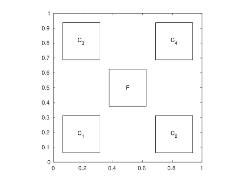
Figure 3. Geometry of the inclusion problem. The four squares in the corners denote the regions appearing in the definition of the diffusion coefficient (49). The central region $F$ is related to the forcing term $f$.

The diffusion coefficient reads

(49) $$a(x,\bm{y})=a_{0}(x)+\sum_{n=1}^{4}\gamma_{n}\chi_{n}y_{n}\qquad\textrm{with }a_{0}\equiv 1.1,$$

where $\left(\gamma_{n}\right)_{n=1}^{4}=\left(0.9,0.6,0.3,0.1\right)$ are constants used to introduce anisotropy in the problem and $\chi_{n}$ is the characteristic function of $C_{n}$, for all $n\in 1,...,4$. The forcing term reads $f(x)\coloneqq 100\chi_{F}$, where $\chi_{F}$ is the characteristic function of $F$. We take $Y_{n}\sim\mathcal{U}(-0.99,0.99)$ for all $n\in 1,...,4$.

The following parameters are chosen for Algorithm 1: Tolerance $\epsilon=2\cdot 10^{-2}$, Dörfler parameter for the collocation points $\theta_{y}=0.5$, Dörfler parameter for mesh elements $\theta_{x}=0.25$, finite element refinement tolerance parameter $\alpha=0.9$ and, as default mesh $\mathcal{T}_{init}$, a quasi-uniform mesh with 2048 triangles and 1089 vertices. The algorithm is driven by the profit with work defined in (12).

The evolution of the estimators, plotted in a log-log scale with respect to the number of degrees of freedom, can be seen in Figure 4. In the first plot, all the computed values of the estimator are plotted. It can be seen how the algorithm alternates between steps of parameter enrichment and mesh refinement. The spikes in the value of the finite element estimator correspond to the parametric enrichment steps, when new collocation points are added to the sparse grid. The finite element solutions corresponding to new collocation points are computed over the default (coarse) mesh $\mathcal{T}_{init}$, which lead to large contributions to the finite element estimator. Observe that when finite element refinement is carried out, the finite element estimator eventually decreases with order $N^{-\frac{1}{2}}$ (where $N$ is the number of degrees of freedom) as a result of the Dörfler marking of the collocation nodes and the order of convergence of the h-adaptive finite element method. Notice how, in the intervals of iterations when finite element refinement is performed, the parametric estimator is updated. While the first update often leads to a considerable change, the following ones have smaller magnitude.

In the second plot, the values of the parametric, finite element and total estimators are plotted only once per iteration of the loop on Algorithm 1. It can be seen that, because of the choice of tolerance (48), the finite element estimator is dominated by the parametric one. Based on the error decay derived in Section 2.3, we expect the finite-element error to dominate the total error up to logarithmic terms. We observe convergence with $N^{-\frac{1}{2}}\log^{4}(N)$, which confirms the theory.

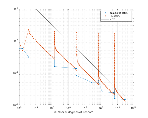
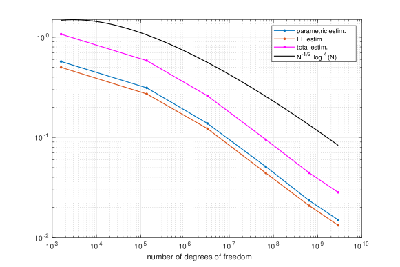
Figure 4. Convergence of the estimators with respect to the number of degrees of freedom for the 4D inclusion problem. Above: detailed evolution of the parametric and of the finite element estimators. Below: value of the estimators plotted once per iteration of Algorithm 1.

References

• [1] Ivo Babuška, Fabio Nobile, and Raul Tempone. A stochastic collocation method for elliptic partial differential equations with random input data. SIAM Journal on Numerical Analysis, 45(3):1005–1034, 2007.
• [2] J. Bäck, F. Nobile, L. Tamellini, and R. Tempone. Stochastic spectral Galerkin and collocation methods for PDEs with random coefficients: a numerical comparison. In J.S. Hesthaven and E.M. Ronquist, editors, Spectral and High Order Methods for Partial Differential Equations, volume 76 of Lecture Notes in Computational Science and Engineering, pages 43–62. Springer, 2011. Selected papers from the ICOSAHOM ’09 conference, June 22-26, Trondheim, Norway.
• [3] Volker Barthelmann, Erich Novak, and Klaus Ritter. High dimensional polynomial interpolation on sparse grids. Advances in Computational Mathematics, 12(4):273–288, 2000.
• [4] Alex Bespalov, Dirk Praetorius, Leonardo Rocchi, and Michele Ruggeri. Convergence of adaptive stochastic galerkin fem. SIAM Journal on Numerical Analysis, 57(5):2359–2382, 2019.
• [5] C. Carstensen, M. Feischl, M. Page, and D. Praetorius. Axioms of adaptivity. Comput. Math. Appl., 67(6):1195–1253, 2014.
• [6] J Manuel Cascon, Christian Kreuzer, Ricardo H Nochetto, and Kunibert G Siebert. Quasi-optimal convergence rate for an adaptive finite element method. SIAM Journal on Numerical Analysis, 46(5):2524–2550, 2008.
• [7] Abdellah Chkifa, Albert Cohen, and Christoph Schwab. High-dimensional adaptive sparse polynomial interpolation and applications to parametric pdes. Foundations of Computational Mathematics, 14(4):601–633, 2014.
• [8] Albert Cohen and Ronald DeVore. Approximation of high-dimensional parametric PDEs. Acta Numer., 24:1–159, 2015.
• [9] Albert Cohen, Ronald DeVore, and Christoph Schwab. Convergence rates of best $N$-term Galerkin approximations for a class of elliptic sPDEs. Found. Comput. Math., 10(6):615–646, 2010.
• [10] J. Dick, F. Y. Kuo, Q. T. Le Gia, D. Nuyens, and C. Schwab. Higher order QMC Petrov-Galerkin discretization for affine parametric operator equations with random field inputs. SIAM J. Numer. Anal., 52(6):2676–2702, 2014.
• [11] Josef Dick, Michael Feischl, and Christoph Schwab. Improved efficiency of a multi-index FEM for computational uncertainty quantification. SIAM J. Numer. Anal., 57(4):1744–1769, 2019.
• [12] Josef Dick, Robert N. Gantner, Quoc T. Le Gia, and Christoph Schwab. Multilevel higher-order quasi-Monte Carlo Bayesian estimation. Math. Models Methods Appl. Sci., 27(5):953–995, 2017.
• [13] Josef Dick, Frances Y. Kuo, Quoc T. Le Gia, Dirk Nuyens, and Christoph Schwab. Higher order QMC Petrov-Galerkin discretization for affine parametric operator equations with random field inputs. SIAM J. Numer. Anal., 52(6):2676–2702, 2014.
• [14] Josef Dick, Frances Y. Kuo, Quoc T. Le Gia, and Christoph Schwab. Multilevel higher order QMC Petrov-Galerkin discretization for affine parametric operator equations. SIAM J. Numer. Anal., 54(4):2541–2568, 2016.
• [15] VK Dzjadyk and VV Ivanov. On asymptotics and estimates for the uniform norms of the lagrange interpolation polynomials corresponding to the chebyshev nodal points. Analysis Mathematica, 9(2):85–97, 1983.
• [16] Martin Eigel, Claude Jeffrey Gittelson, Christoph Schwab, and Elmar Zander. A convergent adaptive stochastic Galerkin finite element method with quasi-optimal spatial meshes. ESAIM Math. Model. Numer. Anal., 49(5):1367–1398, 2015.
• [17] Stefan Funken, Dirk Praetorius, and Philipp Wissgott. Efficient implementation of adaptive p1-fem in matlab. Computational Methods in Applied Mathematics, 11(4):460–490, 2011.
• [18] Diane Guignard and Fabio Nobile. A posteriori error estimation for the stochastic collocation finite element method. SIAM Journal on Numerical Analysis, 56(5):3121–3143, 2018.
• [19] Fabio Nobile, Raúl Tempone, and Clayton G Webster. A sparse grid stochastic collocation method for partial differential equations with random input data. SIAM Journal on Numerical Analysis, 46(5):2309–2345, 2008.
• [20] Grzegorz W Wasilkowski and Henryk Wozniakowski. Explicit cost bounds of algorithms for multivariate tensor product problems. Journal of Complexity, 11(1):1–56, 1995.