A Topological Similarity Measure between Multi-Field Data using Multi-Resolution Reeb Spaces

Abstract

Searching topological similarity between a pair of shapes or data is an important problem in data analysis and visualization. The problem of computing similarity measures using scalar topology has been studied extensively and proven useful in shape and data matching. Even though multi-field (or multivariate) topology-based techniques reveal richer topological features, research on computing similarity measures using multi-field topology is still in its infancy. In the current paper, we propose a novel similarity measure between two piecewise-linear multi-fields based on their multi-resolution Reeb spaces - a newly developed data-structure that captures the topology of a multi-field. Overall, our method consists of two steps: (i) building a multi-resolution Reeb space corresponding to each of the multi-fields and (ii) proposing a similarity measure for a list of matching pairs (of nodes), obtained by comparing the multi-resolution Reeb spaces. We demonstrate an application of the proposed similarity measure by detecting the nuclear scission point in a time-varying multi-field data from computational physics.

Keywords:

Topological Data Analysis, Multi-Field, Reeb Space, Multi-Resolution, JCN, Similarity Measure

1 Introduction

Similarity measures using scalar topology have demonstrated significant applications in shape matching, classification of bio-molecular or protein structures, symmetry detection, periodicity analysis in time-dependant flows, and so on [10, 19, 18, 14]. The design of the similarity algorithms are mostly based on scalar topological data-structures, viz. contour tree, Reeb graph, merge tree, Morse-Smale complex, extremum graph etc.

Since multi-field topology is richer than scalar topology, using multi-field topology one is expected to design more precise similarity measures for better classification of shapes and data. However, this requires generalizations of the existing data-structures for scalar topology to capture multi-field topology. Towards this, in the current paper, we contribute as follows:

• We introduce a novel Multi-resolution Reeb Space (MRS) data-structure to capture the multi-field topology by generalizing the Multi-resolution Reeb Graph (MRG) by Hilaga et al. [10].

• Then, we propose a similarity measure between two MRS structures by generalizing the similarity measure for scalar fields by Hilaga et al. and Zhang et al.[10, 19].

• Finally, we show the effectiveness of our method by detecting the nuclear scission point from our similarity plots for the time-varying multi-field Fermium-$256$ atom dataset as in  [8].

The next section discusses the related works on topological similarity measures. Section 3 provides the necessary background to understand our method. Section 4 and Section 5 describe our algorithms for computing an MRS and computing the proposed similarity measure between two MRSs, respectively. Finally, Section 6 shows an application of our method and concludes with a summary.

2 Related Work

Topological similarity and distance measures between scalar fields have been studied extensively. Beketayev et al.[3] propose an interleaving distance as a distance between merge trees. Bauer et al.[2] propose a stable functional distortion metric for computing distance between two Reeb graphs. Saikia et al. [14] develop an extended branch decomposition graph (eBDG) and identify the repeating topological structure in a scalar data. Thomas et al.[18] propose a multiscale symmetry detection technique using contour clustering. Other work has been done to find similarity between scalar fields by proposing a distance metric between merge trees [3]. Saikia et al.[15] propose a histogram feature descriptor to differentiate between subtrees of a merge tree. Narayanan et al.[11] present a distance measure to compare scalar fields using extremum graphs. Sridharamurthy et al.[16] present an edit distance based method between merge trees for feature visualization in time-varying scalar field data. Among the multi-resolution techniques, the most important ones are by Hilaga et al.[10] - a similarity measure based on multi-resolution Reeb graphs (MRG) and by Zhang et al.[19] - topology matching using multi-resolution dual contour trees. The current paper generalizes these techniques for multi-fields.

However, research on computing topological similarity measures for multi-fields is still at a nascent stage. Recently, Agarwal et al.[1] have proposed a distance metric between two multi-fields based on their fiber-component distributions of and demonstrate its usefulness over scalar-topology. It is worth mentioning few important data-structures for capturing multi-field topology. Carr et al.[4] develop a joint contour net (JCN) for a quantized approximation of the Reeb space. Duke et al.[8] successfully apply the JCN to visualize nuclear scission features in multi-field density data. Chattopadhyay et al.[5, 6] propose a hierarchical multi-dimensional Reeb graph (MDRG) structure equivalent to the Reeb space. These data-structures are useful for the development of the current algorithm.

3 Background

In this section, we describe the necessary background to understand the proposed similarity measure between MRSs. More precisely, we briefly highlight the important tools for capturing the scalar and multi-field topology.

Piecewise-Linear Multi-Fields.

Most of the data in scientific visualization comes as a discrete set of real values at every vertex (grid-point) of a mesh in a volumetric domain. Let us consider the data domain as a compact $m$-dimensional manifold $\mathcal{M}$ and let $\mathbb{M}$ be a triangulation (mesh) of $\mathcal{M}$ whose vertices contain the data values. Let $\mathbf{V}(\mathbb{M})=\{\mathbf{v}_{0},\mathbf{v}_{1},\ldots,\mathbf{v}_{p}\}$ be the set of vertices of $\mathbb{M}$. An $n$-dimensional multi-field data can be described by a vertex map $\hat{\mathbf{f}}=(\hat{f_{1}},\hat{f_{2}},\ldots,\hat{f_{n}}):\mathbf{V}(\mathbb{M})\rightarrow\mathbb{R}^{n}$ which maps each vertex to a $n$-tuple of scalar values. From this discrete map we define a piecewise-linear (PL) multi-field $\mathbf{f}=(f_{1},f_{1},\ldots,f_{n}):\mathbb{M}\rightarrow\mathbb{R}^{n}$ as $\mathbf{f}(\mathbf{x})=\sum_{i=0}^{p}\alpha_{i}\hat{\mathbf{f}}(\mathbf{v}_{i})$ where $\mathbf{x}\in\sigma$ (a simplex of $\mathbb{M}$) has a unique convex combination of its vertices that can be expressed as $\mathbf{x}=\sum_{i=0}^{p}\alpha_{i}\mathbf{v}_{i}$ with $\alpha_{i}\geq 0$ and $\sum_{i=0}^{p}\alpha_{i}=1$. We note, $\mathbf{f}$ is continuous and the restriction of $\mathbf{f}$ over each simplex of $\mathbb{M}$ is linear. In the current paper, we consider the PL multi-field $\mathbf{f}:\mathbb{M}\rightarrow\mathbb{R}^{n}$ with $m\geq n\geq 1$ as our input multi-field. In particular, if $n=1$, $f:\mathbb{M}\rightarrow\mathbb{R}$ is a PL scalar field.

Reeb Space and Reeb Graph.

Given a PL multi-field $\mathbf{f}:\mathbb{M}\rightarrow\mathbb{R}^{n}$ and a range value $\mathbf{c}\in\mathbb{R}^{n}$, the inverse image $\mathbf{f}^{-1}(\mathbf{c})=\{\mathbf{x}\in\mathbb{M}:\mathbf{f}(x)=\mathbf{c}\}$ is called a fiber and a connected component of the fiber is called a fiber-component  [12, 13]. Each fiber-component is an equivalence class obtained by an equivalence relation $\sim$ on $\mathbb{M}$: $\mathbf{x}\sim\mathbf{y}\Leftrightarrow\mathbf{x},\,\mathbf{y}\in\mathbb{M},\;\mathbf{f}(\mathbf{x})=\mathbf{f}(\mathbf{y})=\mathbf{h}$ and $\mathbf{x},\,\mathbf{y}$ belong to the same connected component of $\mathbf{f}^{-1}(\mathbf{h})$. This equivalence relation partitions $\mathbb{M}$ into the set of all equivalence classes or fiber-components. The space $\mathbb{W}_{\mathbf{f}}$ formed by the set of equivalence classes along with the topology induced by a quotient map $q_{\mathbf{f}}:\mathbb{M}\rightarrow\mathbb{W}_{\mathbf{f}}$ is called the Reeb space [9]. The quotient map $q_{\mathbf{f}}$ maps each point of $\mathbb{M}$ to its equivalence class. Geometrically, under some regularity conditions, $\mathbb{W}_{\mathbf{f}}$ is an $n$-dimensional polyhedron.

In particular, for a PL scalar field $f:\mathbb{M}\rightarrow\mathbb{R}$, the fiber $f^{-1}(c)=\{x\in\mathbb{M}:f(x)=c\}$ is known as a level set of the isovalue $c\in\mathbb{R}$ and a connected component of the level set is called a contour instead of fiber-component. Under some regularity conditions, the Reeb space of the scalar field $f:\mathbb{M}\rightarrow\mathbb{R}$ is a $1$-dimensional CW-complex or a graph structure, known as the Reeb graph and is denoted by $\mathcal{RG}_{f}$. Therefore, $\mathcal{RG}_{f}$ consists of a set of nodes and arcs, each arc connecting two of the nodes. Each point of the Reeb graph corresponds to a contour. In particular, the nodes of the Reeb graph correspond to the contours passing through the critical points [7] of $f$ and the arcs connecting the nodes represent the contours which pass through the regular points (not critical!) of $f$.

Multi-Resolution Reeb Graph.

A multi-resolution Reeb graph of a PL scalar field $h:\mathbb{M}\rightarrow\mathbb{R}$, proposed by Hilaga et al. [10], is a data-structure that computes a finite series of Reeb graphs at various levels of data resolutions. In practice, each Reeb graph is obtained by subdividing the data range into a set of $Q=2^{k},\;(k=0,1,\ldots,N-1)$ levels of resolution by a dyadic subdivision (as shown in Figure 1). The domain $\mathbb{M}$ is partitioned into fat (or quantized) contours accordingly and then the Reeb graph at that resolution is obtained by constructing the adjacency graph of the fat contours [10]. The Reeb graphs in an MRG satisfy the following properties: 1. a parent-child relationship is maintained between the nodes of the adjacent Reeb graphs at consecutive levels, 2. by repeating the process of subdivision, when the levels of resolution goes to infinity the MRG converges to the actual Reeb graph of $h$ and 3. a Reeb graph at a particular resolution contains all the information about the coarser resolution Reeb graphs. Figure 1 shows the MRG of the height field of a standing double torus with legs, using $4$ resolutions.

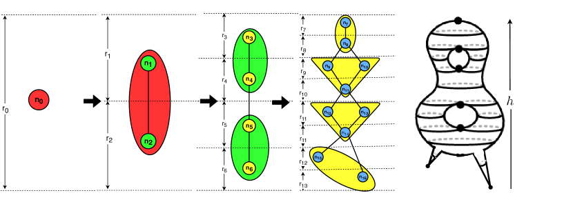
Figure 1: An MRG of the height function $h$ of a standing double torus with legs. The figure shows the MRG with four Reeb graphs at four different resolutions - coarser to finer Reeb graphs are shown from the left to right.

Joint Contour Net.

A Joint Contour Net (JCN) of a PL multi-field $\mathbf{f}=(f_{1},\ldots,f_{n}):\mathbb{M}\rightarrow\mathbb{R}^{n}$, proposed by Carr et al. [4], is a quantized approximation of the Reeb space using a chosen number of quantization levels (or levels of resolution). The data range is first quantized or subdivided into $Q=q_{1}\times q_{2}\times\ldots\times q_{n}$ levels of quantization (here, range of $f_{i}$ is quantized into $q_{i}$ levels, $i=1,2,\ldots,n$), similar as MRG. Thus the range of $\mathbf{f}$ is discretized into a finite set, such as a subset of $\mathbb{Z}^{n}$. In this case, for a quantized range value $\mathbf{h}\in\mathbb{Z}^{n}$, instead of a fiber we obtain a quantized fiber or joint level set, denoted as $\tilde{\mathbf{f}}^{-1}(\mathbf{h})=\{\mathbf{x}\in\mathbb{M}:round(\mathbf{f}(\mathbf{x}))=\mathbf{h}\}$ where the $round$ function is applied on each component. Quantized fibers are not always connected. A connected component of a quantized fiber is called a quantized fiber-component or joint contour. The joint contour net is an adjacency graph of the joint contours or quantized fiber-components. Figure 2(a) shows an example of JCN corresponding to a simulated bivariate dataset. In our method, to compute a multi-resolution Reeb space corresponding to a multi-field, we compute joint contour nets at different resolutions.

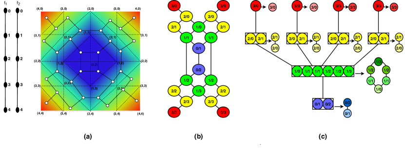
Figure 2: (a) A PL bivariate data over a 2D mesh, (b) JCN at $4\times 4$ resolution, (c) MDRG computed using the algorithm in [6].

Multi Dimensional Reeb Graph.

A Multi Dimensional Reeb Graph (MDRG) of a PL multi-field $f:\mathbb{M}\rightarrow\mathbb{R}^{n}$, proposed by Chattopadhyay et al.[5, 6], is a hierarchical decomposition of the Reeb space (or the corresponding joint contour net) into a set of Reeb graphs in different dimensions. In particular, to construct the MDRG for a PL bivariate field $\mathbf{f}=(f_{1},f_{2}):\mathbb{M}\rightarrow\mathbb{R}^{2}$, we first compute the Reeb graph $\mathcal{RG}_{f_{1}}$ of the field $f_{1}$ (in the first dimension). Now each point $p\in\mathcal{RG}_{f_{1}}$ corresponds to a contour $C_{p}$ of $f_{1}$. We restrict function $f_{2}$ (second dimension) on $C_{p}$ and define the restricted function $\widetilde{f}_{2}^{p}=f_{2}|_{C_{p}}$. Then for the second dimension, we compute Reeb graphs $\mathcal{RG}_{\widetilde{f}_{2}^{p}}$ for each of these restricted functions $\widetilde{f}_{2}^{p}$. Thus MDRG of $f$, denoted by $\mathrm{MDRG}_{f}$, can be defined as: $\mathrm{MDRG}_{f}=\{(p_{1},p_{2}):p_{1}\in\mathcal{RG}_{f_{1}},p_{2}\in\mathcal{RG}_{\widetilde{f}_{2}^{p_{1}}}\}$. The definition can be extended for any PL multi-field $\mathbf{f}:\mathbb{M}\rightarrow\mathbb{R}^{n}$ with $m\geq n>2$. Fig. 2(b) shows an example of a quantized Reeb space or JCN for a PL bivariate field (in Fig. 2(a)) and Fig. 2(c) shows its MDRG.

4 Multi-Resolution Extension of Reeb Space

In this section, we develop a new multi-resolution Reeb space structure that captures the topology of a PL multi-field data at different resolutions, similar as MRG of a PL scalar field [10]. The Reeb space at a particular resolution is approximated by the JCN. The idea is to develop a series of JCNs at various resolutions.

4.1 Overview

Let $\mathbf{f}=(f_{1},f_{2},\ldots,f_{n}):\mathbb{M}\rightarrow\mathbb{R}^{n}$ be a PL multi-field and $\mathrm{JCN}_{\mathbf{f}}(\mathbf{q})$ denote the JCN of $\mathbf{f}$ with parameter-vector $\mathbf{q}=(q_{1},q_{2},\ldots,q_{n})$, each parameter $q_{i}$ being the levels of resolution of the component field $f_{i}$ for $i\in\{1,2,\ldots,n\}$. Thus, using $\mathbf{q}$, we obtain an approximated Reeb space $\mathrm{JCN}_{\mathbf{f}}(\mathbf{q})$ with $Q=q_{1}\times q_{2}\times\ldots\times q_{n}$ levels of resolution of the multi-field $\mathbf{f}$. Now to construct a multi-resolution Reeb space, for simplicity, we consider a finite sequence $\{\mathbf{q}^{(k)}=(2^{k},2^{k},\ldots,2^{k}):k=0,1,\ldots,N-1\}$ of $N\,(\geq 1)$ increasing levels of resolution of $\mathbf{f}$. Corresponding to this sequence of resolutions, we obtain a sequence $\left\{\mathrm{JCN}_{\mathbf{f}}(\mathbf{q}^{(k)}):k=0,1,\ldots,N-1\right\}$ of $N$ approximated Reeb spaces that defines a Multi-resolution Reeb Space (MRS) of $\mathbf{f}$ with $N$ levels of resolution and is denoted by $\mathrm{MRS}_{\mathbf{f},\,N}$. Moreover, $\mathrm{JCN}_{\mathbf{f}}(\mathbf{q}^{(k)})$ or $\mathrm{JCN}_{\mathbf{f},\,k}$ (in short) for $k=0,1,\ldots,N-1$ of the MRS satisfy the following properties:

1. There are parent-child relationships between the nodes of adjacent resolutions, i.e between the nodes in $\mathrm{JCN}_{\mathbf{f},\,k}$ and $\mathrm{JCN}_{\mathbf{f},\,k+1}$. For example, in Figure 3, node $n_{0}$ of the JCN in (d) is the parent of the nodes $\{n_{1},n_{2},n_{3},n_{4},n_{5},n_{6}\}$ of the JCN in (e).

2. Note that when the levels of resolution goes to infinity the JCN graph converges to the Reeb space of $\mathbf{f}$, i.e. $\mathrm{JCN}_{\mathbf{f},\,k}$ converges to the Reeb space $\mathbb{W}_{\mathbf{f}}$ as $k\rightarrow\infty$ (see [6] for details). In otherwords, we can say the multi-resolution Reeb space $\mathrm{MRS}_{\mathbf{f},\,N}$ converges to $\mathbb{W}_{\mathbf{f}}$ as the levels of resolution $N$ tends to $\infty$.

3. A JCN of a certain resolution in $\mathrm{MRS}_{\mathbf{f},\,N}$ implicitly contains all the information of the JCNs of coarser resolutions, i.e. $\mathrm{JCN}_{\mathbf{f},\,k}$ contains all the information of $\mathrm{JCN}_{\mathbf{f},\,0},\,\mathrm{JCN}_{\mathbf{f},\,1},\,\ldots,\mathrm{JCN}_{\mathbf{f},\,k-1}$. Once a JCN of a certain resolution is constructed, the coarser resolution JCN can be constructed by grouping the adjacent nodes in same coarser range interval, as shown in Figure 3.

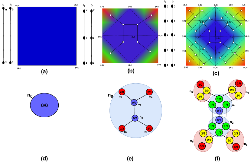
Figure 3: Multi-resolution Reeb Space corresponding to a PL bivariate data: (ring, height). (a) Each component field is quantized into one level, and the corresponding JCN in (d) consists of only one node $n_{0}$. (b) Each component field is quantized into two levels and the corresponding JCN is shown is (e). (c) Each component field is quantized into four levels, and the corresponding JCN is shown in (f). Parent-child relationships between the nodes of JCNs in consecutive resolutions are shown, e.g. $n_{0}$ is parent of $\{n_{1},n_{2},n_{3},n_{4},n_{5},n_{6}\}$.

4.2 Construction of the Multi-Resolution Reeb Space

Consider the parameter vector $\mathbf{q}^{(N-1)}=(2^{N-1},2^{N-1},\ldots,2^{N-1})$ of (dyadic) levels of resolutions corresponding to PL multi-field $\mathbf{f}=(f_{1},f_{2},\ldots,f_{n})$ where $N\,(\geq 1)$ is an integer. Then the JCN of $\mathbf{f}$, using $\mathbf{q}^{(N-1)}$, can be constructed using the algorithm described by Carr et al. [4] and is denoted by $\mathrm{JCN}_{\mathbf{f}}(\mathbf{q}^{(N-1)})$ or $\mathrm{JCN}_{\mathbf{f},\,N-1}$. To construct the multi-resolution Reeb space $\mathrm{MRS}_{\mathbf{f},N}$, we start with $\mathrm{JCN}_{\mathbf{f},\,N-1}$ and construct its coarser resolution Reeb spaces, sequentially, by merging each pair of consecutive range intervals and grouping the adjacent nodes in the corresponding intervals. This is similar to the construction of MRG by Hilaga et al.[10]. Algorithm 1 outlines the method for constructing a coarser resolution Reeb space $\mathrm{JCN}_{\mathbf{f},\,k-1}$ from the finer resolution Reeb space $\mathrm{JCN}_{\mathbf{f},\,k}$. Let $R_{\mathbf{f}}=[f_{1}^{\min},\,f_{1}^{\max}]\times[f_{2}^{\min},\,f_{2}^{\max}]\times\ldots\times[f_{n}^{\min},\,f_{n}^{\max}]$ be the $n$-dimensional range interval of the multi-field $\mathbf{f}$ where $f_{i}^{\min}=\displaystyle\min_{\mathbf{x}\in\mathbb{M}}f_{i}(\mathbf{x})$ and $f_{i}^{\max}=\displaystyle\max_{\mathbf{x}\in\mathbb{M}}f_{i}(\mathbf{x})$ for $i=1,2,\ldots,n$. The range $[f_{i}^{\min},\,f_{i}^{\max}]$ of the component field $f_{i}$ (for $i=1,2,\ldots,n$) is subdivided into $q=2^{k}$ ($k\in\mathbb{N}:$ set of natural numbers) dyadic levels of resolution or sub-intervals: $r_{0}^{(i)}=[x_{0}^{(i)},\,x_{1}^{(i)}),\,r_{1}^{(i)}=[x_{1}^{(i)},\,x_{2}^{(i)}),\ldots,r_{q-1}^{(i)}=[x_{q-1}^{(i)},\,x_{q}^{(i)}]$, where $x_{0}^{(i)}=f_{i}^{\min}$ and $x_{q}^{(i)}=f_{i}^{\max}$ ($i=1,2,\ldots,n$). Thus the range $R_{\mathbf{f}}$ is subdivided into $Q=q\times q\times\ldots\times q$ ($n$ times) dyadic levels of resolution or sub-intervals, denoted by $r_{i_{1}i_{2}\ldots i_{n}}=r_{i_{1}}^{(1)}\times r_{i_{2}}^{(2)}\times\ldots\times r_{i_{n}}^{(n)}$ (where $i_{1},i_{2},\ldots,i_{n}=0,1,\ldots,q-1$). For computing the coarser level Reeb space $\mathrm{JCN}_{\mathbf{f},\,k-1}$ (where $k\geq 1$) we merge the adjacent levels of $\mathrm{JCN}_{\mathbf{f},\,k}$ (in pairs) and obtain the coarser sub-intervals as $R_{i_{1}i_{2}\ldots i_{n}}=\mathrm{merge}(r_{2i_{1}}^{(1)},r_{2i_{1}+1}^{(1)})\times\mathrm{merge}(r_{2i_{2}}^{(2)},r_{2i_{2}+1}^{(2)})\times\ldots\times\mathrm{merge}(r_{2i_{n}}^{(n)},r_{2i_{n}+1}^{(n)})$ (for $i_{1},i_{2},\ldots,i_{n}=0,1,\ldots,\frac{q}{2}-1$). So the levels of resolution of $\mathrm{JCN}_{\mathbf{f},\,k-1}$ reduces to $\tilde{Q}=\frac{q}{2}\times\frac{q}{2}\times\ldots\times\frac{q}{2}$. We construct a Union-Find structure UF [17] from the adjacency of the nodes of $\mathrm{JCN}_{\mathbf{f},\,k}$ with ranges in $R_{i_{1}i_{2}\ldots i_{n}}$. Each connected component of UF becomes a node of the coarser Reeb space $\mathrm{JCN}_{\mathbf{f},\,k-1}$ and the adjacencies of these new nodes are determined by the adjacencies of the components in $\mathrm{JCN}_{\mathbf{f},\,k}$.

Algorithm 1 CreateCoarserReebSpace

Input: $\mathrm{JCN}_{\mathbf{f},\,k}$
Output: $\mathrm{JCN}_{\mathbf{f},\,k-1}$

1:  for $i_{1}=0$ to $\frac{q}{2}-1$ do

2:     for $i_{2}=0$ to $\frac{q}{2}-1$ do

3:        $\ddots$

4:        for $i_{n}=0$ to $\frac{q}{2}-1$ do

5:           % RANGE MERGING FOR COARSER RESOLUTION

6:           $R_{i_{1}i_{2}\ldots i_{n}}=\mathrm{merge}(r_{2i_{1}}^{(1)},r_{2i_{1}+1}^{(1)})\times\mathrm{merge}(r_{2i_{2}}^{(2)},r_{2i_{2}+1}^{(2)})\times\ldots\times\mathrm{merge}(r_{2i_{n}}^{(n)},r_{2i_{n}+1}^{(n)})$

7:           Create Union-Find Structure UF for the nodes of $\mathrm{JCN}_{\mathbf{f},k}$ in range $R_{i_{1}i_{2}\ldots i_{n}}$

8:           % CREATING NODES OF COARSER JCN

9:           for  each component $C_{j}$ in UF do

10:              Create a node $n_{C_{j}}$ in $\mathrm{JCN}_{\mathbf{f},\,k-1}$

11:              Map node-ids and field-values of the finer JCN

12:              Set node $n_{C_{j}}$ as the parent for the nodes in $C_{j}$

13:           end for

14:        end for

15:     end for

16:     $\udots$

17:  end for

18:  % ADDING EDGES IN COARSER JCN

19:  for  each edge $e_{1}e_{2}$ in $\mathrm{JCN}_{\mathbf{f},\,k}$ do

20:     if $e_{1},e_{2}\in$ components $C_{j}\neq C_{l}$ and $\mathbf{f}(e_{1})\neq\mathbf{f}(e_{2})$ then

21:        Add edge $e(n_{C_{j}},n_{C_{l}})$ in $\mathrm{JCN}_{\mathbf{f},\,k-1}$ if not already present

22:     end if

23:  end for

24:  return  $\mathrm{JCN}_{\mathbf{f},\,k-1}$

Figure 3 illustrates an MRS for a simple bivariate data in a 2D box domain with $3$ levels of resolution. The construction of the MRS starts with the construction of the Reeb space with $Q=2^{2}\times 2^{2}$ levels at the finest resolution.

4.3 Node Attributes for Similarity Measure

To obtain a quantitative similarity measure between two multi-resolution Reeb spaces, we associate several attributes to the nodes of the MRS that quantify different topological and geometrical properties of the multi-field data, similar as in  [10, 19]. The attribute set corresponding to a node $\mathbf{n}$, denoted by $\widetilde{\mathbf{n}}$, is defined as $\widetilde{\mathbf{n}}=\{\mathcal{V}(\mathbf{n}),\mathcal{R}(\mathbf{n}),\mathcal{B}_{0}(\mathbf{n}),\mathcal{D}(\mathbf{n})\}$ where $\mathcal{V}(\mathbf{n})=\frac{\text{Volume}(\mathbf{n})}{\text{Total Volume}(\mathbb{M})}$ is the normalized volume of the node $\mathbf{n}$, $\mathcal{R}(\mathbf{n})=\frac{\text{measure}(\text{range}(\mathbf{n}))}{\text{measure}(\text{range}(\mathbf{f}))}$ is the normalized range, $\mathcal{B}_{0}(\mathbf{n})$ is the number of components of the joint level set corresponding to $\mathbf{n}$ and $\mathcal{D}(\mathbf{n})$ is the degree of $\mathbf{n}$ in the corresponding JCN.

5 A Similarity Measure between MRSs

Let $\mathrm{MRS}_{\mathbf{f},\,N}$ and $\mathrm{MRS}_{\mathbf{g},\,N}$ be two multi-resolution Reeb spaces with same levels of resolution (here, $N$) corresponding to two PL multi-fields $\mathbf{f}$ and $\mathbf{g}$, respectively. Our method of computing the similarity measure between two MRSs has two steps: 1. Creating a list of matching pairs from the nodes of the respective MRSs and 2. Computing the similarity measure between the MRSs by defining a similarity between the nodes of a matched pair. We describe these steps in the following subsections.

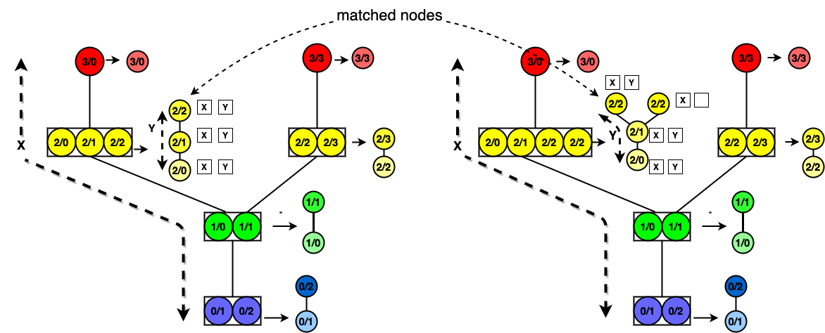
Figure 4: Label propagation is demonstrated for a matching pair in two MDRGs. For a bivariate field, two lists of labels need to be maintained.

5.1 Creating Matching Pairs

To create the list of matching pairs between two multi-resolution Reeb spaces, denoted by $\mathrm{MPAIR}$, we search from the coarser to the finer resolution Reeb spaces. Nodes $\mathbf{m}\in\mathrm{MRS}_{\mathbf{f},\,N}$ and $\mathbf{n}\in\mathrm{MRS}_{\mathbf{g},\,N}$ form a matching pair $(\mathbf{m},\mathbf{n})\in\mathrm{MPAIR}$ if they satisfy the following matching rules (generalizing the rules in [10, 19]):

1. $\mathbf{m}\in\mathrm{MRS}_{\mathbf{f},\,N}$ and $\mathbf{n}\in\mathrm{MRS}_{\mathbf{g},\,N}$ do not belong to any other matched pair,

2. $\mathbf{m}$ and $\mathbf{n}$ belong to the Reeb space of same resolution and both have the same range level,

3. Parent $p(\mathbf{m})$ of $\mathbf{m}$ and parent $p(\mathbf{n})$ of $\mathbf{n}$ must have been matched, i.e. $(p(\mathbf{m}),p(\mathbf{n}))$ is already a matching pair, except for the nodes in the coarsest resolution,

4. $\mathbf{m}$ and $\mathbf{n}$ must be topologically consistent. Unlike computing consistency using Reeb graphs in [10], here we consider the MDRGs of the corresponding Reeb spaces. That is, $\mathbf{m}$ and $\mathbf{n}$ should be in the same branches of the respective MDRGs as their matched siblings in all dimensions. In particular, for a bivariate field, to satisfy the topological consistency in each dimension, two lists of labels are maintained corresponding to each node. Once two nodes are matched and labeled, their siblings in the same branch of the MDRG get the same labels (in each dimension), as shown in Figure 4.

Creating the list $\mathrm{MPAIR}$ of matching pairs between two MRSs is outlined in Algorithm 2.

Algorithm 2 CreatingMatchingPairs

Input: Multi-resolution Reeb spaces $\mathrm{MRS}_{\mathbf{f},\,N},\,\mathrm{MRS}_{\mathbf{g},\,N}$
Output: $\mathrm{MPAIR}$ - list of matched pairs

1:  for $k=0,1,\ldots,N-1$ do

2:     Add all the nodes of $\mathrm{JCN}_{\mathbf{f},\,k}$ to a priority queue $\mathbf{Q}$ where the priority of a node is set as its volume attribute.

3:     while $\mathbf{Q}$ is not empty do

4:        $\mathbf{m}\leftarrow\mathrm{Pop}(\mathbf{Q})$. Search for its best matching pair $\mathbf{n}\in\mathrm{JCN}_{\mathbf{g},\,k}$, satisfying the matching rules (i)-(iv).

5:        if $\mathbf{n}$ is found then

6:           $\mathrm{MPAIR}\leftarrow\mathrm{Add}(\{(\mathbf{m},\mathbf{n}),k\})$

7:        end if

8:     end while

9:  end for

10:  return  $\mathrm{MPAIR}$

5.2 Similarity Calculation

Following Zhang et al.[19], first we define a real-valued similarity function $\varphi$ for each matched pair $(\mathbf{m},\mathbf{n})\in\mathrm{MPAIR}$ as:

$$\varphi(\mathbf{m},\mathbf{n})=\omega_{1}\widetilde{\varphi}(\mathcal{V}(\mathbf{m}),\mathcal{V}(\mathbf{n}))+\omega_{2}\widetilde{\varphi}(\mathcal{R}(\mathbf{m}),\mathcal{R}(\mathbf{n}))+$$ (1)

$$\omega_{3}\widetilde{\varphi}(\mathcal{B}_{0}(\mathbf{m}),\mathcal{B}_{0}(\mathbf{n}))+\omega_{4}\widetilde{\varphi}(\mathcal{D}(\mathbf{m}),\mathcal{D}_{0}(\mathbf{n}))$$

where the weights $\omega_{i}$ satisfy $0\leq\omega_{i}\leq 1$ for $i=1,2,3,4$ and $\sum_{i=1}^{4}\omega_{i}=1$ and the function $\widetilde{\varphi}:\mathbb{R}^{+}\times\mathbb{R}^{+}\rightarrow\mathbb{R}^{+}$ is defined as $\widetilde{\varphi}(r_{1},r_{2})=\frac{\min(r_{1},r_{2})}{\max(r_{1},r_{2})}$. Thus, we have $0\leq\varphi(\mathbf{m},\mathbf{n})\leq\varphi(\mathbf{m},\mathbf{m})=\varphi(\mathbf{n},\mathbf{n})=1$.

Next, we define the similarity function $\Phi$ between two $k$-th resolution JCNs $\mathrm{JCN}_{\mathbf{f},k}$ and $\mathrm{JCN}_{\mathbf{g},k}$, by the weighed sum of the similarities for all pairs $(\mathbf{m}_{i},\mathbf{n}_{i})\in\mathrm{MPAIR}$ with $\mathbf{m}_{i}\in\mathrm{JCN}_{\mathbf{f},k}$ and $\mathbf{n}_{i}\in\mathrm{JCN}_{\mathbf{g},k}$, as

$$\Phi(\mathrm{JCN}_{\mathbf{f},k},\mathrm{JCN}_{\mathbf{g},k})=\sum_{i=1}^{s}\frac{\mathcal{V}(\mathbf{m}_{i})+\mathcal{V}(\mathbf{n}_{i})}{2}\varphi(\mathbf{m}_{i},\mathbf{n}_{i})$$ (2)

where $s$ is the total number of such pairs. Finally, we define the similarity $\overline{\Phi}$ between two MRSs $\mathrm{MRS}_{\mathbf{f},N}$ and $\mathrm{MRS}_{\mathbf{g},N}$ as

$$\overline{\Phi}(\mathrm{MRS}_{\mathbf{f},N},\mathrm{MRS}_{\mathbf{g},N})=\frac{1}{N}\sum_{k=0}^{N-1}\Phi(\mathrm{JCN}_{\mathbf{f},k},\mathrm{JCN}_{\mathbf{g},k})$$ (3)

We note, $0\leq\overline{\Phi}(\mathrm{MRS}_{\mathbf{f},N},\mathrm{MRS}_{\mathbf{g},N})\leq\overline{\Phi}(\mathrm{MRS}_{\mathbf{f},N},\mathrm{MRS}_{\mathbf{f},N})=1$.

6 Implementation and Application

We implement our algorithm for computing the similarity between two multi-resolution Reeb spaces under the JCN implementation framework [4]. As an application of our tool, we consider the time-varying Fermium-$256$ atom dataset as described by Duke et al. [8]. The dataset is defined on a $19\times 19\times 19$ sized grid and consists of proton and neutron densities for $40$ regularly spaced time-steps. Figure 5 shows the similarity plots by pairwise comparison of the datasets at consecutive time-stamps - for $4$ different resolutions and $4$ attributes. From the plots, we see a major topological event at site $26$ which is the nuclear scission, as described by Duke et al.[8].

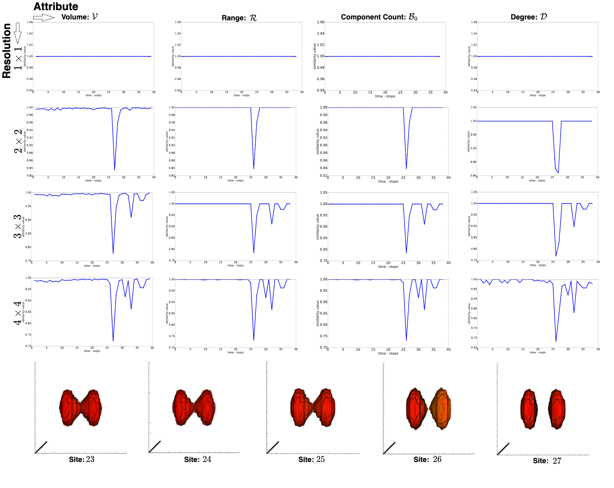
Figure 5: Top-four rows: Similarity plots for time-varying Fermium atom data. Each row shows the metric plots using multi-resolution Reeb spaces with $4$ different attributes. Each column shows the metric plots using multi-resolution Reeb spaces of $4$ different resolutions. Bottom-row: Nucleus is visualized at Sites: $23-27$, the split happens at Site $26$ - corresponding to the ‘lowest’ dip in the plots.

7 Conclusion

In this article, we propose a novel Reeb space based method for measuring the topological similarity between two multi-field data. To compute the similarity measure, we develop a multi-resolution Reeb space data-structure which converges to the actual Reeb space as the levels of resolution goes to infinity. We show effectiveness of our method in the application of detecting nuclear scission point in a time-varying multi-field data.

References

- [1] T. Agarwal, A. Chattopadhyay, and V. Natarajan. Topological Feature Search in Time-Varying Multifield Data. TopoInVis 2019, Nyköping, Sweden, preprint arXiv:1911.00687, 2019.
- [2] U. Bauer, X. Ge, and Y. Wang. Measuring Distance between Reeb graphs. In Proceedings of the thirtieth annual symposium on Computational geometry, page 464. ACM, 2014.
- [3] K. Beketayev, D. Yeliussizov, D. Morozov, G. H. Weber, and B. Hamann. Measuring the Distance between Merge Trees. In Topological Methods in Data Analysis and Visualization III, pages 151–165. Springer, 2014.
- [4] H. Carr and D. Duke. Joint Contour Nets. IEEE Transactions on Visualization and Computer Graphics, 20(8):1100–1113, Aug 2014.
- [5] A. Chattopadhyay, H. Carr, D. Duke, and Z. Geng. Extracting Jacobi Structures in Reeb Spaces. In N. Elmqvist, M. Hlawitschka, and J. Kennedy, editors, EuroVis - Short Papers, pages 1–4. The Eurographics Association, 2014.
- [6] A. Chattopadhyay, H. Carr, D. Duke, Z. Geng, and O. Saeki. Multivariate topology simplification. Computational Geometry: Theory and Application, 58:1–24, 2016.
- [7] K. Cole-McLaughlin, H. Edelsbrunner, J. Harer, V. Natarajan, and V. Pascucci. Loops in Reeb Graphs of 2-Manifolds. In Proceedings of the Nineteenth Annual Symposium on Computational Geometry, SCG ’03, page 344–350, New York, NY, USA, 2003. Association for Computing Machinery.
- [8] D. Duke, H. Carr, N. Schunck, H. A. Nam, and A. Staszczak. Visualizing Nuclear Scission Through a Multifield Extension of Topological Analysis. IEEE Transactions on Visualization and Computer Graphics, 18(12):2033–2040, 2012.
- [9] H. Edelsbrunner, J. Harer, and A. K. Patel. Reeb Spaces of Piecewise Linear Mappings. In SoCG, pages 242–250, 2008.
- [10] M. Hilaga, Y. Shinagawa, T. Kohmura, and T. L. Kunii. Topology Matching for Fully Automatic Similarity Estimation of 3D Shapes. In Proceedings of the 28th annual conference on Computer graphics and interactive techniques, pages 203–212. ACM, 2001.
- [11] V. Narayanan, D. M. Thomas, and V. Natarajan. Distance between Extremum Graphs. In 2015 IEEE Pacific Visualization Symposium (PacificVis), pages 263–270. IEEE, 2015.
- [12] O. Saeki. Topology of Singular Fibers of Differentiable Maps. Springer, 2004.
- [13] O. Saeki, S. Takahashi, D. Sakurai, H.-Y. Wu, K. Kikuchi, H. Carr, D. Duke, and T. Yamamoto. Visualizing Multivariate Data Using Singularity Theory, volume 1 of Mathematics for Industry, chapter The Impact of Applications on Mathematics, pages 51–65. Springer Japan, 2014.
- [14] H. Saikia, H.-P. Seidel, and T. Weinkauf. Extended Branch Decomposition Graphs: Structural Comparison of Scalar Data. Computer Graphics Forum, 33(3):41–50, 2014.
- [15] H. Saikia, H.-P. Seidel, and T. Weinkauf. Fast Similarity Search in Scalar Fields using Merging Histograms. In Topological Methods in Data Analysis and Visualization, pages 121–134. Springer, 2015.
- [16] R. Sridharamurthy, T. B. Masood, A. Kamakshidasan, and V. Natarajan. Edit Distance between Merge Trees. IEEE Transactions on Visualization and Computer Graphics, 26(3):1518–1531, 2020.
- [17] R. E. Tarjan. Efficiency of a Good But Not Linear Set Union Algorithm. J. ACM, 22(2):215–225, Apr. 1975.
- [18] D. M. Thomas and V. Natarajan. Multiscale symmetry detection in scalar fields by clustering contours. IEEE Trans. Visualization and Computer Graphics, 20(12):2427–2436, 2014.
- [19] X. Zhang, Marcos, C. L. Bajaj, and N. Baker. Fast Matching of Volumetric Functions Using Multi-resolution Dual Contour Trees. 2004.