Models of decaying FIMP Dark Matter: potential links with the Neutrino Sector

Abstract

The absolute stability of a dark matter (DM) particle is not a binding requirement. Here we suggest a few scenarios where the DM particle is liable to decay via extremely feeble interactions. This can happen via inexplicably small Yukawa couplings in the simplest conjectures. After setting down such a model, we go beyond it, thus treading onto scenarios where the spontaneous breakdown of some gauged $U(1)$ symmetry may lead to intermediate scales, and suitably suppressed effective operators which allow the DM particle to decay slowly. The constraints from particle physics as well as cosmology are taken into account in each case. The last and more involved scenario, studied in detail, suggest a link between the model parameters that govern neutrino physics on one side, and the dynamics of a quasi-stable DM particle on the other.

1 Introduction

Dark matter (DM) is an undeniable component of the universe today, playing a fundamental role in structure formation and in explaining galactic rotation curves and other astrophysical and cosmological observations Ade:2015xua . Assuming a $\mathbb{Z}_{2}$ symmetry is a frequently adopted practice in ensuring a stable particle in the elementary particle spectrum, which can account for dark matter (DM) in our universe. In special cases like the minimal supersymmetric standard model (MSSM) lepton and baryon number conservation and stability of the proton may (though somewhat grudgingly) be taken as facts supported by experiments. In general, however, such broader theoretical motivation for $\mathbb{Z}_{2}$ symmetries are difficult to find. Furthermore, global symmetries are not likely to be respected by quantum gravity Banks:2010zn ; Mambrini:2015sia ; Harlow:2018jwu . Thus even a scenario that is $\mathbb{Z}_{2}$-symmetric at low energy may permit very small violation of the discrete symmetry, when one takes its UV-completion into account.

On the other hand, dark matter does not have to be absolutely stable. Indeed it is possible that the dark matter candidate(s) has extremely slow decays, with a lifetime much longer than the age of the Universe, due to correspondingly small couplings, whose smallness is protected in spite of radiative corrections. Here we wish to illustrate such a scenario, devoid of any discrete symmetry and consisting of a very long-lived dark matter particle. For these very small DM couplings, the most typical mechanisms for dark matter production are the freeze-in Hall:2009bx ; Bernal:2017kxu and SuperWIMP mechanisms Covi:1999ty ; Feng:2003xh , which rely on the generation of the DM particles from a mother particle in thermal equilibrium. In our model we will therefore also have additional charged states, which can be in equilibrium with the SM, produce DM and mediate interactions between the DM and the dark sector.

The approach to construct a model with decaying dark matter, followed in this work, consists of three levels with increasing complexity of the model as well as naturality. We will consider in all cases a spin-1/2 DM candidate which can decay only via very small Yukawa interactions or higher-dimensional operators.

As the first case, we consider a model with minimal field content and renormalizable Yukawa couplings driving DM decay. It should be remembered here that the Yukawas in the standard model (SM) vary over some five orders of magnitude, without any fundamental principle explaining them. Though this is somewhat dissatisfying, a redeeming feature is that these couplings are ‘technically natural’ tHooft:1979rat , since their radiative corrections, are always proportional to the tree-level Yukawa couplings with additional coefficients $\leq 1$. Emboldened by this, we construct a scenario with not only new Yukawas of even smaller magnitude than those in the SM, but also some gauge-invariant fermion masses, which are all shown to be stable against radiative corrections for certain ranges of values of the parameters. This again makes the added terms ‘technically natural’.

This ‘simple’ scenario leads not only to a dark matter candidate consistent with relic density from freeze-in, but also to an entire spectrum consistent with neutrino masses and mixing, FCNC, lepton universality, Higgs decay data etc. We introduce in the model three SM singlet Majorana fermions, the lightest of which serve as the dark matter candidate, bringing this model within the class of decaying sterile neutrino DM models similar to the $\nu$SM Asaka:2005pn ; Shaposhnikov:2006xi ; Shaposhnikov:2006nn .

In addition a vector-like doublet $F$ has been considered, whose decay is responsible for the freeze-in production of the dark matter, as in Arcadi:2013aba ; Arcadi:2014tsa . The dark matter decays to three fermions via Yukawa interaction with the SM Higgs, the strength of which needs to be extremely small ($\leq 10^{-20}$) in order to be consistent with DM decay observables. The smallness of this interaction strength, of a degree much more severe than what is seen in the SM, is inexplicable from the premises of the model, even if radiatively stable.

To take care of the above issue, a slightly expanded scenario is proposed in the next step. We add a local $U(1)$ symmetry that is broken spontaneously with the help of a scalar $\phi$ at an intermediate scale around $10^{8}$ GeV. All the dark sector fields, $F,\psi$(DM) and $\phi$, are charged under this new gauge symmetry. One can write down dimension 5-and-6 operators, invariant under the SM gauge group as well as the new $U(1)$, suppressed by the Planck scale. Once the $U(1)$ symmetry is broken spontaneously, these higher-dimensional operators lead to mixing and highly suppressed interaction terms between the dark sector fermions and the SM leptons. These not only generate the tiny Yukawa couplings that causes the DM to decay but also the interactions and the decay amplitudes for the $F$ to decay into DM with the level of smallness consistent with freeze-in production.

Finally, we upgrade the $U(1)$ gauge symmetry to $U(1)_{L_{\mu}-L_{\tau}}$ so as to establish a direct connection between DM and the leptonic sector. It is well-known that $U(1)_{L_{\mu}-L_{\tau}}$ can provide an explanation for the large neutrino mixing in the $\mu-\tau$ sector Baek:2001kca ; Lam:2001fb ; Ma:2001md . Moreover quite a number of DM models have already been put forward in the context of $U(1)_{L_{\mu}-L_{\tau}}$ Baek:2008nz ; Baek:2015fea ; Patra:2016shz ; Altmannshofer:2016jzy ; Biswas:2016yjr ; Biswas:2016yan ; Biswas:2017ait but often in different contexts than in the present paper. This scenario has all the advantages of the earlier model along with the DM-neutrino connection which provides it some additional merit. Thus we present the phenomenology of this model in greater details. Here the presence of the higher-dimensional terms in the neutrino mass matrix allow us to obey the PLANCK bound on sum of the light neutrino masses unlike the simple case with only renormalizable terms Asai:2017ryy ; Asai:2018ocx . Moreover we have observable predictions for neutrinoless double-beta decay $0\nu\beta\beta$.

The last-mentioned ‘gauged scenario’ may also be motivated from the angle of UV-completion. On the one hand, such a symmetry is attractive from a neutrino physics point of view. On the other, such a $U(1)$ may be the result of the breaking chain of a gauge group corresponding to a grand unified theory (GUT) at an intermediate scale QUIROS1987461 ; PhysRevLett.60.1817 . Thus both a quasi-stable DM and the physics of lepton sector can be linked to a GUT scenario.

The paper is organized as follows. In section 2 we discuss the $U(1)$-model followed by a short discussion of the renormalizable model. In section 3 we discuss the $L_{\mu}-L_{\tau}$ scenario in details. We summarize and conclude in section 4.

2 Simplified Models

2.1 Model 1

We first consider a model with three generations of RH fermions and one $SU(2)_{L}$ doublet vectorlike fermion in addition to the the SM particle content without imposing any additional symmetries. The newly added particles and their respective charges is shown in tab. 1 where three generations of singlet fermions $N_{R,1},N_{R,2},N_{R,3}$ are collectively denoted as $N_{R,i}$.

Fields	$SU(3)_{c}$	$SU(2)_{L}$	$U(1)_{Y}$
$N_{R,i}$	1	1	0
$F=\left(\begin{matrix}F^{0}\\ F^{-}\end{matrix}\right)$	1	2	-1/2
$\overline{F}=\left(\begin{matrix}\overline{F}^{0}\\ F^{+}\end{matrix}\right)$	1	$\overline{2}$	1/2

Table 1: The quantum numbers of the new fields in Model 1.

The renormalizable Lagrangian comprised of the newly added fields is,

$$\mathcal{L}= \overline{N}_{R,i}i\mathchoice{\ooalign{$\hfil\displaystyle\mkern 0.0mu/\hfil$\crcr$\displaystyle D$}}{\ooalign{$\hfil\textstyle\mkern 0.0mu/\hfil$\crcr$\textstyle D$}}{\ooalign{$\hfil\scriptstyle\mkern 0.0mu/\hfil$\crcr$\scriptstyle D$}}{\ooalign{$\hfil\scriptscriptstyle\mkern 0.0mu/\hfil$\crcr$\scriptscriptstyle D$}}\,N_{R,i}+\overline{F}i\mathchoice{\ooalign{$\hfil\displaystyle\mkern 0.0mu/\hfil$\crcr$\displaystyle D$}}{\ooalign{$\hfil\textstyle\mkern 0.0mu/\hfil$\crcr$\textstyle D$}}{\ooalign{$\hfil\scriptstyle\mkern 0.0mu/\hfil$\crcr$\scriptstyle D$}}{\ooalign{$\hfil\scriptscriptstyle\mkern 0.0mu/\hfil$\crcr$\scriptscriptstyle D$}}\,F-M_{N,i}\overline{N^{c}_{R,i}}N_{R,i}-M_{F}\overline{F}F-M_{l_{i}F}\left(\overline{L_{L,i}}F_{R}+\overline{F_{R}}L_{L,i}\right)$$

$$- \left(Y_{N_{i}}\overline{L_{L}}H^{c}N_{R,i}+Y^{\dagger}_{N_{i}}\overline{N_{R,i}}H^{\dagger}L_{L}\right)-Y_{N_{i}F}\left(\overline{F_{L}}H^{c}N_{R,i}+\overline{N_{R,i}}H^{\dagger}F_{L}\right)$$

$$- Y_{e_{i}F}\left(\overline{F_{L}}H\,l_{R,i}+\overline{l_{R,i}}H^{\dagger}F_{L}\right).$$ (18)

We have considered the lightest of the $N_{R,i}$, $N_{R,1}$ to be the DM candidate which mixes with the SM neutrinos and the new vectorial fermions and thus decays as shown in fig. 1. Also the decay channel via loops into neutrino and photon is present, but it is negligible for DM masses above the 3 lepton decay threshold.

The DM can be produced from the decay of $F,\overline{F}$ fermions via the freeze-in mechanism, as long as the relevant Yukawa coupling $Y_{N_{1}F}$ is in the range $\sim 10^{-11}-10^{-12}$, according to

$$\Omega_{FI}h^{2} \sim \frac{1.09\times 10^{27}g_{F}}{g_{*}^{3/2}}\frac{M_{N,1}\Gamma_{F\rightarrow\psi H}}{M_{F}^{2}}=0.1\left(\frac{g_{*}}{10^{2}}\right)^{-3/2}\left(\frac{Y_{N_{1}F}}{3.78\times 10^{-12}}\right)^{2}\frac{M_{N,1}}{M_{F}},$$ (19)

where $g_{F}(=4)$ counts the number of degrees of freedom in the $F$ doublet, $g_{*}$ is the number of relativistic degrees of freedom in the thermal bath at the time of decay .

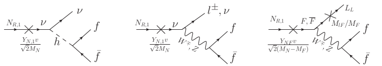
Figure 1: Feynman diagrams of DM decay in Model 1. The first two are the dominant processes to drive the decay of the DM $N_{R,1}$, the last decay channel goes via virtual vector-like fermion through the mixing $M_{lF}$.

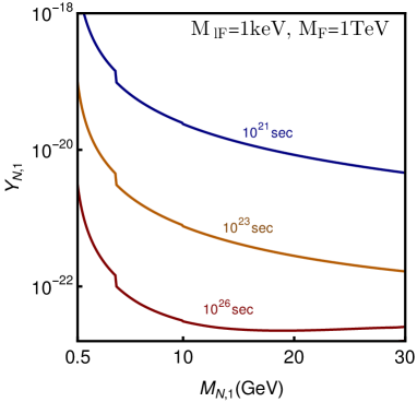
Figure 2: Contours of DM($N_{R,1}$) lifetime in the $M_{N,1}-Y_{N_{1}}$-plane.

Indirect detection constraints put a lower bound of $\mathcal{O}(10^{26}\,{\rm sec})$ on the lifetime of a decaying DM Essig:2013goa . In fig. 2 we depict the lifetime contours of the DM as a function of DM mass and coupling. Evidently, in order to satisfy this constraint one needs very small Yukawa coupling $Y_{N_{1}}$ as well as a very small mixing $M_{lF}\lesssim 1\,{\rm keV}$ to ensure a suppressed decay rate.

This value of $M_{lF}$ is much smaller than the mass of the heavy fermions and to check its stability we computed explicitly the one loop radiative contribution to $M_{lF}$. The corrections are as follows:

$$\Delta\,M_{F^{0}\nu}\sim\left\{\begin{aligned} &g^{2}_{2}\times\,\mathcal{F}(p^{2},m_{S,V},m_{f})\times M_{lF}~{}~{}\text{(F-V mediated loop)}\\ &g^{2}_{2}\times\,\mathcal{F}(p^{2},m_{S,V},m_{f})\times\frac{Y_{N}Y_{NF}\,v^{2}}{M_{N}-M_{F}}~{}~{}\text{($N_{i}$-V mediated loop)}\\ &Y_{N}\,Y_{NF}\,M_{N}\,\times\,\mathcal{F}(p^{2},m_{S,V},m_{f})~{}~{}\text{(H-$N_{i}$ loop)}.\end{aligned}\right.$$ (20)

and

$$\Delta\,M_{F^{\mp}l^{\pm}}\sim\left\{\begin{aligned} &g^{2}_{2}\times\mathcal{F}(p^{2},m_{S,V},m_{f})\times M_{lF}~{}~{}\text{(F-V loop)}\\ &g^{2}_{2}\times\mathcal{F}(p^{2},m_{S,V},m_{f})\times\frac{Y_{N}Y_{NF}\,v^{2}}{M_{N}-M_{F}}~{}~{}\text{(N${}_{i}$-V loop)}\\ &Y_{l}M_{lF}\times\mathcal{F}(p^{2},m_{S,V},m_{f})~{}~{}\text{(H-F loop).}\end{aligned}\right.$$ (21)

Here $\mathcal{F}(p^{2},m_{S,V},m_{f})=-\dfrac{1}{16\pi^{2}}\overset{1}{\underset{0}{\int}}dx\log\Delta(x)$ and $\Delta(x)=xm^{2}_{S,V}+(1-x)m^{2}_{f}-x(1-x)p^{2}$ with $m_{S,V,f}$ being the mass of the scalar, gauge boson or fermion in the loop and $p$ denotes the incoming momentum. The parentheses in each case denote the particles running in the corresponding loops where $F=F^{0},F^{-}$, $V=W^{\pm},Z,\gamma$ and $H$ denotes the SM higgs doublet.

So, if $Y_{NF}\,\leq\,10^{-10}$ then the corrections are too small to change substantially the mixing and affect the phenomenology. The coupling $Y_{N_{1}F}$ has to be $\mathcal{O}(10^{-12})$ for freeze-in mechanism and it is natural to assume all $Y_{N_{i}F}$ couplings are of same order, producing negligible radiative corrections.

The neutrino masses can be explained via type-I seesaw mechanism with appropriate values of $Y_{N,2,3}$ and $M_{N,2,3}$, leaving one vanishing mass eigenstate. For RH neutrino masses $M_{N,2,3}$ around $10-100$ GeV also those Yukawas are small, below $10^{-7}$, but substantially larger than all the others. So for the neutrino sector, the model is similar to the $\nu$SM model Asaka:2005pn ; Shaposhnikov:2006xi ; Shaposhnikov:2006nn , and indeed it may be possible to produce here also the baryon asymmetry of the Universe through the oscillations of the $N_{2,3}$ states. On the other hand in this case the production of the lightest heavy neutrino $N_{1}$ goes via another production mechanism than the Fuller-Shi mechanism Shi:1998km and does not have to rely on the presence of a very large lepton asymmetry.

Some positive and negative aspects of this simple-minded scenario are:

• It is simple and minimalistic, and postulates no additional charge, discrete or continuous, for the DM particle.

• The scenario is technically natural. It is shown by explicit calculation that not only the Yukawas but also the additional, bare mass terms involving $F$ are stable against radiative corrections for certain regions in the parameter space.

• However, justifying the ultra-small Yukawa interactions $\sim 10^{-20}$, and explaining why they are not zero to start with, is a potential difficulty. Also it appears that there are three different Yukawa coupling sizes, related to the neutrino masses, the freeze-in mechanism and the DM decay, which have to be chosen ad-hoc.

• $M_{lF}$ are ‘technically natural’ but being vectorlike bare mass terms one would naturally expect them to be in the same ballpark as $M_{F}$. But constraints on DM decay forces $M_{lF}\leq 1\,{\rm keV}\,\ll M_{F}$ which is difficult to explain.

2.2 Model 2

In the second model we have the same fermions as in the previous one, but we have added a new $U(1)_{DM}$ gauge group and one charged scalar field ($\Phi$) which breaks the $U(1)_{DM}$ symmetry. The particle content and their charges under the $SM\otimes U(1)$ gauge groups are presented in tab. 2.

Fields	$SU(3)_{c}$	$SU(2)_{L}$	$U(1)_{Y}$	$U(1)_{DM}$
$L_{L}$	1	2	-1/2	0
$l_{R}$	1	1	-1	0
$H$	1	2	1/2	0
$N_{R,2,3}$	1	1	0	0
$\psi\equiv N_{R,1}$	1	1	0	3
$F=\left(\begin{matrix}F^{0}\\ F^{-}\end{matrix}\right)$	1	2	-1/2	2
$\overline{F}=\left(\begin{matrix}\overline{F}^{0}\\ F^{+}\end{matrix}\right)$	1	$\overline{2}$	1/2	- 2
$\Phi$	1	1	0	1

Table 2: The quantum numbers of Lepton, Higgs of SM and newly added fields under the SM as well as $U(1)_{DM}$ gauge groups.

The SM Lagrangian has to be extended with the following terms due to the addition of the new fields and extra $U(1)_{DM}$ gauge group.

• The renormalizable terms :

  $$\mathcal{L}_{4}\, = \,\overline{F}i\mathchoice{\ooalign{$\hfil\displaystyle\mkern 0.0mu/\hfil$\crcr$\displaystyle D$}}{\ooalign{$\hfil\textstyle\mkern 0.0mu/\hfil$\crcr$\textstyle D$}}{\ooalign{$\hfil\scriptstyle\mkern 0.0mu/\hfil$\crcr$\scriptstyle D$}}{\ooalign{$\hfil\scriptscriptstyle\mkern 0.0mu/\hfil$\crcr$\scriptscriptstyle D$}}^{F}\,F+\overline{\psi}i\mathchoice{\ooalign{$\hfil\displaystyle\mkern 0.0mu/\hfil$\crcr$\displaystyle D$}}{\ooalign{$\hfil\textstyle\mkern 0.0mu/\hfil$\crcr$\textstyle D$}}{\ooalign{$\hfil\scriptstyle\mkern 0.0mu/\hfil$\crcr$\scriptstyle D$}}{\ooalign{$\hfil\scriptscriptstyle\mkern 0.0mu/\hfil$\crcr$\scriptscriptstyle D$}}^{\psi}\,\psi-M_{F}\overline{F}F-M_{\psi}\overline{\psi}\psi+\overline{N}_{R,i}i\mathchoice{\ooalign{$\hfil\displaystyle\mkern 0.0mu/\hfil$\crcr$\displaystyle\partial$}}{\ooalign{$\hfil\textstyle\mkern 0.0mu/\hfil$\crcr$\textstyle\partial$}}{\ooalign{$\hfil\scriptstyle\mkern 0.0mu/\hfil$\crcr$\scriptstyle\partial$}}{\ooalign{$\hfil\scriptscriptstyle\mkern 0.0mu/\hfil$\crcr$\scriptscriptstyle\partial$}}\,N_{R,i}-\frac{M_{N,i}}{2}\overline{N}^{c}_{R,i}N_{R,i}$$ (47)

  $$-Y_{\nu,i}\overline{N}_{R,i}L_{L}H+\left(D^{\Phi}_{\mu}\Phi\right)^{\dagger}(D^{\mu\,\Phi}\Phi)-\frac{m^{2}_{\Phi}}{2}\Phi^{\dagger}\Phi-\lambda_{H\Phi}\Phi^{\dagger}\Phi\,H^{\dagger}H-\lambda_{\Phi}(\Phi^{\dagger}\Phi)^{2}$$

  $$-\frac{1}{4}B^{D}_{\mu\nu}B^{D\,\mu\nu}.$$

  where $D^{F}_{\mu}=\partial_{\mu}-ig_{w}\dfrac{\tau^{a}}{2}W^{a}_{\mu}-\dfrac{1}{2}ig_{Y}B_{Y\mu}-2ig_{D}Z_{D\mu}$,$\,D^{\psi}_{\mu}\,=\,\partial_{\mu}-3ig_{D}Z_{D\mu}$, $D^{\Phi}_{\mu}\,=\,\partial_{\mu}-ig_{D}Z_{D\mu}$ and $B^{D}_{\mu\nu}\,=\,\partial_{\mu}Z_{D\nu}-\partial_{\nu}Z_{D\mu}$.

• The dimension-5 terms :

  $$\mathcal{L}_{5}\,=\, - \frac{1}{M_{Pl}}\bigg{[}\overline{N}^{c}_{R,i}N_{R,i}\left(\Phi^{\dagger}\Phi+H^{\dagger}H\right)+\overline{F}F\left(\Phi^{\dagger}\Phi+H^{\dagger}H\right)+\overline{\psi}\psi\left(\Phi^{\dagger}\Phi+H^{\dagger}H\right)$$ (48)

  $$+(\overline{L}^{c}_{L}H)(L_{L}H)+(\overline{F}\sigma^{\mu\nu}F+\overline{\psi}\sigma^{\mu\nu}\psi)B^{Y}_{\mu\nu}\bigg{]}$$

  $$- \frac{f_{1}}{M_{Pl}}\left(\overline{F}H\,\psi\Phi^{\dagger}+h.c\right)-\frac{f_{2}}{M_{Pl}}\left(\overline{F}_{R}L_{L}\Phi^{2}+h.c\right).$$

  The Wilson coefficients $f_{1}$ and $f_{2}$ can be $\ll 1$ if the corresponding dimension-5 terms are generated via some loop-induced diagrams at the Planck scale.

After the field $\Phi$ acquires a vacuum expectation value ($v_{D}$) the $U(1)_{DM}$ symmetry is spontaneously broken and the corresponding gauge boson called dark gauge-boson ($Z_{D}$) gets a mass $M_{Z_{D}}\,\sim\,g_{D}v_{D}$ and one can expand the Lagrangian with the replacement $\Phi\,=(v_{D}+S)/\sqrt{2}$ in the unitary gauge. Similarly one can replace $H\rightarrow\,(v+h)/\sqrt{2}$ in order to obtain possible mass terms and Higgs interaction terms. The lepton flavour violating decay $\mu\rightarrow e\gamma$ is mediated by $F^{0}-W^{-}$ loop or $F^{-}-Z$ loop and the rate is dictated by the $L_{L}-F$ mixing angle $\theta_{-}\sim f_{2}v^{2}_{D}/M_{F}M_{Pl}$. The present limit on the branching ratio of $\mu\rightarrow e\gamma$ TheMEG:2016wtm puts a upper limit on $v_{D}$. On the other hand, the out-of-equillibrium condition on $\psi$ puts a lower bound on $v_{D}$ since the $Z_{D}$-boson can thermalize the DM state via $2\rightarrow 2$ scatterings. We found $v_{D}=7\times 10^{7}\,{\rm GeV}$ to be consistent with both $\mu\rightarrow e\gamma$ as well as DM production.

The phenomenology of this model keeping $v_{D}=7\times 10^{7}\,{\rm GeV}$ fixed, can briefly be stated as:

• DM Production : The dominant contribution to the $\psi$ relic density originates also here from the decay $F\rightarrow\,\psi\,H$. But in this case, the interaction is generated by the dimension-5 effective operator $\dfrac{f_{1}v_{D}}{M_{Pl}}\bar{F}H\,\psi$. In the right panel of fig. 3 we have shown the DM relic density as a function of $f_{1}$ and DM mass, where we fix the mass of $F$ to be 1 TeV. The observed relic density can be achieved for $f_{1}\approx\,1$ and $v_{D}\,=7\,\times\,10^{7}\,$GeV.

  

  

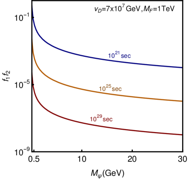
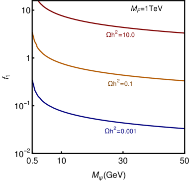
  Figure 3: Left panel: DM lifetime contours in the $f_{1}f_{2}$ vs. $M_{\psi}$ plane. Right panel: relic density contours in the $f_{1}-M_{\psi}$ plane. In both the cases we have considered $v_{D}=7\times 10^{7}\,{\rm GeV}$ and $M_{F}=1\,{\rm TeV}$.

• DM decay : The decay of DM $\psi$ into SM final states are taking place via intermediate off-shell fermions and are therefore driven by the factor $f_{1}f_{2}\,v\,v^{3}_{D}/(M^{2}_{Pl}\,M_{\psi}M_{F})$ with a combination of dimension 5 vertices. In the left panel of fig. 3 we have shown the DM lifetime contours in the plane of DM mass $M_{\psi}$ and Wilson coefficients $f_{1}f_{2}$. For a chosen benchmark with $v_{D}\,=7\,\times\,10^{7}\,$GeV we found that the product of the two Wilson coefficients $f_{1}f_{2}$ has to be smaller than $\sim\,10^{-5}$ to achieve a dark matter lifetime of $10^{26}$ sec or more (see fig. 3, left-panel). So in this case the suppressed decay can be achieved also for moderately small couplings. Note that the $f_{1}$ coupling also drives the DM production and has to remain of order ${\cal O}(1)$ for DM masses in the tens of GeV, in order to produce a sufficient DM abundance, as shown in fig. 3(right-panel).

  

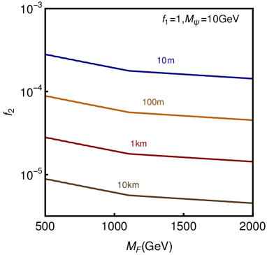
  Figure 4: $F^{0}$ decay length contours in the $f_{2}-M_{F}$ plane. Here we have assumed $v_{D}=7\times 10^{7}\,{\rm GeV}$ and $M_{\psi}=10\,{\rm GeV}$. We have also chosen $f_{1}=1$ in order to have the freeze-in relic density in the correct ballpark.

• $F^{0}$ production and decay at colliders: The electroweak states $F^{\pm},F^{0},\overline{F}^{0}$ can be produced at colliders via Drell-Yan production. Generically, we expect the charged states to be slightly heavier than the neutral ones and be able to decay promptly into the neutral states and pions Cirelli:2005uq . So a substantial population of $F^{0},\overline{F}^{0}$ particles can arise even at the LHC, if their mass is below $1$ TeV. The decay of $F^{0}$ occurs both in pure SM modes ($W(Z)l(\nu)$) or in a mixed SM-BSM mode ($\psi\,h$). The latter mode contributes to freeze-in relic density of $\psi$ and hence has to be very slow while the decay into SM states can occur faster via the mixing $f_{2}v^{2}_{D}/M_{Pl}M_{F}$. The dominant part of the decay width of $F^{0}$ is therefore given by,

  $$\Gamma_{F^{0}\rightarrow\,W(Z)l(\nu)}\,=\,\frac{g^{2}_{weak}|V_{\nu\,F}|^{2}(c^{2}_{V}+c^{2}_{A})}{8\pi}\frac{M^{3}_{F}}{M^{2}_{V}}\left(1-\frac{M^{2}_{V}}{M^{2}_{F}}\right)^{2}\left(1+\frac{2\,M^{2}_{V}}{M^{2}_{F}}\right).$$ (49)

  where $V_{\nu F}$ is proportional to $f_{2}v^{2}_{D}/M_{Pl}M_{F}$. Depending on the value of $f_{2}$, $F^{0}$ can have a decay length of few meters to one kilometer as shown in fig. 4. So the mother particle in this scenario can realised both displaced vertices or missing energy signatures and can be searched at present and future colliders Arcadi:2014tsa ; Acharya:2014nyr ; Curtin:2018mvb .

  Of course we could also lower the scale of the non-renormalizable operators from $M_{Pl}$ to some intermediate scale $\Lambda$ and obtain still a consistent picture, as long as we satisfy $\dfrac{f_{1}v_{D}}{\Lambda}\sim 10^{-12}$ and the DM lifetime remains sufficiently long. Note that while the production is driven by the factor $\dfrac{v_{D}}{\Lambda}$, the decay depends on the combination $\dfrac{f_{1}f_{2}vv_{D}^{3}}{\Lambda^{2}M_{\psi}M_{F}}\leq 10^{-24}\dfrac{f_{2}vv_{D}}{f_{1}M_{\psi}M_{F}}$ assuming the value of the effective coupling from the FIMP production. Then for a dark matter mass of $10$ GeV, this gives a lower bound on the value of $v_{D}$ as

  $$v_{D}\leq 62\;\frac{f_{1}}{f_{2}}\;M_{F}$$ (50)

  We see therefore that in that case the dark Sector could be characterised by a similar mass scale for the scalar and fermionic states and the UV completion of the model may appear way below the Planck scale.

The overall advantages of this framework are:

• The effective operators in eq. (48), suppressed by the Planck mass, successfully generate the effective couplings involved in DM decay as well as freeze-in in the right ballpark, without the need to fine-tune the Wilson coefficients. Thus a rather tantalizing connection with UV completion at the Planck scale arises, even if also lower values of the cut-off scale are possible.

• The scenario is cosmologically consistent and anomaly free.

• The generation of neutrino masses and as well as various constraints from electroweak phenomenology are not affected.

• The addition of the $U(1)_{D}$ breaking scalar $\Phi$ with the mass scale it brings in, enables one to achieve vacuum stability all the way to Planck scale EliasMiro:2012ay .

On the other hand, there is no direct connection between neutrino phenomenology and DM phenomenology. It is straight-forward to understand that such a connection can readily be established if we elevate the $U(1)_{\rm DM}$ to $U(1)_{L_{\mu}-L_{\tau}}$ Baek:2008nz ; Baek:2015fea ; Patra:2016shz ; Altmannshofer:2016jzy ; Biswas:2016yjr ; Biswas:2016yan ; Biswas:2017ait or $U(1)_{B-L}$ Okada:2010wd ; Lindner:2011it ; Okada:2012sg ; Basso:2012ti ; Basak:2013cga ; Sanchez-Vega:2014rka ; Guo:2015lxa ; Rodejohann:2015lca ; Patra:2016ofq ; Biswas:2017tce ; Okada:2018ktp ; Bhattacharya:2019tqq . We consider $U(1)_{L_{\mu}-L_{\tau}}$ in the next model.

3 Gauged $U(1)_{L_{\mu}-L_{\tau}}$ Model

Now we will move to the gauged $U(1)_{L_{\mu}-L_{\tau}}$ model. This model can explain neutrino mass and give a decaying FIMP dark matter without any ad-hoc symmetry barring the $U(1)_{L_{\mu}-L_{\tau}}$. As has been mentioned in the introduction, such a scenario can help in identifying a common UV completion of the modeling of slowly decaying DM and the observed pattern in the neutrino sector, the degree of oscillation required to explain the data on atmospheric neutrinos. In addition to the SM particle content we consider again a symmetry breaking scalar $\Phi$ and a vector-like fermion $\psi$, playing the role of the DM. So in this case the dark matter particle is not one of the heavy neutrinos, but it is still tightly related to the leptonic sector via the gauge symmetry and the gauge symmetry preserving interactions.

The particle content of our model and their charges under all the gauge groups are shown in tab. 3.

Fields	Spin	$SU(3)_{c}$	$SU(2)_{L}$	$U(1)_{Y}$	$U(1)_{L_{\mu}-L_{\tau}}$
$L_{L\,e}$	1/2	1	2	-1/2	0
$l_{R\,e}$	1/2	1	1	-1	0
$N_{R\,e}$	1/2	1	1	0	0
$L_{L\,\mu}$	1/2	1	2	-1/2	1
$l_{R\,\mu}$	1/2	1	1	-1	1
$N_{R\,\mu}$	1/2	1	1	0	1
$L_{L\,\tau}$	1/2	1	2	-1/2	-1
$l_{R\,\tau}$	1/2	1	1	-1	-1
$N_{R\,\tau}$	1/2	1	1	0	-1
$\Phi$	0	1	1	0	1
$\psi_{L,R}$	1/2	1	1	0	4

Table 3: The quantum numbers of the SM Leptons and added BSM fields under SM as well as $U(1)_{L_{\mu}-L_{\tau}}$ gauge group.

Apart from the tree level terms we have also considered possible higher order operators and the Lagrangian of the model consist of three pieces:

$$\mathcal{L}=\mathcal{L}_{dim-4}+\mathcal{L}_{dim-5}+\mathcal{L}_{dim-6}.$$ (51)

The dim-4 terms are given by,

$$\mathcal{L}_{dim-4} \supset \overline{N}_{Ri}i\mathchoice{\ooalign{$\hfil\displaystyle\mkern 0.0mu/\hfil$\crcr$\displaystyle D$}}{\ooalign{$\hfil\textstyle\mkern 0.0mu/\hfil$\crcr$\textstyle D$}}{\ooalign{$\hfil\scriptstyle\mkern 0.0mu/\hfil$\crcr$\scriptstyle D$}}{\ooalign{$\hfil\scriptscriptstyle\mkern 0.0mu/\hfil$\crcr$\scriptscriptstyle D$}}^{N,i}N_{Ri}-\frac{1}{2}M_{ee}\overline{N}^{c}_{Re}N_{Re}-\frac{1}{2}M_{\mu\tau}\left(\overline{N}^{c}_{R\mu}N_{R\tau}+\overline{N}^{c}_{R\tau}N_{R\mu}\right)$$ (70)

$$-\frac{1}{2}h_{e\mu}\left(\overline{N}^{c}_{Re}N_{R\mu}+\overline{N}^{c}_{R\mu}N_{Re}\right)\Phi^{\dagger}-\frac{1}{2}h_{e\tau}\left(\overline{N}^{c}_{Re}N_{R\tau}+\overline{N}^{c}_{R\tau}N_{Re}\right)\Phi$$

$$+\overline{\psi}i\mathchoice{\ooalign{$\hfil\displaystyle\mkern 0.0mu/\hfil$\crcr$\displaystyle D$}}{\ooalign{$\hfil\textstyle\mkern 0.0mu/\hfil$\crcr$\textstyle D$}}{\ooalign{$\hfil\scriptstyle\mkern 0.0mu/\hfil$\crcr$\scriptstyle D$}}{\ooalign{$\hfil\scriptscriptstyle\mkern 0.0mu/\hfil$\crcr$\scriptscriptstyle D$}}^{\psi}\psi-M_{\psi}\overline{\psi}{\psi}-\underset{\alpha=e,\mu,\tau}{\sum}Y_{\alpha}\overline{L}_{L\alpha}N_{R\alpha}H+V(\Phi,H)$$

$$-\dfrac{1}{4}B^{D}_{\mu\nu}B^{D\mu\nu}-\dfrac{\sin\epsilon}{2}B^{Y}_{\mu\nu}B^{D\mu\nu},$$

with the scalar potential,

$$V(\Phi,H)=-m^{2}_{\Phi}\Phi^{\dagger}\Phi+\lambda_{\Phi}(\Phi^{\dagger}\Phi)^{2}+\lambda_{H\,\Phi}\;\Phi^{\dagger}\Phi\;H^{\dagger}H.$$ (71)

The presence of the term $\lambda_{H\Phi}\Phi^{\dagger}\Phi H^{\dagger}H$ causes mixing between the scalars $h$ and $\phi$ when the respective scalar fields acquire v.e.vs $v$ and $v_{D}$ respectively. We have minimized the potential $V(\Phi,H)$ to obtain,

$$v\,=\,\left(\frac{2m^{2}_{H}\lambda_{\Phi}-\lambda_{H\Phi}m^{2}_{\Phi}}{\lambda^{2}_{H\Phi}-4\lambda_{H}\lambda_{\Phi}}\right)^{1/2}\hskip 14.22636pt{\rm and}\hskip 14.22636ptv_{D}\,=\,\left(\frac{2m^{2}_{\Phi}\lambda_{H}-\lambda_{H\Phi}m^{2}_{H}}{\lambda^{2}_{H\Phi}-4\lambda_{H}\lambda_{\Phi}}\right)^{1/2}.$$ (72)

Diagonalizing the mass matrix give rise to the mass eigenstates:

$$\begin{pmatrix}h_{1}\\ h_{2}\end{pmatrix}=\begin{pmatrix}\cos\theta_{h}&\sin\theta_{h}\\ -\sin\theta_{h}&\cos\theta_{h}\end{pmatrix}\begin{pmatrix}h\\ \phi\end{pmatrix}$$ (73)

where the mixing angle $\theta_{h}\approx\dfrac{\lambda_{H\Phi}vv_{D}}{(m^{2}_{\Phi}-m^{2}_{h})+\frac{v^{2}}{2}(\lambda_{H\Phi}-\lambda_{H})+\frac{v^{2}_{D}}{2}(\lambda_{\Phi}-\lambda_{H\Phi})}$.

The kinetic mixing term $\dfrac{\sin\epsilon}{2}B^{Y}_{\mu\nu}B^{D\mu\nu}$ in the Lagrangian $\mathcal{L}_{dim-4}$ will induce a mixing between the SM-$Z$ boson and $L_{\mu}-L_{\tau}$ gauge boson $Z_{D}$. The mixing angle is given by Arcadi:2018tly ,

$$\tan\,2\alpha=-\frac{\hat{m}^{2}_{Z}\sin\theta_{W}\sin\,2\epsilon}{\hat{M}^{2}_{Z_{D}}-\hat{m}^{2}_{Z}(\cos^{2}\epsilon-\sin^{2}\epsilon\sin^{2}\theta_{W})}\;,$$ (74)

where $\hat{m}_{Z}$, $\hat{M}_{Z_{D}}$ are the bare masses for the SM-Z boson and $Z_{D}$ boson respectively. Clearly the mixing angle $\alpha$ is strongly suppressed if the dark gauge boson $Z_{D}$ is much heavier than the $Z$.

This mixing in turn induces a $\bar{\psi}\psi\,Z$ coupling $g_{\bar{\psi}\psi\,Z}=\dfrac{\sin\alpha}{\cos\epsilon}g_{D}$ and modifies the lepton couplings to SM $Z$ boson:

$$g_{f_{L}\,Z} = \frac{e}{\sin\theta_{W}\,\cos\theta_{W}}\cos\alpha\left[T_{3}\left(1+\sin\theta_{W}\,\tan\epsilon\tan\alpha\right)-Q_{f}\left(\sin^{2}\theta_{W}+\sin\theta_{W}\tan\epsilon\tan\alpha\right)\right]$$ (75)

$$\pm\,g_{D}\frac{\sin\alpha}{\cos\epsilon}$$

$$g_{f_{R}\,Z} = -\frac{e}{\sin\theta_{W}\,\cos\theta_{W}}\cos\alpha\,Q_{f}\left(\sin^{2}\theta_{W}+\sin\theta_{W}\tan\epsilon\tan\alpha\right)\pm\,g_{D}\frac{\sin\alpha}{\cos\epsilon},$$ (76)

where $\left(+g_{D}\frac{\sin\alpha}{\cos\epsilon}\right)$ is relevant for $f=\mu$ and $\left(-g_{D}\frac{\sin\alpha}{\cos\epsilon}\right)$ is for $f=\tau$. The first term in each case is the corresponding coupling for other SM fermions.

For our choice of parameters $g_{D}=0.01,v_{D}\geq 10^{7}\,{\rm GeV}$ we get $\hat{M}_{Z_{D}}\geq 10^{5}\,{\rm GeV}$ and hence $\sin\alpha\leq 10^{-7}$ even for $\sin\epsilon\approx 1$. This happens because the mixing angle $\alpha$ is proportional to $\hat{m}^{2}_{Z}/\hat{M}^{2}_{Z_{D}}$ which is always small due to large $v_{D}$. This causes a $\bar{\psi}\psi\,Z$ coupling $\leq\mathcal{O}(10^{-8})$ and thus one can neglect the effect of kinetic mixing in the following analysis.

The dimension-5 Lagrangian consists of the following terms,

$$\mathcal{L}_{dim-5} \supset \frac{f_{1}}{\Lambda}\overline{\psi}\psi\left(\Phi^{\dagger}\Phi+H^{\dagger}H\right)+\frac{f_{2}}{\Lambda}\;\overline{N}^{c}_{Re}N_{Re}\Phi^{\dagger}\Phi$$ (77)

$$+\frac{f_{3}}{\Lambda}\left(\overline{N}^{c}_{R\mu}N_{R\mu}\Phi^{\dagger 2}+h.c\right)+\frac{f_{3^{\prime}}}{\Lambda}\left(\overline{N}^{c}_{R\tau}N_{R\tau}\Phi^{2}+h.c\right)+\frac{f_{5}}{\Lambda}\underset{\alpha=e,\mu,\tau}{\sum}\overline{L}^{c}_{L\alpha}H\overline{L}_{L\alpha}H$$

$$+\frac{f_{6}}{\Lambda}H\left(\overline{L}_{Le}N_{R\mu}\Phi^{\dagger}+\overline{L}_{L\mu}N_{Re}\Phi\right)+\frac{f_{7}}{\Lambda}H\left(\overline{L}_{Le}N_{R\tau}\Phi+\overline{L}_{L\tau}N_{Re}\Phi^{\dagger}\right)$$

There is no interaction between DM $\psi$ and other fields due to $L_{\mu}-L_{\tau}$ charge of the DM at this level but these terms have an important role to play in the neutral lepton mass matrix and thus in the $\psi-N$ mixing. The dimension-6 terms $\mathcal{L}_{dim-6}$ induce the lowest order mixing between DM $\psi$ and SM sector:

$$\mathcal{L}_{dim-6} \supset \frac{f_{4}}{\Lambda^{2}}\left[\left(\overline{\psi}_{L}N_{R\mu}+\overline{\psi}_{R}N^{c}_{R\tau}\right)\Phi^{3}+h.c\right]+\frac{f_{8}}{\Lambda^{2}}H\left(\overline{L}_{L\mu}N_{R\tau}\Phi^{\dagger 2}+\overline{L}_{L\tau}N_{R\mu}\Phi^{2}\right).$$

Note that here we consider a generic cut-off scale $\Lambda\leq M_{Pl}$ and contrary to the previous case, we consider as well the dimension 6 operators, as there is no mixing between the neutrinos and the dark matter from the lower order operators.

3.1 Neutrino Phenomenology

The neutral lepton mass terms after $U(1)_{L_{\mu}-L_{\tau}}$ breaking takes the form $V^{\dagger}\mathcal{M}_{0}V$, where $V=(\nu^{c}_{L,\alpha},N_{R,\alpha},\Psi_{R})^{T}$ with $\alpha=e,\mu,\tau$ and $\Psi_{R}=(\psi^{c}_{L},\psi_{R})$. The mass matrix is,

$$\mathcal{M}_{0}=\left(\begin{matrix}0&\dfrac{Y_{\alpha}v}{\sqrt{2}}&0\\ \vspace{1mm}\dfrac{Y^{T}_{\alpha}v}{\sqrt{2}}&\mathcal{M}_{N}&\dfrac{Y_{N\psi}v^{3}_{D}}{\Lambda^{2}}\\ \vspace{1mm}0&\dfrac{Y^{T}_{N\psi}v^{3}_{D}}{\Lambda^{2}}&\mathcal{M}_{\Psi}\end{matrix}\right).$$ (79)

where,

$$Y_{\alpha}\, = \,\left(\begin{matrix}Y_{e}&\dfrac{f_{6}v_{D}}{\Lambda}&\dfrac{f_{7}v_{D}}{\Lambda}\\ \vspace{2mm}\dfrac{f_{6}v_{D}}{\Lambda}&Y_{\mu}&\dfrac{f_{8}v^{2}_{D}}{\Lambda^{2}}\\ \vspace{2mm}\dfrac{f_{7}v_{D}}{\Lambda}&\dfrac{f_{8}v^{2}_{D}}{\Lambda^{2}}&Y_{\tau}\end{matrix}\right),\hskip 28.45274ptY_{N\psi}\,=\,\left(\begin{matrix}0&0\\ \vspace{1mm}f_{4}&0\\ \vspace{1mm}0&f_{4}\end{matrix}\right),$$ (80)

$$\mathcal{M}_{N}\, = \,\left(\begin{matrix}\frac{1}{2}M_{ee}&h_{e\mu}v_{D}&h_{e\tau}v_{D}\\ \vspace{1mm}h^{T}_{e\mu}v_{D}&\dfrac{f_{3}v^{2}_{D}}{\Lambda}&M_{\mu\tau}\\ \vspace{1mm}h^{T}_{e\tau}v_{D}&M_{\mu\tau}&\dfrac{f_{3}v^{2}_{D}}{\Lambda}\end{matrix}\right),\hskip 28.45274pt\mathcal{M}_{\Psi}\,=\,\left(\begin{matrix}0&M_{\psi}\\ \vspace{1mm}M_{\psi}&0\end{matrix}\right).$$ (81)

For simplicity we neglect $f_{8}v^{2}_{D}/\Lambda^{2}$ since this term is suppressed by $v_{D}/\Lambda$ compared to the terms proportional to $f_{6,7}$, as well as the terms ${\cal O}(v_{D}^{3}/\Lambda^{2})$ in $\mathcal{M}_{0}$. Diagonalizing the mass matrix $\mathcal{M}_{0}$ we obtain then,

$$\mathcal{M}_{N} = \left(\frac{Y_{\alpha}v}{\sqrt{2}}\right)U_{PMNS}\left(m^{diag}_{\nu}\right)^{-1}U^{T}_{PMNS}\left(\frac{Y_{\alpha}v}{\sqrt{2}}\right)^{T}.$$ (82)

Here $m^{diag}_{\nu}=\textrm{diag}(m_{1},m_{2},m_{3})$, where $m_{1}$ is mass of the lightest neutrino. Comparing the (22) and (33) elements of the above equation with $\mathcal{M}_{N}$ in eq. (81) we get,

$$\left(\frac{f_{6}v_{D}}{\Lambda}\right)^{2}\left(\frac{U^{2}_{e1}}{m_{1}}+\frac{U^{2}_{e2}}{m_{2}}+\frac{U^{2}_{e3}}{m_{3}}\right)+2\left(\frac{f_{6}v_{D}}{\Lambda}Y_{\mu}\right)\left(\frac{U_{e1}U_{\mu 1}}{m_{1}}+\frac{U_{e2}U_{\mu 2}}{m_{2}}+\frac{U_{e3}U_{\mu 3}}{m_{3}}\right)$$

$$\hskip 176.407pt+Y^{2}_{\mu}\left(\frac{U^{2}_{\mu 1}}{m_{1}}+\frac{U^{2}_{\mu 2}}{m_{2}}+\frac{U^{2}_{\mu 3}}{m_{3}}\right)=\frac{2}{v^{2}}\frac{f_{3}v^{2}_{D}}{\Lambda}$$ (83)

and,

$$\left(\frac{f_{7}v_{D}}{\Lambda}\right)^{2}\left(\frac{U^{2}_{e1}}{m_{1}}+\frac{U^{2}_{e2}}{m_{2}}+\frac{U^{2}_{e3}}{m_{3}}\right)+2\left(\frac{f_{7}v_{D}}{\Lambda}Y_{\tau}\right)\left(\frac{U_{e1}U_{\tau 1}}{m_{1}}+\frac{U_{e2}U_{\tau 3}}{m_{2}}+\frac{U_{e3}U_{\tau 3}}{m_{3}}\right)$$

$$\hskip 176.407pt+Y^{2}_{\tau}\left(\frac{U^{2}_{\tau 1}}{m_{1}}+\frac{U^{2}_{\tau 2}}{m_{2}}+\frac{U^{2}_{\tau 3}}{m_{3}}\right)=\frac{2}{v^{2}}\frac{f_{3^{\prime}}v^{2}_{D}}{\Lambda}.$$ (84)

Here $U_{\alpha i}$ are elements of the $U_{PMNS}$ matrix:

$$U_{PMNS} \equiv \left(\begin{matrix}c_{12}c_{13}&s_{12}c_{13}&s_{13}e^{-i\delta_{\rm CP}}\\ -s_{12}c_{23}-c_{12}s_{23}s_{13}e^{i\delta_{\rm CP}}&(c_{12}c_{23}-s_{12}s_{23}s_{13}e^{i\delta_{\rm CP}})&s_{23}c_{13}\\ s_{12}s_{23}-c_{12}c_{23}s_{13}e^{i\delta_{\rm CP}}&(-c_{12}s_{23}-s_{12}c_{23}s_{13}e^{i\delta_{\rm CP}})&c_{23}c_{13}\end{matrix}\right)\times\mathcal{P}$$

with $\mathcal{P}\,=\,{\rm diag}(1,e^{i\alpha/2},e^{i\beta/2})$ and $c_{12}=\cos\theta_{12}$ etc. The eqs. (83) and (84) essentially determine the parameter space of the model. Interestingly, in the usual $L_{\mu}-L_{\tau}$ scenario one does not consider the higher-dimensional terms and it becomes difficult to obtain a neutrino mass spectra consistent with the PLANCK constraint of $\underset{i=1,2,3}{\sum}|m_{\nu i}|\leq 0.11\,{\rm eV}$ Aghanim:2018eyx . In our case instead we obtain a large parameter space satisfying neutrino oscillation data which also satisfy the PLANCK constraint as we will discuss below.

By diagonalizing the mass matrix $\mathcal{M}_{0}$ one also obtains the mixing between DM $\psi$ and SM neutrinos which is given by,

$$U_{\nu\psi}\approx-\frac{Y^{T}_{N\Psi}Y^{T}_{\alpha}}{\mathcal{M}_{N}\mathcal{M}_{\Psi}}\left(\frac{vv^{3}_{D}}{\sqrt{2}\Lambda^{2}}\right).$$ (86)

Following eqs. (83), (84) and (86) one can understand that $v_{D}/\Lambda$ and $v_{D}^{2}/\Lambda$ are again the key parameters and they determine now both the neutrino as well as the DM phenomenology. One can further see from eq. (86) that the DM-SM neutrino mixing angle $U_{\nu\psi}$ is not only determined by the combination $v^{3}_{D}/\Lambda^{2}$ but also by the sterile neutrino-active neutrino mixing angle $U_{\nu N}\simeq Y^{T}_{\alpha}v/\sqrt{2}\mathcal{M}_{N}$ and thus the DM phenomenology is quite entangled with the neutrino phenomenology in this scenario.

Let us first consider the neutrino sector and eqs. (83) and (84). A large number of parameters appears there, and to understand the dependence on them one need to assume only some of them dominate in the equations. For example, if we consider the case $v_{D}/\Lambda\gg Y_{\mu,\tau}$ then only the first terms in eqs. (83) and (84) are important and under the assumption of $f_{6,7,3,3^{\prime}}\approx 1$, one needs $\Lambda\simeq\dfrac{v^{2}}{2}\left(\frac{U^{2}_{e1}}{m_{1}}+\frac{U^{2}_{e2}}{m_{2}}+\frac{U^{2}_{e3}}{m_{3}}\right)\sim 10^{14}\,{\rm GeV}$, similar to the scale needed by generating the light neutrino masses with the dimension-5 Weinberg operator. In the opposite extreme, taking $v_{D}/\Lambda\ll Y_{\mu,\tau}$, one obtains instead $Y^{2}_{i}\simeq\dfrac{2}{v^{2}}\dfrac{f_{3,3^{\prime}}v^{2}_{D}}{\Lambda}\left(\frac{U^{2}_{i1}}{m_{1}}+\frac{U^{2}_{i2}}{m_{2}}+\frac{U^{2}_{i3}}{m_{3}}\right)^{-1}\simeq 10^{-14}\,{\rm GeV}^{-1}\,\dfrac{f_{3,3^{\prime}}v^{2}_{D}}{\Lambda}$ (here $i=\mu,\tau$). Now it is clear that if $f_{3,3^{\prime}}v^{2}_{D}/\Lambda\lesssim 10^{-2}$ then the Majorana neutrino masses are of $\mathcal{O}(100{\rm MeV})$ and will have very suppressed mixing angles $\theta_{\nu N}\sim 10^{-5}$. These neutrinos will therefore be extremely long-lived and their late time decays will be in tension with BBN prediction of light-element abundances. A large value of $v^{2}_{D}/\Lambda$ will decrease the DM lifetime (following eq. (86)) and we will need to push $f_{4}$ to smaller values to make DM stable till today. Therefore only a window of values for $v^{2}_{D}/\Lambda$ is viable, where the lower bound is set by the neutrino sector and upper bound is dictated by the DM lifetime.

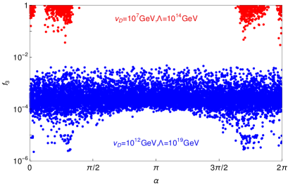
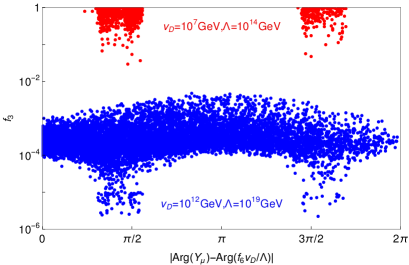
Figure 5: Left Panel: Value of the coupling $f_{3}$ giving a solution of the condition in eq. (83) as a function of the Majorana phase $\alpha$ in the PMNS mixing matrix. Right Panel: Value of the coupling $f_{3}$ giving a solution of the condition in eq. (83) as a function of the Yukawa and Wilson coefficients phases. For smaller values of $v_{D}$, a correlation among the phases becomes apparent, which disappears for larger values.

The intermediate situation $Y_{\mu,\tau}\simeq v_{D}/\Lambda$ is more interesting to look at, as then all the terms in the l.h.s are important. Under the assumption of $Y_{\mu,\tau}\simeq v_{D}/\Lambda$ with a scan over $v_{D}$ and $\Lambda$ we did not find any parameter point consistent with $|f_{3}|,|f_{3^{\prime}}|\leq 1$ for $v_{D}\lesssim 10^{7}\,{\rm GeV}$ and $\Lambda\lesssim 10^{14}\,{\rm GeV}$. This is mainly because keeping $Y_{\mu,\tau}\simeq v_{D}/\Lambda$ fixed if one reduces the values of $v_{D}$ and $\Lambda$, $v^{2}_{D}/\Lambda$ becomes too small and thus it is not possible to satisfy $|f_{3}|,|f_{3^{\prime}}|\leq 1$. We have chosen $v_{D}=10^{7}\,{\rm GeV}$, $\Lambda=10^{14}\,{\rm GeV}$ as our benchmark in the following analysis. For larger values of $v_{D},\Lambda$ with the same ratio $Y_{\mu,\tau}\simeq v_{D}/\Lambda$, the couplings $|f_{3}|,|f_{3^{\prime}}|$ can be very small and the eqs. (83) and (84) are satisfied without any cancellation among different terms in the l.h.s.. As an illustration we have shown in fig. 5 the allowed values of $\alpha$ and $|Arg(Y_{\mu})-Arg(f_{6}v_{D}/\Lambda)|$ for two different benchmarks $(v_{D},\Lambda)=(10^{7}\,{\rm GeV},10^{14}\,{\rm GeV})$ and $(10^{12}\,{\rm GeV},10^{19}\,{\rm GeV})$. Although the values of $v_{D}/\Lambda\simeq 10^{-7}$ in both the cases, $v^{2}_{D}/\Lambda$ is larger in the latter scenario. Thus the distribution of parameter points for $(v_{D},\Lambda)=(10^{7}\,{\rm GeV},10^{14}\,{\rm GeV})$(red-dotted) is shifted upward by a factor of $10^{5}$ compared to the case $(v_{D},\Lambda)=(10^{12}\,{\rm GeV},10^{19}\,{\rm GeV})$(blue-dotted). Thus we see that for $(v_{D},\Lambda)=(10^{7}\,{\rm GeV},10^{14}\,{\rm GeV})$ one needs cancellation among several terms in the l.h.s of eqs. (83) and (84). Such a cancellation occurs if $|Arg\left(Y_{\mu(\tau)}\right)-Arg\left(f_{6(7)}v_{D}/\Lambda\right)|\,\simeq\pi/2$ or $3\pi/2$ and $\alpha\simeq 0\,$or $\,2\pi$.

Fixed Parameters	Values	Varied Parameters	Ranges
$v_{D}$	$10^{7}$ GeV	$m_{1}$	$[0.001\,,0.026]\,{\rm eV}$
$\Lambda$	$10^{14}$ GeV	$\delta_{CP}$	$[0,2\pi]$
$|f_{6,7}|$	1	$\alpha$	$[0,2\pi]$
$|Y_{e,\mu,\tau}|$	$10^{-7}$	$\beta$	$[0,2\pi]$
$\theta_{12}$	33.85o	Arg($f_{6}$)	$[0,2\pi]$
$\theta_{23}$	48.35o	Arg($Y_{\mu}$)	$[0,2\pi]$
$\theta_{13}$	8.61o	Arg($f_{7}$)	$[0,2\pi]$
		Arg($Y_{\tau}$)	$[0,2\pi]$

Table 4: Parameters kept fixed during our analysis for producing fig. 6 and the parameters which have been varied within certain ranges are tabulated.

To explore the correlations in case of $v_{D}\sim 10^{7}\,{\rm GeV},\Lambda=10^{14}\,{\rm GeV}$, we keep some of the parameters appearing in eqs. (83) and (84) fixed while others are varied within specified ranges. A comprehensive list of all the parameters and their range is given in tab. 4. We have chosen the values of the varied parameters ($m_{1},\delta_{\rm CP},\alpha,\beta,Arg(Y_{\mu,\tau}),Arg(f_{6,7})$) randomly within specified ranges and points for which $|f_{3}|,|f_{3^{\prime}}|\leq 1$ are considered as viable points. We have presented results for normal hierarchy(NH) of neutrino masses. A correlation among several parameters can also be seen in fig. 6. The Majorana phase $\alpha$ tends to be either close to 0 or $2\pi$ while $\beta$ shows a peculiar pattern with $\delta_{\rm CP}$. We also found that small values of the lightest neutrino mass $m_{1}$ is disfavoured since that will enhance the left-hand side of eqs. (83) and (84) which in turn drives $|f_{3}|,|f_{3^{\prime}}|$ to be larger than unity thus violating perturbativity. We found a lower limit of $m_{1}\geq 0.0011$eV in our random scan over a billion points. Interestingly, $\delta_{\rm CP}$ is rather unconstrained in this scenario.

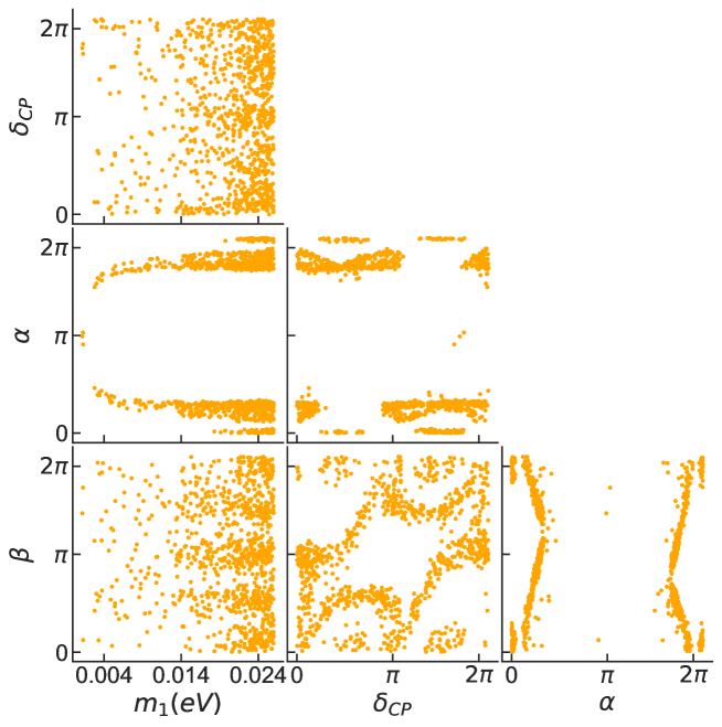
Figure 6: Correlation among different phases relevant for neutrino oscillation: the CP-phase($\delta_{\rm CP}$) and the Majorana phases ($\alpha,\beta$). The correlation of each of these phases with the lightest neutrino mass($m_{1}$) is shown in the left most column. These correlation is found under the assumption of tab. 4.

Since $m_{1}$ can not be arbitrarily low, we expect chances of observing neutrinoless double beta decay($0\nu\beta\beta$). The amplitude for $0\nu\beta\beta$ decay is given by,

$$\mathcal{A}^{0\nu\beta\beta}\propto\underset{i=e,\mu,\tau}{\sum}U^{2}_{ei}\;m_{i}\;\mathcal{M}_{\rm NME}(m_{i})+U^{2}_{\nu\psi}\;M_{\psi}\;\mathcal{M}_{\rm NME}(M_{\psi})$$ (87)

where $\mathcal{M}_{\rm NME}(\mu)$ is the nuclear matrix element (at the scale $\mu$). We have explicitly checked that the second term in eq. (87) (DM contribution) is negligible compared to the first term (active neutrino contribution) due to the smallness of the DM-SM neutrino mixing angle $U_{\nu\psi}$(see eq. (86)). In addition, for $M_{\psi}\gtrsim 100\,{\rm MeV}$ the nuclear matrix element is a sharply decreasing function of energy, $\mathcal{M}_{\rm NME}(M_{\psi})\ll\mathcal{M}_{\rm NME}(0)$ Blennow:2010th . Thus the effective Majorana neutrino mass is given by the pure RH neutrino contribution and is related to the light neutrino masses and mixings as,

$$|m_{\beta\beta}|\approx|c^{2}_{12}c^{2}_{13}m_{1}+s^{2}_{12}c^{2}_{13}e^{i\alpha}m_{2}+s^{2}_{13}e^{-i(2\delta_{CP}-\beta)}m_{3}|.\$$ (88)

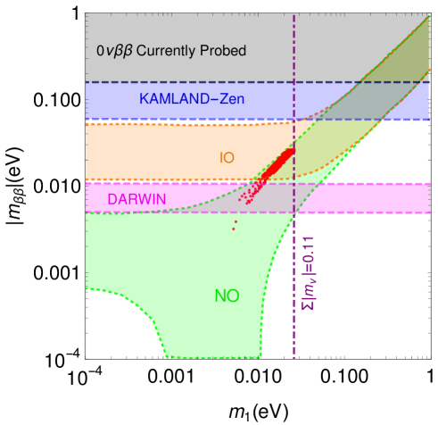
Figure 7: Prediction for $0\nu\beta\beta$ from our model for the parameter points obtained during our scan over a billion points. The absence of cancellation between different phases maximizes $|m_{\beta\beta}|$ in our model.

We have plotted our prediction for $|m_{\beta\beta}|$ in fig. 7. We have also showed the projected sensitivity of KamLAND-Zen Shirai:2017jyz and the DARWIN Agostini:2020adk experiements and our model can be probed by DARWIN. It is interesting to note that since $m_{1}\gtrsim 0.0011\,{\rm eV}$ all the light neutrino masses are nearly of same order in our model. Consequently, the third term in eq. (88) is always negligible compared to the first two terms due to the smallness of $s_{13}$ and $m_{\beta\beta}$ is dictated by the sum of the first two terms. Moreover, fig. 6 indicates that most of the solution points are concentrated in the neighbourhood of small $\alpha$ or near $\alpha=\,2\pi$, and thus no cancellation among the different contributions can take place giving $|m_{\beta\beta}|\simeq c^{2}_{13}m_{1}\approx m_{1}$, along the upper boundary of the normal hierarchy green band in fig. 7.

Since the neutrino masses are essentially generated via Type-I SeeSaw mechanism the mass eigenvalues of the heavy Majorana neutrinos in our model do not depend very strongly on the exact value of the $U(1)_{L_{\mu}-L_{\tau}}$ breaking v.e.v. $v_{D}$ or the cut-off $\Lambda$. We generally obtain heavy neutrino masses in the range $10^{-4}-1000$ GeV, so those states remain near to the EW scale.

3.2 Dark Matter Phenomenology

The phenomenology of DM has two important parts namely the production and its decay.

3.2.1 Dark Matter Production

Since the DM has very suppressed couplings, we consider again DM production via the freeze-in mechanism. But in this model, the freeze-in production of DM can take place via the decay $\phi\rightarrow\psi\bar{\psi}$ or via $2\rightarrow 2$ scatterings $\phi\phi^{\dagger}(f\bar{f})\rightarrow\psi\bar{\psi}$ through non-renormalizable operators . We shall assume that $\Phi$ is in thermal equilibrium during the cosmological evolution which is true since it mixes substantially with the SM Higgs. The decay contribution is given by Hall:2009bx :

$$Y_{\rm IR}\approx\frac{136}{4\pi^{4}}\frac{M_{Pl}}{g^{s}_{*}\sqrt{g^{\rho}_{*}}}\frac{g_{\Phi}\;\Gamma_{\Phi\rightarrow\psi\bar{\psi}}}{M^{2}_{\Phi}}\int_{x_{min}}^{\infty}\;dx\;x^{3}\;K_{1}(x)$$ (89)

where $x_{min}=M_{\Phi}/T_{RH}$. The scatterings $\phi\phi^{\dagger}(f\bar{f})\rightarrow\psi\bar{\psi}$ are mediated by the $L_{\mu}-L_{\tau}$ gauge boson $Z_{D}$. The contribution to the yield from the scatterings $ij\rightarrow\psi\bar{\psi}$ is given by,

$$Y^{ij}_{\rm UV}\approx\frac{g^{4}_{D}Q^{2}_{\psi}M_{Pl}}{\pi^{9}g^{s}_{*}\sqrt{g^{\rho}_{*}}M_{\Phi}}\int^{\infty}_{M_{\Phi}/T_{RH}}dx\int^{\infty}_{0}dy\frac{y^{3}K_{1}(y)}{(y^{2}-x^{2}M^{2}_{Z_{D}}/M^{2}_{\Phi})^{2}+x^{4}\left(M_{Z_{D}}\Gamma_{Z_{D}}/M^{2}_{\Phi}\right)^{2}}$$

$$\times\,\begin{cases}\displaystyle{y\times\frac{30\,Q^{2}_{f}}{27}}\hskip 28.45274pt{\rm when}\,ij\,\,{\rm is}\,\,f\bar{f}\\ \displaystyle{(y^{2}-4x^{2})^{3/2}\times\frac{15\sqrt{90}\,Q^{2}_{\Phi}}{256}}\\ \hskip 71.13188pt\,{\rm when}\,ij\,\,{\rm is}\,\,\Phi\Phi^{\dagger}\end{cases}\;.$$ (90)

where $\Gamma_{Z_{D}}=\dfrac{g^{3}_{D}v_{D}}{4\pi}\left(6Q^{2}_{f}+Q^{2}_{\psi}+\dfrac{Q^{2}_{\Phi}}{4}\left[1-\dfrac{4M^{2}_{\Phi}}{M^{2}_{Z_{D}}}\right]^{3/2}\right)$ is the total decay width of the gauge boson $Z_{D}$.

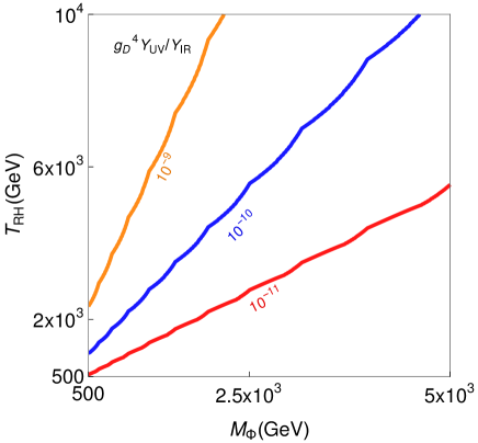
Figure 8: Left panel depicts the contours of $g^{4}_{D}Y_{UV}/Y_{IR}$ as a function of $M_{\Phi}$ and $T_{RH}$. Right panel depicts the $\Omega h^{2}=0.12$ contours in the $M_{\Phi}-f_{1}$ plane.

In order to find the relative importance of the decay and scattering process we have plotted the ratio $g^{4}_{D}Y_{UV}/Y_{IR}$ in the left-panel of fig. 8. The contribution from the scattering is negligible as long as $T_{RH}\ll M_{Z_{D}}$ since the s-channel propagator $M_{Z_{D}}$ is off-shell in this region. Moreover the presence of the $Z_{D}$ decay width in the denominator gives a $g^{-4}_{D}$ suppression in $Y_{UV}$, which is also evident in fig. 8 (left-panel). We have assumed $g_{D}$ to be 0.01 which ensures that the IR contribution is always dominant.

Thus considering only the $\phi\rightarrow\psi\bar{\psi}$ contribution we obtain:

$$\Omega_{FI}h^{2}\approx 0.1\left(\frac{f_{1}v_{D}/\Lambda}{1.51\times 10^{-9}}\right)^{2}\left(\frac{M_{\psi}}{1{\rm MeV}}\right)\left(\frac{M_{\Phi}}{1{\rm TeV}}\right)^{-1}\left[1-\frac{4M^{2}_{\psi}}{M^{2}_{\Phi}}\right]^{3/2}.$$ (91)

The contours of $\Omega_{FI}h^{2}=0.12$ are shown in the right panel of fig. 8 in the plane of $f_{1}$ and $M_{\Phi}$. As the mass of the DM increases, lower values of the coupling $f_{1}$ are required to obtain the correct relic density while $f_{1}$ can increase for increasing $M_{\Phi}$.

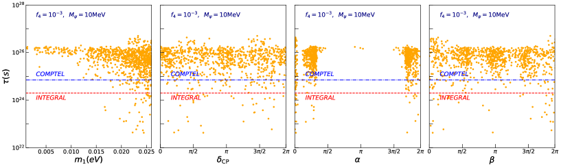
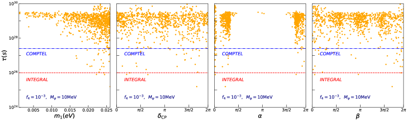
Figure 9: Prediction for DM lifetime with several neutrino physics parameters. Top panel is for the tree-level decays $\psi\rightarrow l^{+}l^{-}\nu,\nu\bar{\nu}\nu$ while bottom panel is for the loop-induced decay $\psi\rightarrow\nu\,\gamma$. In both the cases we have shown the available limit from INTEGRAL(dashed dot line) and COMPTEL(dashed line).

3.2.2 Dark Matter Decay

The DM mixes with the SM neutrinos via the mixing given in eq. (86). Thus the DM decays can occur via $\psi\rightarrow Z^{*}\nu\rightarrow f\bar{f}\nu$ or $\psi\rightarrow W^{\pm*}l^{\mp}\rightarrow f\bar{f}^{\prime}l^{\mp}$ process. The corresponding decay width is,

$$\Gamma_{\psi}^{ff\nu}\approx\left(10^{26}s\right)^{-1}\left(\frac{M_{\psi}}{1{\rm MeV}}\right)^{5}\left(\frac{|U_{\nu\psi}|}{6.345\times 10^{-12}}\right)^{2}$$ (92)

and radiative decay of the DM $\psi\rightarrow\nu\gamma$ gives,

$$\Gamma_{\psi}^{\nu\gamma}\approx\left(1.34\times 10^{30}s\right)^{-1}\left(\frac{M_{\psi}}{1{\rm MeV}}\right)^{5}\left(\frac{|U_{\nu\psi}|}{6.345\times 10^{-12}}\right)^{2}$$ (93)

The dependence of DM lifetime on several neutrino physics parameters are shown in fig. 9 for a DM mass of 10 MeV with $f_{4}=10^{-3}$. The horizontal lines are the upper limit on the DM lifetime obtained form INTEGRAL Bouchet:2008rp and COMPTEL 1999ApL&C..39..193W experiments. As we can see that most of the parameter space is beyond the reach of the present limits. In fig. 10 we have shown the constraints on the Wilson coefficient $f_{4}$ vs DM mass $M_{\psi}$ plane as obtained from INTEGRAL Bouchet:2008rp , COMPTEL 1999ApL&C..39..193W and EGRET Strong:2004de experiments. The dashed line in fig. 10 depicts the conservative limit (the weakest constraint) on $f_{4}$, whereas the solid line shows the optimistic limit i.e the possible strongest constraint. For our chosen values of $v_{D}=10^{7}\,{\rm GeV},\Lambda=10^{14}\,{\rm GeV}$ the region above the dashed line is always disallowed. The benchmark points to derive the conservative and optimistic limit are given in tab. 5. We found that the constraints on the Wilson coefficient $f_{4}$ are dominantly determined by $\psi\rightarrow e^{+}e^{-}\nu$ for $M_{\psi}>1\,{\rm MeV}$ in spite of the stronger constraints for the channel in monochromatic photons Essig:2013goa . This is mainly because for the same mixing angle the DM lifetime is nearly four orders of magnitude larger in case of the radiative decay due to the loop suppression compared to tree level decay. For a DM mass lower than 1 MeV the three body decay is not possible and only radiative decay restricts $f_{4}$. This can be seen from the right panel in fig. 10 where the DM mass starts from 40 keV.

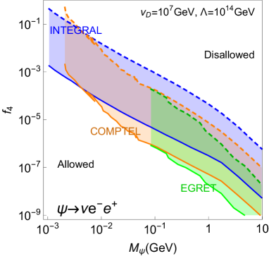
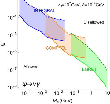
Figure 10: Constraints on the $f_{4}-M_{\psi}$ plane from INTEGRAL (Blue), COMPTEL (Orange) and EGRET (Green). The dashed lines correspond to most conservative limit and the solid lines depict the optimistic limits. The region above the dashed lines is always ruled out for $v_{D}=10^{7}\,{\rm GeV},\Lambda=10^{14}\,{\rm GeV}$.

Conservative Limit	Parameters	Optimistic Limit
0.023$\,{\rm eV}$	$m_{1}$	$0.026\,{\rm eV}$
1.46$\pi$	$\delta_{CP}$	$1.67\pi$
1.99$\pi$	$\alpha$	$0.23\pi$
1.83$\pi$	$\beta$	$1.66\pi$
$10^{-7}e^{0.049i\pi}$	$Y_{\mu}$	$10^{-7}e^{0.73i\pi}$
$10^{-7}e^{1.63i\pi}$	$Y_{\tau}$	$10^{-7}e^{1.36i\pi}$
$e^{1.5i\pi}$	$f_{6}$	$e^{0.22i\pi}$
$e^{1.1i\pi}$	$f_{7}$	$e^{1.86i\pi}$

Table 5: Neutrino oscillation parameters that gives conservative and optimistic limits on $f_{4}$ as shown in fig. 10.

3.3 Other Phenomenological Issues

• Direct Detection of DM: The DM $\psi$ carries $L_{\mu}-L_{\tau}$ charge and therefore interacts only with the second and third generation leptons. Nevertheless, it can scatter off the electrons via $\phi$ and $h$ mediated t-channel diagrams thus providing the possibility of a signal in direct detection at low energies. Following Essig:2011nj one can define a reference cross-section ($\bar{\sigma}_{e}$) and a DM form-factor ($F_{\rm DM}$) as

  $$\bar{\sigma}_{e}\, = \,\frac{\mu^{2}_{\chi e}\;y^{2}_{e}\;\theta^{2}_{h}}{2m^{4}_{\Phi}}\left(\frac{f_{1}v_{D}}{\Lambda}\right)^{2}\frac{(1+\alpha^{2}m^{2}_{e}/4m^{2}_{\chi})(1+\alpha^{2}m^{2}_{e}/4m^{2}_{e})}{\left(1+\alpha^{2}m^{2}_{e}/m^{2}_{\Phi}\right)^{2}}$$ (94)

  $$F^{2}_{\rm DM}(q)\, = \,\frac{(1+q^{2}/4m^{2}_{\chi})(1+q^{2}/4m^{2}_{e})}{\left(1+q^{2}/m^{2}_{\Phi}\right)^{2}}\times\frac{\left(1+\alpha^{2}m^{2}_{e}/m^{2}_{\Phi}\right)^{2}}{(1+\alpha^{2}m^{2}_{e}/4m^{2}_{\chi})(1+\alpha^{2}m^{2}_{e}/4m^{2}_{e})}$$

  which essentially determine the DM direct detection rate. Here $\mu_{\chi e}$ is the reduced mass of DM-electron system and $y_{e}$ is the electron Yukawa coupling. We found that even for $M_{\Phi}\simeq 10\,{\rm GeV}$ the reference cross-section $\bar{\sigma}_{e}\,\lesssim\,10^{-69}\,{\,\rm cm}^{2}$ for $\theta_{h}\,\sim\,0.1$  Such a small value of $\bar{\sigma}_{e}$ is actually two-fold suppressed: both by (i) the presence of the freeze-in coupling $f_{1}v_{D}/\Lambda$ and (ii) the electron Yukawa coupling ($y_{e}$). A target of muons or tauons would be more promising, as the Yukawa couplings are larger and also the channel with the exchange of a $Z_{D}$ gauge boson is possible, but still the expected rate is too low to be measured in future experiments.

• Electron Dipole Moment: The presence of the additional scalar $\phi$ also opens up the possibility of a new contribution to electron dipole moment(EDM) at two-loop Okawa:2019arp . The EDM contribution is given by,

  $$d^{i}_{e}=e\,L^{i}_{e}\,\int d^{4}q\,d^{4}k\,f^{i}_{\rm scalar}(q,k)$$ (96)

  where we have used $\int d^{4}q\,d^{4}k\,f^{i}_{\rm scalar}(q,k)\simeq 0.95\,M^{2}_{N,i}/m^{2}_{W}$ and

  $$L^{i}_{e}\,\simeq\,4\times 10^{-27}\,{\rm cm}\,\left(\frac{f_{3,3^{\prime}}v_{D}}{\Lambda}\right)\theta^{2}_{\nu N_{i}}\theta_{h}\frac{M_{Ni}}{m_{W}},$$ (97)

  where $\theta_{\nu N_{i}}$ is the $N_{i}-\nu$ mixing angle and $f_{3,3^{\prime}}v_{D}/\Lambda$ is the vertex factor for $N_{i}N_{i}\phi$. The smallness of the terms $f_{3,3^{\prime}}v_{D}/\Lambda\,\sim\,10^{-7}$ and $\theta_{\nu N_{i}}\,\sim\,10^{-6}$ gives an enormous suppression of order $\sim\,10^{-19}$. As a result we get $d_{e}\,\lesssim\,10^{-43}\,e\,{\rm cm}$ which is far too low compared to the latest bound from ACME ($d_{e}\,\lesssim\,10^{-29}\,e\,{\rm cm}$) Andreev:2018ayy .

• Collider constraints:

  In this model, the only dark sector fields that may appear at colliders apart from the DM are the scalar field ($\phi$) responsible for the $U(1)_{L_{\mu}-L_{\tau}}$ breaking and the heavy neutrinos ($N_{i}$) below the TeV scale. Since the scalar mixes with the SM Higgs as in portal models, we expect similar signatures in the Higgs sector, i.e. a contribution of DM to the invisible Higgs width and a modification of the Higgs couplings to the SM fermions. Also in case the scalar field is light, it may be produced via the mixing with the Higgs via gluon fusion Chang:2017ynj . For example, $\sigma(gg\rightarrow\phi)\sim 0.5{\,\rm pb}$ for $M_{\Phi}=500\,{\rm GeV}$ and $\theta_{h}=0.1$ Cepeda:2019klc .

  The heavy Majorana neutrinos couple to the SM via small neutrino Yukawa couplings and to the $\phi$ via Yukawas $h_{e\mu,e\tau}$ etc. For our choice of parameters $v_{D}=10^{7}\,{\rm GeV},\Lambda=10^{14}\,{\rm GeV}$ we obtain $h_{e\mu,e\tau}\simeq 10^{-7}$ and thus $BR(\phi\rightarrow\bar{N}N)\lesssim 10^{-9}$ even for $\theta_{h}\simeq 0.1$ and $\bar{N}N$ production rate via $\phi$-mediation is negligible at the 13 TeV LHC. On the other hand, the $pp\rightarrow h\rightarrow\bar{N}N$ is also suppressed due to the smallness of $h_{e\mu,e\tau}$ while $pp\rightarrow W^{\pm}\rightarrow\bar{N}l^{\pm}$ is negligible due to smallness of $\nu-N$ mixing $U_{\nu N}\simeq 10^{-6}$. At the LHC with $\sqrt{s}=$13 TeV, even for an integrated luminosity of $\mathcal{L}=3000\,fb^{-1}$, the number of expected $N$ events are $\simeq 0.1$(h-mediation) and $0.01$(W-mediation). If these heavy sterile neutrinos are produced, they will appear as long-lived states Cottin:2018nms ; Liu:2019ayx ; Chiang:2019ajm ,

  $$c\tau_{N}\simeq 12\,{\rm km}\left(\frac{M_{N}}{10\,{\rm GeV}}\right)^{-5}\left(\frac{U_{\nu N}}{10^{-6}}\right)^{-2}.$$ (98)

  On the other hand, in the scenario we discussed, the $Z_{D}$ gauge boson is very heavy in order to keep the dark matter state out of equilibrium, as discussed in section 3.2 and therefore does not produce signatures at colliders.

The overall advantages of this $U(1)_{L_{\mu}-L_{\tau}}$ model are:

• Non-renormalizable effective operators, suppressed by the cut-off scale $\Lambda\leq M_{Pl}$ successfully generate also in this case the effective couplings involved in DM decay as well as freeze-in in the right ballpark, without the need to fine-tune the Wilson coefficients. Moreover those operators also contribute to the neutrino masses and allow to modify the usual $U(1)_{L_{\mu}-L_{\tau}}$ predictions, lowering the sum of the neutrino masses below the present Planck constraint.

• For the lowest possible $v_{D}$ scale, an interesting cancellation among the different parameters of the neutrino mass matrix takes place, giving a correlation among the CP phases and the phases of the couplings. Unfortunately those correlations do not restrict the value of the Dirac phase, but they allow to restrict the range of the allowed effective mass for neutrinoless double beta decay, pointing to a relatively large value.

• The scenario is cosmologically consistent and anomaly free.

• The addition of the $U(1)_{L_{\mu}-L_{\tau}}$ breaking scalar $\Phi$ with the mass scale it brings in, induces mixings with the Higgs scalar and could allow the production of the new scalar state at colliders.

4 Summary and Conclusions

We have studied a set of three models in sequence, explaining the phenomenology of neutrinos and containing a decaying FIMP dark matter candidate. We focused on a fermionic DM as an example. To start with, we have considered a simple renormalizable model of SM singlet fermions which produces from the decay of a vectorlike fermion doublet $F$ while decays via Yukawa interactions with SM Higgs. The existence of the DM till today requires tiny Yukawa couplings of order $\sim 10^{-20}$ or less. Such extremely small couplings albeit ‘technically natural’ are difficult to explain, as well as the presence of very different Yukawa coupling sizes for neutrinos masses, FIMP production and DM decay.

Thus we moved to a model where the DM is charged under an additional $U(1)$ under which all SM particles are neutral. In this scenario both the DM production and decay occurs via higher-dimensional operators and thus are naturally small. These models have interesting collider signatures in terms of the vectorlike fermion decays, which explain the DM abundance in the Universe. Though this model can naturally explain the small couplings required for DM production and decay there is no direct connection between the phenomenology of the neutrino and of the DM sectors.

Next, we have attributed charges to SM leptons under the added $U(1)$. Inspired by the pattern of neutrino mixing as well as anomaly cancellation, the abelian symmetry adopted here is $U(1)_{L_{\mu}-L_{\tau}}$. We have studied this model in detail and shown that, due to the non-renormalizable operators, the neutrino mass matrix is modified. This makes is possible to satisfy the PLANCK limit on the sum of neutrino masses and at the same time obtain a sizable $0\nu\beta\beta$ rate, which could be observed in future generation experiments. DM production from the decay of the $L_{\mu}-L_{\tau}$-charged scalar $\phi$, playing in this case the role of the mother particle in FIMP production, has been computed in detail, thus eliciting constraints on the Wilson coefficients that drive DM decay.

We have also studied the possibility of DM direct detection via electron scattering and the contribution to electron dipole moment though we conclude that these effects are much lower than the reach of the future generation experiments. Implications of the neutrino physics parameters in DM decay have also been studied. Although strict correlations are yet to be identified, mostly due to the multiplicity of parameters, it is expected that further data from the neutrino sector, especially those on one or more CP-violating phases there, will serve to validate or restrict a scenario of the kind described here.

5 Acknowledgements

The work of AG and BM was partially supported by funding available from the Department of Atomic Energy, Government of India, for the Regional Centre for Accelerator-based Particle Physics (RECAPP), Harish-Chandra Research Institute. AG and BM acknowledge the hospitality of Laura Covi and the University of Göttingen where important discussions on this project took place. LC and TM thank Harish-Chandra Research Institute for visits during the work. During the initial stages of this work, LC received funding from the European Union’s Horizon 2020 research and innovation programmes InvisiblesPlus RISE under the Marie Sklodowska-Curie grant agreement No 690575 and Elusives ITN under the Marie Sklodowska-Curie grant agreement No 674896. TM is supported by a KIAS Individual Grant (PG073501) at Korea Institute for Advanced Study.

References

- (1) Planck collaboration, P. Ade et al., Planck 2015 results. XIII. Cosmological parameters, Astron. Astrophys. 594 (2016) A13, [1502.01589].
- (2) T. Banks and N. Seiberg, Symmetries and Strings in Field Theory and Gravity, Phys. Rev. D 83 (2011) 084019, [1011.5120].
- (3) Y. Mambrini, S. Profumo and F. S. Queiroz, Dark Matter and Global Symmetries, Phys. Lett. B 760 (2016) 807–815, [1508.06635].
- (4) D. Harlow and H. Ooguri, Constraints on Symmetries from Holography, Phys. Rev. Lett. 122 (2019) 191601, [1810.05337].
- (5) L. J. Hall, K. Jedamzik, J. March-Russell and S. M. West, Freeze-In Production of FIMP Dark Matter, JHEP 03 (2010) 080, [0911.1120].
- (6) N. Bernal, M. Heikinheimo, T. Tenkanen, K. Tuominen and V. Vaskonen, The Dawn of FIMP Dark Matter: A Review of Models and Constraints, Int. J. Mod. Phys. A 32 (2017) 1730023, [1706.07442].
- (7) L. Covi, J. E. Kim and L. Roszkowski, Axinos as cold dark matter, Phys. Rev. Lett. 82 (1999) 4180–4183, [hep-ph/9905212].
- (8) J. L. Feng, A. Rajaraman and F. Takayama, Superweakly interacting massive particles, Phys. Rev. Lett. 91 (2003) 011302, [hep-ph/0302215].
- (9) G. ’t Hooft, Naturalness, chiral symmetry, and spontaneous chiral symmetry breaking, NATO Sci. Ser. B 59 (1980) 135–157.
- (10) T. Asaka and M. Shaposhnikov, The MSM, dark matter and baryon asymmetry of the universe, Phys. Lett. B 620 (2005) 17–26, [hep-ph/0505013].
- (11) M. Shaposhnikov and I. Tkachev, The nuMSM, inflation, and dark matter, Phys. Lett. B 639 (2006) 414–417, [hep-ph/0604236].
- (12) M. Shaposhnikov, A Possible symmetry of the nuMSM, Nucl. Phys. B 763 (2007) 49–59, [hep-ph/0605047].
- (13) G. Arcadi and L. Covi, Minimal Decaying Dark Matter and the LHC, JCAP 08 (2013) 005, [1305.6587].
- (14) G. Arcadi, L. Covi and F. Dradi, LHC prospects for minimal decaying Dark Matter, JCAP 10 (2014) 063, [1408.1005].
- (15) S. Baek, N. Deshpande, X. He and P. Ko, Muon anomalous g-2 and gauged L(muon) - L(tau) models, Phys. Rev. D 64 (2001) 055006, [hep-ph/0104141].
- (16) C. Lam, A 2-3 symmetry in neutrino oscillations, Phys. Lett. B 507 (2001) 214–218, [hep-ph/0104116].
- (17) E. Ma, D. P. Roy and S. Roy, Gauged L(mu) - L(tau) with large muon anomalous magnetic moment and the bimaximal mixing of neutrinos, Phys. Lett. B 525 (2002) 101–106, [hep-ph/0110146].
- (18) S. Baek and P. Ko, Phenomenology of U(1)(L(mu)-L(tau)) charged dark matter at PAMELA and colliders, JCAP 10 (2009) 011, [0811.1646].
- (19) S. Baek, Dark matter and muon in local -extended Ma Model, Phys. Lett. B 756 (2016) 1–5, [1510.02168].
- (20) S. Patra, S. Rao, N. Sahoo and N. Sahu, Gauged model in light of muon anomaly, neutrino mass and dark matter phenomenology, Nucl. Phys. B 917 (2017) 317–336, [1607.04046].
- (21) W. Altmannshofer, S. Gori, S. Profumo and F. S. Queiroz, Explaining dark matter and B decay anomalies with an model, JHEP 12 (2016) 106, [1609.04026].
- (22) A. Biswas, S. Choubey and S. Khan, FIMP and Muon () in a U Model, JHEP 02 (2017) 123, [1612.03067].
- (23) A. Biswas, S. Choubey and S. Khan, Neutrino Mass, Dark Matter and Anomalous Magnetic Moment of Muon in a Model, JHEP 09 (2016) 147, [1608.04194].
- (24) A. Biswas, S. Choubey, L. Covi and S. Khan, Explaining the 3.5 keV X-ray Line in a Extension of the Inert Doublet Model, JCAP 02 (2018) 002, [1711.00553].
- (25) K. Asai, K. Hamaguchi and N. Nagata, Predictions for the neutrino parameters in the minimal gauged U(1) model, Eur. Phys. J. C 77 (2017) 763, [1705.00419].
- (26) K. Asai, K. Hamaguchi, N. Nagata, S.-Y. Tseng and K. Tsumura, Minimal Gauged U(1) Models Driven into a Corner, Phys. Rev. D 99 (2019) 055029, [1811.07571].
- (27) M. Quirós, Intermediate scales in superstring models consistent with ten-dimensional symmetries, Physics Letters B 196 (1987) 461 – 466.
- (28) R. Arnowitt and P. Nath, Intermediate mass scale in rank-six superstring models, Phys. Rev. Lett. 60 (May, 1988) 1817–1820.
- (29) R. Essig, E. Kuflik, S. D. McDermott, T. Volansky and K. M. Zurek, Constraining Light Dark Matter with Diffuse X-Ray and Gamma-Ray Observations, JHEP 11 (2013) 193, [1309.4091].
- (30) X.-D. Shi and G. M. Fuller, A New dark matter candidate: Nonthermal sterile neutrinos, Phys. Rev. Lett. 82 (1999) 2832–2835, [astro-ph/9810076].
- (31) MEG collaboration, A. Baldini et al., Search for the lepton flavour violating decay with the full dataset of the MEG experiment, Eur. Phys. J. C 76 (2016) 434, [1605.05081].
- (32) M. Cirelli, N. Fornengo and A. Strumia, Minimal dark matter, Nucl. Phys. B 753 (2006) 178–194, [hep-ph/0512090].
- (33) MoEDAL collaboration, B. Acharya et al., The Physics Programme Of The MoEDAL Experiment At The LHC, Int. J. Mod. Phys. A 29 (2014) 1430050, [1405.7662].
- (34) D. Curtin et al., Long-Lived Particles at the Energy Frontier: The MATHUSLA Physics Case, Rept. Prog. Phys. 82 (2019) 116201, [1806.07396].
- (35) J. Elias-Miro, J. R. Espinosa, G. F. Giudice, H. M. Lee and A. Strumia, Stabilization of the Electroweak Vacuum by a Scalar Threshold Effect, JHEP 06 (2012) 031, [1203.0237].
- (36) N. Okada and O. Seto, Higgs portal dark matter in the minimal gauged model, Phys. Rev. D 82 (2010) 023507, [1002.2525].
- (37) M. Lindner, D. Schmidt and T. Schwetz, Dark Matter and neutrino masses from global U(1)B−L symmetry breaking, Phys. Lett. B 705 (2011) 324–330, [1105.4626].
- (38) N. Okada and Y. Orikasa, Dark matter in the classically conformal B-L model, Phys. Rev. D 85 (2012) 115006, [1202.1405].
- (39) L. Basso, O. Fischer and J. van der Bij, Natural Z′ model with an inverse seesaw mechanism and leptonic dark matter, Phys. Rev. D 87 (2013) 035015, [1207.3250].
- (40) T. Basak and T. Mondal, Constraining Minimal model from Dark Matter Observations, Phys. Rev. D 89 (2014) 063527, [1308.0023].
- (41) B. Sánchez-Vega, J. Montero and E. Schmitz, Complex Scalar DM in a B-L Model, Phys. Rev. D 90 (2014) 055022, [1404.5973].
- (42) J. Guo, Z. Kang, P. Ko and Y. Orikasa, Accidental dark matter: Case in the scale invariant local B-L model, Phys. Rev. D 91 (2015) 115017, [1502.00508].
- (43) W. Rodejohann and C. E. Yaguna, Scalar dark matter in the BL model, JCAP 12 (2015) 032, [1509.04036].
- (44) S. Patra, W. Rodejohann and C. E. Yaguna, A new B L model without right-handed neutrinos, JHEP 09 (2016) 076, [1607.04029].
- (45) A. Biswas, S. Choubey and S. Khan, Neutrino mass, leptogenesis and FIMP dark matter in a model, Eur. Phys. J. C 77 (2017) 875, [1704.00819].
- (46) S. Okada, Portal Dark Matter in the Minimal Model, Adv. High Energy Phys. 2018 (2018) 5340935, [1803.06793].
- (47) S. Bhattacharya, N. Chakrabarty, R. Roshan and A. Sil, Multicomponent dark matter in extended : neutrino mass and high scale validity, JCAP 04 (2020) 013, [1910.00612].
- (48) G. Arcadi, T. Hugle and F. S. Queiroz, The Dark Rises via Kinetic Mixing, Phys. Lett. B 784 (2018) 151–158, [1803.05723].
- (49) Planck collaboration, N. Aghanim et al., Planck 2018 results. VI. Cosmological parameters, 1807.06209.
- (50) M. Blennow, E. Fernandez-Martinez, J. Lopez-Pavon and J. Menendez, Neutrinoless double beta decay in seesaw models, JHEP 07 (2010) 096, [1005.3240].
- (51) KamLAND-Zen collaboration, J. Shirai, Results and future plans for the KamLAND-Zen experiment, J. Phys. Conf. Ser. 888 (2017) 012031.
- (52) DARWIN collaboration, F. Agostini et al., Sensitivity of the DARWIN observatory to the neutrinoless double beta decay of 136Xe, 2003.13407.
- (53) L. Bouchet, E. Jourdain, J. P. Roques, A. Strong, R. Diehl, F. Lebrun et al., INTEGRAL SPI All-Sky View in Soft Gamma Rays: Study of Point Source and Galactic Diffuse Emissions, Astrophys. J. 679 (2008) 1315, [0801.2086].
- (54) G. Weidenspointner, M. Varendorff, K. Bennett, H. Bloemen, W. Hermsen, S. C. Kappadath et al., The Cdg Spectrum from 0.8-30 MeV Measured with COMPTEL Based on a Physical Model of the Instrumental Background, Astrophysical Letters and Communications 39 (Jan, 1999) 193.
- (55) A. W. Strong, I. V. Moskalenko and O. Reimer, Diffuse galactic continuum gamma rays. A Model compatible with EGRET data and cosmic-ray measurements, Astrophys. J. 613 (2004) 962–976, [astro-ph/0406254].
- (56) R. Essig, J. Mardon and T. Volansky, Direct Detection of Sub-GeV Dark Matter, Phys. Rev. D 85 (2012) 076007, [1108.5383].
- (57) K. Cheung, J. S. Lee and P.-Y. Tseng, New Emerging Results in Higgs Precision Analysis Updates 2018 after Establishment of Third-Generation Yukawa Couplings, JHEP 09 (2019) 098, [1810.02521].
- (58) S. Okawa, M. Pospelov and A. Ritz, Electric Dipole Moments From Dark Sectors, Phys. Rev. D 100 (2019) 075017, [1905.05219].
- (59) ACME collaboration, V. Andreev et al., Improved limit on the electric dipole moment of the electron, Nature 562 (2018) 355–360.
- (60) W.-F. Chang, T. Modak and J. N. Ng, Signal for a light singlet scalar at the LHC, Phys. Rev. D 97 (2018) 055020, [1711.05722].
- (61) M. Cepeda et al., Report from Working Group 2: Higgs Physics at the HL-LHC and HE-LHC, vol. 7, pp. 221–584. 12, 2019. 1902.00134. 10.23731/CYRM-2019-007.221.
- (62) G. Cottin, J. C. Helo and M. Hirsch, Displaced vertices as probes of sterile neutrino mixing at the LHC, Phys. Rev. D 98 (2018) 035012, [1806.05191].
- (63) J. Liu, Z. Liu, L.-T. Wang and X.-P. Wang, Seeking for sterile neutrinos with displaced leptons at the LHC, JHEP 07 (2019) 159, [1904.01020].
- (64) C.-W. Chiang, G. Cottin, A. Das and S. Mandal, Displaced heavy neutrinos from decays at the LHC, JHEP 12 (2019) 070, [1908.09838].