Equation of motion and the constraining field in ab initio spin dynamics

Abstract

It is generally accepted that the effective magnetic field acting on a magnetic moment is given by the gradient of the energy with respect to the magnetization. However, in ab initio spin dynamics within the adiabatic approximation, the effective field is also known to be exactly the negative of the constraining field, which acts as a Lagrange multiplier to stabilize an out-of-equilibrium, non-collinear magnetic configuration. We show that for Hamiltonians without mean-field parameters both of these fields are exactly equivalent, while there can be a finite difference for mean-field Hamiltonians. For density-functional theory (DFT) calculations the constraining field obtained from the auxiliary Kohn-Sham Hamiltonian is not exactly equivalent to the DFT energy gradient. This inequality is highly relevant for both ab initio spin dynamics and the ab initio calculation of exchange constants and effective magnetic Hamiltonians. We argue that the effective magnetic field and exchange constants have the highest accuracy in DFT when calculated from the energy gradient and not from the constraining field.

I Introduction

The magnetization dynamics of both insulating and metallic materials can, in many cases, be described within the framework of atomistic spin dynamics (see Refs. [1, 2] for an overview). This approach is valid when the electronic Hamiltonian can be mapped onto an effective model of localized spins with constant magnetic moment lengths and interaction parameters that are independent of the spin configuration. While this is generally fulfilled by magnetic insulators, these assumptions may not be valid for magnetic metals, for magnets with non-collinear states [3, 4], or for systems far away from equilibrium. An example of the latter is the case of ultrafast demagnetization experiments [5], where a laser pulse demagnetizes a magnetic metal on a sub-picosecond time scale. Such an extreme scenario would require a full non-equilibrium treatment of the electrons, for example with time-dependent density-functional theory (TDDFT) [6]. The numerical difficulty and computational expense of such an approach limits the applications to simulation cells with only a few atoms, which casts doubt on the ability to analyze real experiments. Therefore, it would be desirable to have a method that combines atomistic spin dynamics and electronic structure calculations with a reduced numerical complexity: ab initio spin dynamics.

Antropov et al. proposed exactly such a formalism where the torques on local magnetic moments are directly calculated from the electronic ground state energy within the adiabatic approximation [7, 8]. Stocks et al. pointed out that an arbitrary non-collinear magnetic configuration, which may be formed in such simulations, is not a stable ground state of the energy functional of density functional theory (DFT), and therefore constraining fields are needed to enforce the desired magnetization directions [9, 10]. The implementation of arbitrary constraints within DFT has been worked out previously by Dederichs et al. [11]. The use of constraining fields becomes essential for magnetic configurations that deviate strongly from that of the ground state [12].

Stocks et al. came to the conclusion that the effective field obtained from the energy gradient is exactly the negative of the constraining field, as the constraining field has to cancel the effective field [9, 10]. However, in this paper, the energy gradient and the constraining field are actually compared to confirm this relation.

Here, we present such calculations for the simple case of an iron dimer, where we find that the equivalence of the constraining field and energy gradient is not exact. Motivated by this surprising numerical result, we derive an exact relation between the constraining field and energy gradient: the constraining field theorem. This theorem shows that there is an additional term that can spoil the equality of both fields when the Hamiltonian contains mean-field parameters, which also applies to the auxiliary Kohn-Sham Hamiltonian in DFT calculations. We argue that the effective field in DFT should be calculated from the energy gradient and not the constraining field. This implies that exchange constants and effective magnetic Hamiltonians should also be derived from the energy gradient and not from the constraining field.

II Adiabatic approximation

The adiabatic approximation in ab initio spin dynamics is based on the assumption that the degrees of freedom can be separated into fast and slow components [7, 8, 13]. The slow degree of freedom is the magnetization direction, while the fast electronic degrees of freedom, including the magnetic moment lengths, are assumed to equilibrate on much shorter time scales. For the description of the magnetization dynamics, it is then valid to consider a quasi-equilibrium state where the magnetic moment directions are held fixed by Lagrange multipliers that act as constraining fields on the magnetic moments. The torques on the magnetic moments can then be calculated from this quasi-equilibrium state.

The constrained Hamiltonian is given by

$$\hat{\mathcal{H}}=\hat{\mathcal{H}}_{0}+\hat{\mathcal{H}}_{\text{con}},$$ (1)

where $\hat{\mathcal{H}}_{0}$ is the original Hamiltonian and the constraining term,

$$\hat{\mathcal{H}}_{\text{con}}=-\sum_{i}\gamma\hat{\mathbf{S}}_{i}\cdot\mathbf{B}_{i}^{\text{con}},$$ (2)

enforces a specific quasi-equilibrium state. Here, $\hat{\mathbf{S}}_{i}$ is the operator of the total spin at site $i$, the gyromagnetic ratio $\gamma=-g|e|/(2m_{e})$ with electron spin $g$-factor $g\approx 2$, and $\mathbf{B}_{i}^{\text{con}}$ is the constraining field. As shown in Fig. 1, this field, combined with intrinsic fields that are present in $\hat{\mathcal{H}}_{0}$ in Eq. (1), acts on an atomic magnetic moment,

$$\mathbf{M}_{i}=\gamma\left\langle\hat{\mathbf{S}}_{i}\right\rangle=M_{i}\mathbf{m}_{i},$$ (3)

such that the atomic moment and the constraining field are perpendicular. This causes the field to only constrain the directions of the atomic moments, $\mathbf{m}_{i}$, and not the lengths, $M_{i}$. While Eq. (2) remains finite as an operator, its expectation value vanishes,

$$\left\langle\hat{\mathcal{H}}_{\text{con}}\right\rangle=-\sum_{i}\mathbf{M}_{i}\cdot\mathbf{B}_{i}^{\text{con}}=0.$$ (4)

III Equation of motion

We consider the equation of motion of the total spin $\hat{\mathbf{S}}_{i}$ at site $i$,

$$\left\langle\dot{\hat{\mathbf{S}}}_{i}\right\rangle=\frac{i}{\text{{\hbox{\hbar}}}}\left\langle\left[\hat{\mathcal{H}}_{0},\hat{\mathbf{\mathbf{S}}}_{i}\right]\right\rangle,$$ (5)

where the expectation values have to be calculated with respect to the ground state $\psi$ of the constrained Hamiltonian $\hat{\mathcal{H}}$. In general we have for an operator $\hat{\mathcal{O}}$,

$$\left\langle\hat{\mathcal{O}}\right\rangle=\bra{\psi(\{\mathbf{e}_{i}\})}\hat{\mathcal{O}}\ket{\psi(\{\mathbf{e}_{i}\})},$$ (6)

where the ground state $\psi(\{\mathbf{e}_{i}\})$ is a function of the prescribed magnetic moment directions $\mathbf{e}_{i}$ with the expectation values of the moment directions fulfilling $\mathbf{m}_{i}=\mathbf{e}_{i}$.

The total torque on $\hat{\mathbf{S}}_{i}$ in the ground state of the full Hamiltonian in Eq. (1) is zero. This follows from

$$\left\langle\left[\hat{\mathcal{H}},\hat{\mathbf{S}}_{i}\right]\right\rangle=\left\langle E_{0}\hat{\mathbf{S}}_{i}-\hat{\mathbf{S}}_{i}E_{0}\right\rangle=0,$$ (7)

where $E_{0}$ is the ground-state energy eigenvalue of $\mathcal{H}$. This implies that for a Hamiltonian with a constraining field one may write

$$\left\langle\left[\hat{\mathcal{H}}_{\text{0}},\hat{\mathbf{S}}_{i}\right]\right\rangle+\left\langle\left[\hat{\mathcal{H}}_{\text{con}},\hat{\mathbf{S}}_{i}\right]\right\rangle=0.$$ (8)

We identify

$$\left\langle\dot{\hat{\mathbf{S}}}_{i}\right\rangle =\frac{i}{\text{$\hbar$}}\left\langle\left[\hat{\mathcal{H}}_{\text{0}},\hat{\mathbf{S}}_{i}\right]\right\rangle$$

$$=\gamma\left\langle\hat{\mathbf{S}}_{i}\right\rangle\times\mathbf{B}_{i}^{\text{eff}},$$ (9)

where $\mathbf{B}_{i}^{\text{eff}}$ is the effective field that drives the dynamics of ${\hat{\mathbf{S}}}_{i}$. Only the component of $\mathbf{B}_{i}^{\text{eff}}$ perpendicular to ${\mathbf{S}}_{i}$ contributes to the equation of motion and we define the parallel component of $\mathbf{B}_{i}^{\text{eff}}$ to be zero. By combining Eqs. (8) and (9), one obtains

$$\left\langle\dot{\hat{\mathbf{S}}}_{i}\right\rangle =-\frac{i}{\text{$\hbar$}}\left\langle\left[\hat{\mathcal{H}}_{\text{con}},\hat{\mathbf{S}}_{i}\right]\right\rangle$$

$$=\gamma\left\langle\hat{\mathbf{S}}_{i}\right\rangle\times\left(-\mathbf{B}_{i}^{\text{con}}\right),$$ (10)

which implies that the effective field

$$\mathbf{B}_{i}^{\text{eff}}=-\mathbf{B}_{i}^{\text{con}}.$$ (11)

The constraining field cancels the effective field, as illustrated in Fig. 1. This shows that the correct torque for a given Hamiltonian $\hat{\mathcal{H}}_{0}$ can be obtained from the constraining field.

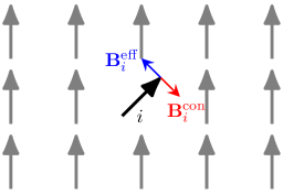
Figure 1: Effective field $\mathbf{B}_{i}^{\text{eff}}$ and constraining field $\mathbf{B}_{i}^{\text{con}}$ acting on a magnetic moment at site $i$ in a background of ferromagnetically aligned moments.

For a classical spin system with localized rigid spins (e.g., the Heisenberg model discussed in Appendix D) it can be shown that the effective field is exactly [14, 15]

$$\mathbf{B}_{i}^{\text{cl}}=-\boldsymbol{\nabla}_{\mathbf{M}_{i}}\mathcal{\mathcal{H}}_{0},$$ (12)

which would offer an alternative approach of calculating the effective field of atomistic spin-dynamics, $\mathbf{B}_{i}^{\text{eff}}$, compared to Eq. (11). However, it is not obvious that this should also hold for an itinerant magnet where the Hamiltonian is not a simple function of spin operators, but of the creation and annihilation operators of the itinerant electrons. Below we evaluate the effective field from the two approaches (11) and (12).

IV Constraining field

In the previous section we introduced the constraining field $\mathbf{B}_{i}^{\text{con}}$, but we have so far not given a procedure how to calculate this field. We know that the constraining field at site $i$ has to be tuned so that it cancels the intrinsic field of the Hamiltonian $\hat{\mathcal{H}}_{0}$ and is perpendicular to the magnetic moment direction $\mathbf{m}_{i}$. Furthermore, the constraining field has to be chosen such that at each site the moment points along the prescribed moment direction $\mathbf{e}_{i}$,

$$\mathbf{m}_{i}\overset{!}{=}\mathbf{e}_{i}.$$ (13)

We are going to consider here two methods of calculating the constraining field: the method proposed by Stocks et al. [9, 10] and the method by Ma and Dudarev [16].

Stocks et al. provide the following iterative procedure for calculating the constraining field [9, 10],

$$\mathbf{B}_{i}^{\text{con}}(k+1) =\mathbf{B}_{i}^{\text{con}}(k)-\left(\mathbf{B}_{i}^{\text{con}}(k)\cdot\mathbf{e}_{i}\right)\mathbf{e}_{i}$$

$$-B_{0}\left[\mathbf{m}_{i}-\left(\mathbf{m}_{i}\cdot\mathbf{e}_{i}\right)\mathbf{e}_{i}\right],$$ (14)

where $k$ is the iteration index and $B_{0}$ is a free parameter that can be tuned for optimal convergence. The first two terms of Eq. (14) ensure that only the contribution perpendicular to $\mathbf{e}_{i}$ is carried to the next iteration, while the third term adjusts the constraining field by a term proportional to the difference between the output and prescribed moment direction (again only keeping the perpendicular contribution), which aligns the magnetic moment $\mathbf{m}_{i}$ closer along the prescribed direction $\mathbf{e}_{i}$. The algorithm given by Eq. (14) can be derived systematically from the method of Lagrange multipliers [17]. The uniqueness of the constraining field follows from the uniqueness of the solutions within constrained DFT [18].

Ma and Dudarev derive the constraining field by imposing an energy penalty for misalignments of $\mathbf{m}_{i}$ and $\mathbf{e}_{i}$, which leads to the constraining field [16]

$$\mathbf{B}_{i}^{\text{con}}=-2\lambda\left[\mathbf{m}_{i}-\left(\mathbf{m}_{i}\cdot\mathbf{e}_{i}\right)\mathbf{e}_{i}\right],$$ (15)

where $\lambda$ determines the strength of the energy penalty and convergence is formally reached for $\lambda\to\infty$ with $\mathbf{m}_{i}\approx\mathbf{e}_{i}+\mathcal{O}(\lambda^{-1})$ [16].

Both methods look similar, but have different advantages and disadvantages. The first method (14) has the advantage of good convergence since the constraining field is adjusted step by step, but requires this additional iterative calculation, which can be done in parallel to a self-consistent calculation. The second method (15) has the advantage that it does not introduce an additional iterative calculation and can be simply included in a self-consistent calculation, but it has the disadvantage that convergence is problematic if $\lambda$ is too large. This convergence problem can be circumvented by increasing the value of $\lambda$ in steps, which keeps the energy penalty sufficiently small.

Within the formalism of constrained DFT, the constraining field can be directly included as a Lagrange multiplier in the energy minimization procedure to determine the constrained ground state [11, 19, 12, 20, 17].

V Numerical results for a dimer

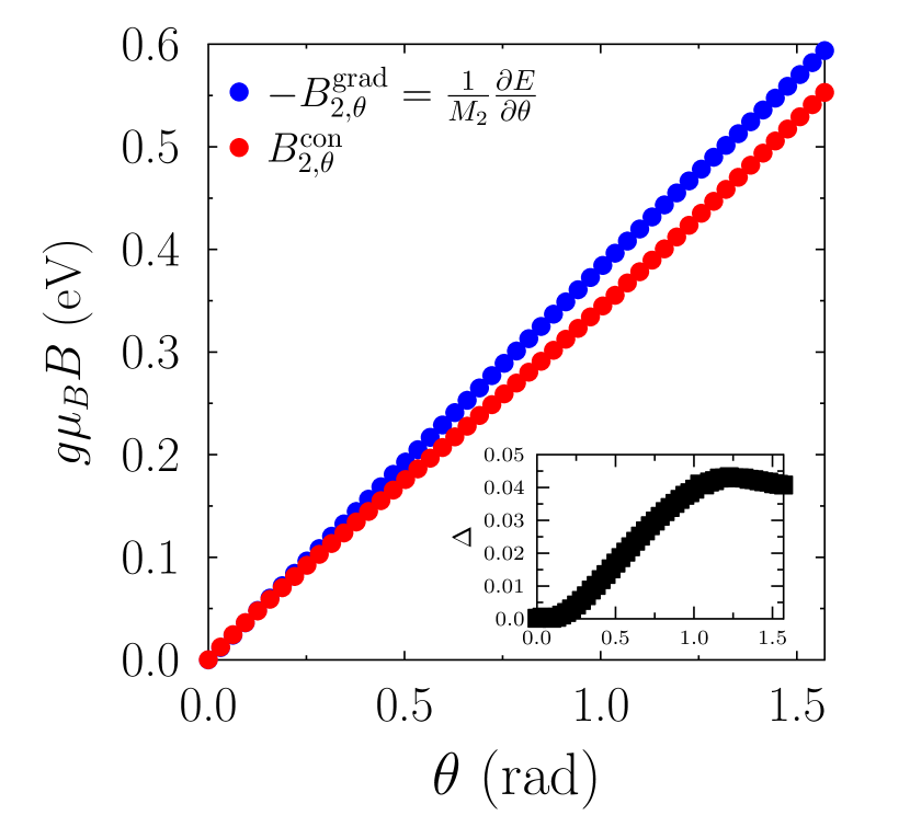
Figure 2: Comparison of the effective magnetic field calculated from the constraining field $B^{\mathrm{con}}_{2,\theta}$ (red symbols) and the energy gradient $B_{2,\theta}^{\mathrm{grad}}$ (blue symbols) for an iron dimer, where the moment $i=2$ is rotated by $\theta$. The inset shows the difference, $\Delta=-B^{\mathrm{grad}}_{2,\theta}-B^{\mathrm{con}}_{2,\theta}$, between the two effective fields.

To investigate the relation between the constraining field and the effective field obtained from the energy gradient, we performed DFT calculations for an Fe dimer system with VASP [21, 22]. The constraining field implementation in VASP is based on the method by Ma and Dudarev [16], as described above. See Appendix C for more details.

We start with both magnetic moments of the two iron atoms aligned along the $z$ axis and rotate one of the magnetic moments by an angle $\theta$ in the $xz$ plane, which gives an expression for the moment of the second atom,

$$m_{2}^{x} =\sin\theta,\;m_{2}^{y}=0,\;m_{2}^{z}=\cos\theta.$$ (16)

The effective field calculated from the energy gradient is given by

$$\mathbf{B}_{i}^{\text{grad}}=-\frac{1}{M_{i}}\boldsymbol{\nabla}_{\mathbf{e}_{i}}\left\langle\hat{\mathcal{H}}_{0}\right\rangle.$$ (17)

Since $\mathbf{e}_{i}$ is a unit vector with a fixed length, the gradient has to be defined as

$$\boldsymbol{\nabla}_{\mathbf{e}_{i}}f=\frac{\partial f}{\partial\theta_{i}}\hat{\boldsymbol{\theta}}_{i}+\frac{1}{\sin\theta_{i}}\frac{\partial f}{\partial\phi_{i}}\hat{\boldsymbol{\phi}}_{i},$$ (18)

where $\theta_{i}$ and $\phi_{i}$ are the polar and azimuthal angles in spherical coordinates with their corresponding unit vectors $\hat{\boldsymbol{\theta}}_{i}$ and $\hat{\boldsymbol{\phi}}_{i}$. The $\theta$ component of Eq. (17) is therefore

$${B}_{i,\theta}^{\text{grad}}=-\frac{1}{M_{i}}\frac{\partial}{\partial\theta_{i}}\left\langle\hat{\mathcal{H}}_{0}\right\rangle.$$ (19)

In Fig. 2, we show the $\theta$ component of the constraining field acting on the rotated spin and we compare this field to what one obtains from the energy gradient. The two calculations, Eqs. (11) and (17), are plotted in Fig. 2 as a function of $\theta$. From the figure one concludes that the two fields are similar, but not exactly identical. It is also possible to discern that the difference between them becomes bigger the further away one is from the equilibrium configuration.

For comparison, we performed analogous calculations with a mean-field tight-binding model (see Appendix A for details), which, as can be seen in Fig. 3, show similar results. There we also show the field $\tilde{\mathbf{B}}_{i}^{\text{grad}}$ which is calculated without constraining fields, with the constraints only implemented approximately by imposing local quantization axes [23] (see Appendix A). This approximate method underestimates in our case the gradient field by about 25%, even in the limit $\theta\to 0$. This implies an underestimate by 25% of the exchange parameter $J$ of the dimer in the absence of constraining fields, see Appendix D. The widely used Liechtenstein-Katsnelson-Antropov-Gubanov (LKAG) formalism [24, 25] for the calculation of exchange parameters does not take constraining fields into account [26], which could potentially result in similar inaccuracies [27].

In the following, we analyze the origin of the difference between the constraining and energy gradient fields and we argue why it matters to be aware of this difference.

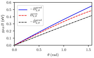
Figure 3: Comparison of the effective magnetic field calculated from the constraining field and the energy gradient for our mean-field tight-binding model applied to an iron dimer where the moment $i=2$ is rotated by $\theta$. The field $\tilde{B}_{2,\theta}^{\text{grad}}$ is calculated without constraining fields (see Appendix A).

VI Constraining field theorem

In this section, we derive the constraining field theorem, the main result of this paper, which relates the constraining field and the energy gradient field. We discuss under which circumstances these fields are equivalent and the implications this has for the correct choice of the effective field in spin-dynamics simulations.

VI.1 Derivation of the theorem

To relate the energy gradient field $\mathbf{B}_{i}^{\text{grad}}$ to the constraining field $\mathbf{B}_{i}^{\text{con}}$, we wish to evaluate $\boldsymbol{\nabla}_{\mathbf{e}_{i}}\langle\hat{\mathcal{H}}_{0}+\hat{\mathcal{H}}_{\text{con}}\rangle$. Here, and in the following, an expression

$$\boldsymbol{\nabla}_{\mathbf{e}_{i}}\left\langle\hat{\mathcal{O}}\right\rangle=\left\langle\boldsymbol{\nabla}_{\mathbf{e}_{i}}\hat{\mathcal{O}}\right\rangle+\boldsymbol{\nabla}_{\mathbf{e}_{i}}^{\psi}\left\langle\hat{\mathcal{O}}\right\rangle$$ (20)

is used, where the first term on the right-hand side accounts for the gradient of the operator $\hat{\mathcal{O}}$ and the second accounts for the gradient (or rotation) of the wavefunction $\psi$ used to calculate the expectation value. We obtain the Hellmann-Feynman theorem [28, 29],

$$\boldsymbol{\nabla}_{\mathbf{e}_{i}}\left\langle\hat{\mathcal{H}}_{0}+\hat{\mathcal{H}}_{\text{con}}\right\rangle=\left\langle\boldsymbol{\nabla}_{\mathbf{e}_{i}}\hat{\mathcal{H}}_{0}+\boldsymbol{\nabla}_{\mathbf{e}_{i}}\hat{\mathcal{H}}_{\text{con}}\right\rangle,$$ (21)

where the term that accounts for the wavefunction variation vanishes due to the extremity of the ground-state energy,

$$\boldsymbol{\nabla}_{\mathbf{e}_{i}}^{\psi}\left\langle\hat{\mathcal{H}}_{\text{0}}+\hat{\mathcal{H}}_{\text{con}}\right\rangle=0.$$ (22)

The derivative of the constraining part can be expressed as

$$\boldsymbol{\nabla}_{\mathbf{e}_{i}}\left\langle\hat{\mathcal{H}}_{\text{con}}\right\rangle=\left\langle\boldsymbol{\nabla}_{\mathbf{e}_{i}}\hat{\mathcal{H}}_{\text{con}}\right\rangle+\boldsymbol{\nabla}_{\mathbf{e}_{i}}^{\psi}\left\langle\hat{\mathcal{H}}_{\text{con}}\right\rangle.$$ (23)

Here one should note that the eigenstate that minimizes the expression in Eq. (22), does not necessarily imply that a variation over the wavefunction vanishes when one considers only $\hat{\mathcal{H}}_{\text{con}}$, i.e., $\boldsymbol{\nabla}_{\mathbf{e}_{i}}^{\psi}\langle\hat{\mathcal{H}}_{\text{con}}\rangle$ is non-zero. Similarly, both terms need to be considered when treating only $\hat{\mathcal{H}}_{0}$ in the variation,

$$\boldsymbol{\nabla}_{\mathbf{e}_{i}}\left\langle\hat{\mathcal{H}}_{0}\right\rangle=\boldsymbol{\nabla}_{\mathbf{e}_{i}}^{\psi}\left\langle\hat{\mathcal{H}}_{0}\right\rangle+\left\langle\boldsymbol{\nabla}_{\mathbf{e}_{i}}\hat{\mathcal{H}}_{0}\right\rangle.$$ (24)

Using the relationship in Eq. (22) leads to

$$\boldsymbol{\nabla}_{\mathbf{e}_{i}}\left\langle\hat{\mathcal{H}}_{0}\right\rangle=-\boldsymbol{\nabla}_{\mathbf{e}_{i}}^{\psi}\left\langle\hat{\mathcal{H}}_{\text{con}}\right\rangle+\left\langle\boldsymbol{\nabla}_{\mathbf{e}_{i}}\hat{\mathcal{H}}_{0}\right\rangle.$$ (25)

Since the moment directions for $j\neq i$ are held constant and $\mathbf{M}_{i}\cdot\mathbf{B}_{i}^{\text{con}}=0$, we find

$$-\frac{1}{M_{i}}\boldsymbol{\nabla}_{\mathbf{e}_{i}}^{\psi}\left\langle\hat{\mathcal{H}}_{\text{con}}\right\rangle=\sum_{\alpha=x,y,z}B_{i,\alpha}^{\text{con}}\boldsymbol{\nabla}_{\mathbf{e}_{i}}^{\psi}m_{i}^{\alpha}=\mathbf{B}_{i}^{\text{con}}.$$ (26)

From Eqs. (17), (25), and (26), we arrive at our main result, the constraining field theorem:

$$\mathbf{B}_{i}^{\text{grad}}=-\mathbf{B}_{i}^{\text{con}}-\frac{1}{M_{i}}\left\langle\boldsymbol{\nabla}_{\mathbf{e}_{i}}\hat{\mathcal{H}}_{0}\right\rangle.$$ (27)

For a Hamiltonian without any mean-field parameters there is no dependence on the moment directions, $\boldsymbol{\nabla}_{\mathbf{e}_{i}}\hat{\mathcal{H}}_{0}=0$, which directly implies

$$\mathbf{B}_{i}^{\text{eff}}=-\mathbf{B}_{i}^{\text{con}}=\mathbf{B}_{i}^{\text{grad}}.$$ (28)

This is analogous to the case of an effective spin Hamiltonian, given by Eq. (12), where the effective field is also given by the energy gradient.

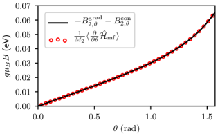
Figure 4: Numerical check of the constraining field theorem, Eq. (27), for a mean-field tight-binding model applied to an iron dimer where the moment $i=2$ is rotated by $\theta$.

VI.2 Mean-field Hamiltonians

In a mean-field treatment, the Hamiltonian $\hat{\mathcal{H}}_{\text{0}}$ is symbolized with $\hat{\mathcal{H}}_{\text{mf}}$, where the parameters of the Hamiltonian in general depend on the directions $\{\mathbf{e}_{i}\}$. In this case, the term $\langle\boldsymbol{\nabla}_{\mathbf{e}_{i}}\hat{\mathcal{H}}_{\text{mf}}\rangle$ can be finite, and it follows from Eq. (27) that the relation $\mathbf{B}_{i}^{\text{grad}}=-\mathbf{B}_{i}^{\text{con}}$ is not exact. Figure 4 shows that this term gives precisely the difference between constraining and energy gradient fields for a mean-field tight-binding calculation (see Appendix A for details), supporting the constraining field theorem (27). The difference between the two fields is determined by how strongly the mean-field parameters depend on the moment directions $\{\mathbf{e}_{i}\}$ and by how strong the correlation effects are that are represented by the mean-field contribution to $\hat{\mathcal{H}}_{\text{mf}}$. If $\hat{\mathcal{H}}_{\text{mf}}$ includes the operator-independent energy contributions arising from the mean-field decoupling, this leads to a cancellation such that $\langle\boldsymbol{\nabla}_{\mathbf{e}_{i}}\hat{\mathcal{H}}_{\text{mf}}\rangle=0$ and $\mathbf{B}_{i}^{\text{grad}}=-\mathbf{B}_{i}^{\text{con}}$, as we demonstrate in Appendix B. Such operator-independent energy contributions are not included in the tight-binding calculations shown in Figs. 3 and 4.

VI.3 Density functional theory

For the DFT calculations, we have to consider the auxiliary Kohn-Sham (KS) Hamiltonian [30] (here without spin-orbit interaction),

$$\hat{\mathcal{H}}_{\mathrm{KS}}=\sum_{l}\left[\frac{\hat{\mathbf{p}}_{l}^{2}}{2m_{e}}+V_{\mathrm{eff}}(\hat{\mathbf{r}}_{l},\hat{\mathbf{S}}_{l})\right],$$ (29)

where $l$ is the index of the KS quasiparticle with position and momentum operators $\hat{\mathbf{r}}_{l}$ and $\hat{\mathbf{p}}_{l}$ and spin operator $\hat{\mathbf{S}}_{l}$. The effective potential $V_{\mathrm{eff}}$ is not only dependent on the position and spin of the quasiparticle, but also depends on the average electron and magnetization densities, $n(\mathbf{r})$ and $\mathbf{M}(\mathbf{r})$, and we write

$$V_{\mathrm{eff}}(\hat{\mathbf{r}}_{l},\hat{\mathbf{S}}_{l})= V_{\mathrm{ext}}(\hat{\mathbf{r}}_{l})+\int\frac{n(\mathbf{r}^{\prime})e^{2}}{4\pi\varepsilon_{0}|\hat{\mathbf{r}}_{l}-\mathbf{r}^{\prime}|}\,\mathrm{d}^{3}r^{\prime}+\mu_{\mathrm{xc}}(\hat{\mathbf{r}}_{l})$$

$$-\gamma\hat{\mathbf{S}}_{l}\cdot\left[\mathbf{B}_{\mathrm{ext}}(\hat{\mathbf{r}}_{l})+\mathbf{B}_{\mathrm{xc}}(\hat{\mathbf{r}}_{l})\right],$$ (30)

where $V_{\mathrm{ext}}$ is the Coulomb potential from the ions in the lattice and $\mathbf{B}_{\mathrm{ext}}$ is an external magnetic field. The scalar and magnetic exchange-correlation potentials are given by

$$\mu_{\mathrm{xc}}(\mathbf{r})= \frac{\delta E_{\mathrm{xc}}[n,\mathbf{M}]}{\delta n(\mathbf{r})},$$ (31)

$$\mathbf{B}_{\mathrm{xc}}(\mathbf{r})= -\frac{\delta E_{\mathrm{xc}}[n,\mathbf{M}]}{\delta\mathbf{M}(\mathbf{r})},$$ (32)

where $E_{\mathrm{xc}}$ is the exchange-correlation energy, which is a functional of the electron and magnetization densities. Since these densities depend on the magnetic moment directions $\{\mathbf{e}_{i}\}$, we have $\boldsymbol{\nabla}_{\mathbf{e}_{i}}\hat{\mathcal{H}}_{\mathrm{KS}}\neq 0$ and therefore $\mathbf{B}_{i}^{\text{con}}\neq-\mathbf{B}_{i,\mathrm{KS}}^{\text{grad}}$, according to Eq. (27) applied to $\hat{\mathcal{H}}_{\mathrm{KS}}$.

It is important to note here that the constraining field theorem (27) is applied to the KS Hamiltonian and the energy gradient field $\mathbf{B}_{i,\mathrm{KS}}^{\text{grad}}$ is therefore given by the gradient of the KS energy $\langle\hat{\mathcal{H}}_{\mathrm{KS}}\rangle$ and not of the total DFT energy $E_{\mathrm{DFT}}$, which contains an additional double counting term $E_{\mathrm{dc}}$ [30, 25],

$${E}_{\mathrm{DFT}}=\left\langle\hat{\mathcal{H}}_{\mathrm{KS}}\right\rangle+E_{\mathrm{dc}}.$$ (33)

This implies for the energy gradient of the total DFT energy with Eq. (27) applied to the KS Hamiltonian,

$$\mathbf{B}_{i,\mathrm{DFT}}^{\text{grad}} =-\mathbf{B}_{i}^{\text{con}}-\frac{1}{M_{i}}\left\langle\boldsymbol{\nabla}_{\mathbf{e}_{i}}\hat{\mathcal{H}}_{\mathrm{KS}}\right\rangle-\frac{1}{M_{i}}\boldsymbol{\nabla}_{\mathbf{e}_{i}}E_{\mathrm{dc}}$$

$$=-\mathbf{B}_{i}^{\text{con}}-\frac{1}{M_{i}}\left\langle\boldsymbol{\nabla}^{*}_{\mathbf{e}_{i}}\hat{\mathcal{H}}_{\mathrm{KS}}\right\rangle,$$ (34)

where the last two terms of the first line cancel only partially and $\boldsymbol{\nabla}^{*}_{\mathbf{e}_{i}}$ denotes the variation at fixed $n(\mathbf{r})$ and $M(\mathbf{r})=|\mathbf{M}(\mathbf{r})|$. Equation (34) is the DFT adaptation of the constraining field theorem (27) and explains why the DFT calculations in Fig. 2 show a difference between the constraining and energy gradient fields.

This difference depends on the non-collinearity of the magnetization density and vanishes near the collinear limit (see Fig. 2). We can confirm this by considering that in this case the exchange-correlation field is approximately collinear within the volume $\Omega_{i}$ that is associated with the atomic site $i$,

$$\mathbf{B}_{\mathrm{xc}}(\mathbf{r})\sim\mathbf{e}_{i},\quad\forall\mathbf{r}\,\in\Omega_{i}.$$ (35)

We find

$$\left\langle\boldsymbol{\nabla}^{*}_{\mathbf{e}_{i}}\hat{\mathcal{H}}_{\mathrm{KS}}\right\rangle =-\int\left[\boldsymbol{\nabla}^{*}_{\mathbf{e}_{i}}\mathbf{B}_{\mathrm{xc}}(\mathbf{r})\right]\cdot\mathbf{M}(\mathbf{r})\,\mathrm{d}^{3}r$$

$$\sim\int_{\Omega_{i}}\mathbf{M}(\mathbf{r})\,\mathrm{d}^{3}r=\mathbf{M}_{i},$$ (36)

which does not contribute to the effective field since only components perpendicular to $\mathbf{M}_{i}$ contribute. For bulk systemsm we therefore expect that the difference between constraining and energy gradient fields will be more pronounced for short-wavelength spin waves due to their stronger non-collinearity.

VII Choice of the effective field

For a Hamiltonian $\hat{\mathcal{H}}_{0}$ with $\langle\boldsymbol{\nabla}_{\mathbf{e}_{i}}\hat{\mathcal{H}}_{0}\rangle=0$ it does not matter if the effective field is calculated from the energy gradient or the constraining field. But what is the right choice for the effective field if that is not the case, and in particular, what choice should one make in calculations based on DFT?

Let us first assume that the DFT energy $E_{\text{DFT}}$ exactly reproduces the energies of the Hamiltonian $\hat{\mathcal{H}}_{0}$, i.e,. for each configuration $\{\mathbf{e}_{i}\}$,

$$E_{\text{DFT}}=\left\langle\hat{\mathcal{H}}_{0}\right\rangle.$$ (37)

The correct effective field is then given by the DFT energy gradient,

$$\mathbf{B}_{i}^{\text{eff}}=-\frac{1}{M_{i}}\boldsymbol{\nabla}_{\mathbf{e}_{i}}\left\langle\hat{\mathcal{H}}_{0}\right\rangle=-\frac{1}{M_{i}}\boldsymbol{\nabla}_{\mathbf{e}_{i}}{E}_{\text{DFT}}=\mathbf{B}_{i,\mathrm{DFT}}^{\text{grad}},$$ (38)

which is not exactly the same as the negative of the constraining field obtained from the KS Hamiltonian, as shown by Eq. (34) and Fig. 2. This implies that the constraining field of the KS Hamiltonian $\hat{\mathcal{H}}_{\mathrm{KS}}$ is not the same as the one of the original Hamiltonian $\hat{\mathcal{H}}_{0}$ and therefore $\hat{\mathcal{H}}_{\mathrm{KS}}$ does not exactly reproduce the equation of motion,

$$\left\langle\left[\hat{\mathcal{H}}_{\mathrm{KS}},\hat{\mathbf{\mathbf{S}}}_{i}\right]\right\rangle\neq\left\langle\left[\hat{\mathcal{H}}_{0},\hat{\mathbf{\mathbf{S}}}_{i}\right]\right\rangle.$$ (39)

This is not a failure of DFT since the DFT formalism is designed to provide the correct ground state energies and electron densities. The KS Hamiltonian cannot be used to correctly describe non-equilibrium physics.

When the constraining field is not equivalent to the energy gradient, it is not exact to construct an effective magnetic Hamiltonian based on the calculation of the constraining field alone. The exchange parameters have to be calculated from the energy gradient [24, 25, 26].

If we are not considering DFT calculations and we cannot make the assumption (37), then the argument above does not apply. The effective field describing the magnetization dynamics of a given Hamiltonian $\hat{\mathcal{H}}_{0}$ is then the negative of the constraining field, as shown in Sec. III.

VIII Summary

We have shown that the effective magnetic field in the equation of motion within the adiabatic approximation is exactly the negative of the constraining field. For Hamiltonians that do not contain mean-field parameters depending on the moment directions, the effective field derived from the energy gradient is equivalent to the constraining field. We have argued that in the case of DFT the effective field should be calculated from the energy gradient because DFT is designed to reproduce the physically correct energies.

Our results have three important implications:

(1) In ab initio spin dynamics, the constraining field alone may be insufficient for calculations of the effective field, which should be obtained from the energy gradient.

(2) Therefore, exchange constants for an effective magnetic Hamiltonian also should be calculated from energy gradients and not from the constraining fields.

(3) Our tight-binding calculations support the notion that an approximate implementation of out-of-equilibrium, non-collinear states without constraining fields can give inaccurate results, even in the vicinity of the ferromagnetic ground state.

Appendix A Tight-binding model

The tight-binding model considered here is given by the Hamiltonian

$$\hat{\mathcal{H}}_{\text{tb}}=\sum_{i\alpha,j\beta,\sigma}t_{i\alpha,j\beta}\hat{c}_{i\alpha\sigma}^{\dagger}\hat{c}_{j\beta\sigma}+\hat{\mathcal{H}}_{\text{Stoner}}+\hat{\mathcal{H}}_{\text{lcn}},$$ (40)

where $\hat{c}_{i\alpha\sigma}^{\dagger}$ and $\hat{c}_{i\alpha\sigma}$ are the creation and annihilation operators of electrons at site $i$ in the orbital state $\alpha$ with spin $\sigma$. The matrix elements $t_{i\alpha,j\beta}$ are based on a Slater-Koster parametrization [32] with the parameters taken from Ref. [33]. The Stoner term is defined as

$$\hat{\mathcal{H}}_{\text{Stoner}}=\sum_{i,\alpha}\frac{I_{\alpha}}{\hbar\mu_{B}}M_{i,\alpha}\mathbf{e}_{i}\cdot\hat{\mathbf{S}}_{i,\alpha},$$ (41)

where $I_{\alpha}$ is the Stoner parameter for orbital $\alpha$, $M_{i,\alpha}$ is the moment length associated with orbital $\alpha$ at site $i$, and $\mathbf{e}_{i}$ is the prescribed moment direction. We use $I_{d}=0.96\;\text{eV}$ for the $d$ orbitals and $I_{s}=I_{p}=I_{d}/10$ for the $s$ and $p$ orbitals [34, 35]. The spin operator reads

$$\hat{\mathbf{S}}_{i,\alpha}=\frac{\hbar}{2}\sum_{\sigma\sigma^{\prime}}\boldsymbol{\sigma}_{\sigma\sigma^{\prime}}\hat{c}_{i\alpha\sigma}^{\dagger}\hat{c}_{i\alpha\sigma^{\prime}},$$ (42)

with Pauli matrix vector $\boldsymbol{\sigma}$. Charge neutrality is enforced by the term

$$\hat{\mathcal{H}}_{\text{lcn}}=U_{\text{lcn}}\sum_{i}\hat{n}_{i}\left(n_{i}-n_{i}^{0}\right),$$ (43)

where

$$\hat{n}_{i}=\sum_{\alpha,\sigma}\hat{c}_{i\alpha\sigma}^{\dagger}\hat{c}_{i\alpha\sigma}$$ (44)

counts the number of electrons at site $i$ and $n_{i}^{0}$ is the prescribed number of electrons per site. We use in our calculations $U_{\text{lcn}}=5\;\text{eV}$ [34, 35].

Both $\hat{\mathcal{H}}_{\text{Stoner}}$ and $\hat{\mathcal{H}}_{\text{lcn}}$ depend on the moment configuration $\{\mathbf{e}_{i}\}$, explicitly and via the charges $n_{i}$ and moment lengths $M_{i}$, which leads to a difference between $\mathbf{B}_{i}^{\text{grad}}$ and $-\mathbf{B}_{i}^{\text{con}}$ according to Eq. (27).

Figure 5: Comparison of the input and output moment directions $\mathbf{e}_{2}$ and $\mathbf{m}_{2}$, where the moment $i=2$ of an iron dimer is rotated by $\theta$, calculated with the tight-binding model without constraining fields.

This tight-binding model already includes an approximate implementation of the constrained moment directions $\left\{\mathbf{e}_{i}\right\}$, since these directions are favored by the Stoner term (41). Even without constraining fields, the moments align approximately along those directions. This alignment is not exact, as shown in Fig. 5, which implies that constraining fields are still required for accurate results. Our implementation of the constraining fields for the tight-binding model is based on the method by Stocks et al. [9, 10], as given by Eq. (14).

Appendix B Mean-field decoupling

Here, we demonstrate that the term $\langle\boldsymbol{\nabla}_{\mathbf{e}_{i}}\hat{\mathcal{H}}_{\text{mf}}\rangle$ vanishes when the constant energy contributions arising from the mean-field decoupling are taken into account. We consider as an example the following mean-field decoupling of a Hubbard interaction term,

$$\hat{\mathcal{H}}_{U} =U\sum_{i}\hat{n}_{i\uparrow}\hat{n}_{i\downarrow}$$

$$\approx U\sum_{i}\left(n_{i\uparrow}\hat{n}_{i\downarrow}+n_{i\downarrow}\hat{n}_{i\uparrow}-n_{i\uparrow}n_{i\downarrow}\right),$$ (45)

where the term $n_{i\uparrow}n_{i\downarrow}$ leads to the cancellation,

$$\left\langle\boldsymbol{\nabla}_{\mathbf{e}_{i}}\hat{\mathcal{H}}_{U}\right\rangle=U\sum_{i}\left[n_{i\downarrow}\boldsymbol{\nabla}_{\mathbf{e}_{i}}n_{i\uparrow}+n_{i\uparrow}\boldsymbol{\nabla}_{\mathbf{e}_{i}}n_{i\downarrow}\right.$$

$$-\left.\boldsymbol{\nabla}_{\mathbf{e}_{i}}\left(n_{i\uparrow}n_{i\downarrow}\right)\right]=0.$$ (46)

The constant energy term in Eq. (45) is required to avoid a double counting of energy contributions but does not change the dynamics of the Hamiltonian or the calculation of the constraining field.

Appendix C Numerical details

Our first principles density functional theory computations are performed with the non-collinear implementation of the VASP program package [21, 22]. The pseudopotential for Fe is considered in the generalized gradient approximation (GGA) of the projector augmented wave (PAW) method and with the cut-off energy of $600\;$eV. The valence electron configuration of the chosen Fe pseudopotential is $3d^{7}4s^{1}$. For the dimer geometry we assume a distance of $2\;\textup{\AA}$ between the atoms, which are embedded in a cubic simulation box of $8\times 8\times 8\;\textup{\AA}^{3}$. Spin-orbit coupling is neglected in our setup. The constraining field implementation in VASP is based on Ref. [16] and the Lagrange multiplier $\lambda$ of this method is typically varied in the range $10-100\;\mathrm{eV}$. Figure 2 shows the results for $\lambda=50$ which are almost indistinguishable from the results for $\lambda=100$ indicating a sufficient convergence.

Appendix D Effective spin Hamiltonians

We define here an effective spin Hamiltonian $\mathcal{H}_{\text{eff}}$ as a classical spin model which provides the energy for a given moment configuration $\left\{\mathbf{e}_{i}\right\}$. The ideal effective spin Hamiltonian would exactly reproduce the energies of the full electronic Hamiltonian in the adiabatic approximation,

$$\mathcal{H}_{\text{eff}}(\left\{\mathbf{e}_{i}\right\})=\bra{\psi(\{\mathbf{e}_{i}\})}\hat{\mathcal{H}}_{0}\ket{\psi(\{\mathbf{e}_{i}\})}.$$ (47)

Obtaining such an ideal Hamiltonian is of course in most cases impossible, as it would require one to know the energy of each configuration $\left\{\mathbf{e}_{i}\right\}$. In practice, we have to rely on simple parametrizations of $\mathcal{H}_{\text{eff}}$ that capture the relevant behavior.

For simplicity, we consider here only the Heisenberg model as an example,

$$\mathcal{H}_{\text{eff}}=-\frac{1}{2}\sum_{i,j}J_{ij}\mathbf{e}_{i}\cdot\mathbf{e}_{j},$$ (48)

which is parameterized by the exchange constants $J_{ij}$. The corresponding effective magnetic field is

$$\mathbf{B}_{i}^{\text{eff}} =-\frac{1}{M_{i}}\boldsymbol{\nabla}_{\mathbf{e}_{i}}\mathcal{H}_{\text{eff}}$$

$$=\frac{1}{M_{i}}\sum_{j}J_{ij}\left(\mathbf{e}_{j}-\mathbf{e}_{i}(\mathbf{e}_{i}\cdot\mathbf{e}_{j})\right),$$ (49)

which requires knowledge of the magnetic moment length $M_{i}$. The magnetic moment length itself may depend on the moment configuration, $M_{i}=M_{i}(\left\{\mathbf{e}_{i}\right\})$, which makes this approach only feasible if the moment length can be assumed to be constant. Here we had to subtract the component parallel to $\mathbf{e}_{i}$, which follows from the definition of the gradient (18) and the requirement that the effective field is perpendicular to $\mathbf{e}_{i}$.

For the dimer, the Heisenberg model depends only on a single exchange constant $J$,

$$\mathcal{H}_{\text{eff}}=-J\mathbf{e}_{1}\cdot\mathbf{e}_{2},$$ (50)

and the effective magnetic field is proportional to $J$,

$$\mathbf{B}_{1}^{\text{eff}} =\frac{J}{M_{1}}\left(\mathbf{e}_{2}-\mathbf{e}_{1}(\mathbf{e}_{1}\cdot\mathbf{e}_{2})\right),$$ (51)

$$\mathbf{B}_{2}^{\text{eff}} =\frac{J}{M_{2}}\left(\mathbf{e}_{1}-\mathbf{e}_{2}(\mathbf{e}_{2}\cdot\mathbf{e}_{1})\right).$$ (52)

References

- Bertotti et al. [2009] G. Bertotti, I. D. Mayergoyz, and C. Serpico, Nonlinear Magnetization Dynamics in Nanosystems (Elsevier, Oxford, 2009).
- Eriksson et al. [2017] O. Eriksson, A. Bergman, L. Bergqvist, and J. Hellsvik, Atomistic Spin Dynamics: Foundations and Applications (Oxford University Press, Oxford, 2017).
- Szilva et al. [2013] A. Szilva, M. Costa, A. Bergman, L. Szunyogh, L. Nordström, and O. Eriksson, Interatomic Exchange Interactions for Finite-Temperature Magnetism and Nonequilibrium Spin Dynamics, Phys. Rev. Lett. 111, 127204 (2013).
- Szilva et al. [2017] A. Szilva, D. Thonig, P. F. Bessarab, Y. O. Kvashnin, D. C. M. Rodrigues, R. Cardias, M. Pereiro, L. Nordström, A. Bergman, A. B. Klautau, and O. Eriksson, Theory of noncollinear interactions beyond Heisenberg exchange: Applications to bcc Fe, Phys. Rev. B 96, 144413 (2017).
- Beaurepaire et al. [1996] E. Beaurepaire, J.-C. Merle, A. Daunois, and J.-Y. Bigot, Ultrafast spin dynamics in ferromagnetic nickel, Phys. Rev. Lett. 76, 4250 (1996).
- Runge and Gross [1984] E. Runge and E. K. U. Gross, Density-functional theory for time-dependent systems, Phys. Rev. Lett. 52, 997 (1984).
- Antropov et al. [1995] V. P. Antropov, M. I. Katsnelson, M. van Schilfgaarde, and B. N. Harmon, Spin Dynamics in Magnets, Phys. Rev. Lett. 75, 729 (1995).
- Antropov et al. [1996] V. P. Antropov, M. I. Katsnelson, B. N. Harmon, M. van Schilfgaarde, and D. Kusnezov, Spin dynamics in magnets: Equation of motion and finite temperature effects, Phys. Rev. B 54, 1019 (1996).
- Stocks et al. [1998] G. M. Stocks, B. Ujfalussy, X. Wang, D. M. C. Nicholson, W. A. Shelton, Y. Wang, A. Canning, and B. L. Györffy, Towards a constrained local moment model for first principles spin dynamics, Philos. Mag. B 78, 665 (1998).
- Ujfalussy et al. [1999] B. Ujfalussy, X.-D. Wang, D. M. C. Nicholson, W. A. Shelton, G. M. Stocks, Y. Wang, and B. L. Gyorffy, Constrained density functional theory for first principles spin dynamics, J. Appl. Phys. 85, 4824 (1999).
- Dederichs et al. [1984] P. H. Dederichs, S. Blügel, R. Zeller, and H. Akai, Ground states of constrained systems: Application to cerium impurities, Phys. Rev. Lett. 53, 2512 (1984).
- Singer et al. [2005] R. Singer, M. Fähnle, and G. Bihlmayer, Constrained spin-density functional theory for excited magnetic configurations in an adiabatic approximation, Phys. Rev. B 71, 214435 (2005).
- Halilov et al. [1998] S. V. Halilov, H. Eschrig, A. Y. Perlov, and P. M. Oppeneer, Adiabatic spin dynamics from spin-density-functional theory: Application to Fe, Co, and Ni, Phys. Rev. B 58, 293 (1998).
- Landau and Lifshitz [1935] L. D. Landau and E. Lifshitz, On the theory of the dispersion of magnetic permeability in ferromagnetic bodies, Phys. Z. Sowjet. 8, 153 (1935).
- Keshtgar et al. [2017] H. Keshtgar, S. Streib, A. Kamra, Y. M. Blanter, and G. E. W. Bauer, Magnetomechanical coupling and ferromagnetic resonance in magnetic nanoparticles, Phys. Rev. B 95, 134447 (2017).
- Ma and Dudarev [2015] P.-W. Ma and S. L. Dudarev, Constrained density functional for noncollinear magnetism, Phys. Rev. B 91, 054420 (2015).
- Ivanov et al. [2020] A. V. Ivanov, P. F. Bessarab., H. Jónsson, and V. M. Uzdin, Fully self-consistent calculations of magnetic structure within non-collinear Alexander-Anderson model, Nanosyst. Phys. Chem. Math. 1, 65 (2020).
- Wu and Van Voorhis [2005] Q. Wu and T. Van Voorhis, Direct optimization method to study constrained systems within density-functional theory, Phys. Rev. A 72, 024502 (2005).
- Kurz et al. [2004] P. Kurz, F. Förster, L. Nordström, G. Bihlmayer, and S. Blügel, Ab initio treatment of noncollinear magnets with the full-potential linearized augmented plane wave method, Phys. Rev. B 69, 024415 (2004).
- Cuadrado et al. [2018] R. Cuadrado, M. Pruneda, A. García, and P. Ordejón, Implementation of non-collinear spin-constrained DFT calculations in SIESTA with a fully relativistic Hamiltonian, J. Phys. Mater. 1, 015010 (2018).
- Kresse and Furthmüller [1996] G. Kresse and J. Furthmüller, Efficient iterative schemes for ab initio total-energy calculations using a plane-wave basis set, Phys. Rev. B 54, 11169 (1996).
- Kresse and Furthmüller [1996] G. Kresse and J. Furthmüller, Efficiency of ab initio total energy calculations for metals and semiconductors using a plane-wave basis set, Comp. Mater. Sci. 6, 15 (1996).
- Grotheer et al. [2001] O. Grotheer, C. Ederer, and M. Fähnle, Fast ab initio methods for the calculation of adiabatic spin wave spectra in complex systems, Phys. Rev. B 63, 100401 (2001).
- Liechtenstein et al. [1984] A. I. Liechtenstein, M. I. Katsnelson, and V. A. Gubanov, Exchange interactions and spin-wave stiffness in ferromagnetic metals, J. Phys. F 14, L125 (1984).
- Liechtenstein et al. [1987] A. Liechtenstein, M. Katsnelson, V. Antropov, and V. Gubanov, Local spin density functional approach to the theory of exchange interactions in ferromagnetic metals and alloys, J. Magn. Magn. Mater. 67, 65 (1987).
- Bruno [2003] P. Bruno, Exchange interaction parameters and adiabatic spin-wave spectra of ferromagnets: A “renormalized magnetic force theorem”, Phys. Rev. Lett. 90, 087205 (2003).
- Jacobsson et al. [2017] A. Jacobsson, G. Johansson, O. I. Gorbatov, M. Ležaić, B. Sanyal, S. Blügel, and C. Etz, Parameterisation of non-collinear energy landscapes in itinerant magnets (2017), arXiv:1702.00599 .
- Hellmann [1937] H. Hellmann, Einführung in die Quantenchemie [English translation: Introduction to Quantum Chemistry] (Deuticke, Leipzig, 1937).
- Feynman [1939] R. P. Feynman, Forces in molecules, Phys. Rev. 56, 340 (1939).
- Kohn and Sham [1965] W. Kohn and L. J. Sham, Self-consistent equations including exchange and correlation effects, Phys. Rev. 140, A1133 (1965).
- Note [1] The result follows from the derivation in Appendix A of Ref. [25].
- Slater and Koster [1954] J. C. Slater and G. F. Koster, Simplified LCAO Method for the Periodic Potential Problem, Phys. Rev. 94, 1498 (1954).
- Thonig and Henk [2014] D. Thonig and J. Henk, Gilbert damping tensor within the breathing Fermi surface model: anisotropy and non-locality, New J. Phys 16, 013032 (2014).
- Autès et al. [2006] G. Autès, C. Barreteau, D. Spanjaard, and M.-C. Desjonquères, Magnetism of iron: from the bulk to the monatomic wire, J. Phys. Condens. Matter 18, 6785 (2006).
- Schena [2010] T. Schena, Tight-Binding Treatment of Complex Magnetic Structures in Low-Dimensional Systems, Diploma thesis, TH Aachen (2010).