Fast and Work-Optimal Parallel Algorithms for Predicate Detection

Abstract

Recently, the predicate detection problem was shown to be in the parallel complexity class NC. In this paper, we give the first work-optimal parallel algorithm to solve the predicate detection problem on a distributed computation with $n$ processes and at most $m$ states per process. The previous best known parallel predicate detection algorithm, ParallelCut, has time complexity $O(\log mn)$ and work complexity $O(m^{3}n^{3}\log mn)$. We give two algorithms, a deterministic algorithm with time complexity $O(mn)$ and work complexity $O(mn^{2})$, and a randomized algorithm with time complexity $(mn)^{1/2+o(1)}$ and work complexity $\tilde{O}(mn^{2})$. Furthermore, our algorithms improve upon the space complexity of ParallelCut. Both of our algorithms have space complexity $O(mn^{2})$ whereas ParallelCut has space complexity $O(m^{2}n^{2})$.

1 Introduction

Ensuring the correctness of distributed systems and concurrent programs is a challenging task. A bug may appear in one execution of the system, corresponding to a particular thread schedule, but not in others. One of the fundamental problems in debugging these systems is to check if the user-specified condition exists in any global state of the system that can be reached by a different thread schedule. This problem, called predicate detection, takes a concurrent computation (in an online or offline fashion) and a condition that denotes a bug (for example, violation of a safety constraint), and outputs a schedule of threads that exhibits the bug if possible [6, 1]. Predicate detection is predictive because it generates inferred reachable global states from the computation; an inferred reachable global state might not be observed during the execution of the program, but is possible if the program is executed in a different thread interleaving.

The predicate detection problem has many applications. Many classic problems in distributed computing such as termination detection, deadlock detection, and mutual exclusion can be modeled as predicate detection. Similarly, classic problems in parallel computing such as mutual exclusion violation, data race detection, and atomicity violation can also be modeled as predicate detection. General predicate detection is NP-complete [3] and therefore researchers have explored special classes of predicates. In this paper, we present improvements to the work and space complexity of parallel algorithms for the class of conjunctive predicates. While there has been extensive work in online and offline distributed algorithms for conjunctive predicate detection, there is only one parallel algorithm in the literature for predicate detection called $ParallelCut$ [9]. It is shown in [9] that:

Theorem (Garg and Garg [9]): The conjunctive predicate detection problem on $n$ processes with at most $m$ states can be solved in $O(\log mn)$ time using $O(m^{3}n^{3}\log mn)$ operations on the common CRCW PRAM.

Although this result places the predicate detection problem in the class $NC$, it has a very high work complexity of $O(m^{3}n^{3}\log mn)$. Additionally, it has a space complexity of $O(m^{2}n^{2})$. The high space complexity was required for ParallelCut as the algorithm requires the transitive closure of a matrix to achieve its fast run time. These properties make this result impractical for adoption in practice. Our results reduce both the work complexity and space complexity of solving the conjunctive predicate detection problem. Both the algorithms presented in this paper have desirable work and space complexities that make them suitable for adoption in practice. A summary of our results’ complexity measures is given in Table 1.

It should be noted that generally there are many more states along one process than there are processes in total. In essence, we should think of $m>>n$. Shaving off factors of $m$ from the work, space, and time complexities provides vast benefits in practice.

Algorithm	Work	Time	Space
Sequential [7]	$O(mn^{2})$	$O(mn^{2})$	$O(mn^{2})$
ParallelCut [9]	$O(m^{3}n^{3}\log mn)$	$O(\log mn)$	$O(m^{2}n^{2})$
This Paper: OptDetect	$O(mn^{2})$	$O(mn)$	$O(mn^{2})$
This Paper: JLSDetect	$\tilde{O}(mn^{2})$	$(mn)^{1/2+o(1)}$	$O(mn^{2})$

Table 1: Summary of previous results for conjunctive predicate detection.

We give a work-optimal parallel algorithm, OptDetect, for predicate detection. This is the first work-optimal parallel algorithm for predicate detection to the best of our knowledge. We show that the sequential algorithm presented in [9] can be parallelized and gives optimal work complexity bounds. Additionally, this algorithm can be used in an online fashion since it only looks at one state from each process per round. In the online setting, we assume that each process’s state trace is loaded into a queue and in each round we can only look at the current head of each queue. This makes it particularly useful for periodic computations or infinite computations. The work complexity guarantee of $O(mn^{2})$ matches both a lower bound on the number of operations and the sequential best shown in [7]. The lower bound argument is based on the number of comparisons it takes to find $n$ incomparable vectors in a given poset [7].

Our second result, is a fast parallel algorithm for solving the predicate detection problem. This fast algorithm, JLSDetect, gives a better time complexity bound than the current sequential best[7] and a better work complexity bound than that of ParallelCut.

In ParallelCut, one of the steps is the solving of the single-source reachability problem. This problem is widely acknowledged to have a harsh time-work trade off [10]. Parallel reachability has been studied extensively in the literature and is known to have connections to long-standing open problems in complexity theory. Until the recent breakthrough of Fineman [5], all known parallel reachability algorithms with linear work had $O(|V|)$ time complexity where $V$ is the set of vertices in the directed graph.

The JLSDetect algorithm is based off using a different reachability algorithm for this step. JLSDetect is based on the parallel reachability algorithm of Jambulapati, Liu, and Sidford [11].

In this paper, we contribute the two following theorems:

Theorem 1: The conjunctive predicate detection problem on $n$ processes with at most $m$ states can be solved by $OptDetect$ in $O(mn)$ time and $O(mn^{2})$ space using $O(mn^{2})$ operations on the common CRCW PRAM.

Theorem 2: The conjunctive predicate detection problem on $n$ processes with at most $m$ states can be solved by $JLSDetect$ in $(mn)^{1/2+o(1)}$ time and $O(mn^{2})$ space using $\tilde{O}(mn^{2})$ operations on the common CRCW PRAM with high probability in $mn$.

2 Our Model

We assume a message-passing system without shared memory or a global clock. A distributed system consists of a set of $n$ processes denoted by $P_{1},P_{2},...,P_{n}$ communicating via asynchronous messages. We assume that no messages are lost, altered or spuriously introduced. However, we do not make any assumptions about a FIFO nature of the channels. In this paper, we run our computations on a single run of a distributed system.

Each process $P_{i}$ in that run generates a single execution trace which is a finite sequence of local states. The state of a process is defined by the values of all its variables including its program counter. Let $S$ be the set of all states in the computation. We define the usual happened-before relation ($\rightarrow$) on the states (similar to Lamport’s happened-before relation between events) as follows. If state $s$ occurs before $t$ in the same process, then $s\rightarrow t$. If the event following $s$ is a send of a message and the event preceding $t$ is the receive of that message, then $s\rightarrow t$. Finally, if there is a state $u$ such that $s\rightarrow u$ and $u\rightarrow t$, then $s\rightarrow t$. A computation is simply the poset given by $(S,\rightarrow)$.

It is helpful to define what a consistent global state of a computation is. Let $s||t$ denote that states $s$ and $t$ are incomparable, i.e., $s||t\equiv s\not\rightarrow t\wedge t\not\rightarrow s$. A consistent global state $G$ is an array of states such that $G[i]$ is the state on $P_{i}$ and $G[i]||G[j]$ for all $i,j$. Consistent global states model possible global states in a parallel or a distributed computation. We assume that there is a vector clock algorithm [12, 4] running with the computation that tracks the happened-before relation. A vector clock algorithm assigns a vector $s.v$ to every state $s$ such that $s\rightarrow t$ iff $s.v<t.v$. The vectors $s.v$ and $t.v$ are called the vector clocks at $s$ and $t$. Fig. 1 shows an example of an execution trace with vector clocks.

Figure 1: State-Based Model of a Distributed Computation

A local predicate is any boolean-valued formula on a local state. For example, the predicate “$P_{i}$ is in the critical section” is a local predicate. It only depends on the state of $P_{i}$, and $P_{i}$ can obviously detect that local predicate on its own. A global predicate is a boolean-valued formula on a global state. For example, the predicate $(P_{1}\leavevmode\nobreak\ \mbox{is in the critical section})\wedge(P_{2}\leavevmode\nobreak\ \mbox{is in the critical section})$ is a global predicate. A global predicate depends upon the states of many processes. Given a computation $(S,\rightarrow)$, and a boolean predicate $B$, the predicate detection problem is to determine if there exists a consistent global state $G$ in the computation such that $B$ evaluates to true on $G$. We restrict the input so that we only consider states for which the local predicate for that process evaluates to true.

We focus on Weak Conjnctive Predicates (WCP) in this paper. A global predicate formed only by the conjunction of local predicates is called a Weak Conjunctive Predicate (WCP) [7], or simply, a conjunctive predicate. Thus, a global predicate $B$ is a conjunctive predicate if it can be written as $l_{1}\wedge l_{2}\wedge\dots\wedge l_{n}$, where each $l_{i}$ is a predicate local to $P_{i}$. We restrict our consideration to conjunctive predicates because any boolean expression of local predicates can be detected using an algorithm that detects conjunctive predicates as follows. We convert the boolean expression into its disjunctive normal form. Now each of the disjuncts is a pure conjunction of local predicates and can be detected using a conjunctive predicate algorithm. This class of predicates models a large number of possible bugs.

3 Detecting Conjunctive Predicates in Parallel

In this section, we outline some key properties used in the intuition behind predicate detection algorithms. A conjunctive predicate $B$ is of the form $B=l_{1}\wedge l_{2}\wedge\dots\wedge l_{n}$. To detect $B$, we need to determine if there exists a consistent global state $G$ such that $B$ is true in $G$. Note that given a computation on $n$ processes each with $m$ states, there can be as many as $m^{n}$ possible consistent global states. Therefore, a brute force approach of enumerating and checking the condition $B$ for all consistent global states is not feasible. Since $B$ is conjunctive, it is easy to show [7] that $B$ is true iff there exists a set of states $s_{1},s_{2},...,s_{n}$ such that (1) for all $i$, $s_{i}$ is a state on $P_{i}$, (2) for all $i$, $l_{i}$ is true on $s_{i}$ and (3) for all $i,j$: $s_{i}\|s_{j}$. Any predicate detection algorithm will either output such local states or guarantee that it is not possible to find them in the computation. When the global predicate $B$ is true, there may be multiple $G$ such that $B$ holds in $G$. For conjunctive predicates $B$, it is known that there is a unique minimum global state $G$ that satisfies $B$ whenever $B$ is true in a computation [3]. We are interested in algorithms that return the minimum $G$ that satisfies $B$ since the minimum $G$ corresponds to the smallest counter-example to a programmer’s understanding.

4 OptDetect: A Work-Optimal Deterministic Algorithm for Predicate Detection

function OptDetect() Input: $states:array[1\dots n][1\dots m]$ of vectorClock; // sequence of local states given by vector clocks Output: Consistent Global State as array $cut[1\dots n]$ Step 1: Create $cut$: set of initial states var $cut:array[1\dots n]$ of vectorClock; var $current:array[1\dots n]$ of $\{1\dots m\}$ for $i:=1$ to $n$ in parallel do $current[i]:=1$ ; $cut[i]:=states[i,current[i]]$ ; Step 2: Create $color$: array[$1$..$n$] of $\{red,green\}$; var $color:array[1\dots n]$ of $\{red,green\}$ init $green$ for all ($i\in 1\dots n,j\in 1\dots n)$ in parallel do if $cut[i]\rightarrow cut[j]$ then $color[i]:=red$; Step 3: Advance $cut$ in parallel for all $(i\in 1\dots n)$ in parallel do if $color[i]=red$ then if $cut[i]$ is the last state on its process then output("No satisfying Consistent Cut"); else $current[i]:=current[i]+1$; $cut[i]:=states[i,current[i]]$; $color[i]$ := $green$; for $j:=1$ to $n$ in parallel do if $(color[j]=green)$ then if $(cut[i]\rightarrow cut[j])$ then $color[i]:=red$; if $(cut[j]\rightarrow cut[i])$ then $color[j]:=red$; endfor; endfor; return $ConsistentCut:=cut$ ; Figure 2: The OptDetect algorithm to find the first consistent cut.

In this section, we give the OptDetect algorithm. The OptDetect algorithm is the parallelization of the serial conjunctive predicate detection algorithm, SequentialCut, presented in [9].

At a high level, we initialize the cut to the set of first states on each process. After this, we see if this cut contains states that are all concurrent with each other. If this is the case, we are done. If some states happened-before other states in this cut, we advance along those processes in parallel. We then re-evaluate our current cut to see if all states are concurrent with each other. This procedure repeats until we arrive at the first consistent cut.

Since OptDetect is the paralleliztion of the SequentialCut algorithm, correctness follows from [9]. What remains to be shown are the time and work bounds.

In step one of OptDetect, we declare and initialize cut and current in constant time using $n$ processors. The data structures cut and current will be used to hold the current global state of the system and the index we are currently at on each process respectively. Thus, step one takes $O(n)$ operations. In step two, we declare and initialize color which will be used to identify which states are “bad”. This tells us that we must advance on the processes that these states lie on. Step two takes $O(n^{2})$ work since we use $O(n^{2})$ processors and executing this step takes $O(1)$ time. In step three, we advance cut in parallel to the first satisfying consistent cut. To analyze the time and work for this step, let us see how we color the states. Once a state has been colored red, we advance along that state and never consider it again. Since there are at most $mn$ states, we consider at most $mn$ states. Each time we consider a state to be in the first consistent cut, we have to make $O(n)$ comparisons to the other $n-1$ states in cut. So, in total, this step takes $O(mn^{2})$ work. In the worst case we must explore all states to find the first consistent cut, so the time complexity is $O(mn)$. It should be noted that we get a time complexity of $O(mn)$ only in the pathological case where we only reject one state every time we advance on a process. Often, this algorithm will perform much better than $O(mn)$. Since this algorithm has been broken down into steps, we just have to identify the steps that have the largest time and work complexities. In this case, step three has both the largest time and work complexity of $O(mn)$ and $O(mn^{2})$ respectively.

Notice that this algorithm can be used in an online fashion since it only looks at one state from each process per round. In the online setting, we assume that each process’s state trace is loaded into a queue and in each round we can only look at the current head of each queue. This makes it useful for applications that require periodic computations or infinite computations.

Lastly, notice that we only ever use the states input of vector clocks and no data structure larger than states. So, the space complexity of OptDetect is $O(mn^{2})$ since there are at most $mn$ states and each is identified by a vector clock of size $O(n)$.

In Figure 2, we give the OptDetect algorithm that solves the predicate detection problem in $O(mn)$ time using $O(mn^{2})$ operations on the common CRCW PRAM.

5 JLSDetect: A Fast Randomized Algorithm for Predicate Detection

Next, we describe the second algorithm, JLSDetect. JLSDetect is based loosely around the idea of computing reachability of rejected states in the state rejection graph of a distributed system. This idea is presented in [9]. In Figure 3, we show what the state rejection graph looks like for the given computation in Figure 1.

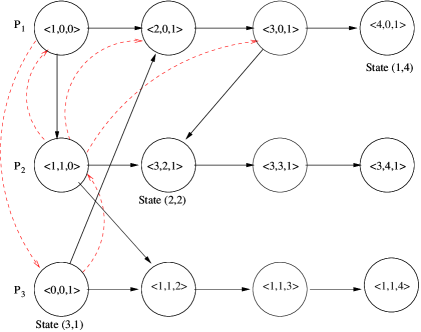
Figure 3: State Rejection Graph of a computation shown in dashed arrows

JLSDetect improves upon the space complexity of ParallelCut by using a smaller modified data structure to represent to represent the state rejection graph. We are able to get a strong time complexity guarantee of $(mn)^{1/2+o(1)}$. This is because we use the parallel reachability algorithm presented in [11]. From here on, we will refer to this parallel reachability algorithm due to [11] as JLSReach.

At a high level, JLSReach is actually taking in a graph with $|V|$ vertices and adding shortcut edges to reduce the diameter to $|V|^{1/2+o(1)}$ $w.h.p$. After this is done, the traditional ParallelBFS can be utilized since ParallelBFS runs in linear work and time proportional to the diameter of the graph. The output after reducing the diameter and running ParallelBFS is the set of nodes reachable from a specified source node $s$ in the diameter-reduced graph $G$. For a more detailed explanation of the algorithm, we refer the reader to [11].

In ParallelCut, the algorithm uses a state rejection graph of size $mn$ by $mn$ to compute the consistent cut. The state rejection matrix allows us to query two states $s$ and $s^{\prime}$ and tells us if the rejection of state $s$ implies the rejection of state $s^{\prime}$. A more detailed explanation of the state rejection graph is given in [9].

To reduce the space complexity, we want to reduce the representation size of the state rejection graph. To do this, we exploit the structure of the predicate detection problem to create a modified incidence matrix that represents the state rejection graph. The state rejection graph, $R$, is now represented as a smaller incidence matrix instead of as an adjacency matrix. We call this incidence matrix the state-max incidence matrix. The state-max incidence matrix is smaller due to the following observation.

Notice that each state has at most $n$ edges to other states in the state rejection graph. Consider the state-based representation corresponding to a single run of a distributed system. If some state $s=(i,j)$ has multiple edges in the graph such that these edges point to states on the same processor, we only need to consider the edge that points to the state with largest $j$ value, say state $s^{\prime}=(i^{\prime},j^{\prime})$. This is because the rejection of state $s$ implies the rejection of state $s^{\prime}$ but also implies the rejection of all states that happened-before state $s^{\prime}$. Trivially, this includes all states that happened-before state $s^{\prime}$ and are on the same process as $s^{\prime}$.

This allows us to only use a matrix indexed by states on one axis and by processors on the other axis. Now, our state-max incidence matrix is of size $O(mn^{2})$. Instead of explicitly, writing out each state on one axis of the matrix, we can use pointers to point back to the corresponding states in the input states. For each state, we keep track of the largest state along all other processors for which it has an edge pointing to that state. More formally, we populate $R$ as follows:

$$R[(i,j),i^{\prime}]=j^{\prime}\equiv((i^{\prime},j^{\prime})\rightarrow(i,j+1)\wedge(\nexists\leavevmode\nobreak\ (i^{\prime},j^{\prime\prime})\leavevmode\nobreak\ |\leavevmode\nobreak\ (j^{\prime\prime}>j)\wedge(i^{\prime},j^{\prime\prime})\rightarrow(i,j+1)))$$

function JLSDetect() Input: $states:array[1\dots n][1\dots m]$ of vectorClock // Sequence of local states at each process Output: Consistent Global State as array $cut[1\dots n]$ Step 1: Create $F$: set of states rejected in the first round var $F:array[1\dots n]$ of $0\dots 1$ initially $0$; for all $(i\in 1\dots n,j\in 1\dots n)$ in parallel do if $((i,1)\rightarrow(j,1))$ then $F[i]:=1$; Step 2: Create $R$: State Rejection Graph // Represented as a State-Max Incidence Matrix var $R:[(1\dots n,1\dots m),(1\dots n)]$ of $0\dots m$ for all $(i\in 1\dots n,j\in 1\dots m,i^{\prime}\in 1\dots n)$ $R[(i,j),i^{\prime}]=0$ for all $(i\in 1\dots n,j\in 1\dots m)$ in parallel do $R[(i,j),i]=j$; for all $(i\in 1\dots n,j\in 1\dots m-1)$ in parallel do for $(i^{\prime}\in 1\dots n)$ in parallel do $loadVector=states[i][j+1];$ $R[(i,j),i^{\prime}]=loadVector[i^{\prime}]$; Step 3: Create $RR$: set of nodes reachable from $F$ using $R$ var $RR:array[(1\dots mn)]$ of $0\dots 1$ $V(R):=V(R)\cup\{f\}$ $E(R):=E(R)\cup E_{f}$ $RR=JLSReach(R,f)$ Step 4: Create $valid$: replace invalid states by $0$ var $valid:array[[1\dots n][1\dots m]$ of $0\dots 1$; for all $(i\in 1\dots n,j\in 1\dots m)$ in parallel do $valid[i][j]:=1$; for all $(i\in 1\dots n,i^{\prime}\in 1\dots n,j^{\prime}\in 1\dots m)$ in parallel do if $(F[i]=1)\wedge(RR[(i^{\prime},j^{\prime})]=1)$ then $valid[i^{\prime}][j^{\prime}]:=0$; Step 5: Create $cut$: First Consistent Global State var $cut:array[1\dots n]$ of $0\dots m$ initially 0; for all $(i\in 1\dots n,j\in 1\dots m)$ in parallel do if $(valid[i][j]\neq 0)$ then if $(j=1)\vee((j>1)\wedge(valid[i][j-1]=0)$ then $cut[i]:=j$; for all $(i\in 1\dots n)$ in parallel do if $(cut[i]=0)$ then output("No satisfying Consistent Cut"); return $ConsistentCut:=cut$; Figure 4: The JLSDetect algorithm to find the first consistent cut.

Populating this state-max incidence matrix can be done in $O(1)$ time since the relation we have described above is exactly what is stored in the vector clock representation of a state. If some state $s$ has vector clock $\vec{v_{s}}=[s_{1},s_{2},\dots,s_{n}]$, then by the definition of vector clock, $s_{i}$ is the largest process on process $i$ that happened-before $s$. So, to set the the state-max incidence matrix, we will, for state $s=(i,j)$, load in the vector clock of state $s^{\prime}=(i,j+1)$ into $R$ such that $R[(i,j),i^{\prime}]=\vec{{v_{s^{\prime}}}}[i^{\prime}]$. By using a separate processor for each state, and then $n$ processors to load in the vector clock, this can be done in $O(1)$ time and $O(mn^{2})$ work.

The improved time complexity bound comes directly from the time complexity of computing reachability using JLSReach. For any $|V|$-node $|E|$-edge directed graph, JLSReach computes all vertices reachable from a given source node $s$ with $\tilde{O}(|E|)$ work and $|V|^{1/2+o(1)}$ time with high probability in $|V|$. Since we have at most $mn$ nodes in our state rejection graph and we know there are at most $mn^{2}$ edges in the state rejection graph, the work complexity and time complexity of using JLSReach is $\tilde{O}(mn^{2})$ and $(mn)^{1/2+o(1)}$ respectively.

Now, we will informally explain the steps of the algorithm.

In step one, we create $F$, the set of all initially rejected states. Let $I$ be the global state consisting of each processor’s first local state, i.e., $I=\{(i,1)\leavevmode\nobreak\ |\leavevmode\nobreak\ i\in 1..n\}.$ If there are no dependencies between any of these states, we have already reached the first consistent global state. Else, if there is a dependency from one of these states to another, we reject whichever state happened-before the other and add it to $F$. We represent the set $F$ by a boolean bit array of size $n$ that is indexed by processor. This step can be done in $O(1)$ time in parallel with $O(n^{2})$ work by using a separate processor for each value of $i$ and $j$.

In step two, we create the state rejection graph $R$ as a state-max incidence matrix following the procedure given above.

In step three, we run JLSReach on $R$. Notice that to use JLSReach in step three, we must have a $single$ source node $s$. However, in our algorithm, $F$ may contain multiple nodes. Instead of running JLSReach from each node in $F$, we can introduce a dummy source node $f$. We add the following set $E_{f}$ of edges to our state rejection graph:

$$E_{f}=\{<f,v>\leavevmode\nobreak\ |\leavevmode\nobreak\ v\in F\}$$

Now, we can run JLSReach on $R$ from $f$ and this returns the set $RR$ of all vertices reachable from nodes in $F$ in the state rejection graph. In our given implementation, we use a Boolean bit array to represent set membership in $RR$.

In step four, we mark which states are valid by using both $F$ and $RR$. A valid state is one that is part of a consistent cut. This step sets rejected states, or invalid states, with a $0$. This step can also be done in $O(1)$ time and $O(mn^{2})$ work.

Lastly, in step five, we find the first consistent global state. To do this, we will look at our previous data structure valid, and find the invalid state with the largest $j$ index along each process. Let this largest invalid state along process $p_{i}$ be $s=(i,j)$. Then, the first consistent global state contains the state $(i,j+1)$, namely, the state that appears right after state $s$. Of course, if the largest invalid state is the last state along a process, there does not exist a consistent global state. To compute the index of the largest invalid state, we will use a divide-and-conquer parallel reduce algorithm. For more on the parallel reduction operator, see [2].

Let’s treat the sequence of states along each process as a 0-1 array where we have 0’s as invalid states and 1’s as valid states. To find the largest invalid state, i.e. the $0$-entry with the largest index, we will split the array into two halves and ask each half to compute its largest invalid state. Then, we give priority to the half that appears further on in the array. We continue splitting up these arrays until we are left with two entries. From here, we can simply compare the two entries and return index of the largest $0$. If neither entry has a $0$, we will return $0$. This process takes $O(\log m)$ rounds. Each round can be computed in $O(1)$ time if we have $O(mn)$ processors. So, this step takes $O(\log m)$ time and $O(mn)$ work. The recursive procedure to find this largest invalid state along each process is called function FLIS and is given in Figure 5. FLIS is used as a subroutine in JLSDetect.

function FLIS() Input: $S:array[1\dots m]$ of $0\dots 1$, start index, end index; // Sequence of local states’ validity given by $0$-$1$ Output: Index of largest 0 entry in $p_{i}$-$states$ if $(end$ - $start==1)$ if$(S[start]==0\wedge S[end]==1)\leavevmode\nobreak\$ return $start$; if$(S[start]==0\wedge S[end]==0)\leavevmode\nobreak\$ return $end$; if$(S[start]==1\wedge S[end]==0)\leavevmode\nobreak\$ return $end$; if$(S[start]==1\wedge S[end]==1)\leavevmode\nobreak\$ return $0$; else return $max(FLIS(S,start,end/2),FLIS(S,1+end/2,end))$; Figure 5: The FLIS subroutine to find the first the largest invalid state along a process $p_{i}$.

Now, that we have the largest invalid state along each process, we can compute the first consistent global state by taking the successor of each of these states. This takes $O(1)$ time with $O(n)$ processors.

Computing the time and work complexity of this algorithm boils down to finding the individual steps with the highest time and work costs. In this case, step three takes the longest time with a time cost of $(mn)^{1/2+o(1)}$. The step with the largest work cost is also step three with a work cost of $\tilde{O}(mn^{2})$ where $\tilde{O}(g(n))$ hides polylogarithmic factors in the function $g(n)$. Notice that the work-complexity is only off of the optimal by a $polylog(mn)$ factor. Similar to OptDetect, the correctness of this algorithm follows from [9] since we have only replaced one reachability method with another. It is important to note that JLSDetect is a randomized algorithm. JLSDetect is given in Figure 4.

6 Conclusions and Future Work

We have given two algorithms which improve upon the best known parallel predicate detection algorithms in terms of work complexity and space complexity. We give the first work-optimal parallel algorithm for conjunctive predicate detection. Additionally, we give a fast randomized parallel predicate detection algorithm that outperforms the current sequential best and offers good work complexity guarantees. Both the algorithms presented in this paper have properties that make them suitable for adoption in practice.

Recently, it was shown that many classical combinatorial optimization problems such as the stable marriage problem, market clearing price problem, and shortest-path problem can be cast as searching for an element that satisfies an appropriate predicate in a distributive lattice [8]. Finding quicker predicate detection algorithms with strong work complexity guarantees is an open work with applications to this framework and potentially many other classic optimization problems.

An open question that remains is: does there exist a parallel conjunctive predicate detection algorithm that runs in $O(polylog(mn))$ time using $O(mn^{2})$ operations? An algorithm with these properties would lie in the parallel complexity class NC and be work-optimal.

7 Acknowledgements

The author would like to thank Vijay Garg for many helpful comments and discussions on this work.

References

- [1] Özalp Babaoğlu and Keith Marzullo. Consistent Global States of Distributed Systems: Fundamental Concepts and Mechanisms, page 55–96. ACM Press/Addison-Wesley Publishing Co., USA, 1993.
- [2] Guy E. Blelloch and Bruce M. Maggs. Parallel algorithms. In Mikhail J. Atallah, editor, Algorithms and Theory of Computation Handbook, Chapman & Hall/CRC Applied Algorithms and Data Structures series. CRC Press, 1999. doi:10.1201/9781420049503-c48.
- [3] C. Chase and V. K. Garg. Efficient detection of global predicates in a distributed system. Distributed Computing, 11(4), 1998.
- [4] C. J. Fidge. Partial orders for parallel debugging. Proceedings of the ACM SIGPLAN/SIGOPS Workshop on Parallel and Distributed Debugging, published in ACM SIGPLAN Notices, 24(1):183–194, January 1989.
- [5] Jeremy T. Fineman. Nearly work-efficient parallel algorithm for digraph reachability. In Proceedings of the 50th Annual ACM SIGACT Symposium on Theory of Computing, STOC 2018, page 457–470, New York, NY, USA, 2018. Association for Computing Machinery. doi:10.1145/3188745.3188926.
- [6] V. K. Garg. Elements of Distributed Computing. Wiley & Sons, 2002.
- [7] V. K. Garg and B. Waldecker. Detection of weak unstable predicates in distributed programs. IEEE Transactions on Parallel and Distributed Systems, 5(3):299–307, March 1994.
- [8] Vijay K. Garg. Predicate detection to solve combinatorial optimization problems. In Proceedings of the 32nd ACM Symposium on Parallelism in Algorithms and Architectures, SPAA ’20, page 235–245, New York, NY, USA, 2020. Association for Computing Machinery. doi:10.1145/3350755.3400235.
- [9] Vijay K. Garg and Rohan Garg. Parallel algorithms for predicate detection. In Proceedings of the 20th International Conference on Distributed Computing and Networking, ICDCN ’19, page 51–60, New York, NY, USA, 2019. Association for Computing Machinery. doi:10.1145/3288599.3288604.
- [10] Richard M. Karp and Vijaya Ramachandran. Parallel Algorithms for Shared-Memory Machines, page 869–941. MIT Press, Cambridge, MA, USA, 1991.
- [11] Yang P. Liu, Arun Jambulapati, and Aaron Sidford. Parallel reachability in almost linear work and square root depth. In David Zuckerman, editor, 60th IEEE Annual Symposium on Foundations of Computer Science, FOCS 2019, Baltimore, Maryland, USA, November 9-12, 2019, pages 1664–1686. IEEE Computer Society, 2019. doi:10.1109/FOCS.2019.00098.
- [12] F. Mattern. Virtual time and global states of distributed systems. In Parallel and Distributed Algorithms: Proc. of the International Workshop on Parallel and Distributed Algorithms, pages 215–226. Elsevier Science Publishers B.V. (North-Holland), 1989.