An optimal linear filter for estimation of random functions in Hilbert space
Abstract
Let be a square-integrable, zero-mean, random vector with observable realizations in a Hilbert space , and let be an associated square-integrable, zero-mean, random vector with realizations, which are not observable, in a Hilbert space . We seek an optimal filter in the form of a closed linear operator acting on the observable realizations of a proximate vector that provides the best estimate of the vector . We assume the required covariance operators are known. The results are illustrated with a typical example.
2020 Mathematics subject classification: Primary: 49J55, Secondary: 49K45, 60K40
Keywords and phrases: random functions, optimal estimation, linear operators, generalized inverse operators
1 Introduction
A common problem in engineering, applied mathematics and statistics is the estimation of a random function , whose realizations are not observable, by using the observable realizations of an associated random function . We consider the following problem.
Problem 1.1
Let be a probability space, and Hilbert spaces, and and square-integrable, zero-mean, random functions with respective observable and unobservable realizations and for each outcome . Find a closed, densely defined, linear operator , a proximate observable function for each with and for -almost all , and a corresponding estimate of the unobservable function, such that
| (1) |
is minimized.
For each outcome the realization of the error function is an element of the Hilbert space . The value is the square of the magnitude of the pointwise error. The estimated overall error in (1) is the mean or expected value of the square of the magnitude of the pointwise error. The proximate observable function must be close to the observable function in the sense that the mean square observation error must be small. The outcomes must lie in the domain space of the operator for -almost all . The pointwise estimate of the unobservable function is defined by for each . The linear operator does not depend on the approximation parameter . We use the terms random vector and random function interchangeably, but for the most part, prefer the latter.
We assume that the key covariance operators, the auto-covariance and the cross-covariance , are known bounded linear operators. We expect to find a solution in the form where and is the generalized inverse auto-covariance operator and this perception enables us to identify some critical issues. The auto-covariance operator is positive semi-definite, self-adjoint and compact. Therefore the spectral set is reduced to a countable collection of real non-negative eigenvalues. When there are an infinite number of positive eigenvalues the auto-covariance is not bounded below and the range space is not a closed subspace. Therefore the generalized inverse auto-covariance is an unbounded linear operator. Consequently the proposed solution is also unbounded. Now there are two specific issues that must be resolved.
In the first instance the usual justification for the solution assumes that the auto-covariance of the transformed observable function is given by the formula . The usual justification is no longer valid if the operator is unbounded. The matter is resolved by writing where is a bounded linear operator and then using an alternative argument to find an optimal value for .
In the second instance a solution in the form would require the observable function to lie in the domain of the unbounded operator . This cannot be guaranteed. The difficulty can be resolved by introducing a proximate observable function , for each , which must lie in the domain of but needs to be close to in the sense that the mean square error in the observed values satisfies . The proposed solution now takes the form . This raises a further question. How can we ensure that the operator—which does not depend on the approximation parameter—is still optimal for the proximate function? The answer is found by taking the proximate function as a partial sum of the Fourier series for the observable function.
1.1 A basic formulation of the problem.
Let denote a probability space where is the set of outcomes, a complete -field of measurable subsets and an associated probability measure on , with . Each element represents the outcome of an observation or experiment and each is a set of outcomes, called an event. We say that the event has occurred if . Let and be complex-valued random vectors with zero mean. That is, we assume
We would like to estimate from a knowledge of . One might postulate a linear relationship in the form where is an unknown matrix and is a random error vector which is independent of and has zero mean. If so then after realizations one would obtain a system of equations
| (2) |
where we have written , , where is the outcome of the experiment and where , and . In general, because we have merely postulated a linear relationship, one would not expect this equation to be satisfied exactly. Thus we seek to minimize the mean-square error . Hence we solve the system
| (3) |
We make a probabilistic interpretation of this equation by noting that
| (4) |
and
| (5) |
where is the expectation operator and and are the standard auto-covariance and cross-covariance matrices for zero-mean vectors. Thus we rewrite the equation for the best estimate of in the form
| (6) |
1.2 The definitive properties of the covariance matrices.
To extend the above analysis to random vectors in Hilbert space we must be able to define appropriate covariance operators. Notice that
for each and
for each and and also that
where is the expectation operator. By taking the limit as the number of independent realizations tends to infinity we obtain the basic theoretical relationships
| (7) | |||||
| (8) | |||||
| (9) |
for all and . We will take these as the definitive properties of the covariance operators for the random vectors and .
1.3 A typical application—input retrieval in a linear system.
We illustrate our theoretical results by considering the problem of input retrieval in an infinite-dimensional linear system. Our formal task is to find an optimal estimate of the system input from observations of the system output. The input is a random function which is represented as a Fourier series with random coefficients. The output is a random function where each realization of the output is uniquely determined by the corresponding realization of the input for some . We assume there is no independently generated noise to disrupt our observations of the output. This makes no substantial difference to the methodology. The introduction of noise simply decreases the accuracy of the estimation. In our hypothetical example we consider a known system so that the required covariance operators and are also known. In practice it may be necessary to estimate these operators a priori in a controlled experiment. Each observed output is approximated by a truncated Fourier series for some fixed and the input is then estimated using the formula . See also [12] for an application to input retrieval in finite-dimensional linear control systems and [4, Section 8.4.1, pp 261–262] for the extension of these ideas to infinite-dimensional systems.
Our hypothetical example is a special case of a more general collection of so-called inverse problems. See Cotter et al. [6] for an extended discussion of the underlying statistical theory of optimal estimation and a collection of particular inverse problems arising from data assimilation in fluid mechanics. In each application one assumes that the system evolves in a predominantly deterministic manner from some unknown initial configuration and that the evolution is monitored either directly or indirectly by observation of various output signals that may or may not be disrupted by random noise. The objective is to make inference about the underlying velocity field. For problems without model error the inference is on the initial conditions. For problems with model error the inference is on the initial conditions and on the driving noise process or, equivalently, on the entire time-dependent velocity field. Cotter et al. [6] illustrate their theoretical results by considering the velocity field for fluid flow generated by the two-dimensional Navier–Stokes equation on a torus. They claim that the case of Eulerian observations—direct observations of the velocity field itself—is then a model for weather forecasting and that the case of Lagrangian observations—observations of passive tracers advected by the flow—is then a model for data arising in oceanography.
2 The main results
We shall assume throughout the paper—unless stated otherwise—that are Hilbert spaces over the field of complex numbers, that is a probability space, and that and are the spaces of square-integrable random functions taking values in and respectively.
Let and be zero-mean random functions. We show that the auto-covariance is a nuclear operator. If the range space is not closed we prove that the generalized inverse auto-covariance operator is an unbounded, closed, densely defined, self-adjoint, linear operator. We also show that the cross-covariance is well defined and that the null space of is a subspace of the null space of .
Finally we show that there exists an optimal, closed, densely defined, linear operator , a proximate observable function for each with and for -almost all , and a corresponding optimal estimate of the unobservable function with mean square error
| (10) |
The operator minimizes the mean square error over all closed, densely defined, linear operators where . The operator does not depend on the parameter . The notation is simply a device to avoid the use of a double subscript in (10).
3 Structure of the paper
In Section 4 we review the previous work on this problem. In Section 5 we survey the necessary preliminary material. We need to know that every Hilbert space has an orthonormal basis. We state the relevant background theory [19, pp 86–87] and provide an example of a Hilbert space with an uncountable orthonormal basis. In Section 5.1 we introduce an important elementary nuclear operator. This material is taken from [13] but is central to later definitions and we need to repeat it here. The necessary theory of the Bochner integral is summarized in Section 5.2. Once again we cite the text by Yosida [19, pp 130–134].
The Hilbert space covariance operators are introduced and also justified in Section 6. We follow [13] but no longer assume that the Hilbert spaces are separable. It is necessary to show that the auto-covariance is positive semi-definite and self-adjoint in order to extract a countable orthonormal basis for the orthogonal complement of the null space and thereby obtain an effective coordinate representation of the key operators.
The material in Section 7 is new. We show that the auto-covariance operator is nuclear and hence also compact. We define the generalized inverse auto-covariance operator and show that in the general case it is an unbounded, closed, densely defined, self-adjoint, linear operator. We also establish the standard properties of the generalized inverse auto-covariance operator and derive key formulæ for the auto-covariance and cross-covariance of a specific linearly transformed random function that is used to establish the main result. In Section 8 we show that the null space of the auto-covariance is a subspace of the null space of the cross-covariance.
In Section 9 we establish our main result—the solution to Problem 1.1. The solution is presented in two parts. Firstly we prove that a direct solution is possible if the observable function takes almost all values in the domain of the generalized inverse auto-covariance operator. Secondly we argue that the direct solution is essentially preserved when the observable function is replaced by a suitable proximate observable function. In Section 10 we establish a key result, Lemma 10.1, that relates to practical aspects of the solution procedure. To conclude, in Section 11, we present a detailed study of a particular example. The example highlights typical difficulties that arise when the results are applied.
4 Previous work
Let and be square-integrable, zero-mean, random vectors with realizations and in finite-dimensional Euclidean space. We assume that the covariance matrices
and
are known, where denotes the expectation operator. If the matrix exists, then it has long been known [17] that the best linear mean-square estimate of the random vector from the observed data vector is
| (11) |
with expected mean-square error
| (12) |
where denotes the trace operator. In this case the optimal solution is a finite-dimensional matrix and the linear mapping is defined by the relationship for all . Strictly speaking one should define an operator by setting for each . We prefer to write rather than so that for all . However we note that there are bounded linear transformations that cannot be written in this way.
Yamashita and Ogawa [18] considered the special case where and are independent random vectors with realizations in a finite-dimensional Euclidean space. When the auto-covariance matrix is singular they showed that an optimal estimate can be found in the form where is the Moore–Penrose inverse [4, Definition 2.2, p 10]. The expected mean-square error in this special case is . Hua and Liu [14] improved this result by showing that the random vectors and can lie in different spaces and that no special relationship between the two vectors is necessary. The optimal estimate is now given by
| (13) |
with expected mean-square error
| (14) |
This solution was extended to random vectors taking values in different Hilbert spaces by Fomin and Ruzhansky [9, Theorem 4.1] and by Howlett, Pearce and Torokhti [13, Theorem 3], independently, and at about the same time. In each case the authors assumed that the generalized inverse auto-covariance operator was a bounded linear operator. We make no such assumption here and propose a more general solution procedure that allows the generalized inverse operator to be unbounded. This relaxation has profound implications. See our earlier remarks in Sections 1 and 2.
5 Preliminaries
A substantial portion of the preliminary material in Sections 5.1 and 5.2 is reprised from [13]. We begin with some basic facts about Hilbert space. In particular we need to know that every Hilbert space has an orthonormal basis which may or may not be countable. We follow the presentation in Yosida [19, pp 86–87].
Definition 5.1
A set of vectors in a Hilbert space is called an orthogonal set if for all with . If, in addition, for all then we say the is an orthonormal set. An orthonormal set of a Hilbert space is called a complete orthonormal system or an orthonormal basis of , if no orthonormal set of contains as a proper subset.
Some authors say that a complete orthonormal set is a maximal orthonormal set. See Naylor and Sell [16, Definition 5.17.4, p 306].
Theorem 5.1
A Hilbert space containing a non-zero vector has at least one complete orthonormal system. Moreover, if is any orthonormal set in , there is a complete orthonormal set containing .
Theorem 5.2
Let be a complete orthonormal system of a Hilbert space . For any we define the Fourier coefficients of with respect to by for each . Then we have Parseval’s relation . .
Corollary 5.1
Let be a complete orthonormal system in . For each there is a countable subset such that for and for . If we write in the form for convenience then we have as and we can represent by the Fourier series .
The following example is taken from Naylor and Sell [16, Example 10, p 320].
Example 5.1
The set of all complex-valued almost periodic functions with the property
becomes a Hilbert space if we define an inner product
for each and an associated norm for each . The set defined by for each forms an uncountable orthonormal basis for .
5.1 An elementary nuclear operator.
For each define a corresponding linear operator by the formula . The range space is a one-dimensional subspace spanned by . The adjoint operator is defined by the relationship
for all and and hence for each . If then . If and we define then and we have for all . Thus . We also have and . If and the operator is given by for each and so for each and .
We are particularly interested in the operator . Since is a one-dimensional subspace it follows that is a compact operator [16, pp 379–381]. If then for some and so . Thus is an eigenvector with corresponding eigenvalue . If then and so is an eigenvector with corresponding eigenvalue . Write . Define and let be a complete orthonormal set in . The trace of the positive semi-definite, self-adjoint operator is given by
Thus is a nuclear or equivalently trace-class operator [5, 7, 19].
5.2 The Bochner integral of a random function.
Let be a Banach space over the field of complex numbers with norm . We say that a function is a vector-valued random function or simply a random function. The following definitions and results have been extracted from the text by Yosida [19, pp 130–134].
Definition 5.2
The random function is said to be finitely valued if there exists a finite collection of disjoint sets such that for each and each and elsewhere. In such cases we define the -integral of by the formula .
Definition 5.3
The function is strongly -measurable if there exists a sequence of finitely-valued functions with for -almost all .
Definition 5.4
The function is Bochner -integrable if there exists a sequence of finitely-valued functions with for -almost all in such a way that
For each set the Bochner -integral of over is defined by
where is the characteristic function for given by for and otherwise.
Theorem 5.3
A strongly -measurable function is Bochner -integrable if and only if the function defined by for all is -integrable in which case
for each .
Corollary 5.2
Let and be Banach spaces and suppose that . If the function is Bochner -integrable then the function defined by for -almost all is Bochner -integrable with
for each .
Let be a Bochner -integrable random function taking values in the Banach space . The expected value of is defined by
and we note from Theorem 5.3 that . When is a bounded linear map from the Banach space to the Banach space , it follows from Corollary 5.2 that .
The theory of random functions in Hilbert space is an extension of the corresponding theory in Banach space. Of particular interest are those properties relating to the scalar product which are used directly in defining the special operators for the optimal filter. Let be a Hilbert space with scalar product and let be a finitely-valued random function defined by where are disjoint -measurable sets and is the characteristic function for for each . Since , it follows that if is a bounded linear map, then we can use the elementary inequalities
to deduce that
By taking appropriate limits, we can extend the above argument to establish the following general results, which are used to justify construction of the optimal filter.
Theorem 5.4
Let be a Hilbert space. If the random function is strongly –measurable and is -integrable, then is Bochner -integrable and for each bounded linear map we have
Corollary 5.3
If is strongly -measurable and is -integrable, then
6 The covariance operators
If is strongly -measurable and then we say that is -square-integrable on and we write . If and we define the inner product then becomes a Hilbert space. For each we write for the corresponding norm. If and we define an associated constant function by setting for all then . Thus . Similarly if then . Thus we could regard as a subspace of .
6.1 The basic pointwise functions.
Suppose that is a random function with zero mean. For each we have defined by for all and defined by for each . Therefore for all with and
for all and each . We also have for all with for all and each . If then and for all . To continue we must show that certain key functions are measurable.
Lemma 6.1
Let and . If we define an associated random function by setting for all then is strongly -measurable.
Proof Let be a sequence of finitely valued functions such that as for -almost all . Define by setting for all . Then is a sequence of finitely valued functions with
as for -almost all . Therefore is strongly -measurable.
6.2 The auto-covariance operator.
Suppose that is a -square-integrable random function with zero mean. The inequality
justifies the definition of an operator by setting
for all . Let . We have
for all . Thus we have . We also have
for all . Therefore
and hence is positive semi-definite and self-adjoint. We have the following elementary, but important, results.
Lemma 6.2
Let and let . Then if and only if for -almost all .
Proof If then and so
Therefore for -almost all . Conversely if for -almost all then
for all . Therefore and hence .
Lemma 6.3
Let . Then
Proof Let be a complete orthonormal set in . Since
there is at most a countable subset with for each . Lemma 6.2 shows that if and only if for -almost all in which case . Now we have
as required.
6.3 The cross-covariance operator.
Suppose that and are -square-integrable random functions with zero mean. By essentially repeating previous arguments we deduce that with for all and each . It follows that for fixed the function defined by for all is strongly -measurable. Now the inequality
justifies the definition of an operator by the formula
for each . We also have for all and each and and so
for each and . If we can use the definitions and basic algebra to show that .
6.4 The definitive properties of the covariance operators.
The operator is self-adjoint and positive semi-definite. Thus we can find a countable orthonormal basis of eigenvectors in such that where for all . There is also an orthonormal basis in with for all . This basis, which may be uncountable, is automatically a basis of eigenvectors. If we define then is a complete set of orthonormal eigenvectors in . It follows that
Therefore is nuclear and hence also compact [19, p 279]. Note that
Consequently the operators and satisfy the definitive properties
| (15) | |||||
| (16) | |||||
| (17) |
for all and . Thus we can regard these operators as covariance operators.
7 The generalized inverse auto-covariance operator
In this section we describe the generalized inverse auto-covariance operator. We use an orthonormal basis of eigenvectors to construct a Fourier series representation of the auto-covariance and hence define the generalized inverse auto-covariance . We establish the important properties and pay particular attention to the general case where is unbounded, closed, densely defined and self-adjoint.
Let be a complete set of orthonormal eigenvectors for in with corresponding eigenvalues . The set is at most a countable set but the set may be uncountable. For each write
and define a corresponding element by the formula
Therefore with for each and so . Conversely, if we are given with then we can define so that . Therefore . It follows that
There are two cases to consider. If the index set is finite then for some we can write . In this case is finite dimensional and closed, and the problem has already been solved [9, 13]. Henceforth we assume that is infinite and write with eigenvectors and corresponding eigenvalues ordered in such a way that . Now let and define by setting
for each . We will use the above notation for the eigenvectors and eigenvalues throughout Section 7 without further comment.
7.1 The domain.
We will show that the domain is not closed. Our definition of is a natural definition. If then there is a unique point such that . Hence we can define . If we define . We begin by showing that is not closed. We need to find and such that as .
To do this we need to construct a series that converges more slowly than . The following construction is taken from [3]. Define for each and define . On the one hand as and on the other hand
Thus is the desired series. Since we can define . If we also define and for each then as . However does not converge. Therefore . Equivalently we may say that with as but with for each such that diverges. Thus is not closed.
7.2 The characteristic properties.
We will show that is unbounded, closed, densely defined and self-adjoint.
The operator is unbounded because for each with as .
The following argument shows that is closed. Let . Write and for each . Now suppose that
for some and that
as for some . Therefore
as . Hence . Now we have as required. Thus is a closed operator.
We show that is dense in . For each we can define a sequence by setting
| (18) |
such that as . Thus is densely defined.
Finally we show that is self-adjoint. Suppose . If we write and then we have
Consequently
Thus is self-adjoint.
7.3 The standard properties.
We justify our definitions by showing that satisfies the standard properties associated with a generalized inverse operator. Let and let be the sequence defined above in (18) with for all and as . Since we can define
Therefore for each . For each we have . It follows that and hence that
for each . A similar argument to that used in the previous section now shows that for all .
We can now see that the operator has the following properties.
-
1.
.
-
2.
.
-
3.
.
-
4.
.
7.4 Some specific identities.
Let and suppose that and that for -almost all . We have
because is self-adjoint. Therefore
where we have written for convenience. Therefore we have . Similar arguments can be used to show that and . The proof of the main result makes use of these specific identities.
8 The null spaces of the covariance operators
The next two results are important to the solution of Problem 1.1. We show that the null space of is a subspace of the null space of and hence deduce that .
Lemma 8.1
Let and denote the null spaces of and respectively. Then .
Proof Let . Then
For each it follows that
Therefore . Hence .
Corollary 8.1
Let be Hilbert spaces with and . We have
Proof Let and write . We know that
Therefore
for all from which it follows that .
9 Solution of the general estimation problem
Let us return to the original problem. Let and be random functions with zero means. We wish to find a closed, densely defined, linear operator , a proximate observable function for each , with and for -almost all , and a corresponding estimate such that the mean square error is minimized.
Suppose for -almost all and let be defined by for some . Take and let = . Now
where we have written . Therefore
Thus the minimum occurs when for -almost all . Hence we choose where is arbitrary. Therefore . The minimum value of the expected mean-square error is
Since we may assume . Therefore is closed and densely defined.
Now suppose there is a set with and for . Let be a complete set of orthonormal eigenvectors for in . Let and define a proximate observable function by setting for each . Thus
Since it follows that
and so for all . Therefore the corresponding optimal estimate using rather than is given by with error . Now, for , we have
Therefore for each and so . Now for . It follows, by linearity, that
for all . Since the corresponding optimal estimate can now be written as for all . Thus we may take as before. The only difference is that we replace by for some suitably large value of . Note that as .
10 A practical solution procedure
In practice we may be restricted to observing a projected component of the outcome where is an orthogonal projection onto a closed subspace . We would like to relate the restricted optimal estimate to the true optimal estimate.
Lemma 10.1
Let be Hilbert spaces and let be an orthogonal projection onto the closed subspace . Let and be zero-mean random functions with and the respective observable and unobservable components of for each . If we define we can rewrite the equation where in the form
| (19) |
where and are given by and . The optimal estimate for is
| (20) |
where is the restricted optimal estimate. The components and are uncorrelated and the error in the restricted estimate is
| (21) |
Proof The equation is equivalent to the equation
If we evaluate the matrix products and use the identities and we obtain (19). Solving gives and solving gives . Substituting for shows that as required. Hence
which is (20). We note that which shows that the components and are uncorrelated. We know from the previous section that and so (20) gives
Therefore
Now we can use this relationship and the known error estimates
and
to deduce (21).
11 A hypothetical example
The functions defined by and can be represented by the Fourier series
Equivalently we may represent these functions as elements of the Hilbert space by the vectors
Define a hypothetical experiment with outcomes where the coordinates for each are independent identically distributed random variables with cumulative distribution function defined by . Let be random functions with
The self-adjoint operator can be represented by an infinite matrix where , ,
for each , and otherwise. The operator can be represented by an infinite matrix where ,
for all , and otherwise. Despite the structural simplicity of it is a non-trivial task to calculate . We can use elementary row operations to reduce the operator matrix to upper triangular form
but a general formula for the elements on the leading diagonal is far from obvious. We can gain some insight into the general calculation if we write
where we define for each and are the standard basis vectors. If we now equate coefficients we can see that , , , , , , and so on. Solving these equations gives , , , , , , and so on. This suggests that the process actually defines the diagonal elements of the reduced matrix. It turns out that it also defines the elementary row operations. The coefficients and are defined by the recursions
for each with and . If we define a sequence of lower triangular elementary operator matrices by setting , for each and otherwise, then we have
where is a diagonal matrix with
for and otherwise, and where denotes the operator matrix formed by deleting the first rows and columns from . If we define then it can be seen that
for each . We know from the operator matrix representation of that the trace is given by
Therefore is a nuclear operator and hence is closed and unbounded. Some elementary algebra using Matlab now suggests that we can represent the generalized inverse operator in infinite matrix form as
where
for with otherwise. Now the matrix representation for is given by
where with
for and and otherwise. The matrix representation for shows that it is unbounded and so we must be careful when calculating images for elements that are not in . Consider the calculation . Define
for each . Thus
as . Now is given by
for all . This shows that
as and so . For we have and which gives
We performed ten trials. The random function pairs for trials , , and are shown in Figure 1.
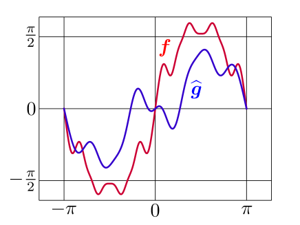
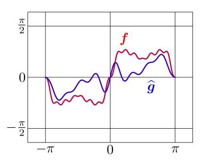
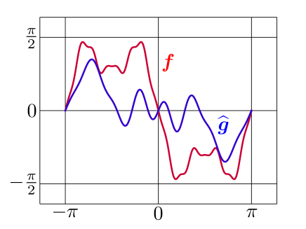
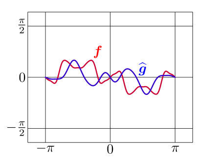
The trials used uniformly distributed pseudo-random numbers on generated in Matlab. The results of trials , , and show a typical range of outcomes. The corresponding pseudo-random numbers were
In this example it is easy to check that
and hence there is no estimation error. We can explain this by noting that contains complete information about the outcome and that we have used known theoretical information to construct the key matrices and . In addition there are no observation errors in our model. In practice may not contain complete information about the outcome, the observed values of will normally contain measurement errors, and the key matrices will likely be estimated from experimental data obtained under laboratory conditions where both and can be observed.
12 Conclusions and future research
We have shown that the optimal least squares linear filter can be extended to estimation of random functions with values in infinite-dimensional Hilbert spaces. In particular we have shown that in those instances where the generalized inverse auto-covariance is an unbounded linear operator it is nevertheless closed and densely defined. Our future research will consider applications to signal processing and possible applications to the inversion of linear operator pencils where the resolvent operator has an isolated essential singularity at the origin [2]. These operators may arise in input retrieval problems for infinite-dimensional linear control systems [4, Section 8.4.1, pp 261–262] or in the solution of infinite systems of ordinary differential equations [1, Section 8].
References
- [1] Amie Albrecht, Phil Howlett, Geetika Verma, “The fundamental equations for the generalized resolvent of an elementary pencil in a unital Banach algebra", Linear Algebra and its Applications, 574, 2019, 216–251. https://doi.org/10.1016/j.laa.2019.03.032.
- [2] Amie Albrecht, Phil Howlett, Geetika Verma, “Inversion of operator pencils on Banach space using Jordan chains when the generalized resolvent has an isolated essential singularity", Linear Algebra and its Applications, 595, 2020, 33–62. https://doi.org/10 1016/j.laa.2020.02.030.
- [3] M Ash, “Neither a Worst Convergent Series nor a Best Divergent Series Exists", The College Mathematics Journal, 28, 4, 1997, 296–297. https://doi.org/10.1080/07468342.1997.11973879.
- [4] Konstantin E. Avrachenkov, Jerzy A. Filar, Phil G. Howlett, Analytic Perturbation Theory and Its Applications, SIAM, Philadelphia, 2013, OT 135.
- [5] A V Balakrishnan, Applied functional analysis, Applications of Mathematics 3, Springer, New York, 1976.
- [6] S.L. Cotter, M. Dashti, J.C. Robinson and A.M. Stuart, “Bayesian inverse problems for functions and applications to fluid mechanics", Inverse Problems, 25, 2009, 115008. doi: 10.1088/0266-5611/25/11/115008.
- [7] N Dunford and J T Schwartz, Linear operators, Part1, General theory, Wiley, NewYork, 1988.
- [8] Heinz W Engl and M Z Nashed, “New Extremal Characterizations of Generalized Inverses of Linear Operators", Journal of Mathematical Analysis and Applications, 82, 1981, 566–586. https://doi.org/10.1016/0022-247X(81)90217-1.
- [9] Vladimir N Fomin and Michael V Ruzhansky, “Abstract optimal linear filtering", SIAM Journal on Control and Optimization, 38, 5, 2000, 1334–1352. https://doi.org/10.1137/S036301299834778X.
- [10] P R Halmos, Measure theory, University Series in Higher Mathematics, 12th printing Van Nostrand, Princeton, 1968.
- [11] Simon Haykin, Adaptive Filter Theory, International Edition, 5th Edition, Pearson Higher Ed USA, 2013.
- [12] P.G. Howlett, “Input retrieval in finite dimensional linear systems", ANZIAM J. (formerly J. Austral. Math. Soc. Ser. B) 23, 1982, 357–382. https://doi.org/10.1017/S033427000000031X.
- [13] P G Howlett, C E M Pearce and A P Torokhti, “An optimal linear filter for random signals with realisations in a separable Hilbert space", ANZIAM J, 44, 2003, 485–500. https://doi.org/10.1017/S1446181100012888.
- [14] Y Hua and W Q Liu, “Generalized Karhunen-Loeve transform", IEEE Signal Process. Lett., 5, 1998, 141–142. https://doi.org/10.1109/97.681430.
- [15] M Z Nashed, “Inner, outer and generalized inverses in Banach and Hilbert spaces", Numerical Functional Analysis and Optimization, 9, (3-4), 1987, 261–325. https://doi.org/10.1080/01630568708816235.
- [16] A W Naylor and G R Sell, Linear Operator Theory in Engineering and Science, Applied Mathematical Sciences 40, Springer-Verlag, New York, 1982.
- [17] H W Sorenson, Parameter estimation, principles and problems, Marcel Dekker, New York, 1980.
- [18] Y Yamashita and H Ogawa, “Relative Karhunen-Loeve transform", IEEE Trans. Signal Process., 44, 1996, 371–378. https://doi.org/10.1109/78.485932.
- [19] Kôsaku Yosida, Functional Analysis, Fifth Edition, Classics in Mathematics, Springer-Verlag, New York, 1978.