One Shot 3D Photography

Abstract.

3D photography is a new medium that allows viewers to more fully experience a captured moment. In this work, we refer to a 3D photo as one that displays parallax induced by moving the viewpoint (as opposed to a stereo pair with a fixed viewpoint). 3D photos are static in time, like traditional photos, but are displayed with interactive parallax on mobile or desktop screens, as well as on Virtual Reality devices, where viewing it also includes stereo. We present an end-to-end system for creating and viewing 3D photos, and the algorithmic and design choices therein. Our 3D photos are captured in a single shot and processed directly on a mobile device. The method starts by estimating depth from the 2D input image using a new monocular depth estimation network that is optimized for mobile devices. It performs competitively to the state-of-the-art, but has lower latency and peak memory consumption and uses an order of magnitude fewer parameters. The resulting depth is lifted to a layered depth image, and new geometry is synthesized in parallax regions. We synthesize color texture and structures in the parallax regions as well, using an inpainting network, also optimized for mobile devices, on the LDI directly. Finally, we convert the result into a mesh-based representation that can be efficiently transmitted and rendered even on low-end devices and over poor network connections. Altogether, the processing takes just a few seconds on a mobile device, and the result can be instantly viewed and shared. We perform extensive quantitative evaluation to validate our system and compare its new components against the current state-of-the-art.

(a) Input

$\underbracket{\parbox[t]{78.7743pt}{\vspace{0mm}\centering\leavevmode\hbox{\set@color\vspace{0mm}\centering\vspace{0mm}\centering\includegraphics[height=105.2751pt]{figures/teaser/depth.png}\@add@centering\@add@centering}\\ \vspace{\capgap}\small(b) Depth estimation\\ \footnotesize(230 ms)\@add@centering}\hskip 2.84526pt\parbox[t]{44.0847pt}{\vspace{0mm}\centering\leavevmode\hbox{\set@color\vspace{0mm}\centering\vspace{0mm}\framebox{\includegraphics[height=105.2751pt,trim=150.5625pt 0.0pt 250.93748pt 0.0pt,clip]{figures/teaser/ldi_depth.png}}\@add@centering}\\ \vspace{\capgap}\small(c) Layer generation\\ \footnotesize(94 ms)\@add@centering}\hskip 2.84526pt\parbox[t]{44.0847pt}{\vspace{0mm}\centering\leavevmode\hbox{\set@color\vspace{0mm}\centering\vspace{0mm}\framebox{\includegraphics[height=105.2751pt,trim=150.5625pt 0.0pt 250.93748pt 0.0pt,clip]{figures/teaser/ldi_inpainted.png}}\@add@centering}\\ \vspace{\capgap}\small(d) Color inpainting\\ \footnotesize(540 ms)\@add@centering}\hskip 2.84526pt\parbox[t]{86.0013pt}{\vspace{0mm}\centering\leavevmode\hbox{\set@color\vspace{0mm}\centering\vspace{0mm}\includegraphics[height=105.2751pt]{figures/teaser/mesh.png}\@add@centering}\\ \vspace{\capgap}\small(e) Meshing\\ \footnotesize(234 ms)\@add@centering}}_{\begin{subarray}{c}\vspace{-3.0mm}\\ \hbox{\pagecolor{white}~{}~{}Processing: 1,098ms on a mobile phone (iPhone 11 Pro)~{}~{}}\end{subarray}}$ (f) Novel view
(real-time)

Figure 1. We present a system for creating 3D photos from a single mobile phone picture (a). The process involves learning-based algorithms for estimating depth from the 2D input (b) and texture inpainting (d), as well as conventional algorithms for lifting the geometry to 3D and extending it in parallax regions (c), as well as generating a final mesh-based representation (e). All steps are optimized to be fast given the limited compute and memory resources available on a mobile device. The resulting representation (f) can be viewed instantly, generating novel viewpoints at real-time rates.

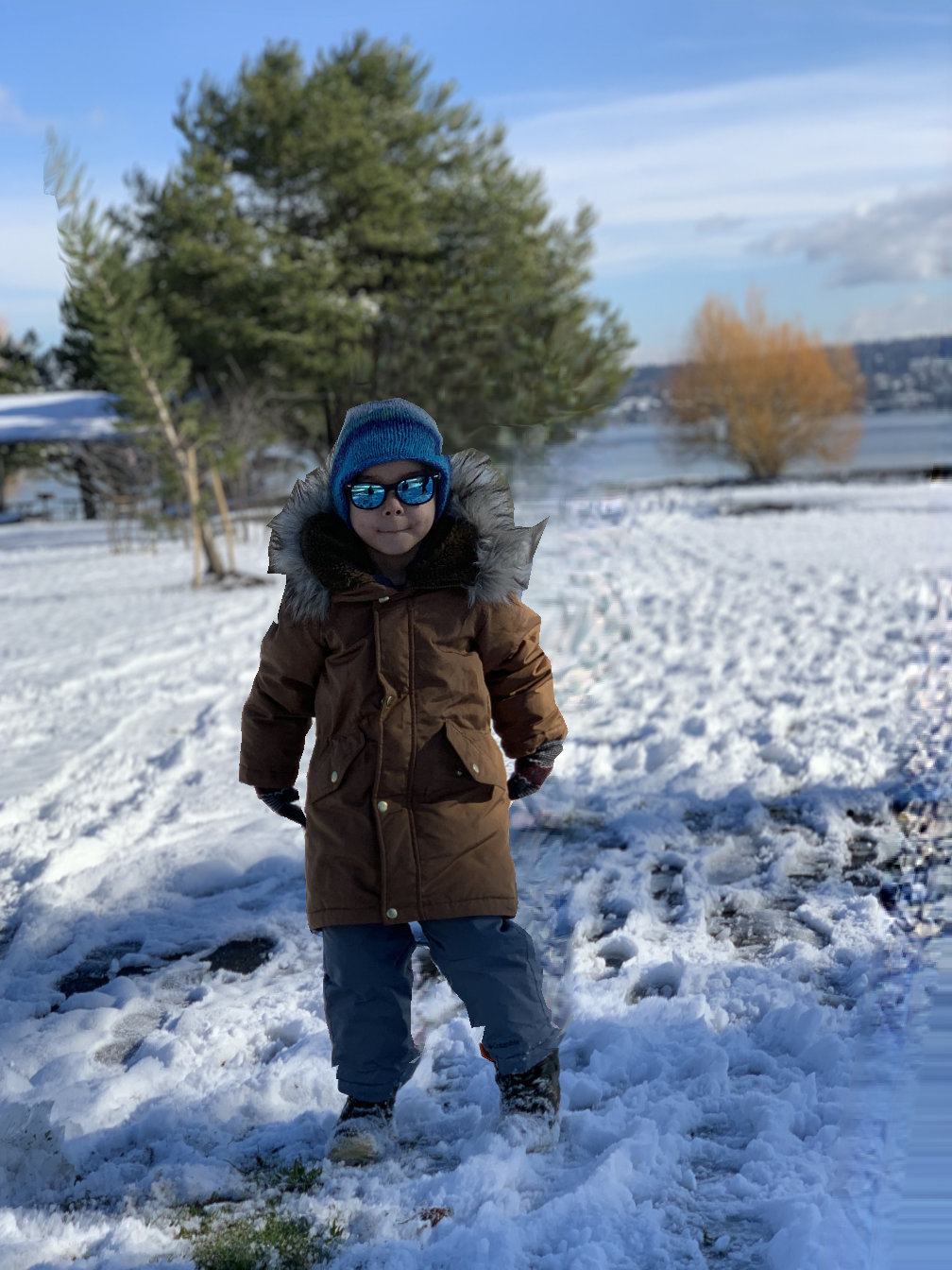
[We present a system for creating 3D photos from single-shot cell phone pictures.] We present a system for creating 3D photos from a single mobile phone picture (a). The process involves learning-based algorithms for estimating depth from the 2D input (b) and texture inpainting (d), as well as conventional algorithms for lifting the geometry to 3D and extending it in parallax regions (c), as well as generating a final mesh-based representation (e). All steps are optimized to be fast given the limited compute and memory resources available on a mobile device. The resulting representation (f) can be viewed instantly, generating novel viewpoints at real-time rates.

1. Introduction

Traditional 2D photography lets us capture the world around us, with a single click, as an instant frozen in time. 3D photography is a new way to make these captured moments come back alive. We use the term 3D photo to refer to any representation that can be displayed with parallax induced by viewpoint motion at viewing time (as opposed to a stereo pair, where inter-ocular parallax is baked in at capture time). Although still static in time, 3D photos can be interactively explored. The ability to change the viewpoint is compelling on “flat” mobile or desktop screens, and enables truly life-like experiences in Virtual Reality, by adding stereo viewing to head-motion induced parallax.

However, creating and displaying 3D photos poses challenges that are not present in 2D or even stereo photography: dense depth is required in addition to color, viewpoint changes reveal previously occluded parts of the scene that must be filled, and the affordances for changing the viewpoint must be developed.

Accurately triangulating depth requires capturing at least two views of the scene; reconstructing occluded content requires even more captured views (Hedman et al., 2017; Zitnick et al., 2004). This goes beyond the effort that most people are willing to spend on a photograph. While some high-end smartphones are equipped with multi-lens cameras that can be used to estimate depth from stereo, they do not help with occluded regions, due to the small baseline of the lenses. More importantly, there is currently at least an order of magnitude more phones in use that only have regular single-lens cameras.

We propose a system that provides a more practical approach to 3D photography. Specifically, we address these design objectives:

Effort::

the capture should occur in a single shot and not require any special hardware.

Accessibility::

creation should be accessible on any mobile device, even devices with regular, single-lens cameras.

Speed::

all post-capture processing should at most take a few seconds (on the mobile device) before the 3D photo can be viewed and shared.

Compactness::

the final representation should be easy to transmit and display on low-end devices for sharing over the internet.

Quality::

rendered novel views should look realistic; in particular, depth discontinuities and disocclusions should be handled gracefully.

Intuitive Interaction::

interacting with a 3D photo must be in real-time, and the navigation affordances intuitive.

Our system relies only on a single image as input, and estimates the depth of the scene as well as the content of parallax regions using learning-based methods. It comprises four algorithm stages (Figure 1b–e), each containing new technical contributions:

Depth Estimation::

A dense depth map is estimated from the input image using a new neural network, constructed with efficient building blocks and optimized with automatic architecture search and int8-quantization for fast inference on mobile devices. It performs competitively w.r.t. the state-of-the-art while consuming considerably fewer resources and having fewer parameters.

Layer Generation::

The pixels are lifted onto a layered depth image (LDI), and we synthesize new geometry in parallax regions using carefully designed heuristic algorithms.

Color Inpainting::

We synthesize colors for the newly synthesized geometry of the LDI using an inpainting neural network. A novel set of neural modules enables us to transform this 2D CNN to one that can be applied to the LDI structure directly.

Meshing::

Finally, we create a compact representation that can be efficiently rendered even on low-end devices and effectively transferred over poor network connections.

All processing steps are optimized for running fast on a mobile device with limited available resources. We also discuss affordences for viewing 3D photos on mobile and fixed flat screens, as well as using head-mounted displays for virtual reality.

We validate our system through extensive quantitative evaluation of our system’s components, in particular, comparing depth estimation and inpainting to alternative state-or-the-art algorithms. We believe that our proposed system, altogether, largely achieves the stated objectives and makes 3D photography truly practical and accessible for everyone.

2. Previous Work

Manual annotation:

The classic way to create 3D images, proposed in the seminal “tours into the picture” (Horry et al., 1997), involves carefully annotating the depth of a picture manually. This can also be done semi-manually with the help of tools (Oh et al., 2001). While the manual-assisted approach promises the ability to generate arbitrarily high quality depth maps for downstream processing, depth annotation is a laborious process and requires a skilled user.

Single-image depth estimation:

Since the seminal paper of Saxena et al. (2006) there has been considerable progress on estimating depth from a single image, by leveraging advances in deep learning. Chen et al. (2016) propose a convolutional neural network (CNN) architecture and large quantities of training photos with ordinally labeled point pairs, and provide substantially improved generalization capability compared to previous work. Li and Snavely (2018) provide even denser depth annotation from large-scale photometric reconstruction. Networks can also be trained with a photometric loss and stereo supervision (Garg et al., 2016; Godard et al., 2017; Kuznietsov et al., 2017; Godard et al., 2019), which might be easier to obtain than depth annotation. In addition, synthetic data (Ramamonjisoa and Lepetit, 2019; Niklaus et al., 2019) might help with synthesizing sharper depth discontinuities. Ranftl et al. (2019) show a good improvement by training from several datasets. While the work mentioned above achieves commendable results, the proposed network architectures are too resource intensive in terms of processing, memory consumption and model size for mobile devices (Section 6.4). We propose a new architecture in this work that performs competitively, but is considerably faster and smaller.

In terms of accelerating CNNs for monocular depth inference, Wofk et al. (2019), Poggi et al. (2018), and Peluso et al. (2019) each proposed a low-latency architecture for real-time processing on embedded platforms. Lin et al. (2020) explored reducing the memory footprint of monocular depth estimation networks by super-resolving predicted depth maps. Finally, Tonioni et al. (2019) proposed an online domain adaptation learning technique suitable for realtime stereo inference. We compare against some of these methods in Section 6.4.

Layered Depth Images:

Shade et al. (1998) provide a taxonomy of representations for 3D rendering and our work leverages one of them for processing. In particular, we leverage Layered Depth Images (LDI), similar to recent work (Hedman et al., 2017; Hedman and Kopf, 2018), but with more sophisticated heuristics for inpainting occlusions, and optimized algorithms to compute the result within seconds on mobile devices. LDI provide an easy-to-use representation for background expansion and inpainting, and lend themselves for conversion into a textured triangle mesh for final content delivery and rendering.

Multi-plane Images:

Stereo Magnification (Zhou et al., 2018) proposed synthesizing a Multi-plane Image (MPI) representation, i.e., a stack of fronto-parallel planes with RGB$\alpha$ textures, from a small-baseline stereo pair. This work is extended to Srinivasan et al. (2019) to reduce the redundancy in the representation and expand the ability to change the viewpoint. Flynn et al. (2019) generate high-quality MPIs from a handful of input views using learned gradient descent, and Mildenhall et al. (2019) blend a stack of MPIs at runtime. All MPI generation methods above have in common that they require two or more views as input, while our proposed method uses only a single input image.

Other Representations and Neural Rendering:

Sitzmann et al. (2019) encode the view-dependent appearance of a scene in a voxel grid of features and decode at runtime using a “neural renderer”. Other methods (Martin-Brualla et al., 2018; Meshry et al., 2019) also leverage on-the-fly neural rendering to increase the photorealism of their results. However, these methods do not guarantee that disocclusions are filled consistently from different viewing angles, and they require too powerful hardware at runtime to perform in real-time on mobile devices.

Single-image Novel View Synthesis:

Most aforementioned view synthesis methods require multiple input images, while there are only a few that can operate with a single input image, like ours. This is important to mention, because view synthesis from a single input image is a considerably more difficult and ill-posed problem. Yet, it is desirable, because requiring a user to capture a single view is more practical and the method can even be applied retro-actively to any existing photo, as demonstrated with historical photos in the accompanying video.

Liu et al. (2018a) predict a set of homography warps, and a selection map to combine the candidate images to a novel view. It employs complex networks at runtime, leading to slow synthesis. Srinivasan et al. (2017) predict a 4D light field representation. This work has only been demonstrated in the context of narrow datasets (e.g., of plants, toys) and has not been shown to generalize to more diverse sets.

3. Overview

3D photography requires a geometric representation of the scene. There are many popular choices, although some have disadvantages for our application. Light fields capture very realistic scene appearance, but have excessive storage, memory, and processing requirements. Meshes and voxels are very general representations, but are not optimized for being viewed from a particular viewpoint. Multi-plane images are not storage and memory efficient, and exhibit artifacts for sloped surfaces at large extrapolations.

In this paper we build on the Layered Depth Image (LDI) representation (Shade et al., 1998), as in previous work (Hedman et al., 2017; Hedman and Kopf, 2018). An LDI consists of a regular rectangular lattice with integer coordinates, just like a normal image; but every position can hold zero, one, or more pixels. Every LDI-pixel stores a color and a depth value. Similar to Zitnick et al. (2004), we explicitly represent the 4-connectivity of pixels between and among layers, i.e., every pixel can have either zero or exactly one neighbor in each of the cardinal directions (left, right, up, down).

This representation has significant advantages:

Sparsity::

It only stores features that are present in the scene.

Topology::

LDIs are locally like images. Many fast image processing algorithms translate to LDIs.

Level-of-detail::

The regular sampling in image-space provides inherent level-of-detail: near geometry is more densely sampled than far geometry.

Meshing::

LDIs can be efficiently converted into textured meshes (Sections 4.4.1-4.4), which can be efficiently transmitted and rendered.

While LDIs have been used before to represent captured scenes (Hedman et al., 2017; Hedman and Kopf, 2018), our work makes several important contributions: (1) unlike previous work, our algorithm is not limited to only producing at most two layers at any point; (2) we better shape the continuation of depth discontinuities into the disoccluded region using constraints; (3) we propose a new network for inpainting occluded LDI pixels, as well as a method to translate existing 2D inpainting networks to operate directly on LDIs; (4) efficient algorithms for creating texture atlases and simplified triangle meshes; (5) our complete algorithm is faster and runs end-to-end in just a few seconds on a mobile device.

In the next section, we describe our algorithm for creating 3D photos from single color images. Next, we describe in Section 5 how they are experienced on mobile and fixed flat screens, as well as using head-mounted displays for virtual reality. Finally, in Section 6 we provide detailed quantitative evaluation of our algorithm components as well as comparisons to other state-of-the-art methods.

4. Creating 3D Photos

The input to our method is a single color image. It is typically captured with a mobile phone, but any other photo may be used (e.g., historical pictures).

Our system comprises four stages (Figure 1b–e) and runs end-to-end on the mobile capture device. We describe depth estimation in Section 4.1, lifting to an LDI and synthesizing occluded geometry in Section 4.2, inpainting color on the occluded layers in Section 4.3, and converting the LDI into the final mesh representation in Section 4.4.

4.1. Depth Estimation

Figure 2. Depth estimation network schematic. Gray TR blocks are used in down-/up-sampling passes and blue TR blocks are used to preserve spatial resolution. TR Blocks are defined in Fig. 3. Mona Lisa, by Leonardo da Vinci (public domain).

The first step in our algorithm is to estimate a dense depth map from the input image. Monocular depth estimation is a very active field, and many competitive methods have just appeared in the months prior to writing (Ranftl et al., 2019; Ramamonjisoa and Lepetit, 2019; Niklaus et al., 2019; Godard et al., 2019). While these methods achieve high quality results, they use large models that consume considerable resources during inference. This makes it difficult to deploy them in a mobile application. In fact, most of these methods cannot run even on high-end smart phones due to the limited memory on these platforms (see Section 6.4).

In this section we propose a new architecture, called Tiefenrausch, that is optimized to consume considerably fewer resources, as measured in terms of inference latency, peak memory consumption, and model size, while still performing competitively to the state-of-the-art.

These improvements were achieved by combining three techniques: (1) building an efficient block structure that is fast on mobile devices, (2) using a neural architecture search algorithm to find a network design that achieves a more favorable trade-off between accuracy, latency, and model size, and, then, (3) using 8-bit quantization to achieve a further reduction of the model size and latency while retaining most of the accuracy. Below, we describe these optimizations as well as the training procedure in detail.

Efficient Block Structure

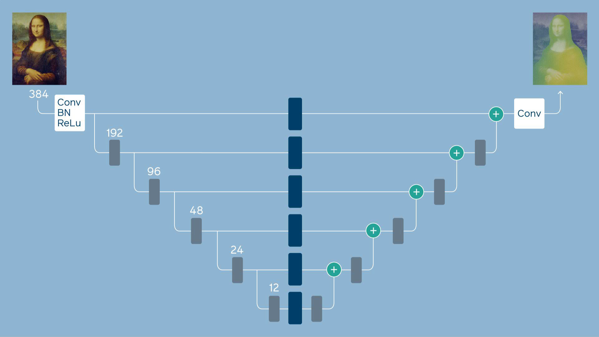
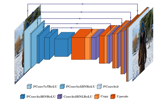
We built an efficient block structure inspired by previous work (Sandler et al., 2018; Wu et al., 2019) and is illustrated in Fig.  3. The block contains a sequence of point-wise (1x1) convolution, KxK depthwise convolution where K is the kernel size, and another point-wise convolution. Channel expansion, $e$, is a multiplicative factor which increases the number of channels after the initial point-wise convolution. In layers which decrease the spatial resolution, depthwise convolution with stride, $s_{d}>1$, is used. When increasing the spatial resolution, we use nearest neighbor interpolation with a scale factor, $s_{u}>1$, after the initial point-wise convolution. If the output dimensions of the block are the same as the input dimensions (i.e., $s_{d}=s_{u}=1$, $C_{in}=C_{out}$), then a skip connection is added between the input and output with an additional block in the middle.

We combine these blocks into a U-Net like architecture (Chen et al., 2016; Li and Snavely, 2018; Ronneberger et al., 2015) as shown in Fig.  2. We fixed the number of downsampling stages to 5 where each stage has a downsampling factor $s_{d}=2$. All stages have 3 blocks per stage and skip connections are placed between stages with the same spatial resolution.

Figure 3. Block structure used to create the depth estimation architecture.  $s_{u}$ and $s_{d}$ refer to the up and down sampling scale factors, respectively, and $e$ is the channel expansion factor. Refer to the text for details.

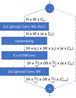
[Block structure used to create the depth estimation architecture.]Block structure used to create the depth estimation architecture.

Neural Architecture Search

We then use the Chameleon methodology (Dai et al., 2019) to find an optimal design given an architecture search space. Briefly, the Chameleon algorithm iteratively samples points from the search space to train an accuracy predictor. This accuracy predictor is used to accelerate a genetic search to find a model that maximizes predicted accuracy while satisfying specified resource constraints. In this setting, we used a search space which varies the channel expansion factor and number of output channels per block resulting in $3.4\times 10^{22}$ possible architectures. We set a FLOP constraint on the model architecture and can vary this constraint in order to achieve different operating points. The total time to search was approximately three days using 800 Tesla V100 GPUs.

Quantization

The result of the architecture search is an optimized model with a reduced FLOP count and a lower number of parameters. As our model is friendly for low-bit precision computation, we further improve the model by quantizing the 32-bit floating point parameters and activations (Choi et al., 2018) to 8-bit integers. This achieves a $4\times$ model size reduction as well as a reduction in inference latency and has been shown to result in only a small accuracy loss in other tasks (Dai et al., 2019). We use a standard linear quantizer on both the model parameters and the activations. Furthermore, we utilize Quantization-Aware Training (QAT) in order to determine the quantization parameters (Jacob et al., 2018) so that performance translates between training and inference. Our architecture is particularly amenable to quantization and QAT, because it only contains standard 1x1 convolution, depth-wise convolution, BatchNorm, ReLU and resize operations and both convolutions are memory-bounded. The model can be further simplified by fusing BatchNorm operations with convolutions and ReLU can be handled by fixing the lower bound of the quantization parameters to zero. The convolution and resize operators are the only operators retained in the final model.

Training Details

We train the network with the MegaDepth dataset, and the scale-invariant data loss and the multi-scale scale-invariant gradient loss proposed by Li and Snavely  (2018), but exclude the ordinal loss term. The training runs for 100 epochs using minibatches of size 32 and the Adam optimizer with $\beta_{1}=0.5$ and $\beta_{2}=0.999$. The ground truth depth maps in the MegaDepth dataset do not include depth measurements for the sky region. We found that using this data as-is led to a network that would not reliably place the sky in the background. To overcome this limitation we leverage PSPNet (Zhao et al., 2017) to identify the sky region in the images. We then replace any missing depth information in the sky region with twice the maximal depth observed in the depth map. Intuitively, this forces the sky to have the largest depth in the scene for all MegaDepth images.

To prevent overfitting to specific camera characteristics in our data we perform data augmentation by varying color saturation, contrast, image brightness, hue, image area, field of view, and left-right flipping. Specifically, all images have an aspect ratio of 4:3 (or its inverse) and are first uniformly resized so the short side is $288\alpha$ pixels long. $\alpha$ is a uniform random sample in $\left[1,1.5\right]$ to avoid overfitting to the field of view of the training data. The resize operation uses nearest neighbor point sampling for both the depth map and the image (it, interestingly, performed better than proper anti-aliased sampling). Next, we select a random crop of size $(288,288)$ from the resized image and depth map. Finally, we apply random horizontal flipping to the $(288,288)$ image and depth map crops.

Another deficiency we found with early networks was that they failed to generalize to images from lower quality cameras. The images in the MegaDepth dataset are well-exposed, but we often found that other cameras fail to provide such good exposure. To enable robustness to image color variations, we combine the above data augmentation with the following color data augmentation. We vary the brightness of the image by a gamma adjustment with a uniformly distributed factor in $[0.6,1.4]$. Similarly, we vary the contrast uniformly between 60% and 100% (i.e., blending with a middle-gray image) as well as the color saturation of the image. Finally, images are converted to the HSV colorspace and the hue is rotated by a uniformly distributed value in $[-25^{\circ},25^{\circ}]$ before being converted back to RGB.

4.2. Lifting to Layered Depth Image

(a) Raw / cleaned depth image

(b) Raw

(c) Filtered

(d) Cleaned

Figure 4. Depth image before and after cleaning (a). Discontinuities are initially smoothed out over multiple pixels. Weighted median filter sharpens them successfully in most places (c). We fix remaining isolated features at middle-values using connected component analysis (d).

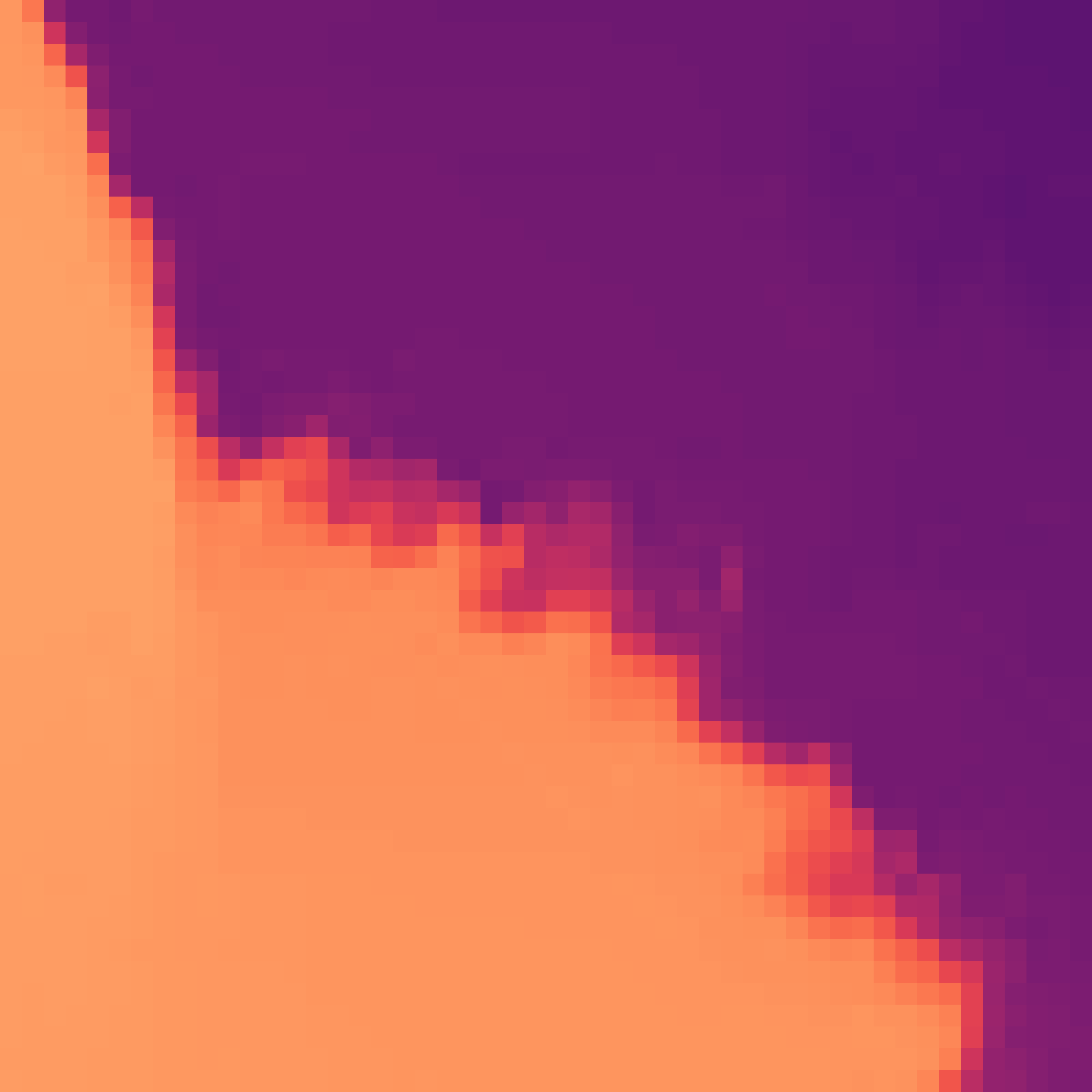
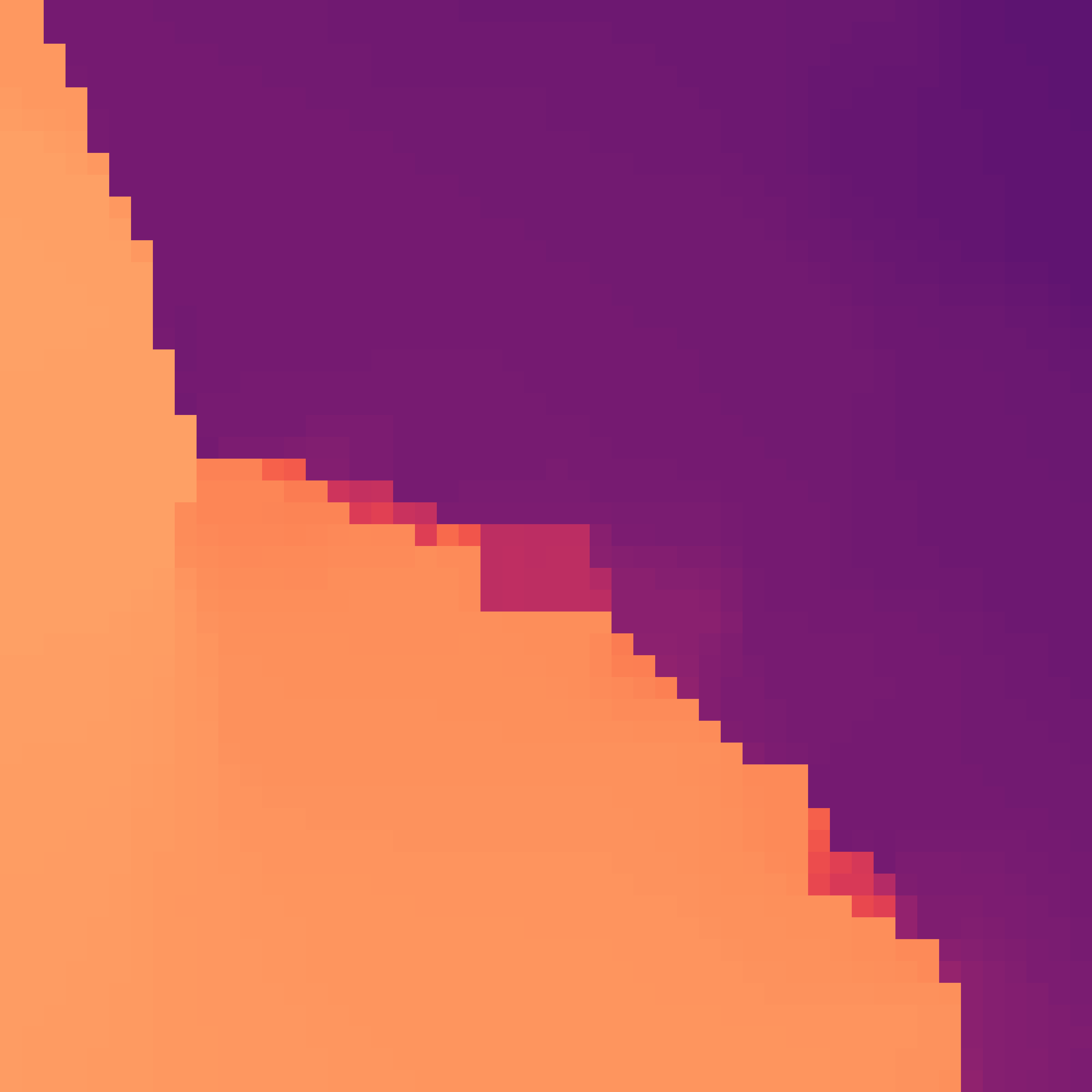
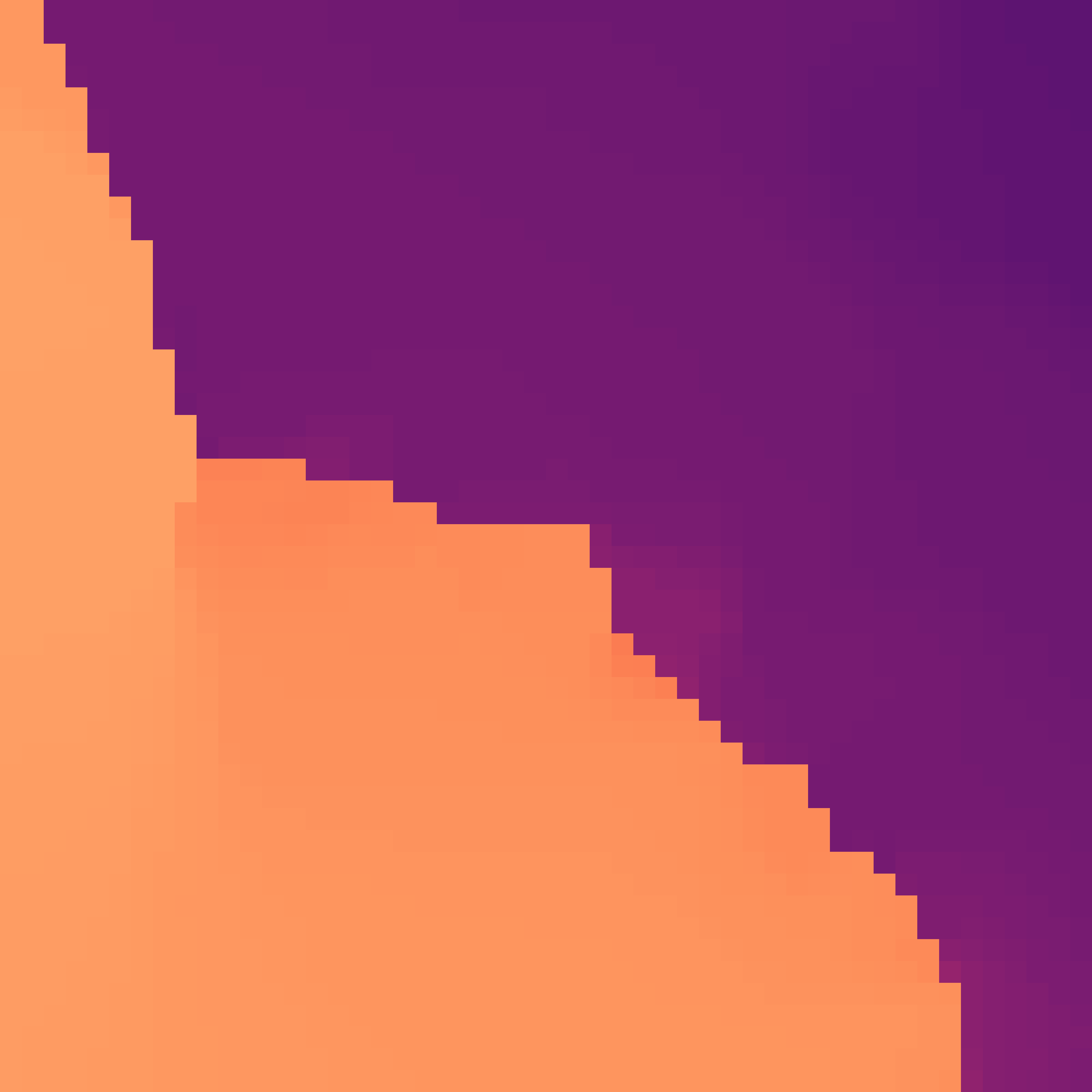
[Depth image before and after cleaning.] Depth image before and after cleaning (a). Discontinuities are initially smoothed out over multiple pixels. Weighted median filter sharpens them successfully in most places (c). We fix remaining isolated features at middle-values using connected component analysis (d).

Now that we have obtained a dense depth map, we are ready to lift the image to the LDI representation. This will allow us to express multiple layers, so we can show detail in parallax regions. These are details that have not been observed in the input view, they have to be synthesized.

After discussing depth pre-processing in Section 4.2.1, we will discuss hallucinating new geometry in parallax regions in Section 4.2.2, and finally inpainting of color on the new geometry in Section 4.3.

4.2.1. Depth Pre-processing

The most salient geometric feature in 3D photos are depth discontinuities. At those locations we need to extend and hallucinate new geometry behind the first visible surface (as will be explained in the next section). The depth images obtained in the previous section are typically over-smoothed due to the regularization inherent to the machine learning algorithms that produced them. This smoothing “washes out” depth discontinuities over multiple pixels and often exhibit spurious features that would be difficult to represent (Figure 4b). The goal of the first algorithm stage is to de-clutter depth discontinuities and sharpen them into precise step edges.

We first apply a weighted median filter with a $5\times 5$ kernel size. Depth values within the kernel are Gaussian-weighted by their disparity difference to the center pixel (using $\sigma_{\textit{\!disparity}}=0.2$). The weighting of the filter is important to preserve the localization of discontinuities, and, for example, avoid rounding off corners. Since we are interested in forcing a decision between foreground and background, we disable the weights of pixels near the edge (i.e., pixels that have a neighbor with more than $\tau_{\textit{disp}}=0.05$ disparity difference.)

This algorithm succeeds in sharpening the discontinuities. However, it occasionally produces isolated features at middle-depth values (Figure 4c). We perform a connected component analysis (with threshold $\tau_{\textit{disp}}$) and merge small components with fewer than 20 pixels into either foreground or background, whichever has a larger contact surface (Figures 4d).

4.2.2. Occluded Surface Hallucination

(a) Expansion constraints

(b) Instant3D N-layer

(c) Instant3D 2-layer

(d) Our method

Figure 5. Expanding geometry on the back-side of discontinuities into occluded parts of the scene. Previous work (Hedman and Kopf, 2018) produces artifacts at T-junctions: either extraneous geometry if left unconstrained (b) or cracked surfaces when using their suggested fix (c). We improve this by grouping discontinuities into curve-like features (color-coded), and inferring spatial constraints to better shape their growth (dashed lines).

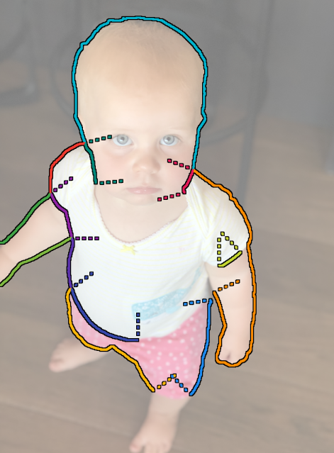
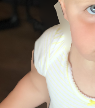
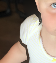
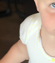
[Expanding geometry on the back-side of discontinuities into occluded parts of the scene.] Expanding geometry on the back-side of discontinuities into occluded parts of the scene. Previous work (Hedman and Kopf, 2018) produces artifacts at T-junctions: either extraneous geometry if left unconstrained (b) or cracked surfaces when using their suggested fix (c). We improve this by grouping discontinuities into curve-like features (color-coded), and inferring spatial constraints to better shape their growth (dashed lines).

 

(a) Pixel labels

 

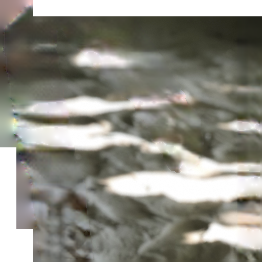
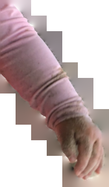
(b) Inpainted and padded

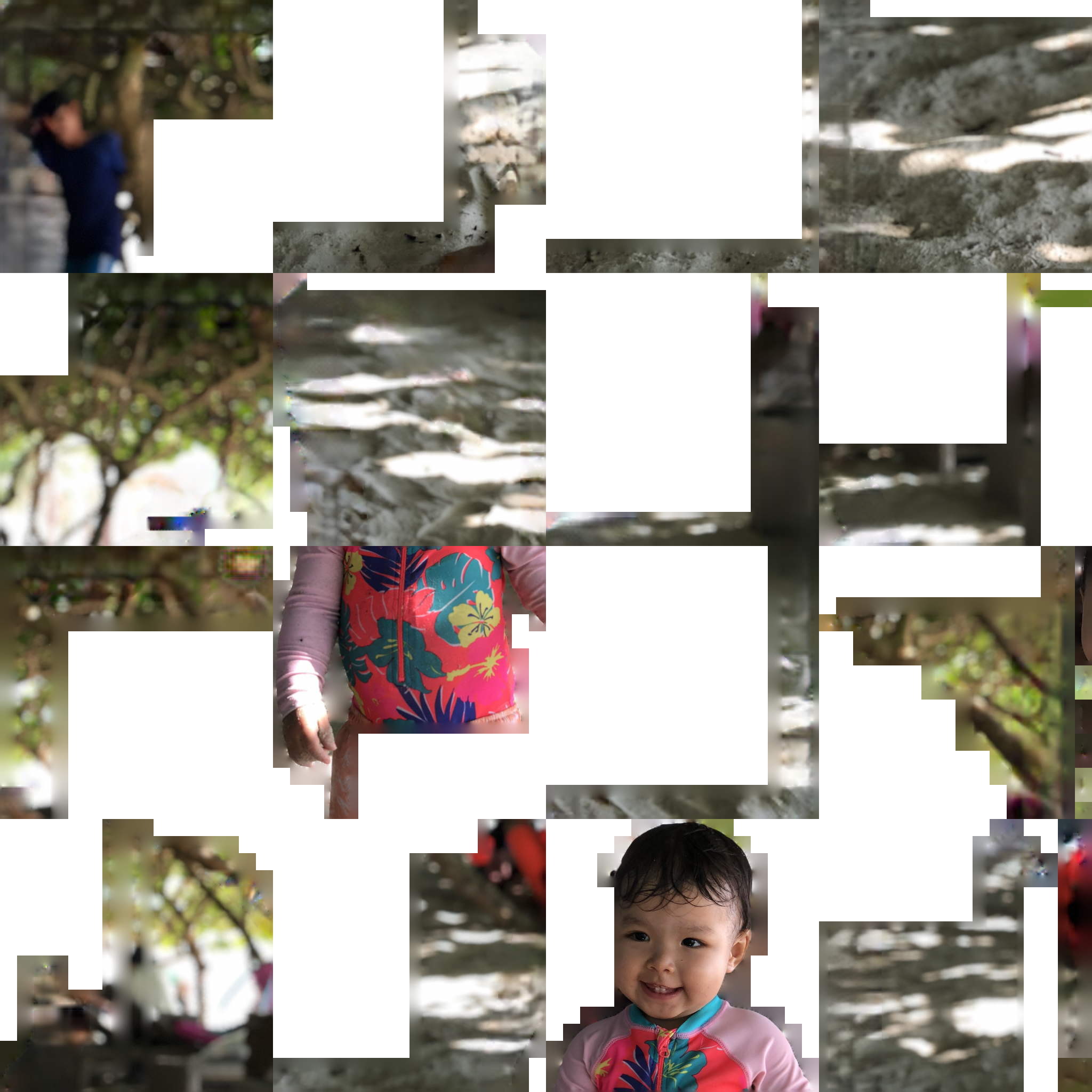
(c) Packed texture atlas

Figure 6. Partitioning the layered depth image into charts for texturing. (a) Pseudo-coloring different kinds of pixels that require inpainting, on two example charts. Dark blue pixels are occluded, and light blue pixels are on the foreground but close to a discontinuity, and, therefore, contain possibly mixed colors. Red pixels add padding for texture filtering: dark red pixels (at silhouettes) are inpainted and light red pixels (elsewhere) are copied from adjacent charts. Green pixels add padding for JPEG macroblocks (see text). (b) Final inpainted charts. (c) Packed atlas.

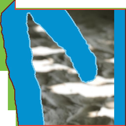
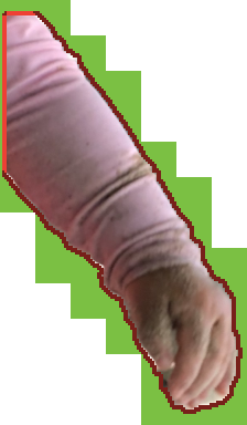
[Partitioning the layered depth image into charts for texturing.] Partitioning the layered depth image into charts for texturing. (a) Pseudo-coloring different kinds of pixels that require inpainting, on two example charts. Dark blue pixels are occluded, and light blue pixels are on the foreground but close to a discontinuity, and, therefore, contain possibly mixed colors. Red pixels add padding for texture filtering: dark red pixels (at silhouettes) are inpainted and light red pixels (elsewhere) are copied from adjacent charts. Green pixels add padding for JPEG macroblocks (see text). (b) Final inpainted charts. (c) Packed atlas.

The goal of this stage is to “hallucinate” new geometry in occluded parts of the scene. We start by lifting the depth image onto an LDI to represent multiple layers of the scene. Initially, the LDI has a single layer everywhere and all pixels are fully connected to their neighbors, except across discontinuities with a disparity difference of more than $\tau_{\textit{disp}}$.

To create geometry representing occluded surfaces, we next extend the geometry on the backside of discontinuities iteratively behind the front-side by creating new LDI pixels. A similar algorithm has been employed by Hedman and Kopf (2018). However, their algorithm has an important limitation: pixels are allowed to extend in all directions (as long as they remain hidden behind the front layer). This causes frequent artifacts at T-junctions, i.e., where background, midground, and foreground meet: the midground grows unrestrained, expanding the foreground discontinuity and creating a cluttered result (Figure 5b). The authors reduce the undesired excess geometry by removing all but the nearest and farthest layers anywhere in the LDI. However, this creates disconnected surfaces (Figure 5c). We resolve these problems by grouping discontinuities into curve-like features and inferring spatial constraints to better shape their growth (Figure 5d). We group neighboring discontinuity pixels together, but not across junctions (see color coding in Figure 5a). At this point, we remove spurious (shorter than 20 pixels) groups from consideration.

In one extension iteration, each group grows together as one unit, creating a one pixel wide “wave front” of new LDI pixels. To avoid the previously mentioned cluttering problem, we restrain curves from growing beyond the perpendicular straight line at their end points (dotted lines in Figure 5a). 3-way intersections deserve special consideration: at these points there are 3 different depths coming together, but we are only interested in constraining the midground, while the background should be allowed to freely grow under both of the other layers. Therefore, we only keep the one of the three constraints at 3-way intersections that is associated with the mid-/foreground discontinuity (Figure 5a).

The depth of newly formed pixels is assigned an average of their neighbors, and the color is left undefined for now (to be inpainted in the next section). Intersecting groups are merged if their disparity difference is below $\tau_{\textit{disp}}$. We run this expansion algorithm for 50 iterations to obtain a multi-layered LDI with sufficient overlap for displaying it with parallax.

4.3. LDI Inpainting

At this point we have an LDI with multiple layers around depth discontinuities, but it is still missing color values in the parallax regions (i.e., the red pixel in Figure 1c). In this section, we discuss the inpainting of plausible colors, so that disocclusions when viewing the 3D photo appear seamless and realistic.

A naïve approach to filling missing regions in disocclusions would be to inpaint them in screen space, for example using a state-of-the-art network, such as Partial Conv (Liu et al., 2018b). However, this would not lead to desirable results, because (1) filling each view at runtime would be slow, (2) the independent synthesis would result in inconsistent views, and, finally, (3) the result would be continuous on both foreground and background sides of the missing region (while it should only be continuous on the background side), thus leading to strong blur artifacts along the edges.

A better approach would be to inpaint on the LDI structure. Then, the inpainting could be performed once, each view would be consistent by design, and, since the LDI is explicitly aware of the connectivity of each pixel, the synthesis would be only continuous across truly connected features. However, one complication is that a LDI does not lend itself easily to processing with a neural network, due to the irregular connectivity structure. One approach would be, again, to turn to filling projected views and warp the result back onto the LDI. But this might require multiple iterations from different angles until all missing pixels are covered.

Our solution to this problem uses the insight that the LDI is locally structured like a regular image, i.e., LDI pixels are 4-connected in cardinal directions. By traversing these connections we can aggregate a local neighborhood around a pixel (described below), which allows us to map network operators, such as convolutions, to the LDI. This mapping, in turn, allows us to train a network entirely in 2D and then use the pretrained weights for LDI inpainting, without having done any training with LDIs.

4.3.1. Mapping the PConv Network to LDI

We represent the LDI in tensor form as a tuple of a $C\times K$ float32 “value” tensor $\mathcal{P}$ and a $6\times K$ int32 “index” tensor $\mathcal{I}$, where $C$ is the number of channels, and $K$ the number of LDI pixels. The value tensor $\mathcal{P}$ stores the colors or activation maps, and the index tensor stores the pixel position $(x,y)$ position and $(\text{left},\text{right},\text{top},\text{bottom})$ neighbor indices for each LDI pixel. We also store a $1\times K$ binary “mask” tensor $\mathcal{M}$ which indicates which pixels are known and which pixels must be inpainted.

The PartialConv (Liu et al., 2018b) network uses a U-Net like architecture (Ronneberger et al., 2015). We map this architecture to LDI by replacing every PConv layer with LDIPConv layer which accepts an LDI ($\mathcal{P},\mathcal{I}$) and mask $\mathcal{M}$ instead of a $C\times H\times W$ color and $1\times H\times W$ mask image tensor. All value tensors at a level (i.e. scale $1/s$) of the U-Net share the same index tensor $\mathcal{I}_{s}$. Most operations in the network are point-wise, i.e., the input/output is a single pixel, for example ReLU or BatchNorm; these map trivially to the LDI. The only non-trivial operations, which aggregate kernels, are 2D convolution (the network uses $3\times 3$, $5\times 5$, $7\times 7$ kernel sizes), down-scaling (convolutions with $\text{stride}=2$), and up-scaling.

 

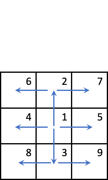
(a) 3x3 kernel

(fully connected)

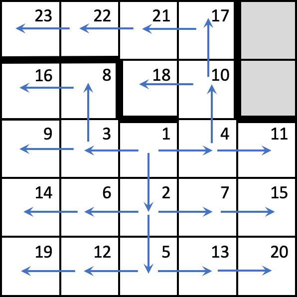
(b) 5x5 kernel

(with silhouette pixels)

Figure 7. Aggregating convolution kernels on a LDI with breadth-first exploration. The numbers indicate the traversal order. Gray elements cannot be filled and are zero-padded.

Convolution:

We aggregate the 2D convolution kernels by exploring the LDI graph in breadth-first manner: starting at the center pixel we traverse LDI pixels in up / down / left / right order to greedily fill the kernel elements. Once a kernel element has been visited we do not traverse to this position again. If an LDI pixel is unconnected in a direction (e.g., at a silhouette) we treat it as if the pixel was on an image edge i.e. zero-padding. Since we are using partial convolutions and the mask is also zero-padded, this results in partial convolution based padding (Liu et al., 2018c). For a $3\times 3$ kernel where all LDI pixels are fully connected, the pattern in Figure 7a emerges. Figure 7b shows an example of a $5\times 5$ kernel, where some silhouette pixels have no neighbors in certain directions. In this case, the breadth-first aggregation explores around these “barriers”, except for the two pixels in the top-right right that cannot be reached in any way and are partial-padded (Liu et al., 2018c).

Coarsening

Figure 8. Coarsening scheme for the up-/downscale operators.

Downscaling or Strided Convolutions:

In the image-version of the network, downscaling is done by setting a stride of 2 on convolution operations, i.e., for every $2\times 2$ block of pixels at the fine scale, only the top-left pixel is retained at the coarser scale. We implement down-scaling for the LDI in a similar way: every LDI pixel with $\operatorname{mod}\!\left(x,2\right)=\operatorname{mod}\!\left(y,2\right)=0$ is retained. If multiple LDI pixels occupy a $\left(x,y\right)$ position, they will all be retained. If for two retained pixels there was a length-2 connecting path at the fine scale, they will also be connected a the coarse scale. Figure 8 illustrates this coarsening scheme.

Upscaling:

In the image-version of the network, upscaling is done with nearest interpolation, i.e., a $2\times 2$ block of pixels at the fine scale all take the value of the corresponding 1 pixel at the coarser scale. We again, emulate this for the LDI: the whole group of LDI pixels that collapsed into a coarse pixel all take its value. We implemented the original PConv network in Caffe2 with the custom convolution and scaling operators.

4.3.2. Mobile Optimized Inpainting Network

This network enables high-quality inpainting of parallax regions on LDIs. However, similar to prior work in depth estimation, it is too large and resource intensive for mobile applications.

In the following, we propose a new architecture, called Farbrausch that is optimized in this regard. We begin with a traditional screen-space (2D) PartialConv network with 5 stages of downsampling. This network is converted to our LDI representation with our custom operators. Chameleon Search is used to identify the best set of hyperparameters encoding the number of output channels for each stage of the encoder (and similarly the paired decoder stage). In particular, FLOP count is traded off against the PartialConv inpainting loss on its validation set (Liu et al., 2018b). This hyperparameter search took 3 days on 400 V100 GPUs. In this time, 150 networks were trained to build the accuracy predictor used in the genetic search.

Figure 9. Farbrausch Network

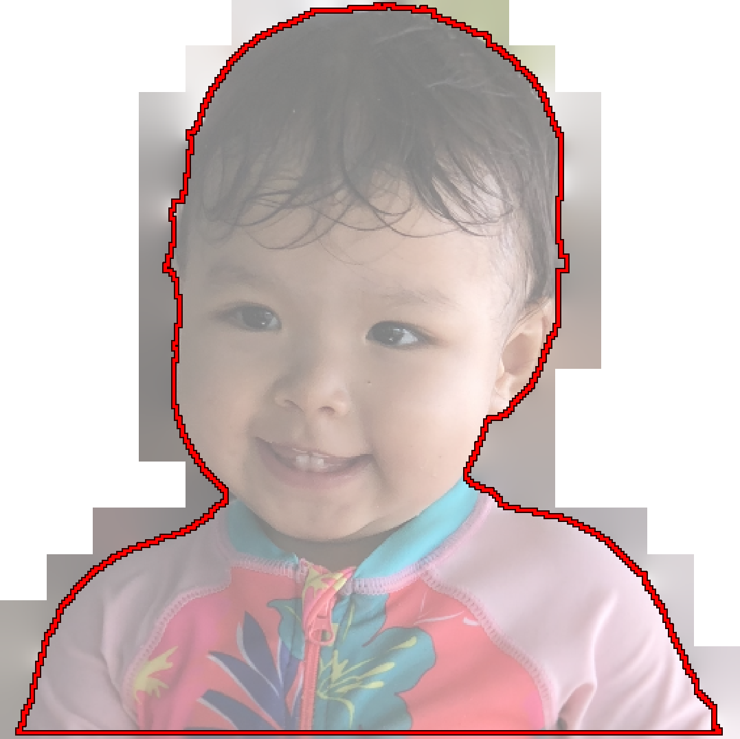
(a) Detailed polygon

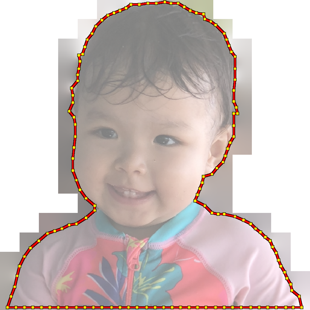
(b) Simplified polygon

(c) Interior vertices

(d) 2D triangulation

(d) Lifted to 3D

Figure 10. Directly constructing a simplified triangle mesh in the 2D atlas domain.(a) Detailed polygon from the outline of a single chart. (b) Simplified chart polygon. Adjacent charts are simplified identically to guarantee a tight fit. (c) Added interior vertices to represent depth variation and achieve more regular triangle shapes. (d) 2D triangulation. (e) Lifting the mesh to 3D by projecting vertices along their corresponding rays according to their depth.

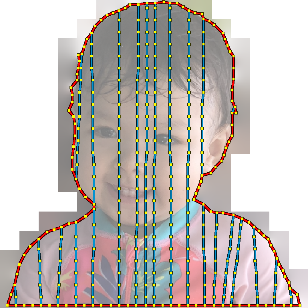
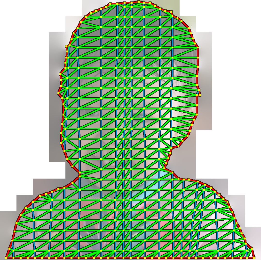
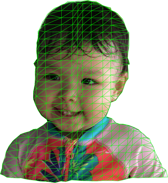
[Directly constructing a simplified triangle mesh in the 2D atlas domain.] Directly constructing a simplified triangle mesh in the 2D atlas domain.(a) Detailed polygon from the outline of a single chart. (b) Simplified chart polygon. Adjacent charts are simplified identically to guarantee a tight fit. (c) Added interior vertices to represent depth variation and achieve more regular triangle shapes. (d) 2D triangulation. (e) Lifting the mesh to 3D by projecting vertices along their corresponding rays according to their depth.

4.4. Conversion to Final Representation

Now that we have a fully inpainted multi-layer LDI, we are ready to convert it into a textured mesh, which is our final representation. This is done in two parts: creating the texture (Section 4.4.1), and the mesh generation (Section 4.4.2).

4.4.1. Texture Atlas Generation

The LDI contains many self-overlapping parts and has a complex topology. Hence, it cannot be mapped to a single contiguous texture image. We thus partition it into flat charts that can be packed into an atlas image for texturing.

Chart generation:

We use a simple seed-and-grow algorithm to create charts: the LDI is traversed in scanline order, and whenever a pixel is encountered that is not part of any chart, a new chart is seeded. We then grow the chart using a breadth-first flood fill algorithm that follows the pixel connections in the LDI, but respects several constraints:

1. charts cannot fold over in depth, since that would not be representable;

2. we cap the maximum chart size to improve packing efficiency (avoids large non-convex shapes);

3. when encountering pixels at the front side of depth edges (without neighbors in some direction), we mark a range of adjacent pixels across the edge unusable to avoid filtering operations from including pixels from different surfaces. These marked pixels will eventually land in a separate chart.

This algorithm is fast and produces charts that are reasonably efficient for packing (low count, non-complex boundaries). Figure 6 shows a few typical examples.

Texture filter padding:

When using mipmapping, filtering kernels span multiple consecutive pixels in a texture. We therefore add a few pixel thick pad around each chart. We either copy redundant pixels from neighboring charts, or use isotropic diffusion at step-edges where pixels do not have neighbors across the chart boundary (dark/light red in Figure 6, respectively).

Macroblock padding:

Another possible source of color bleeding is lossy image compression. We encode textures with JPEG for transmission, which operates on non-overlapping $16\times 16$ pixel macroblocks. To avoid bleeding we smoothly inpaint any block that is overlapped by the chart with yet another round of isotropic diffusion (green pixels in Figure 6a). Interestingly, this also reduces the encoded texture size by almost 40% compared to solid color fill, because the step edges are pushed from the chart boundaries to macroblock boundaries where they become “invisible” for the JPEG encoder.

Packing:

Finally, we pack the padded charts into a single atlas image, so the whole mesh can be rendered as a single unit. We use a simple tree-based bin packing algorithm. Figure 6c shows the complete atlas for the 3D photo in Figure 1.

4.4.2. Meshing

In the final stage of our algorithm, we create a triangle mesh that is textured using the atlas from the previous section. A dense mesh with micro-triangles can be trivially constructed from the LDI by replacing pixels with vertices and connections with triangles. However, this would be prohibitively large to render, store, and transmit over a network.

Simplification algorithms for converting detailed meshes into similar versions with fewer triangles are a long-studied area of computer graphics. However, even advanced algorithms are relatively slow when applied to such large meshes.

Therefore, we designed a custom algorithm that constructs a simplified mesh directly. It exploits the 2.5D structure of our representation, by operating in the 2D texture atlas domain: simplifying and triangulating the chart polygons first in 2D, and then lifting them to 3D later.

We start by converting the outline of each chart into a detailed 2D polygon, placing vertices at the corners between pixels (Figure 10a). Next, we simplify the polygon using the Douglas-Peucker algorithm (1973) (Figure 10b). Most charts share some parts of their boundary with other charts that are placed elsewhere in the atlas (e.g., light red padding pixels in Figure 6a). We are careful to simplify these shared boundaries in the exact same way, so they are guaranteed to fit together when re-assembling the charts.

Now we are ready to triangulate the chart interiors. It is useful to distribute internal vertices to be able to reproduce depth variations and achieve more regular triangle shapes. We considered using adaptive sampling algorithms but found their degree of sophistication unnecessary, since all major depth discontinuities are already captured at chart boundaries, and the remaining parts are relatively smooth in depth. We therefore simply generate strips of vertical “stud” polylines with evenly spaced interior vertices (Figure 10c). The studs are placed as evenly as possible, given the constraint that they have to start and end on chart boundary vertices. We triangulate the composite polygon using a fast plane-sweep algorithm (de Berg et al., 2008) (Figure 10d).

Having obtained a 2D triangulation, we now simply lift it to 3D by projecting every vertex along its corresponding ray according to its depth (Figure 10e). This 3D triangle mesh, together with the atlas from the previous section, is our final representation.

5. Viewing 3D Photos

Figure 11. Rotating phone induces parallax through sensing from the gyro.

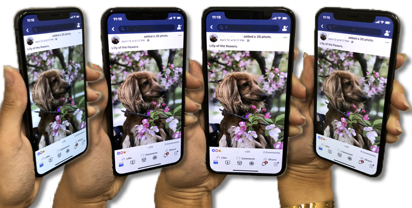
[Rotating phone induces parallax through sensing from the gyro.]Rotating phone induces parallax through sensing from the gyro.

Without motion, a 3D photo is just a 2D photo. Fully experiencing the 3D format requires moving the virtual viewpoint to recreate the parallax one would see in the real world. We have designed interfaces for both mobile devices and desktop browsers, as well as for head-mounted VR displays, where we also leverage stereo viewing.

5.1. Mobile and Browser

On mobile devices, there are a number of possible affordances that can be mapped to virtual camera motion. These include scrolling in the application interface, using the device’s IMUs such as the gyros to detect rotation, and using touch to manually rotate the view.

After considerable user testing, mapping scrolling behavior to both vertical rotation (about the horizontal axis) as well as dollying in and out (translation along the “z” axis) emerged as the best set of control interactions. This gives the illusion while scrolling through a vertical feed that the viewing point moves up and into the scene. We also added a small bit of horizontal rotation (about the vertical axis) mapped to scrolling. Furthermore, we add additional rotation to the virtual camera based on rotation of the device detected by gyros (see Figure 11). In a web browser, we substitute mouse motion for gyro rotation.

5.2. In Virtual Reality

In VR, we have the advantage of being able to produce two offset images, one for each eye, to enable binocular stereo. This creates a stronger feeling of immersion. 3D photos are currently the only photographic user-generated content in VR that makes use of all degrees of freedom in this medium.

We use threeJS (a Javascript 3D library) to render the scene to a WebGL context, and we use WebVR to render this context to a VR Device. The renderer queries the device parameters (eye buffer size and transforms), applying the information separately for the left and right eye views to produce a stereo image.

In addition to stereo, we map head motion directly to virtual camera motion. In 6-DOF headsets, this is a one-to-one mapping. In 3-DOF (rotation only), we mimic head translation from rotation around the neck since rotating the head to the left, for example, also translates the eyes leftward.

We create a frame around the model to hide the outer boundary of the photo. The result appears like a 3D model viewed through a 2D frame. Since the quality of the 3D photo display degrades when moving too far away from the original viewpoint, we constrain the viewing angles and fade the model out if there is too much head motion.

6. Results and Evaluation

6.1. Results

We have extensively tested the robustness of our system. Early versions of the system have been deployed in a social media app, where they have been used over 100 million times, attesting to the quality and robustness of the algorithms.

Unlike most other view synthesis methods our systems takes only a single color image as input. We can therefore apply it to any pre-existing image. In the supplementary video we show results on a wide range of historically significant photographs. We also show a large variety of results on snapshots.

6.2. Code

Pretrained models of our depth estimation network and inpainting networks are publicly available at the project page.

6.3. Performance

The table below breaks out the runtime of our algorithm stages on a typical image. We measured these numbers on an iPhone 11 Pro on six randomly selected $1152\times 1536$ images. Depth is estimated at $288\times 384$ resolution in 230ms. We report the median time for each stage.

Algorithm stage	Mean Runtime
Depth estimation	230ms
Depth filter	51ms
Connecting components	12ms
Occluded geometry	31ms
Color inpainting	540ms
Texture chart generation	72ms
Texture chart padding	151ms
Meshing	11ms
Total	1098ms

We store the final textured mesh in a GL Transmission Format (glTF) container for transmission. This representation can be rendered practically on device using standard graphics engines as discussed in Section 5. The final size of the textured mesh representation is typically around 300-500kb for an input image of size $1152\times 1536$.

An important advantage of our representation is that it is uses GPU memory efficiently. While an MPI stores a stack of full-sized images, the texture atlas only represents surfaces that are actually used.

6.4. Depth Estimation

Table 1. Quantitative evaluation our our depth estimation network. The best performance in each column is set in bold, and the second best underscored. Note, that for the quality evaluation every network used its preferred resolution, while for the performance evaluation we used a fixed resolution of $384\times 288$ for all networks. Please refer to the text for a detailed explanation.

Quality (MegaDepth) Quality (ReDWeb) Performance Model footprint Method Training data $\delta\!<\!1.25\!\uparrow$ Abs rel$\downarrow$ RMSE$\downarrow$ $\delta\!<\!1.25\!\uparrow$ Abs rel$\downarrow$ RMSE$\downarrow$ FLOPs$\downarrow$ Runtime$\downarrow$ Peak mem.$\downarrow$ float32 int8 Size$\downarrow$ Midas (v1) RW, MD, MV 0.955 0.068 $0.027$ - - - $33.2\text{\,}\mathrm{G}$ $1.11\text{\,}\mathrm{s}$ $453.7\text{\,}\mathrm{MiB}$ $37.3\text{\,}\mathrm{M}$ - $142.4\text{\,}\mathrm{MiB}$ Midas (v2) RW, DL, MV, MD, WSVD 0.965 0.058 0.022 - - - $72.3\text{\,}\mathrm{G}$ - - $104.0\text{\,}\mathrm{M}$ - $396.6\text{\,}\mathrm{MiB}$ Monodepth2 K $0.845$ $0.145$ $0.049$ $0.350$ $4.368$ $0.176$ $6.7\text{\,}\mathrm{G}$ $0.26\text{\,}\mathrm{s}$ $194.1\text{\,}\mathrm{MiB}$ $14.3\text{\,}\mathrm{M}$ - $54.6\text{\,}\mathrm{MiB}$ SharpNet PBRS $\rightarrow$ NYUv2 $0.839$ $0.146$ $0.051$ $0.308$ $6.616$ $0.196$ $54.9\text{\,}\mathrm{G}$ - - $114.1\text{\,}\mathrm{M}$ - $435.1\text{\,}\mathrm{MiB}$ MegaDepth DIW $\rightarrow$ MD $0.929$ $0.086$ $0.033$ 0.434 $2.270$ 0.137 $63.2\text{\,}\mathrm{G}$ - - $5.3\text{\,}\mathrm{M}$ - $20.4\text{\,}\mathrm{MiB}$ Ken Burns MD, NYUv2, KB $0.948$ $0.070$ 0.026 0.438 $2.968$ 0.140 $59.4\text{\,}\mathrm{G}$ - - $99.9\text{\,}\mathrm{M}$ - $381.0\text{\,}\mathrm{MiB}$ PyD-Net CS $\rightarrow$ K $0.836$ $0.148$ $0.052$ $0.310$ $5.218$ $0.198$ - - - $2.0\text{\,}\mathrm{M}$ - $7.9\text{\,}\mathrm{MiB}$ Tiefenrausch (baseline) MD $0.942$ $0.078$ $0.031$ $0.383$ $1.961$ $0.156$ $18.9\text{\,}\mathrm{G}$ - - $3.0\text{\,}\mathrm{M}$ - $11.4\text{\,}\mathrm{MiB}$ Tiefenrausch (AS + no-quant) MD $0.940$ $0.080$ $0.031$ $0.378$ $1.987$ $0.157$ $6.4\text{\,}\mathrm{G}$ - - $3.5\text{\,}\mathrm{M}$ - $13.4\text{\,}\mathrm{MiB}$ Tiefenrausch (AS + quant) MD $0.941$ $0.079$ $0.031$ $0.382$ 1.950 $0.156$ $6.4\text{\,}\mathrm{G}$ $0.23\text{\,}\mathrm{s}$ $196.1\text{\,}\mathrm{MiB}$ - $3.5\text{\,}\mathrm{M}$ $3.3\text{\,}\mathrm{MiB}$ Tiefenrausch (AS + quant) MD, 3DP $0.925$ $0.090$ $0.035$ $0.407$ 1.541 $0.142$ $6.4\text{\,}\mathrm{G}$ $0.23\text{\,}\mathrm{s}$ $196.1\text{\,}\mathrm{MiB}$ - $3.5\text{\,}\mathrm{M}$ $3.3\text{\,}\mathrm{MiB}$

We quantitatively compare our optimized depth estimation network against several state-of-the-baselines methods in Table 1. For most methods the authors only provided fine-tuned models and no training code. We list for each method the datasets it was trained with. In the training data column RW refers to ReDWeb (Xian et al., 2018), MD to MegaDepth (Li and Snavely, 2018), MV to Stereo Movies (Ranftl et al., 2019), DL to DIML Indoor (Kim et al., 2018), K to KITTI (Menze and Geiger, 2015), KB to Ken Burns (Niklaus et al., 2019), CS to Cityscapes (Cordts et al., 2016), WSVD (Wang et al., 2019), PBRS (Zhang et al., 2017), and NYUv2 (Silberman et al., 2012). 3DP refers to a proprietary dataset of 2.0M iPhone dual-camera images of a wide variety of scenes. A $\rightarrow$ B indicates that a model was pretrained on A and fine-tuned on B.

We compare against Midas (Ranftl et al., 2019) (versions 1 and 2 released in June 2019 and December 2019, respectively), Monodepth2 (Godard et al., 2019), SharpNet (Ramamonjisoa and Lepetit, 2019), MegaDepth (Li and Snavely, 2018), Ken Burns (Niklaus et al., 2019), and PyD-Net (Poggi et al., 2018).

Each method has a preferred resolution at which it performs best. These numbers are either explicitly listed in the respective papers or the author-provided code resizes inputs to the specific resolution. Also, different methods have different alignment requirements (e.g., width/height must be a multiple of 16). We list these details in the supplementary document, but briefly: all methods, except Monodepth2, Ken Burns, and PyD-Net resize the input image so the long dimension is 384 and the other dimension is resized to preserve the aspect ratio. Ken Burns and PyD-Net resize the long dimension to 1024 and 512, respectively, and Monodepth2 uses a fixed $1024\times 320$ aspect ratio. For this evaluation we resize the input image to each algorithm’s preferred resolution, and then resize the result to 384 pixels at which we compare against GT. We evaluate models on the MegaDepth test split (Li and Snavely, 2018) as well as the entire ReDWeb dataset (Wang et al., 2019), and report standard metrics. In the supplementary document we provide a larger number of standard metrics. For the Midas networks we omit the ReDWeb numbers because it was trained on this dataset, and ReDWeb does not provide a test split.

We evaluate four versions of our depth network:

Baseline::

refers to a manually crafted architecture, as described in Section 4.1.

AS + no-quant::

refers to an optimized architecture with float32 operators (i.e., no quantization).

AS + quant::

refers to the optimized architecture with quantization. This is our full model.

AS + quant, MD + 3DP::

for completeness we list another snapshot that was trained with a proprietary dataset of 2.0M dual-camera images.

We evaluate the performance on an example image of dimensions 384$\times$288. We first report the FLOP count of the model, computed analytically from the network schematics. Because FLOP counts do not always accurately reflect latency, we make runtime measurements on a mobile device. At the same time, we measure peak memory consumption during the inference. All models were run on an iPhone 11 Pro. We ran the models on the device as follows. All models came in PyTorch format (except PyD-Net). We converted them to Caffe2 using ONNX, because of Caffe2’s mobile capabilities (Caffe2go). We optimized the memory usage with the Caffe2 Memonger module. Because our scripts did not work on the PyD-Net tensorflow model we omit it from the performance evaluation. Then we measured the peak memory consumption by hooking the Caffe2 allocator function and keeping track of the maximum total allocation during the network run. Only Midas v1, Monodepth2, and our models were able to run on device, the other ones failed due to insufficient memory. Both models have footprints that are more than an order of magnitude larger than ours.

Finally, we provide details about the model size. We list the number of float32 and int8 parameters for each model as well as the total model size in MiB, with smaller models being more amendable to mobile download. While our method does not perform best in terms of quality compared to significantly higher number of parameter state of the art models, it is competitive and the quality is sufficient for our intended application, as demonstrated by hundreds of results shown in the supplemental video. The main advantages of our model is that its size is significantly smaller also resulting in significantly reduced computation compared to the state of the art models. The enables depth estimation even on older phone hardware.

6.5. Inpainting

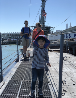
(a) Original view, ground truth

$\underbracket{\parbox[t]{103.3461pt}{\vspace{0mm}\centering\leavevmode\hbox{\set@color\vspace{0mm}\centering\framebox{\includegraphics[height=119.50148pt,trim=0.0pt 150.5625pt 0.0pt 0.0pt,clip]{figures/inpaint_eval_repro/nv_gt_L0}}\@add@centering}\\ \vspace{\vneg}\small(b) First layer, ground truth\@add@centering}\hskip 2.84526pt\parbox[t]{103.3461pt}{\vspace{0mm}\centering\leavevmode\hbox{\set@color\vspace{0mm}\centering\framebox{\includegraphics[height=119.50148pt,trim=0.0pt 150.5625pt 0.0pt 0.0pt,clip]{figures/inpaint_eval_repro/nv_gt_L1}}\@add@centering}\\ \vspace{\vneg}\small(c) Second layer, ground truth\@add@centering}\hskip 2.84526pt\parbox[t]{103.3461pt}{\vspace{0mm}\centering\leavevmode\hbox{\set@color\vspace{0mm}\centering\framebox{\includegraphics[height=119.50148pt,trim=0.0pt 150.5625pt 0.0pt 0.0pt,clip]{figures/inpaint_eval_repro/nv_inpainted_L1}}\@add@centering}\\ \vspace{\vneg}\small(d) Second layer, Inpainted\@add@centering}}_{\begin{subarray}{c}\vspace{-3.5mm}\\ \hbox{\pagecolor{white}~{}~{}\small Novel view~{}~{}}\end{subarray}}$ (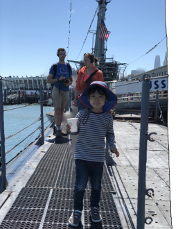e) Original view, inpainted

Figure 12. Inpainting evaluation. In order to evaluate inpainting we follow this procedure: left input image to single-layer LDI (i.e., no extending)

(a) Ground truth

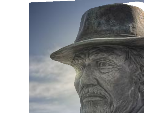
(b) Wrapped view

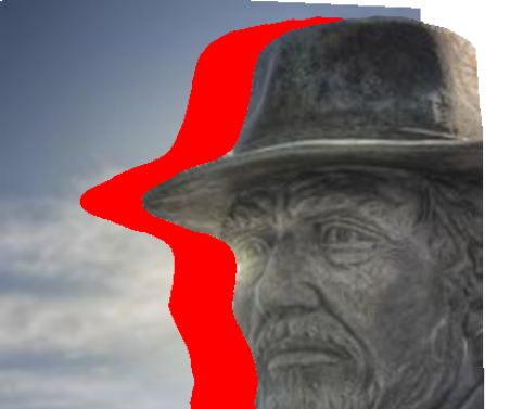
(c) Masked input

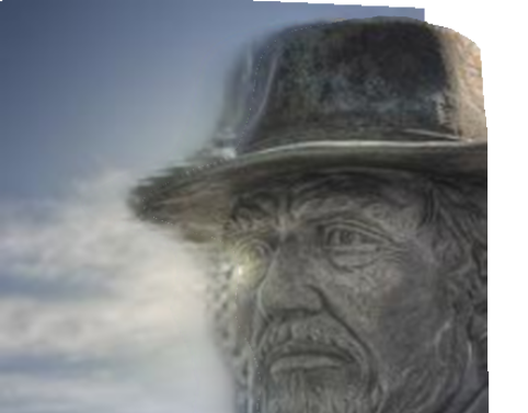
(d) Farbrausch screen space inpainting

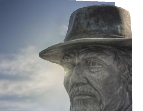
(e) Farbrausch LDI inpainting

Figure 13. Comparing screen space inpainting to our LDI space inpainting using the same network (Farbrausch) trained on 2D images. Source image © flickr user -ytf-, https://www.flickr.com/photos/ytf/6837709270/, used with permission.

Table 2. Inpainting Evaluation. The best performance in each column is set in bold, and the second best underscored. Note, FLOP count depends on the input size, and in the case of LDI this number is variable depending upon the geometric complexity; we report FLOP counts for screen space inpainting with an image resolution of $512\times 512$.

	Quality (LDI)	Quality (reprojected)			Performance	Model footprint
Method	PSNR$\uparrow$	PSNR$\uparrow$	SSIM$\uparrow$	LPIPS$\downarrow$	FLOPs$\downarrow$	float32$\downarrow$	Caffe2 Size$\downarrow$
Farbrausch	33.852	34.126	0.9829	0.0232	-	$0.37\text{\,}\mathrm{M}$	$1.9\text{\,}\mathrm{MiB}$
Partial Convolution	33.795	34.001	0.9832	0.0224	-	$32.85\text{\,}\mathrm{M}$	$164.4\text{\,}\mathrm{MiB}$
Farbrausch (screen space)	-	32.0211	0.9784	0.0325	$2.56\text{\,}\mathrm{G}$	$0.37\text{\,}\mathrm{M}$	$1.9\text{\,}\mathrm{MiB}$
Partial Convolution (screen space)	-	33.225	0.9807	0.0280	$37.97\text{\,}\mathrm{G}$	$32.85\text{\,}\mathrm{M}$	$164.4\text{\,}\mathrm{MiB}$

We quantitatively evaluate inpainting on the ReDWeb dataset (Xian et al., 2018), because it has dense depth supervision. In order to evaluate inpainting we follow this procedure:

• For each image in the dataset we lift input image to single-layer LDI (i.e., no extending) and use micro-polygons. That is, we capture all detail, but we don’t hallucinate any new details. (Figure 12a).

• Then we render the image from a canonical viewpoint and use depth peeling to obtain an LDI with known colors at all layers, not just the first one (Figure 12b–c show the first two layers).

• We consider all layers except the first one as unknown and inpaint them (Figure 12d).

• Finally, we reproject the inpainted LDI back to the original view (Figure 12e). This is useful, because in this view all inpainted pixels (from any LDI layer) are visible, and because it is a normal rendered image we can use any image-space metric.

In the “Quality (LDI)” column in Table 2 we report a quality loss computed on the LDI (i.e., between Figures 12c and 12d). In the “Quality (reprojected)” column in Table 2 we report PSNR and SSIM metrics. Since SSIM and PSNR evaluate for reconstruction error, we also include the LPIPS metric (Zhang et al., 2018) to better evaluate the perceptual similarity of the inpainted image compared to the ground truth.

We compare our optimized model against original full size PartialConv model. We also compare against using both models applied in regular screen space inpainting. Fig. 13 illustrates the significant artifacts on the edges when naively using regular screen space inpainting.

6.6. End-to-end View Synthesis

In the supplementary material we provide a qualitative comparison to the “3D Ken Burns Effect” (Niklaus et al., 2019). Note that the output of that system is a video showing a linear camera trajectory, and their inpainting is optimized solely for viewpoints along that trajectory. In contrast, the output of our system is a mesh that is suitable for rendering from any viewpoint near the point of capture.

6.7. Limitations

As with any computer vision method, our algorithm does not always work perfectly. The depth estimation degrades in situations that are not well represented in the training data. An inherent limitation of the depth representation is that there is only one depth value per pixel in the input; semi-transparent surfaces or participating media (e.g., fog or smoke) are not well represented. We thus see a number of cases where the resulting 3D photo suffers from bad depth values. Nevertheless, most scene captures do result in successful 3D photos. The sets of images in the two “results” parts in the supplemental video, were only selected for content before applying our algorithm. We did not remove any failure cases based on processing. Therefore, you can see some artifacts if examined closely. They thus provide an idea of the success rate of the algorithm.

7. Conclusions and future work

In this work, we presented a new medium, a 3D Photo, and a system to produce them on any mobile device starting from a single image. These 3D photos can be consumed on any mobile device as well through desktop browsers. Scrolling, device motion, or mouse motion all induce virtual viewpoint change and thereby motion parallax. 3D Photos also are viewable in HMDs enabling stereoscopic viewing responsive to head motion.

Not only have we described the steps necessary to produce 3D Photos, but we’ve also presented advancements in optimizing depth and inpainting neural networks to run more efficiently on mobile devices. These advancements can be used to improve fundamental algorithmic building blocks for Augmented Reality experiences.

There are many avenues for exploring human-in-the-loop creative expression with the 3D photo format. While this work shows how to auto-generate a 3D photo using real imagery, a future direction is to build out a rich set of creative tools to accommodate artistic intent.

References

- (1)
- Chen et al. (2016) Weifeng Chen, Zhao Fu, Dawei Yang, and Jia Deng. 2016. Single-image depth perception in the wild. In Advances in Neural Information Processing Systems. 730–738.
- Choi et al. (2018) Jungwook Choi, Zhuo Wang, Swagath Venkataramani, Pierce I-Jen Chuang, Vijayalakshmi Srinivasan, and Kailash Gopalakrishnan. 2018. Pact: Parameterized clipping activation for quantized neural networks. arXiv preprint arXiv:1805.06085 (2018).
- Cordts et al. (2016) Marius Cordts, Mohamed Omran, Sebastian Ramos, Timo Rehfeld, Markus Enzweiler, Rodrigo Benenson, Uwe Franke, Stefan Roth, and Bernt Schiele. 2016. The Cityscapes Dataset for Semantic Urban Scene Understanding. In Proc. of the IEEE Conference on Computer Vision and Pattern Recognition (CVPR).
- Dai et al. (2019) Xiaoliang Dai, Yangqing Jia, Peter Vajda, Matt Uyttendaele, Niraj K. Jha, Peizhao Zhang, Bichen Wu, Hongxu Yin, Fei Sun, Yanghan Wang, and et al. 2019. ChamNet: Towards Efficient Network Design Through Platform-Aware Model Adaptation. In IEEE Conference on Computer Vision and Pattern Recognition (CVPR).
- de Berg et al. (2008) Mark de Berg, Otfried Cheong, Marc van Kreveld, and Mark Overmars. 2008. Computational Geometry: Algorithms and Applications (3rd ed. ed.). Springer-Verlag TELOS, Santa Clara, CA, USA.
- Douglas and Peucker (1973) David Douglas and Thomas Peucker. 1973. Algorithms for the Reduction of the Number of Points Required to Represent a Digitized Line or Its Caricature. Cartographica: The International Journal for Geographic Information and Geovisualization 10 (1973), 112–122.
- Flynn et al. (2019) John Flynn, Michael Broxton, Paul Debevec, Matthew DuVall, Graham Fyffe, Ryan Overbeck, Noah Snavely, and Richard Tucker. 2019. DeepView: View Synthesis With Learned Gradient Descent. In The IEEE Conference on Computer Vision and Pattern Recognition (CVPR).
- Garg et al. (2016) Ravi Garg, Vijay Kumar B.G., Gustavo Carneiro, and Ian Reid. 2016. Unsupervised CNN for Single View Depth Estimation: Geometry to the Rescue. In Computer Vision – ECCV 2016. 740–756.
- Godard et al. (2017) Clément Godard, Oisin Mac Aodha, and Gabriel J. Brostow. 2017. Unsupervised Monocular Depth Estimation with Left-Right Consistency. In IEEE Conference on Computer Vision and Pattern Recognition (CVPR).
- Godard et al. (2019) Clément Godard, Oisin Mac Aodha, Michael Firman, and Gabriel J. Brostow. 2019. Digging into Self-Supervised Monocular Depth Prediction. In International Conference on Computer Vision (ICCV).
- Hedman et al. (2017) Peter Hedman, Suhib Alsisan, Richard Szeliski, and Johannes Kopf. 2017. Casual 3D Photography. ACM Trans. Graph. 36, 6 (2017), article no. 234.
- Hedman and Kopf (2018) Peter Hedman and Johannes Kopf. 2018. Instant 3D Photography. ACM Trans. Graph. 37, 4 (2018), article no. 101.
- Horry et al. (1997) Youichi Horry, Ken-Ichi Anjyo, and Kiyoshi Arai. 1997. Tour into the Picture: Using a Spidery Mesh Interface to Make Animation from a Single Image. In Proceedings of the 24th Annual Conference on Computer Graphics and Interactive Techniques (SIGGRAPH ’97). 225–232.
- Jacob et al. (2018) Benoit Jacob, Skirmantas Kligys, Bo Chen, Menglong Zhu, Matthew Tang, Andrew Howard, Hartwig Adam, and Dmitry Kalenichenko. 2018. Quantization and training of neural networks for efficient integer-arithmetic-only inference. In Proceedings of the IEEE Conference on Computer Vision and Pattern Recognition. 2704–2713.
- Kim et al. (2018) Youngjung Kim, Hyungjoo Jung, Dongbo Min, and Kwanghoon Sohn. 2018. Deep Monocular Depth Estimation via Integration of Global and Local Predictions. IEEE Transactions on Image Processing 27, 8 (2018), 4131–4144.
- Kuznietsov et al. (2017) Yevhen Kuznietsov, Jorg Stuckler, and Bastian Leibe. 2017. Semi-Supervised Deep Learning for Monocular Depth Map Prediction. In The IEEE Conference on Computer Vision and Pattern Recognition (CVPR).
- Li and Snavely (2018) Zhengqi Li and Noah Snavely. 2018. MegaDepth: Learning Single-View Depth Prediction from Internet Photos. In Computer Vision and Pattern Recognition (CVPR).
- Lin et al. (2020) L. Lin, G. Huang, Y. Chen, L. Zhang, and B. He. 2020. Efficient and High-Quality Monocular Depth Estimation via Gated Multi-Scale Network. IEEE Access 8 (2020), 7709–7718.
- Liu et al. (2018b) Guilin Liu, Fitsum A. Reda, Kevin J. Shih, Ting-Chun Wang, Andrew Tao, and Bryan Catanzaro. 2018b. Image Inpainting for Irregular Holes Using Partial Convolutions. In The European Conference on Computer Vision (ECCV).
- Liu et al. (2018c) Guilin Liu, Kevin J. Shih, Ting-Chun Wang, Fitsum A. Reda, Karan Sapra, Zhiding Yu, Andrew Tao, and Bryan Catanzaro. 2018c. Partial Convolution based Padding. In arXiv preprint arXiv:1811.11718.
- Liu et al. (2018a) Miaomiao Liu, Xuming He, and Mathieu Salzmann. 2018a. Geometry-Aware Deep Network for Single-Image Novel View Synthesis. In 2018 IEEE Conference on Computer Vision and Pattern Recognition, CVPR. 4616–4624.
- Martin-Brualla et al. (2018) Ricardo Martin-Brualla, Rohit Pandey, Shuoran Yang, Pavel Pidlypenskyi, Jonathan Taylor, Julien Valentin, Sameh Khamis, Philip Davidson, Anastasia Tkach, Peter Lincoln, Adarsh Kowdle, Christoph Rhemann, Dan B Goldman, Cem Keskin, Steve Seitz, Shahram Izadi, and Sean Fanello. 2018. LookinGood: Enhancing Performance Capture with Real-time Neural Re-rendering. ACM Trans. Graph. 37, 6 (2018), article no. 255.
- Menze and Geiger (2015) Moritz Menze and Andreas Geiger. 2015. Object Scene Flow for Autonomous Vehicles. In IEEE Conf. on Computer Vision and Pattern Recognition (CVPR) 2015. 3061–3070.
- Meshry et al. (2019) Moustafa Meshry, Dan B Goldman, Sameh Khamis, Hugues Hoppe, Rohit Pandey, Noah Snavely, and Ricardo Martin-Brualla. 2019. Neural Rerendering in the Wild. arXiv preprint (2019).
- Mildenhall et al. (2019) Ben Mildenhall, Pratul P. Srinivasan, Rodrigo Ortiz-Cayon, Nima Khademi Kalantari, Ravi Ramamoorthi, Ren Ng, and Abhishek Kar. 2019. Local Light Field Fusion: Practical View Synthesis with Prescriptive Sampling Guidelines. ACM Transactions on Graphics (TOG) (2019).
- Niklaus et al. (2019) Simon Niklaus, Long Mai, Jimei Yang, and Feng Liu. 2019. 3D Ken Burns Effect from a Single Image. ACM Transactions on Graphics 38, 6 (2019), article no. 184.
- Oh et al. (2001) Byong Mok Oh, Max Chen, Julie Dorsey, and Frédo Durand. 2001. Image-based Modeling and Photo Editing. In Proceedings of the 28th Annual Conference on Computer Graphics and Interactive Techniques (SIGGRAPH ’01). 433–442.
- Peluso et al. (2019) V. Peluso, A. Cipolletta, A. Calimera, M. Poggi, F. Tosi, and S. Mattoccia. 2019. Enabling Energy-Efficient Unsupervised Monocular Depth Estimation on ARMv7-Based Platforms. In 2019 Design, Automation Test in Europe Conference Exhibition (DATE). 1703–1708.
- Poggi et al. (2018) Matteo Poggi, Filippo Aleotti, Fabio Tosi, and Stefano Mattoccia. 2018. Towards real-time unsupervised monocular depth estimation on CPU. In IEEE/JRS Conference on Intelligent Robots and Systems (IROS).
- Ramamonjisoa and Lepetit (2019) Michael Ramamonjisoa and Vincent Lepetit. 2019. SharpNet: Fast and Accurate Recovery of Occluding Contours in Monocular Depth Estimation. The IEEE International Conference on Computer Vision (ICCV) Workshops (2019).
- Ranftl et al. (2019) René Ranftl, Katrin Lasinger, David Hafner, Konrad Schindler, and Vladlen Koltun. 2019. Towards Robust Monocular Depth Estimation: Mixing Datasets for Zero-shot Cross-dataset Transfer. arXiv:1907.01341 (2019).
- Ronneberger et al. (2015) Olaf Ronneberger, Philipp Fischer, and Thomas Brox. 2015. U-Net: Convolutional Networks for Biomedical Image Segmentation. Medical Image Computing and Computer-Assisted Intervention – MICCAI 2015 (2015), 234–241.
- Sandler et al. (2018) Mark Sandler, Andrew Howard, Menglong Zhu, Andrey Zhmoginov, and Liang-Chieh Chen. 2018. MobileNetV2: Inverted Residuals and Linear Bottlenecks. In The IEEE Conference on Computer Vision and Pattern Recognition (CVPR).
- Saxena et al. (2006) Ashutosh Saxena, Sung H. Chung, and Andrew Y. Ng. 2006. Learning Depth from Single Monocular Images. Advances in Neural Information Processing Systems 18 (2006), 1161–1168.
- Shade et al. (1998) Jonathan Shade, Steven Gortler, Li-wei He, and Richard Szeliski. 1998. Layered Depth Images. In Proceedings of the 25th Annual Conference on Computer Graphics and Interactive Techniques (SIGGRAPH ’98). 231–242.
- Silberman et al. (2012) Nathan Silberman, Derek Hoiem, Pushmeet Kohli, and Rob Fergus. 2012. Indoor Segmentation and Support Inference from RGBD Images. In European Conference on Computer Vision (ECCV).
- Sitzmann et al. (2019) Vincent Sitzmann, Justus Thies, Felix Heide, Matthias Nießner, Gordon Wetzstein, and Michael Zollhöfer. 2019. DeepVoxels: Learning Persistent 3D Feature Embeddings. In Proc. Computer Vision and Pattern Recognition (CVPR), IEEE.
- Srinivasan et al. (2019) Pratul P. Srinivasan, Richard Tucker, Jonathan T. Barron, Ravi Ramamoorthi, Ren Ng, and Noah Snavely. 2019. Pushing the Boundaries of View Extrapolation with Multiplane Images. In IEEE Conference on Computer Vision and Pattern Recognition (CVPR).
- Srinivasan et al. (2017) Pratul P. Srinivasan, Tongzhou Wang, Ashwin Sreelal, Ravi Ramamoorthi, and Ren Ng. 2017. Learning to Synthesize a 4D RGBD Light Field from a Single Image. In IEEE International Conference on Computer Vision, ICCV. 2262–2270.
- Tonioni et al. (2019) A. Tonioni, F. Tosi, M. Poggi, S. Mattoccia, and L. D. Stefano. 2019. Real-Time Self-Adaptive Deep Stereo. In 2019 IEEE/CVF Conference on Computer Vision and Pattern Recognition (CVPR). 195–204.
- Wang et al. (2019) Chaoyang Wang, Simon Lucey, Federico Perazzi, and Oliver Wang. 2019. Web Stereo Video Supervision for Depth Prediction from Dynamic Scenes. In International Conference on 3D Vision (3DV).
- Wofk et al. (2019) Diana Wofk, Fangchang Ma, Tien-Ju Yang, Sertac Karaman, and Vivienne Sze. 2019. FastDepth: Fast Monocular Depth Estimation on Embedded Systems. In IEEE International Conference on Robotics and Automation (ICRA).
- Wu et al. (2019) Bichen Wu, Xiaoliang Dai, Peizhao Zhang, Yanghan Wang, Fei Sun, Yiming Wu, Yuandong Tian, Peter Vajda, Yangqing Jia, and Kurt Keutzer. 2019. FBNet: Hardware-Aware Efficient ConvNet Design via Differentiable Neural Architecture Search. In IEEE Conference on Computer Vision and Pattern Recognition (CVPR).
- Xian et al. (2018) Ke Xian, Chunhua Shen, Zhiguo Cao, Hao Lu, Yang Xiao, Ruibo Li, and Zhenbo Luo. 2018. Monocular Relative Depth Perception With Web Stereo Data Supervision. In IEEE Conference on Computer Vision and Pattern Recognition (CVPR).
- Zhang et al. (2018) Richard Zhang, Phillip Isola, Alexei A. Efros, Eli Shechtman, and Oliver Wang. 2018. The Unreasonable Effectiveness of Deep Features as a Perceptual Metric. In IEEE Conference on Computer Vision and Pattern Recognition (CVPR).
- Zhang et al. (2017) Yinda Zhang, Shuran Song, Ersin Yumer, Manolis Savva, Joon-Young Lee, Hailin Jin, and Thomas Funkhouser. 2017. Physically-Based Rendering for Indoor Scene Understanding Using Convolutional Neural Networks. In IEEE Conference on Computer Vision and Pattern Recognition (CVPR).
- Zhao et al. (2017) Hengshuang Zhao, Jianping Shi, Xiaojuan Qi, Xiaogang Wang, and Jiaya Jia. 2017. Pyramid scene parsing network. In IEEE Conference on Computer Vision and Pattern Recognition (CVPR). 2881–2890.
- Zhou et al. (2018) Tinghui Zhou, Richard Tucker, John Flynn, Graham Fyffe, and Noah Snavely. 2018. Stereo Magnification: Learning View Synthesis Using Multiplane Images. ACM Transactions on Graphics (TOG) 37, 4 (2018), article no. 65.
- Zitnick et al. (2004) C. Lawrence Zitnick, Sing Bing Kang, Matthew Uyttendaele, Simon Winder, and Richard Szeliski. 2004. High-quality Video View Interpolation Using a Layered Representation. ACM Trans. Graph. 23, 3 (2004), 600–608.