Understanding and Detecting Convergence for Stochastic Gradient Descent with Momentum

Jerry Chee,Β  Ping Li Cognitive Computing Lab
Baidu Research
10900 NE 8th St. Bellevue, WA 98004, USA
jerry9567@gmail.com, ping98@gmail.com
Abstract

Convergence detection of iterative stochastic optimization methods is of great practical interest. This paper considers stochastic gradient descent (SGD) with a constant learning rate and momentum. We show that there exists a transient phase in which iterates move towards a region of interest, and a stationary phase in which iterates remain bounded in that region around a minimum point. We construct a statistical diagnostic test for convergence to the stationary phase using the inner product between successive gradients and demonstrate that the proposed diagnostic works well. We theoretically and empirically characterize how momentum can affect the test statistic of the diagnostic, and how the test statistic captures a relatively sparse signal within the gradients in convergence. Finally, we demonstrate an application to automatically tune the learning rate by reducing it each time stationarity is detected, and show the procedure is robust to mis-specified initial rates.

I Introduction

Consider the problem in stochastic optimization

θ⋆subscriptπœƒβ‹†\displaystyle\theta_{\star} =arg⁑minΞΈβˆˆΞ˜β‘π”Όβ€‹[ℓ​(ΞΈ,ΞΎ)].absentsubscriptπœƒΞ˜π”Όdelimited-[]β„“πœƒπœ‰\displaystyle=\arg\min_{\theta\in\Theta}\mathbb{E}[\ell(\theta,\xi)]. (1)

The loss β„“β„“\ell is parameterized by Ξ˜βŠ†β„pΘsuperscriptℝ𝑝\Theta\subseteq\mathbb{R}^{p}, and ΞΎπœ‰\xi is a source of randomness like a randomly sampled point. For example, the quadratic loss is ℓ​(ΞΈ,ΞΎ)=(1/2)​(yβˆ’xβŠ€β€‹ΞΈ)2β„“πœƒπœ‰12superscript𝑦superscriptπ‘₯topπœƒ2\ell(\theta,\xi)=(1/2)(y-x^{\top}\theta)^{2} with ΞΎ=(x,y)πœ‰π‘₯𝑦\xi=(x,y). When the data size N𝑁N and parameter size p𝑝p are large, classical optimization methods can fail to estimate θ⋆subscriptπœƒβ‹†\theta_{\star}. In such large-scale settings stochastic gradient descent (SGD):

ΞΈn+1=ΞΈnβˆ’Ξ³β€‹βˆ‡β„“β€‹(ΞΈn,ΞΎn+1)subscriptπœƒπ‘›1subscriptπœƒπ‘›π›Ύβˆ‡β„“subscriptπœƒπ‘›subscriptπœ‰π‘›1\theta_{n+1}=\theta_{n}-\gamma\nabla\ell(\theta_{n},\xi_{n+1}) (2)

is a powerful alternativeΒ [4, 5, 34, 30]. ΞΈn+1subscriptπœƒπ‘›1\theta_{n+1} is the estimate of θ⋆subscriptπœƒβ‹†\theta_{\star} at the (n+1)𝑛1(n+1)-th iteration, and Ξ³>0𝛾0\gamma>0 the learning rate. ΞΎn+1subscriptπœ‰π‘›1\xi_{n+1} represents randomly sampled data used to compute the stochastic gradient. A mini-batch can reduce the variance of the stochastic gradients and aid in performanceΒ [25].

Momentum or Heavy Ball SGD (SGDM) can offer significant speedupsΒ [24]:

ΞΈn+1=ΞΈnβˆ’Ξ³β€‹βˆ‡β„“β€‹(ΞΈn,ΞΎn+1)+β​(ΞΈnβˆ’ΞΈnβˆ’1)subscriptπœƒπ‘›1subscriptπœƒπ‘›π›Ύβˆ‡β„“subscriptπœƒπ‘›subscriptπœ‰π‘›1𝛽subscriptπœƒπ‘›subscriptπœƒπ‘›1\theta_{n+1}=\theta_{n}-\gamma\nabla\ell(\theta_{n},\xi_{n+1})+\beta(\theta_{n}-\theta_{n-1}) (3)

where β∈[0,1)𝛽01\beta\in[0,1) is the momentum. The momentum term β​(ΞΈnβˆ’ΞΈnβˆ’1)𝛽subscriptπœƒπ‘›subscriptπœƒπ‘›1\beta(\theta_{n}-\theta_{n-1}) accumulates movements in a common direction. The performance of stochastic gradient methods is greatly influenced by the learning rate γ𝛾\gamma, which can be decreasing (e.g., ∝1/nproportional-toabsent1𝑛\propto 1/n) or constant. Decreasing learning rates are commonly used in the literature to attain theoretical convergence guarantees. However in practice constant learning rates are common due to their ease of tuning and speed of convergence.

Stochastic iterative procedures start from an initial point and then move from a transient phase to a stationary phaseΒ [20]. With a decreasing learning rate, the transient phase can be long, and impractically so if the learning rate is just slightly misspecifiedΒ [22, 31]. But, the stationary phase is convergence to θ⋆subscriptπœƒβ‹†\theta_{\star}. With a constant learning rate the transient phase is much shorter and more robust to the learning rate. The stationary phase is not true convergence but oscillation within a bounded region containing θ⋆subscriptπœƒβ‹†\theta_{\star}. In this study, we develop a statistical convergence diagnostic for SGDM with constant learning rate. Constant learning rate is commonly used in practice, makes the transition from transient to stationary phase clear, and it is pointless to keep running the procedure once the stationary phase has been reached.

I-A Related work

The idea that stochastic gradient methods can be separated into a transient and stationary phase (or search and convergence phase) is not newΒ [20]. However, until recently there has been little work in developing principled statistical methods for convergence detection which can guide empirical practice. Heuristics from optimization theory are commonly used, such as stopping when β€–ΞΈnβˆ’ΞΈnβˆ’1β€–normsubscriptπœƒπ‘›subscriptπœƒπ‘›1\|\theta_{n}-\theta_{n-1}\| is small according to some threshold, or when updates of the loss function have reached machine precisionΒ [6, 11]. These methods are more suited for deterministic rather than stochastic procedures as they do not account for the sampling variation in stochastic gradient estimates. A more statistically motivated approach is to concurrently monitor test error on a hold-out validation set and stop when validation error begins increasingΒ [3, 5]. But, the validation error is also a stochastic process, and estimating whether it is increasing presents similar, if not greater, challenges to detecting convergence to the stationaryΒ phase.

In stochastic approximation, classical theory of stopping times addresses the detection of stationarityΒ [23, 33]. One noteworthy method byΒ [23] forms the basis for our work. It keeps a running average of the inner product of successive gradients βˆ‡β„“β€‹(ΞΈn,ΞΎn+1)βŠ€β€‹βˆ‡β„“β€‹(ΞΈnβˆ’1,ΞΎn)βˆ‡β„“superscriptsubscriptπœƒπ‘›subscriptπœ‰π‘›1topβˆ‡β„“subscriptπœƒπ‘›1subscriptπœ‰π‘›\nabla\ell(\theta_{n},\xi_{n+1})^{\top}\nabla\ell(\theta_{n-1},\xi_{n}). At a high level, in the transient phase the stochastic gradients generally point in the same direction, resulting in a positive inner product. In the stationary phase the stochastic gradients roughly point in different directions due to their oscillation in a bounded region containing θ⋆subscriptπœƒβ‹†\theta_{\star}, resulting in a negative inner product. Accelerated methods in stochastic approximation share the underlying intuition that a negative inner product of successive gradients indicates convergenceΒ [10, 15, 26].

There has been recent interest in principled convergence detection for stochastic gradient methods, and automated step decay learning rates. Work byΒ [7] developed a principled convergence diagnostic for SGD in Eq.Β (2) based on Pflug’s procedure. We generalize Pflug’s procedure to the momentum setting, which introduces challenges to the theoretical justification and practicality of the convergence diagnostic.Β [14] developed a procedure to automatically switch from AdamΒ [16] to SGD.Β [27] propose a modified splitting procedureΒ [28] to detect the stationary phase for SGD and implement a robust learning rate schedule.Β [18] use a Markov chain t𝑑t-test and a stationarity condition byΒ [32] to automatically reduce the learning rate for SGDM.Β [12] analyze the step decay learning rate schedule in least squares regression and show its optimality over polynomially decaying rates.

I-B Our contributions

SectionΒ II presents a statistical convergence diagnostic for SGDM (stochastic gradient descent with momentum) and explains the significance of the challenges introduced by momentum. In SectionΒ III we provide theoretical and empirical support for the design choices of the convergence diagnostic, and demonstrate the effect of momentum on the test statistic of the diagnostic. We investigate in SectionΒ IV what drives the test statistic by analyzing the distribution of the inner product of successive gradients in the stationary phase. In SectionΒ V we provide empirical type I and type II error rates on simulated data experiments. SectionΒ VI presents an application of the convergence diagnostic to an automatically tuned learning rate schedule, with experiments on benchmark datasets.

II Convergence diagnostic

Our convergence diagnostic aims to detect the transition from the transient to the stationary phase. We first present theory which supports the existence of these two phases for SGDM. The expected difference in loss to the minimum has bias terms due to initial conditions, and a variance term due to noise in the stochastic gradients.

Theorem 1 ([29]).

If the expected loss f​(ΞΈ)=𝔼​[ℓ​(ΞΈ,ΞΎ)]π‘“πœƒπ”Όdelimited-[]β„“πœƒπœ‰f(\theta)=\mathbb{E}[\ell(\theta,\xi)] is convex, under additional assumptions of the loss, there are positive constants QΞ²,RΞ²,SΞ²subscript𝑄𝛽subscript𝑅𝛽subscript𝑆𝛽Q_{\beta},R_{\beta},S_{\beta} such that for every n𝑛n, we have

𝔼​[f​(ΞΈ^n)βˆ’f​(θ⋆)]𝔼delimited-[]𝑓subscript^πœƒπ‘›π‘“subscriptπœƒβ‹†\displaystyle\mathbb{E}[f(\hat{\theta}_{n})-f(\theta_{\star})] ≀QΞ²n+1​(f​(ΞΈ0)βˆ’f​(θ⋆))absentsubscript𝑄𝛽𝑛1𝑓subscriptπœƒ0𝑓subscriptπœƒβ‹†\displaystyle\leq\frac{Q_{\beta}}{n+1}(f(\theta_{0})-f(\theta_{\star}))
+Rβγ​(n+1)βˆ₯ΞΈ0βˆ’ΞΈβ‹†βˆ₯2+Ξ³SΞ².β–‘\displaystyle\quad+\frac{R_{\beta}}{\gamma(n+1)}\|\theta_{0}-\theta_{\star}\|^{2}+\gamma S_{\beta}.\hskip 14.45377pt\Box

Remarks. ΞΈ^n=βˆ‘t=0nΞΈt/(n+1)subscript^πœƒπ‘›superscriptsubscript𝑑0𝑛subscriptπœƒπ‘‘π‘›1\hat{\theta}_{n}=\sum_{t=0}^{n}\theta_{t}/(n+1), QΞ²=Ξ²/(1βˆ’Ξ²),RΞ²=(1βˆ’Ξ²)/2formulae-sequencesubscript𝑄𝛽𝛽1𝛽subscript𝑅𝛽1𝛽2Q_{\beta}=\beta/(1-\beta),R_{\beta}=(1-\beta)/2, and SΞ²=(G2+Ξ΄2)/2​(1βˆ’Ξ²)subscript𝑆𝛽superscript𝐺2superscript𝛿221𝛽S_{\beta}=(G^{2}+\delta^{2})/2(1-\beta) where G𝐺G is a bound on the gradients and Ξ΄2superscript𝛿2\delta^{2} a bound on the variance of the stochastic gradients. For large enough n𝑛n the bias contributions from the transient phase are negligible, and thus bounded 𝔼​[f​(ΞΈ^n)βˆ’f​(θ⋆)]𝔼delimited-[]𝑓subscript^πœƒπ‘›π‘“subscriptπœƒβ‹†\mathbb{E}[f(\hat{\theta}_{n})-f(\theta_{\star})] indicates a bounded 𝔼​[f​(ΞΈn)βˆ’f​(θ⋆)]𝔼delimited-[]𝑓subscriptπœƒπ‘›π‘“subscriptπœƒβ‹†\mathbb{E}[f(\theta_{n})-f(\theta_{\star})]Β inΒ theΒ stationaryΒ phase.

TheoremΒ 1 suggests that constant rate SGDM moves quickly through the transient phase discounting initial conditions f​(ΞΈ0)βˆ’f​(θ⋆)𝑓subscriptπœƒ0𝑓subscriptπœƒβ‹†f(\theta_{0})-f(\theta_{\star}) and β€–ΞΈ0βˆ’ΞΈβ‹†β€–2superscriptnormsubscriptπœƒ0subscriptπœƒβ‹†2\|\theta_{0}-\theta_{\star}\|^{2}, and then enters the stationary phase where the distance from θ⋆subscriptπœƒβ‹†\theta_{\star} is bounded ∝O​(Ξ³)proportional-toabsent𝑂𝛾\propto O(\gamma). We observe a widely noted trade-off for stochastic gradient methods: a larger learning rate speeds up the transient phase by discounting bias from initial conditions at a higher rate, but increases the radius of the stationary regionΒ [1, 21].

We citeΒ [29] in TheoremΒ 1 because their convergence rate consisting of a reducible and irreducible term with respect to the number of updates, and best matches our empirical observations. ThoughΒ [19] show a linear convergence rate with constant stepsize, their restriction on the momentum (β𝛽\beta) makes their convergence rate difficult to realize in practice. For example, using the formula inΒ [19] with min and max eigenvalues =0.5absent0.5=0.5 and stepsize =0.1absent0.1=0.1, Ξ²<0.2𝛽0.2\beta<0.2, whichΒ isΒ veryΒ restrictive.

While convergence analyses such as TheoremΒ 1 offer valuable theoretical insight, they provide limited practical guidance. One could try to declare convergence when the bias due to initial conditions has been discounted to 1%percent11\% of the variance, choosing n𝑛n for [QΞ²n+1​(f​(ΞΈ0)βˆ’f​(θ⋆))+Rβγ​(n+1)​‖θ0βˆ’ΞΈβ‹†β€–2]=0.01​γ​SΞ²delimited-[]subscript𝑄𝛽𝑛1𝑓subscriptπœƒ0𝑓subscriptπœƒβ‹†subscript𝑅𝛽𝛾𝑛1superscriptnormsubscriptπœƒ0subscriptπœƒβ‹†20.01𝛾subscript𝑆𝛽\left[\frac{Q_{\beta}}{n+1}(f(\theta_{0})-f(\theta_{\star}))+\frac{R_{\beta}}{\gamma(n+1)}\|\theta_{0}-\theta_{\star}\|^{2}\right]=0.01\gamma S_{\beta}. But estimating f​(ΞΈ0)βˆ’f​(θ⋆)𝑓subscriptπœƒ0𝑓subscriptπœƒβ‹†f(\theta_{0})-f(\theta_{\star}), β€–ΞΈ0βˆ’ΞΈβ‹†β€–2superscriptnormsubscriptπœƒ0subscriptπœƒβ‹†2\|\theta_{0}-\theta_{\star}\|^{2}, G2superscript𝐺2G^{2}, and Ξ΄2superscript𝛿2\delta^{2} is difficult. We provide an alternative, by developing a practical statistical diagnostic test to estimate the phase transition and detect convergence of SGDM in a muchΒ simplerΒ way.

II-A Modified Pflug diagnostic

input :Β Initial point ΞΈ0subscriptπœƒ0\theta_{0}, data {(x1,y1)\{(x_{1},y_{1}), (x2,y2)subscriptπ‘₯2subscript𝑦2(x_{2},y_{2}), …}\dots\}, Ξ³>0𝛾0\gamma>0, β∈[0,1)𝛽01\beta\in[0,1), final momentum Ξ²β€²βˆˆ[0,Ξ²)superscript𝛽′0𝛽\beta^{\prime}\in[0,\beta), heuristic convergence hβ„Žh, threshold T>0𝑇0T>0, checking period c>0𝑐0c>0, πš‹πšžπš›πš—πš’πš—>πŸΆπš‹πšžπš›πš—πš’πš—0\tt{burnin}>0.
1 S←0←𝑆0S\leftarrow 0;  α←0←𝛼0\alpha\leftarrow 0
2 Sample ΞΎ1←(x1,y1)←subscriptπœ‰1subscriptπ‘₯1subscript𝑦1\xi_{1}\leftarrow(x_{1},y_{1})
3 ΞΈ1←θ0βˆ’Ξ³β€‹βˆ‡β„“β€‹(ΞΈ0,ΞΎ1)←subscriptπœƒ1subscriptπœƒ0π›Ύβˆ‡β„“subscriptπœƒ0subscriptπœ‰1\theta_{1}\leftarrow\theta_{0}-\gamma\nabla\ell(\theta_{0},\xi_{1})
4 forΒ n∈{2,3,…}𝑛23…n\in\{2,3,\dots\}Β do
5Β Β Β Β Β Β  Sample ΞΎn=(xn,yn)subscriptπœ‰π‘›subscriptπ‘₯𝑛subscript𝑦𝑛\xi_{n}=(x_{n},y_{n})
6Β Β Β Β Β Β  ΞΈn←θnβˆ’1βˆ’Ξ³β€‹βˆ‡β„“β€‹(ΞΈnβˆ’1,ΞΎn)+β​(ΞΈnβˆ’1βˆ’ΞΈnβˆ’2)←subscriptπœƒπ‘›subscriptπœƒπ‘›1π›Ύβˆ‡β„“subscriptπœƒπ‘›1subscriptπœ‰π‘›π›½subscriptπœƒπ‘›1subscriptπœƒπ‘›2\theta_{n}\leftarrow\theta_{n-1}-\gamma\nabla\ell(\theta_{n-1},\xi_{n})+\beta(\theta_{n-1}-\theta_{n-2})
7Β Β Β Β Β Β  α𝛼\alpha, β←←𝛽absent\beta\leftarrow momentum_switch(n𝑛n, α𝛼\alpha, β𝛽\beta, βˆ‡β„“β€‹(ΞΈ0,ΞΎ1)βˆ‡β„“subscriptπœƒ0subscriptπœ‰1\nabla\ell(\theta_{0},\xi_{1}), …italic-…\dots, βˆ‡β„“β€‹(ΞΈnβˆ’1,ΞΎn)βˆ‡β„“subscriptπœƒπ‘›1subscriptπœ‰π‘›\nabla\ell(\theta_{n-1},\xi_{n}))
8Β Β Β Β Β Β  ifΒ Ξ±>0𝛼0\alpha>0 and n>Ξ±+πš‹πšžπš›πš—πš’πš—π‘›π›Όπš‹πšžπš›πš—πš’πš—n>\alpha+\tt{burnin}Β then
9Β Β Β Β Β Β Β Β Β Β Β Β  S←S+βˆ‡β„“β€‹(ΞΈnβˆ’1,ΞΎn)βŠ€β€‹βˆ‡β„“β€‹(ΞΈnβˆ’2,ΞΎnβˆ’1)β†π‘†π‘†βˆ‡β„“superscriptsubscriptπœƒπ‘›1subscriptπœ‰π‘›topβˆ‡β„“subscriptπœƒπ‘›2subscriptπœ‰π‘›1S\leftarrow S+\nabla\ell(\theta_{n-1},\xi_{n})^{\top}\nabla\ell(\theta_{n-2},\xi_{n-1})
10Β Β Β Β Β Β Β Β Β Β Β Β  ifΒ S<0𝑆0S<0 and n𝑛nmodc==0\mod c==0Β then
11Β Β Β Β Β Β Β Β Β Β Β Β Β Β Β Β Β Β  return ΞΈnsubscriptπœƒπ‘›\theta_{n}
12Β Β Β Β Β Β Β Β Β Β Β Β  end if
13Β Β Β Β Β Β Β Β Β Β Β Β 
14Β Β Β Β Β Β  end if
15Β Β Β Β Β Β 
16 end for
17functionΒ momentum_switch(n𝑛n, α𝛼\alpha, β𝛽\beta, βˆ‡β„“β€‹(ΞΈ1,ΞΎ1)βˆ‡β„“subscriptπœƒ1subscriptπœ‰1\nabla\ell(\theta_{1},\xi_{1}), …italic-…\dots, βˆ‡β„“β€‹(ΞΈnβˆ’1,ΞΎn)βˆ‡β„“subscriptπœƒπ‘›1subscriptπœ‰π‘›\nabla\ell(\theta_{n-1},\xi_{n})):
18Β Β Β Β Β Β  ifΒ h​(βˆ‡β„“β€‹(ΞΈ0,ΞΎ1),β€¦β€‹βˆ‡β„“β€‹(ΞΈnβˆ’1,ΞΎn))<Tβ„Žβˆ‡β„“subscriptπœƒ0subscriptπœ‰1β€¦βˆ‡β„“subscriptπœƒπ‘›1subscriptπœ‰π‘›π‘‡h(\nabla\ell(\theta_{0},\xi_{1}),\dots\nabla\ell(\theta_{n-1},\xi_{n}))<T and n𝑛nmodc==0\mod c==0 and Ξ±==0\alpha==0Β then
19Β Β Β Β Β Β Β Β Β Β Β Β  α←n←𝛼𝑛\alpha\leftarrow n
20Β Β Β Β Β Β Β Β Β Β Β Β  β←β′←𝛽superscript𝛽′\beta\leftarrow\beta^{\prime}
21Β Β Β Β Β Β  end if
22Β Β Β Β Β Β return α𝛼\alpha, β𝛽\beta
23
AlgorithmΒ 1 Convergence diagnostic for SGDM.

We present a convergence diagnostic for SGDM in Alg.Β 1. We draw upon Pflug’s procedure in stochastic approximationΒ [23], and generalize the procedure inΒ [7] to momentum. In the transient phase SGDM moves quickly towards θ⋆subscriptπœƒβ‹†\theta_{\star} by discarding initial conditions, and so gradients likely point in the same direction. This implies on average a positive inner product. In the stationary phase SGDM oscillates in a region around θ⋆subscriptπœƒβ‹†\theta_{\star}, indicating the gradients point in different directions. This implies on average a negative inner product. Thus a change in sign from positive to negative inner products is a good indicator that convergence has been reached.

Momentum introduces two significant challenges to the development of a convergence diagnostic. First, the test statistic of the diagnostic needs to be constructed. Pflug’s procedure takes an inner product between successive gradients, which can be rewritten as 1Ξ³2​(ΞΈn+1βˆ’ΞΈn)βŠ€β€‹(ΞΈnβˆ’ΞΈnβˆ’1)1superscript𝛾2superscriptsubscriptπœƒπ‘›1subscriptπœƒπ‘›topsubscriptπœƒπ‘›subscriptπœƒπ‘›1\frac{1}{\gamma^{2}}(\theta_{n+1}-\theta_{n})^{\top}(\theta_{n}-\theta_{n-1}) since by Eq.Β (2), ΞΈnβˆ’ΞΈn+1=Ξ³β€‹βˆ‡β„“β€‹(ΞΈn,ΞΎn+1)subscriptπœƒπ‘›subscriptπœƒπ‘›1π›Ύβˆ‡β„“subscriptπœƒπ‘›subscriptπœ‰π‘›1\theta_{n}-\theta_{n+1}=\gamma\nabla\ell(\theta_{n},\xi_{n+1}). But with momentum the updates become (ΞΈnβˆ’ΞΈn+1)=Ξ³β€‹βˆ‡β„“β€‹(ΞΈn,ΞΎn+1)βˆ’Ξ²β€‹(ΞΈnβˆ’ΞΈnβˆ’1)subscriptπœƒπ‘›subscriptπœƒπ‘›1π›Ύβˆ‡β„“subscriptπœƒπ‘›subscriptπœ‰π‘›1𝛽subscriptπœƒπ‘›subscriptπœƒπ‘›1(\theta_{n}-\theta_{n+1})=\gamma\nabla\ell(\theta_{n},\xi_{n+1})-\beta(\theta_{n}-\theta_{n-1}), by Eq.Β (3). It is unclear what linear combination of the gradient βˆ‡β„“β€‹(ΞΈn,ΞΎn+1)βˆ‡β„“subscriptπœƒπ‘›subscriptπœ‰π‘›1\nabla\ell(\theta_{n},\xi_{n+1}) and momentum term β​(ΞΈnβˆ’ΞΈnβˆ’1)𝛽subscriptπœƒπ‘›subscriptπœƒπ‘›1\beta(\theta_{n}-\theta_{n-1}) should be included in the inner product. Second, regardless of what linear combination is chosen, with high momentum the test statistic can have positive expectation in the stationary phase. This is a serious issue because a negative expectation allows the use of a threshold of zero. A zero threshold is attractive because it is independent of data distribution and loss function. If the inner products are expected positive in the stationary phase, the threshold to declare convergence now depends on these factors and would require an additional estimation problemΒ toΒ set.

The convergence diagnostic for SGDM in Alg.Β 1 effectively resolves these issues from momentum. It is defined by a random variable S𝑆S (lineΒ 1) which keeps the running average of the inner product βˆ‡β„“β€‹(ΞΈn,ΞΎn+1)βŠ€β€‹βˆ‡β„“β€‹(ΞΈnβˆ’1,ΞΎn)βˆ‡β„“superscriptsubscriptπœƒπ‘›subscriptπœ‰π‘›1topβˆ‡β„“subscriptπœƒπ‘›1subscriptπœ‰π‘›\nabla\ell(\theta_{n},\xi_{n+1})^{\top}\nabla\ell(\theta_{n-1},\xi_{n}) of the gradient at successive iterates. In SectionΒ III we provide theory which shows that this choice of inner product is more easily able to attain the desired negative expectation, and is more robust to the momentum β𝛽\beta. To remedy the high momentum issue, β𝛽\beta is automatically reduced (linesΒ 1-1) at a point determined by an optimization heuristic to be close to the stationary phase. This does not greatly effect the convergence rate as momentum is most useful in the transient phase. We can think of the momentum reduction point as a noisy estimate of convergence, followed by a more accurate estimate with the convergence diagnostic. A gradient norm based heuristic function was used (lineΒ 1). Often convergence heuristics are calculated in an online manner, so storage is not an issue.

III The difficulty with momentum

We now provide theoretical and empirical justification for the design choices in Alg.Β 1 regarding the challenges due to momentum. The overall goal is a test statistic with negative expectation to enable the use of a practical zero threshold. We first present two theorems to address the choice of what combination of gradient βˆ‡β„“β€‹(ΞΈn,ΞΎn+1)βˆ‡β„“subscriptπœƒπ‘›subscriptπœ‰π‘›1\nabla\ell(\theta_{n},\xi_{n+1}) and momentum β​(ΞΈnβˆ’ΞΈnβˆ’1)𝛽subscriptπœƒπ‘›subscriptπœƒπ‘›1\beta(\theta_{n}-\theta_{n-1}) should be used to construct the test statistic of the convergence diagnostic. Then we provide a corollary, and theoretical and empirical results in quadratic loss to study the effects of high momentum on the expectation of the chosen test statistic. We now list the assumptions.

Assumption 1.

The expected loss f​(ΞΈ)=𝔼​[ℓ​(ΞΈ,ΞΎ)]π‘“πœƒπ”Όdelimited-[]β„“πœƒπœ‰f(\theta)=\mathbb{E}[\ell(\theta,\xi)] is strongly convex with constant c𝑐c.

Assumption 2.

The expected loss f​(ΞΈ)=𝔼​[ℓ​(ΞΈ,ΞΎ)]π‘“πœƒπ”Όdelimited-[]β„“πœƒπœ‰f(\theta)=\mathbb{E}[\ell(\theta,\xi)] is Lipschitz-smooth with constant L𝐿L.

Assumption 3.

TheoremΒ 1Β [29] holds s.t. 𝔼​[f​(ΞΈn)βˆ’f​(θ⋆)]≀γ​M𝔼delimited-[]𝑓subscriptπœƒπ‘›π‘“subscriptπœƒβ‹†π›Ύπ‘€\mathbb{E}[f(\theta_{n})-f(\theta_{\star})]\leq\gamma M for some M>0𝑀0M>0 and large enough n𝑛n.

Assumption 4.

βˆƒΟƒ02>0superscriptsubscript𝜎020\exists\ \sigma_{0}^{2}>0 s.t. 𝔼​[β€–βˆ‡β„“β€‹(ΞΈ,ΞΎ)β€–2]>Οƒ02𝔼delimited-[]superscriptnormβˆ‡β„“πœƒπœ‰2superscriptsubscript𝜎02\mathbb{E}[\|\nabla\ell(\theta,\xi)\|^{2}]>\sigma_{0}^{2}.

Assumption 5.

βˆƒK>1𝐾1\exists\ K>1 s.t. 𝔼​[(ΞΈnβˆ’ΞΈnβˆ’1)βŠ€β€‹(ΞΈnβˆ’1βˆ’ΞΈnβˆ’2)]β‰₯βˆ’K​𝔼​[β€–ΞΈnβˆ’ΞΈnβˆ’1β€–2]𝔼delimited-[]superscriptsubscriptπœƒπ‘›subscriptπœƒπ‘›1topsubscriptπœƒπ‘›1subscriptπœƒπ‘›2𝐾𝔼delimited-[]superscriptnormsubscriptπœƒπ‘›subscriptπœƒπ‘›12\mathbb{E}[(\theta_{n}-\theta_{n-1})^{\top}(\theta_{n-1}-\theta_{n-2})]\geq-K\mathbb{E}[\|\theta_{n}-\theta_{n-1}\|^{2}] for large enough n𝑛n.

Remarks. AssumptionsΒ 1 andΒ 2 are standard in analysis of stochastic gradient methodsΒ [2, 1]. AssumptionΒ 3 requires β€–βˆ‡f​(ΞΈ)‖≀Gnormβˆ‡π‘“πœƒπΊ\|\nabla f(\theta)\|\leq G and 𝔼​[β€–βˆ‡β„“β€‹(ΞΈ,ΞΎ)βˆ’βˆ‡f​(ΞΈ)β€–2]≀δ2𝔼delimited-[]superscriptnormβˆ‡β„“πœƒπœ‰βˆ‡π‘“πœƒ2superscript𝛿2\mathbb{E}[\|\nabla\ell(\theta,\xi)-\nabla f(\theta)\|^{2}]\leq\delta^{2}Β [29]. AssumptionΒ 4 posits a minimum amount of noise present in the stochastic gradients. In AssumptionΒ 5 it is reasonable to assume K𝐾K is not too large because β€–ΞΈnβˆ’ΞΈnβˆ’1β€–2β‰ˆβ€–ΞΈnβˆ’1βˆ’ΞΈnβˆ’2β€–2superscriptnormsubscriptπœƒπ‘›subscriptπœƒπ‘›12superscriptnormsubscriptπœƒπ‘›1subscriptπœƒπ‘›22\|\theta_{n}-\theta_{n-1}\|^{2}\approx\|\theta_{n-1}-\theta_{n-2}\|^{2} in the stationary phase.

III-A Constructing a test statistic

We select as the test statistic a running mean of

βˆ‡β„“β€‹(ΞΈn,ΞΎn+1)βŠ€β€‹βˆ‡β„“β€‹(ΞΈnβˆ’1,ΞΎn).βˆ‡β„“superscriptsubscriptπœƒπ‘›subscriptπœ‰π‘›1topβˆ‡β„“subscriptπœƒπ‘›1subscriptπœ‰π‘›\nabla\ell(\theta_{n},\xi_{n+1})^{\top}\nabla\ell(\theta_{n-1},\xi_{n}). (4)

In the following TheoremsΒ 2 andΒ 3 we derive upper bounds on the expected values of different inner products, and use these results to choose the test statistic.

Theorem 2.

Suppose AssumptionsΒ 1,Β 3, andΒ 4 hold. Define AΞ²=1/(1+2​β​K+Ξ²2)subscript𝐴𝛽112𝛽𝐾superscript𝛽2A_{\beta}=1/(1+2\beta K+\beta^{2}). The test statistic in Eq.Β (4) for the diagnostic in Alg.Β 1 for SGDM in Eq.Β (3) is bounded

𝔼​[βˆ‡β„“β€‹(ΞΈn,ΞΎn+1)βŠ€β€‹βˆ‡β„“β€‹(ΞΈnβˆ’1,ΞΎn)]≀(1+Ξ²)​[Mβˆ’c2​γ​σ02​AΞ²].β–‘formulae-sequence𝔼delimited-[]βˆ‡β„“superscriptsubscriptπœƒπ‘›subscriptπœ‰π‘›1topβˆ‡β„“subscriptπœƒπ‘›1subscriptπœ‰π‘›1𝛽delimited-[]𝑀𝑐2𝛾superscriptsubscript𝜎02subscript𝐴𝛽░\mathbb{E}[\nabla\ell(\theta_{n},\xi_{n+1})^{\top}\nabla\ell(\theta_{n-1},\xi_{n})]\leq\big{(}1+\beta\big{)}\left[M-\frac{c}{2}\gamma\sigma_{0}^{2}A_{\beta}\right].\hskip 7.22743pt\Box
Theorem 3.

Suppose that AssumptionsΒ 1,Β 3, andΒ 4 hold. Define βˆ‡β„“n+1=βˆ‡β„“β€‹(ΞΈn,ΞΎn+1)βˆ‡subscriptℓ𝑛1βˆ‡β„“subscriptπœƒπ‘›subscriptπœ‰π‘›1\nabla\ell_{n+1}=\nabla\ell(\theta_{n},\xi_{n+1}) and Ξ”n=(ΞΈnβˆ’ΞΈnβˆ’1)subscriptΔ𝑛subscriptπœƒπ‘›subscriptπœƒπ‘›1\Delta_{n}=(\theta_{n}-\theta_{n-1}). The expectation of the alternative test statistic is bounded

𝔼​[(βˆ‡β„“n+1+β​Δn)βŠ€β€‹(βˆ‡β„“n+β​Δnβˆ’1)]𝔼delimited-[]superscriptβˆ‡subscriptℓ𝑛1𝛽subscriptΔ𝑛topβˆ‡subscriptℓ𝑛𝛽subscriptΔ𝑛1\displaystyle\mathbb{E}[(\nabla\ell_{n+1}+\beta\Delta_{n})^{\top}(\nabla\ell_{n}+\beta\Delta_{n-1})] (5)
<\displaystyle< (1Ξ³+Ξ²Ξ³+2​β+Ξ²2)​[γ​Mβˆ’c2​γ2​σ02​AΞ²]+Ξ²3​γ​M.β–‘formulae-sequence1𝛾𝛽𝛾2𝛽superscript𝛽2delimited-[]𝛾𝑀𝑐2superscript𝛾2superscriptsubscript𝜎02subscript𝐴𝛽superscript𝛽3𝛾𝑀░\displaystyle\big{(}\frac{1}{\gamma}+\frac{\beta}{\gamma}+2\beta+\beta^{2}\big{)}\left[\gamma M-\frac{c}{2}\gamma^{2}\sigma_{0}^{2}A_{\beta}\right]+\beta^{3}\gamma M.\hskip 7.22743pt\Box

Remarks. By TheoremΒ 3 the alternative test statistic in Eq.Β (5) is less likely to achieve a negative expectation in stationarity, and thus be able to use a zero threshold. This is because of the additional Ξ²3​γ​M>0superscript𝛽3𝛾𝑀0\beta^{3}\gamma M>0 term. A choice of another constant t𝑑t other than β𝛽\beta in the linear combination in Eq.Β (5) would not change this conclusion. The sign of the bound is not controlled by t𝑑t, and the last term would be t2​β​γ​M>0superscript𝑑2𝛽𝛾𝑀0t^{2}\beta\gamma M>0 and not change sign. The convergence threshold for a good test statistic should not depend too much on momentum, but the alternative test statistic has increased dependence due to the 2​β,Ξ²22𝛽superscript𝛽22\beta,\beta^{2} terms. Also, note that the test statistic still has dependence on the momentum. Eq.Β (4) can be rewritten as

βγ​[βˆ‡β„“n+1βŠ€β€‹(ΞΈnβˆ’1βˆ’ΞΈnβˆ’2)]βˆ’1γ​[βˆ‡β„“n+1βŠ€β€‹(ΞΈnβˆ’ΞΈnβˆ’1)].𝛽𝛾delimited-[]βˆ‡superscriptsubscriptℓ𝑛1topsubscriptπœƒπ‘›1subscriptπœƒπ‘›21𝛾delimited-[]βˆ‡superscriptsubscriptℓ𝑛1topsubscriptπœƒπ‘›subscriptπœƒπ‘›1\displaystyle\frac{\beta}{\gamma}[\nabla\ell_{n+1}^{\top}(\theta_{n-1}-\theta_{n-2})]-\frac{1}{\gamma}[\nabla\ell_{n+1}^{\top}(\theta_{n}-\theta_{n-1})]. (6)

III-B Effect of high momentum

The test statistic in Eq.Β (4) is chosen to best ensure a negative expectation in the stationary phase. The next corollary guarantees this negative expectation under certain conditionsΒ ofΒ theΒ learningΒ rate.

Corollary 4.

Consider SGDM in Eq.Β (3). If the learning rate satisfies Ξ³>2​M/c​σ02​Aβ𝛾2𝑀𝑐superscriptsubscript𝜎02subscript𝐴𝛽\gamma>2M/c\sigma_{0}^{2}A_{\beta}, then,

𝔼​[βˆ‡β„“β€‹(ΞΈn,ΞΎn+1)βŠ€β€‹βˆ‡β„“β€‹(ΞΈnβˆ’1,ΞΎn)]<0𝔼delimited-[]βˆ‡β„“superscriptsubscriptπœƒπ‘›subscriptπœ‰π‘›1topβˆ‡β„“subscriptπœƒπ‘›1subscriptπœ‰π‘›0\mathbb{E}[\nabla\ell(\theta_{n},\xi_{n+1})^{\top}\nabla\ell(\theta_{n-1},\xi_{n})]<0

as nβ†’βˆžβ†’π‘›n\rightarrow\infty. Thus the convergence diagnostic activates almost surely. β–‘β–‘\Box

Remarks. Again, AΞ²=1/(1+2​β​K+Ξ²2)subscript𝐴𝛽112𝛽𝐾superscript𝛽2A_{\beta}=1/(1+2\beta K+\beta^{2}). AΞ²subscript𝐴𝛽A_{\beta} is a monotonically decreasing function where AΞ²|Ξ²=0=1subscript𝐴conditional𝛽𝛽01A_{\beta|\beta=0}=1 and AΞ²|Ξ²=1=1/(2+2​K)subscript𝐴conditional𝛽𝛽1122𝐾A_{\beta|\beta=1}=1/(2+2K). Higher β𝛽\beta reduces AΞ²subscript𝐴𝛽A_{\beta}, restricting the condition Ξ³>2​M/c​σ02​Aβ𝛾2𝑀𝑐superscriptsubscript𝜎02subscript𝐴𝛽\gamma>2M/c\sigma_{0}^{2}A_{\beta}.

CorollaryΒ 4 suggests that too large momentum may make the learning rate condition too prohibitive, invalidating the negative expectation in practice.

III-C Quadratic loss model

Now that we have constructed our test statistic, we want to gain insight into the convergence diagnostic and the effect of high momentum. We do this by considering quadratic loss ℓ​(ΞΈ,y,x)=12​(yβˆ’xβŠ€β€‹ΞΈ)2β„“πœƒπ‘¦π‘₯12superscript𝑦superscriptπ‘₯topπœƒ2\ell(\theta,y,x)=\frac{1}{2}(y-x^{\top}\theta)^{2} with gradient βˆ‡β„“β€‹(ΞΈ,y,x)=βˆ’(yβˆ’xβŠ€β€‹ΞΈ)​xβˆ‡β„“πœƒπ‘¦π‘₯𝑦superscriptπ‘₯topπœƒπ‘₯\nabla\ell(\theta,y,x)=-(y-x^{\top}\theta)x. Let y=xβŠ€β€‹ΞΈβ‹†+ϡ𝑦superscriptπ‘₯topsubscriptπœƒβ‹†italic-Ο΅y=x^{\top}\theta_{\star}+\epsilon, where Ο΅italic-Ο΅\epsilon are zero mean random variables 𝔼​[Ο΅|x]=0𝔼delimited-[]conditionalitalic-Ο΅π‘₯0\mathbb{E}[\epsilon|x]=0. ΞΈ0=θ⋆subscriptπœƒ0subscriptπœƒβ‹†\theta_{0}=\theta_{\star}; the procedure has started in the stationary region. The first three iterates are:

ΞΈ1subscriptπœƒ1\displaystyle\theta_{1} =θ⋆+γ​(y1βˆ’x1βŠ€β€‹ΞΈβ‹†)​x1absentsubscriptπœƒβ‹†π›Ύsubscript𝑦1superscriptsubscriptπ‘₯1topsubscriptπœƒβ‹†subscriptπ‘₯1\displaystyle=\theta_{\star}+\gamma(y_{1}-x_{1}^{\top}\theta_{\star})x_{1}
ΞΈ2subscriptπœƒ2\displaystyle\theta_{2} =ΞΈ1+γ​(y2βˆ’x2βŠ€β€‹ΞΈ1)​x2+β​(ΞΈ1βˆ’ΞΈβ‹†)absentsubscriptπœƒ1𝛾subscript𝑦2superscriptsubscriptπ‘₯2topsubscriptπœƒ1subscriptπ‘₯2𝛽subscriptπœƒ1subscriptπœƒβ‹†\displaystyle=\theta_{1}+\gamma(y_{2}-x_{2}^{\top}\theta_{1})x_{2}+\beta(\theta_{1}-\theta_{\star})
ΞΈ3subscriptπœƒ3\displaystyle\theta_{3} =ΞΈ2+γ​(y3βˆ’x3βŠ€β€‹ΞΈ2)​x3+β​(ΞΈ2βˆ’ΞΈ1)absentsubscriptπœƒ2𝛾subscript𝑦3superscriptsubscriptπ‘₯3topsubscriptπœƒ2subscriptπ‘₯3𝛽subscriptπœƒ2subscriptπœƒ1\displaystyle=\theta_{2}+\gamma(y_{3}-x_{3}^{\top}\theta_{2})x_{3}+\beta(\theta_{2}-\theta_{1})

Three steps are taken in order for the momentum to effect both terms of the inner product. The expected value of the test statistic at ΞΈ3subscriptπœƒ3\theta_{3} is:

𝔼​[βˆ‡β„“β€‹(ΞΈ2,y3,x3)βŠ€β€‹βˆ‡β„“β€‹(ΞΈ1,y2,x2)]𝔼delimited-[]βˆ‡β„“superscriptsubscriptπœƒ2subscript𝑦3subscriptπ‘₯3topβˆ‡β„“subscriptπœƒ1subscript𝑦2subscriptπ‘₯2\displaystyle\mathbb{E}[\nabla\ell(\theta_{2},y_{3},x_{3})^{\top}\nabla\ell(\theta_{1},y_{2},x_{2})]
=\displaystyle= βˆ’Ξ³β€‹π”Όβ€‹[Ο΅22]​𝔼​[(x3βŠ€β€‹x2)2]βˆ’Ξ³3​𝔼​[Ο΅12]​𝔼​[(x2βŠ€β€‹x1)2​(x3βŠ€β€‹x2)2]𝛾𝔼delimited-[]superscriptsubscriptitalic-Ο΅22𝔼delimited-[]superscriptsuperscriptsubscriptπ‘₯3topsubscriptπ‘₯22superscript𝛾3𝔼delimited-[]superscriptsubscriptitalic-Ο΅12𝔼delimited-[]superscriptsuperscriptsubscriptπ‘₯2topsubscriptπ‘₯12superscriptsuperscriptsubscriptπ‘₯3topsubscriptπ‘₯22\displaystyle-\gamma\mathbb{E}[\epsilon_{2}^{2}]\mathbb{E}[(x_{3}^{\top}x_{2})^{2}]-\gamma^{3}\mathbb{E}[\epsilon_{1}^{2}]\mathbb{E}[(x_{2}^{\top}x_{1})^{2}(x_{3}^{\top}x_{2})^{2}]
+Ξ³2​(1+Ξ²)​𝔼​[Ο΅12]​𝔼​[(x2βŠ€β€‹x1)​(x3βŠ€β€‹x1)​(x3βŠ€β€‹x2)]superscript𝛾21𝛽𝔼delimited-[]superscriptsubscriptitalic-Ο΅12𝔼delimited-[]superscriptsubscriptπ‘₯2topsubscriptπ‘₯1superscriptsubscriptπ‘₯3topsubscriptπ‘₯1superscriptsubscriptπ‘₯3topsubscriptπ‘₯2\displaystyle+\gamma^{2}(1+\beta)\mathbb{E}[\epsilon_{1}^{2}]\mathbb{E}[(x_{2}^{\top}x_{1})(x_{3}^{\top}x_{1})(x_{3}^{\top}x_{2})] (7)

From Eq.Β (7) in the Ξ³2​(1+Ξ²)superscript𝛾21𝛽\gamma^{2}(1+\beta) term we see that momentum contributes positively to the test statistic, and if it is too large the expectation is positive. 𝔼​[(x2βŠ€β€‹x1)​(x3βŠ€β€‹x1)​(x3βŠ€β€‹x2)]=t​r​(𝔼​[(x1​x1⊀)​(x2​x2⊀)​(x3​x3⊀)])>0𝔼delimited-[]superscriptsubscriptπ‘₯2topsubscriptπ‘₯1superscriptsubscriptπ‘₯3topsubscriptπ‘₯1superscriptsubscriptπ‘₯3topsubscriptπ‘₯2π‘‘π‘Ÿπ”Όdelimited-[]subscriptπ‘₯1superscriptsubscriptπ‘₯1topsubscriptπ‘₯2superscriptsubscriptπ‘₯2topsubscriptπ‘₯3superscriptsubscriptπ‘₯3top0\mathbb{E}[(x_{2}^{\top}x_{1})(x_{3}^{\top}x_{1})(x_{3}^{\top}x_{2})]=tr(\mathbb{E}[(x_{1}x_{1}^{\top})(x_{2}x_{2}^{\top})(x_{3}x_{3}^{\top})])>0 by application of trace and x1​x1⊀subscriptπ‘₯1superscriptsubscriptπ‘₯1topx_{1}x_{1}^{\top} is positive definite.

The results are generalized in the following theorem.

Theorem 5.

Suppose that the loss is quadratic, ℓ​(ΞΈ)=1/2​(yβˆ’xβŠ€β€‹ΞΈ)2β„“πœƒ12superscript𝑦superscriptπ‘₯topπœƒ2\ell(\theta)=1/2(y-x^{\top}\theta)^{2}. Let xnsubscriptπ‘₯𝑛x_{n} and xn+1subscriptπ‘₯𝑛1x_{n+1} be two iid vectors from the distribution of xπ‘₯x. Let A=𝔼​[(xn​xn+1⊀)​(xnβŠ€β€‹xn+1)]𝐴𝔼delimited-[]subscriptπ‘₯𝑛superscriptsubscriptπ‘₯𝑛1topsuperscriptsubscriptπ‘₯𝑛topsubscriptπ‘₯𝑛1A=\mathbb{E}[(x_{n}x_{n+1}^{\top})(x_{n}^{\top}x_{n+1})], B=𝔼​[(xn​xn⊀)​(xnβŠ€β€‹xn+1)2]𝐡𝔼delimited-[]subscriptπ‘₯𝑛superscriptsubscriptπ‘₯𝑛topsuperscriptsuperscriptsubscriptπ‘₯𝑛topsubscriptπ‘₯𝑛12B=\mathbb{E}[(x_{n}x_{n}^{\top})(x_{n}^{\top}x_{n+1})^{2}], Οƒq​u​a​d2=𝔼​[Ο΅n2]superscriptsubscriptπœŽπ‘žπ‘’π‘Žπ‘‘2𝔼delimited-[]superscriptsubscriptitalic-ϡ𝑛2\sigma_{quad}^{2}=\mathbb{E}[\epsilon_{n}^{2}], d2=𝔼​[(xnβŠ€β€‹xn+1)2]superscript𝑑2𝔼delimited-[]superscriptsuperscriptsubscriptπ‘₯𝑛topsubscriptπ‘₯𝑛12d^{2}=\mathbb{E}[(x_{n}^{\top}x_{n+1})^{2}]. Then for Ξ³>0𝛾0\gamma>0, we have

𝔼​[βˆ‡β„“β€‹(ΞΈn,ΞΎn+1)βŠ€β€‹βˆ‡β„“β€‹(ΞΈnβˆ’1,ΞΎn)|ΞΈnβˆ’1,ΞΈnβˆ’2]𝔼delimited-[]conditionalβˆ‡β„“superscriptsubscriptπœƒπ‘›subscriptπœ‰π‘›1topβˆ‡β„“subscriptπœƒπ‘›1subscriptπœ‰π‘›subscriptπœƒπ‘›1subscriptπœƒπ‘›2\displaystyle\mathbb{E}[\nabla\ell(\theta_{n},\xi_{n+1})^{\top}\nabla\ell(\theta_{n-1},\xi_{n})|\theta_{n-1},\theta_{n-2}]
=\displaystyle= (ΞΈnβˆ’1βˆ’ΞΈβ‹†)βŠ€β€‹(Aβˆ’Ξ³β€‹B)​(ΞΈnβˆ’1βˆ’ΞΈβ‹†)βˆ’Ξ³β€‹Οƒq​u​a​d2​d2superscriptsubscriptπœƒπ‘›1subscriptπœƒβ‹†top𝐴𝛾𝐡subscriptπœƒπ‘›1subscriptπœƒβ‹†π›ΎsuperscriptsubscriptπœŽπ‘žπ‘’π‘Žπ‘‘2superscript𝑑2\displaystyle(\theta_{n-1}-\theta_{\star})^{\top}(A-\gamma B)(\theta_{n-1}-\theta_{\star})-\gamma\sigma_{quad}^{2}d^{2}
+(ΞΈnβˆ’1βˆ’ΞΈβ‹†)⊀(Ξ²A)(ΞΈnβˆ’1βˆ’ΞΈnβˆ’2).β–‘\displaystyle\quad\quad+(\theta_{n-1}-\theta_{\star})^{\top}(\beta A)(\theta_{n-1}-\theta_{n-2}).\hskip 28.90755pt\Box

Remarks. The momentum term β​A𝛽𝐴\beta A only becomes significant in the stationary phase when β€–ΞΈnβˆ’1βˆ’ΞΈβ‹†β€–2β‰ˆβ€–ΞΈnβˆ’1βˆ’ΞΈnβˆ’2β€–2superscriptnormsubscriptπœƒπ‘›1subscriptπœƒβ‹†2superscriptnormsubscriptπœƒπ‘›1subscriptπœƒπ‘›22\|\theta_{n-1}-\theta_{\star}\|^{2}\approx\|\theta_{n-1}-\theta_{n-2}\|^{2}. It makes an expected positive contribution as ΞΈnβˆ’1subscriptπœƒπ‘›1\theta_{n-1} and ΞΈnβˆ’2subscriptπœƒπ‘›2\theta_{n-2} are more likely to be on opposite sides of θ⋆subscriptπœƒβ‹†\theta_{\star} in the stationary phase. Otherwise, progress towards θ⋆subscriptπœƒβ‹†\theta_{\star} is still being made in the transient phase.

In the transient phase the bias dominates, resulting in an expected positive contribution from (Aβˆ’Ξ³β€‹B)𝐴𝛾𝐡(A-\gamma B) to the test statistic. In the stationary phase the variance dominates, resulting in an expected negative contribution from βˆ’Ξ³β€‹Οƒq​u​a​d2​d2𝛾superscriptsubscriptπœŽπ‘žπ‘’π‘Žπ‘‘2superscript𝑑2-\gamma\sigma_{quad}^{2}d^{2}. TheoremΒ 5 supports that in stationarity momentum β𝛽\beta contributes positively to the test statistic, and β𝛽\beta that is too high makes the expected value of the test statistic positive.

We empirically validate the effect of high momentum on the test statistic for quadratic loss. We sample 100010001000 data points x∼N​(0,I20)similar-toπ‘₯𝑁0subscript𝐼20x\sim N(0,I_{20}), set y=xβŠ€β€‹ΞΈβ‹†+ϡ𝑦superscriptπ‘₯topsubscriptπœƒβ‹†italic-Ο΅y=x^{\top}\theta_{\star}+\epsilon with ϡ∼N​(0,1)similar-toitalic-ϡ𝑁01\epsilon\sim N(0,1), and θ⋆,i=(βˆ’1)i​ 2​exp⁑(βˆ’0.7​i)subscriptπœƒβ‹†π‘–superscript1𝑖20.7𝑖\theta_{\star,i}=(-1)^{i}\ 2\exp(-0.7i) for i=1,…,20𝑖1…20i=1,\dots,20. SGDM is run with batch size 252525 for 505050 epochs. The stationary phase is marked when the MSE with respect to θ⋆subscriptπœƒβ‹†\theta_{\star} has flattened out. TableΒ I reports the mean test statistic in stationarity across 25 independent runs of SGDM. We set Ξ²=0.2𝛽0.2\beta=0.2 and Ξ²=0.9𝛽0.9\beta=0.9 to contrast low and high momentum. Both settings attain equivalent MSE. The results in TableΒ I support the observations from CorollaryΒ 4 and TheoremΒ 5: the expectation of the test statistic becomes positive with tooΒ largeΒ momentum.

TABLE I: Mean test statistic in stationarity across 25 independent runs with Ξ³=10βˆ’2𝛾superscript102\gamma=10^{-2}. Low β𝛽\beta setting has Ξ²=0.2𝛽0.2\beta=0.2. High β𝛽\beta setting has Ξ²=0.8𝛽0.8\beta=0.8.
Low β𝛽\beta High β𝛽\beta
Test Statistic in Stationarity -6.71 2.77

IV Distribution of inner products

The convergence diagnostic crucially relies upon the negative expectation of its test statistic. An important question emerges: what drives the expectation of the inner product negative? What is its relation to momentum? At a high level, there is an oscillation in the stationary phase driven by the dominating variance of the stochastic gradients. This oscillation interacts with the curvature of the loss function around θ⋆subscriptπœƒβ‹†\theta_{\star}, driving the expectation of inner products negative. We propose a more refined view which also helps explain the observed sensitivity of the expectation to high momentum.

Proposition 6.

In the stationary phase there are a small number of key iterates which drive the expected inner product in Eq.Β (4) negative. Consider the decomposition of the stochasticΒ gradient

βˆ‡β„“β€‹(ΞΈn,ΞΎn+1)=𝔼​[βˆ‡β„“β€‹(ΞΈn,ΞΎn+1)]+Οƒ2βˆ‡β„“subscriptπœƒπ‘›subscriptπœ‰π‘›1𝔼delimited-[]βˆ‡β„“subscriptπœƒπ‘›subscriptπœ‰π‘›1superscript𝜎2\nabla\ell(\theta_{n},\xi_{n+1})=\mathbb{E}[\nabla\ell(\theta_{n},\xi_{n+1})]+\sigma^{2}

into its true gradient and noise. A majority of inner products
βˆ‡β„“β€‹(ΞΈn,ΞΎn+1)βŠ€β€‹βˆ‡β„“β€‹(ΞΈnβˆ’1,ΞΎn)βˆ‡β„“superscriptsubscriptπœƒπ‘›subscriptπœ‰π‘›1topβˆ‡β„“subscriptπœƒπ‘›1subscriptπœ‰π‘›\nabla\ell(\theta_{n},\xi_{n+1})^{\top}\nabla\ell(\theta_{n-1},\xi_{n}) are mean zero due to the dominance of the noise term Οƒ2superscript𝜎2\sigma^{2}. The expectation is negative due to a relatively sparse number of inner products which have high magnitude and negative sign. In these few key inner products the true gradient dominates because of an interaction with the loss curvature. This behavior depends on a sufficiently small momentum. β–‘β–‘\Box

Remarks. There are some iterates ΞΈnsubscriptπœƒπ‘›\theta_{n} in the stationary phase which get relatively farther from θ⋆subscriptπœƒβ‹†\theta_{\star}. This would require a relatively large gradient βˆ‡β„“β€‹(ΞΈnβˆ’1,ΞΎn)βˆ‡β„“subscriptπœƒπ‘›1subscriptπœ‰π‘›\nabla\ell(\theta_{n-1},\xi_{n}) pointing generally away from θ⋆subscriptπœƒβ‹†\theta_{\star}. The following iteration would result in an also large gradient βˆ‡β„“β€‹(ΞΈn,ΞΎn+1)βˆ‡β„“subscriptπœƒπ‘›subscriptπœ‰π‘›1\nabla\ell(\theta_{n},\xi_{n+1}) pointing generally back towards θ⋆subscriptπœƒβ‹†\theta_{\star} due to the curvature of the loss.

Refer to caption Refer to caption

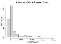
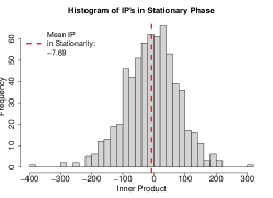
Figure 1: Left panel: Histogram of the inner product of successive gradients (Eq.Β (4)) for SGDM in the transient phase. Right panel: Histogram of the inner products for SGDM in the stationary phase. Training settings from the low β𝛽\beta quadratic setting in SectionΒ III-C. Note the asymmetry in the distribution of inner products in the stationary phase.

Refer to caption Refer to caption

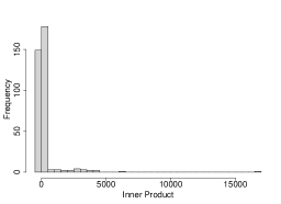
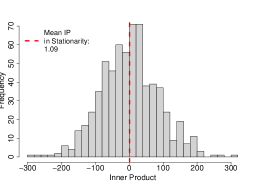
Figure 2: Histogram of the inner product of successive gradients with high momentum Ξ²=0.8𝛽0.8\beta=0.8 and no momentum reduction. Left panel: Transient phase. Right panel: Stationary phase. Quadratic loss model from SectionΒ III-C. Note the symmetry in the distribution of inner products in the stationary phase.

We first provide empirical evidence to support PropositionΒ 6. The low β𝛽\beta quadratic setting from SectionΒ III-C is used, and SGDM run for 20 epochs. In Fig.Β 1 are histograms of the inner products from Eq.Β (4) in the transient and stationary phase. The phase transition is chosen by monitoring MSE with respect to θ⋆subscriptπœƒβ‹†\theta_{\star}. These results have been observed to be robust across loss functions and parameter settings. In the transient phase the inner products are majority positive and have positive skew. This makes sense as when ΞΈnsubscriptπœƒπ‘›\theta_{n} is far away from θ⋆subscriptπœƒβ‹†\theta_{\star}, the bias dominates and gradients are likely pointed in the same direction. In the stationary phase we observe a unimodal distribution around zero with a longer negative tail. What is interesting is the distribution of inner products in the stationary phase. The expectation is negative, and consistently so across many experiments. But the magnitude of the variance exceeds the magnitude of the mean by an order of magnitude. The high magnitude variance indicates a high frequency of iterates with mean zero inner product. The larger negative tail–specifically the small number of inner products around βˆ’400400-400–supports the existence of a small number of key iterates as stated in PropositionΒ 6. This empirical observation is even more striking when you compare similar histograms when the momentum is high Ξ²=0.8𝛽0.8\beta=0.8 and keeping all other settings the same, in Fig.Β 2. The previously observed asymmetry in the stationary phase is now gone. Thus with high momentum (or without momentum reduction), the convergence diagnostic cannot work as there is no clear signal from the test statistic.
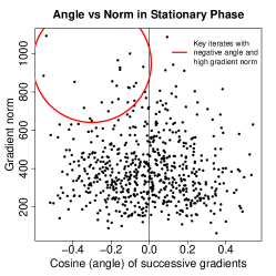
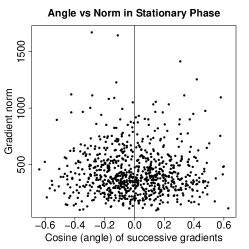
Refer to caption Refer to caption

Figure 3: Cosine similarity vs gradient norm for SGDM in the stationary phase. The red circle indicates those key inner products with negative angle and high gradient norm. Left panel: Training settings from the low β𝛽\beta quadratic setting in SectionΒ III-C. Right panel: high momentum Ξ²=0.8𝛽0.8\beta=0.8. The inner product distribution is symmetric in this case.

Fig.Β 3 provides the further empirical evidence by plotting the magnitude β€–βˆ‡β„“β€‹(ΞΈn,ΞΎn+1)β€–22superscriptsubscriptnormβˆ‡β„“subscriptπœƒπ‘›subscriptπœ‰π‘›122\|\nabla\ell(\theta_{n},\xi_{n+1})\|_{2}^{2} and cosine(βˆ‡β„“β€‹(ΞΈn,ΞΎn+1),βˆ‡β„“β€‹(ΞΈnβˆ’1,ΞΎn))βˆ‡β„“subscriptπœƒπ‘›subscriptπœ‰π‘›1βˆ‡β„“subscriptπœƒπ‘›1subscriptπœ‰π‘›(\nabla\ell(\theta_{n},\xi_{n+1}),\nabla\ell(\theta_{n-1},\xi_{n})) of successive gradients for SGDM in the stationary phase. Again, we first look at the low β𝛽\beta quadratic setting in SectionΒ III-C. A red circle is drawn to identify iterates with high magnitude and negative angle, exactly those key iterates described in PropositionΒ 6. We see such key iterates exist and drive the expectation negative. These results have been observed to be robust across loss functions and parameter settings. With high momentum we have empirically observed that these key inner products with high magnitude and negative angle disappear.

Thus PropositionΒ 6 helps explain the observed sensitivity of the expected test statistic to high momentum.

IV-A Variance bounds

We now provide theory which supports PropositionΒ 6. We show that in the stationary phase, the magnitude of the variance dominates the magnitude of the mean for the test statistic of the convergence diagnostic. A relatively large variance of the inner products βˆ‡β„“β€‹(ΞΈn,ΞΎn+1)βŠ€β€‹βˆ‡β„“β€‹(ΞΈnβˆ’1,ΞΎn)βˆ‡β„“superscriptsubscriptπœƒπ‘›subscriptπœ‰π‘›1topβˆ‡β„“subscriptπœƒπ‘›1subscriptπœ‰π‘›\nabla\ell(\theta_{n},\xi_{n+1})^{\top}\nabla\ell(\theta_{n-1},\xi_{n}) suggests that a majority of iterates are dominated by the variance of the stochastic gradient. A relatively small mean for the inner products suggests that a minority of iterates drive the expectation. Even though in the stationary phase SGDM is trapped in a bounded region, and the expected test statistic driven by a sparse number of key iterates, there is still significant room for random motion.

Theorem 7.

Consider the SGDM procedure in Eq.Β (3). Suppose that AssumptionsΒ 1,Β 2,Β 3,Β 4, andΒ 5 hold. Define
I​P=βˆ‡β„“β€‹(ΞΈn,ΞΎn+1)βŠ€β€‹βˆ‡β„“β€‹(ΞΈnβˆ’1,ΞΎn)πΌπ‘ƒβˆ‡β„“superscriptsubscriptπœƒπ‘›subscriptπœ‰π‘›1topβˆ‡β„“subscriptπœƒπ‘›1subscriptπœ‰π‘›IP=\nabla\ell(\theta_{n},\xi_{n+1})^{\top}\nabla\ell(\theta_{n-1},\xi_{n}). Then,

V​a​r​[I​P]𝔼​[I​P]2π‘‰π‘Žπ‘Ÿdelimited-[]𝐼𝑃𝔼superscriptdelimited-[]𝐼𝑃2\displaystyle\frac{Var[IP]}{\mathbb{E}[IP]^{2}} β‰₯(Mβˆ’L​γ​σ02​AΞ²)2M2​(1+8​L/c)2βˆ’1.β–‘\displaystyle\geq\frac{(M-L\gamma\sigma_{0}^{2}A_{\beta})^{2}}{M^{2}(1+8L/c)^{2}}-1.\hskip 72.26999pt\Box

Corollary 8.

Consider the SGDM procedure in Eq.Β (3). Fix a scaling factor Ξ»>2πœ†2\lambda>2. Set the learning rate Ξ³=2​t​M/L​σ02​Aβ𝛾2𝑑𝑀𝐿superscriptsubscript𝜎02subscript𝐴𝛽\gamma=2tM/L\sigma_{0}^{2}A_{\beta} with tβ‰₯1+λ​(1+4​L/c)𝑑1πœ†14𝐿𝑐t\geq 1+\sqrt{\lambda}(1+4L/c). Then,

Var[IP]β‰₯(Ξ»βˆ’1)𝔼[IP]2.β–‘\hskip 36.135ptVar[IP]\geq(\lambda-1)\ \mathbb{E}[IP]^{2}.\hskip 86.72377pt\Box

Remarks. The results hold regardless of the sign of the expectation of inner products, and show that the variance of the test statistic upper bounds the squared mean. CorollaryΒ 8 specifies that a greater learning rate increases the variance bound. This makes sense as a larger learning rate increases the radius of the stationary region.

We have seen that TheoremΒ 7 and CorollaryΒ 8, along with FiguresΒ 1, 2 andΒ 3, provide theoretical and empirical support for PropositionΒ 6. While the bound in TheoremΒ 7 is more robust to β𝛽\beta, it is still unable to provide practical guidance as the data dependent constants M𝑀M, L𝐿L, c𝑐c, Οƒ02superscriptsubscript𝜎02\sigma_{0}^{2}, and AΞ²subscript𝐴𝛽A_{\beta} must still be estimated.

The convergence diagnostic monitors a certain signal in the gradients. In SectionΒ III we have shown that this signal can be sensitive to high momentum, and in this Section we have shown that the signal may be sparse within other gradient noise. Currently, we believe that an empirical mean is still the best way to capture this gradient signal, with the simple but effective automatic reduction in Alg.Β 1 to combat the negative effects of high momentum.

V Numerical experiments

We now evaluate the convergence diagnostic in Alg.Β 1 on synthetic data experiments in settings of quadratic loss and phase retrievalΒ [9]. The quadratic loss setting is described in SectionΒ III-C. For phase retrieval let ℓ​(ΞΈ,y,x)=1/4​[(xβŠ€β€‹ΞΈ)2βˆ’y]2β„“πœƒπ‘¦π‘₯14superscriptdelimited-[]superscriptsuperscriptπ‘₯topπœƒ2𝑦2\ell(\theta,y,x)=1/4[(x^{\top}\theta)^{2}-y]^{2} with x∼N​(0,I20)similar-toπ‘₯𝑁0subscript𝐼20x\sim N(0,I_{20}) and y=(xβŠ€β€‹ΞΈβ‹†)2𝑦superscriptsuperscriptπ‘₯topsubscriptπœƒβ‹†2y=(x^{\top}\theta_{\star})^{2}. θ⋆,i=(βˆ’1)iΓ—2​exp⁑(βˆ’0.7​i)subscriptπœƒβ‹†π‘–superscript1𝑖20.7𝑖\theta_{\star,i}=(-1)^{i}\times 2\exp(-0.7i) for i=1,…,20𝑖1…20i=1,\dots,20. The number of data points N=103𝑁superscript103N=10^{3}. The checking period c𝑐c is every epoch. Due to non-convexity in phase retrieval we only record the training runs where SGDM has entered a good minima to eliminate the need to tune the parameters for our error rate procedure for different minima.

There are two failure modes: the convergence diagnostic can activate too early, or too late. Let ΞΈnsubscriptπœƒπ‘›\theta_{n} be the estimate when the convergence diagnostic has activated. If the diagnostic activates too early then the error is too high, i.e., β€–ΞΈnβˆ’ΞΈβ‹†β€–2>Ξ·superscriptnormsubscriptπœƒπ‘›subscriptπœƒβ‹†2πœ‚\|\theta_{n}-\theta_{\star}\|^{2}>\eta for some threshold value. Ξ·πœ‚\eta is set as a tight upper bound on the error observed in the stationary phase across many runs. If the diagnostic activates too late, it can waste unnecessary computation. Let K=(nβˆ’k)/nπΎπ‘›π‘˜π‘›K=(n-k)/n such that β€–ΞΈkβˆ’ΞΈnβ€–2=Ξ·superscriptnormsubscriptπœƒπ‘˜subscriptπœƒπ‘›2πœ‚\|\theta_{k}-\theta_{n}\|^{2}=\eta and k≀nπ‘˜π‘›k\leq n. If the diagnostic activates too late, then we expect ΞΈnsubscriptπœƒπ‘›\theta_{n} to be far into the stationary phase, and thus nβˆ’kπ‘›π‘˜n-k to be a significant portion of n𝑛n, i.e., K>ΞΊπΎπœ…K>\kappa for some threshold value. ΞΊπœ…\kappa is set as a tight lower bound on the K𝐾K calculated by running SGDM into the stationary phase.

TableΒ II displays the results of 100 independent runs with the percentage of type I errors (too early), type II errors (too late), and good diagnostic activations. Low and high momentum settings are used for quadratic loss and phase retrieval. Empirically the type I errors are small, while the type II errors are a larger concern. This observation on the higher frequency of type II errors is corroborated byΒ [7]. Encouragingly we see that the automatic momentum reduction in Alg.Β 1 has enabled the convergence diagnostic to be robust to momentum. High momentum settings have little to no effect on the Type I and II error rates of the convergence diagnostic. Contrast TableΒ II with the results in TableΒ I, where the sign of the test statistic in the stationary phase was shown to be sensitive to momentum. Additionally, in approximately 505050-70%percent7070\% of all Type II errors the diagnostic activated only moderately late. In approximately 101010-20%percent2020\% of Type II errors the diagnosticΒ activatedΒ late.

TABLE II: Empirical evaluation of the convergence diagnostic in Alg.Β 1 over 100 independent runs for each experimental setting. SGDM run for 202020 epochs with batch size 202020. Quadratic low β𝛽\beta (Q-Low) set Ξ²=0.2𝛽0.2\beta=0.2, Ξ³=10βˆ’2𝛾superscript102\gamma=10^{-2}, Ξ·=10βˆ’3πœ‚superscript103\eta=10^{-3}, ΞΊ=0.65πœ…0.65\kappa=0.65. Quadratic high β𝛽\beta (Q-High) set Ξ²=0.8𝛽0.8\beta=0.8, Ξ³=10βˆ’2𝛾superscript102\gamma=10^{-2}, Ξ·=2Γ—10βˆ’3πœ‚2superscript103\eta=2\times 10^{-3}, ΞΊ=0.30πœ…0.30\kappa=0.30. Phase retrieval low β𝛽\beta (PR-Low) set Ξ²=0.2𝛽0.2\beta=0.2, Ξ³=10βˆ’2𝛾superscript102\gamma=10^{-2}, Ξ·=10βˆ’2πœ‚superscript102\eta=10^{-2}, ΞΊ=0.6πœ…0.6\kappa=0.6. Phase retrieval high β𝛽\beta (PR-High) set Ξ²=0.8𝛽0.8\beta=0.8, Ξ³=10βˆ’2𝛾superscript102\gamma=10^{-2}, Ξ·=10βˆ’2πœ‚superscript102\eta=10^{-2}, ΞΊ=0.65πœ…0.65\kappa=0.65.
Type I Type II Good
(too early) (too late) activation
Q-Low 1% 22% 77%
Q-High 0% 17% 83%
PR-Low 1% 17% 82%
PR-High 0% 16% 84%

VI Application: an automatic learning rate schedule

The convergence diagnostic has a natural application in automating the learning rate schedule. Hyper-parameter tuning, especially for the learning rate, has a major effect on the performance of stochastic gradient methods. Tuning is typically a very manual process requiring many training re-runs. The benefit of an automatic learning rate is to greatly reduce the amount of supervision and number of training runs.

input :Β Alg.Β 1 SGDM(ΞΈ,Ξ³)πœƒπ›Ύ(\theta,\gamma), initial and minimum stepsize Ξ³0subscript𝛾0\gamma_{0}, Ξ³m​i​nsubscriptπ›Ύπ‘šπ‘–π‘›\gamma_{min}, learning rate reduction ρ∈(0,1)𝜌01\rho\in(0,1)
1 γ←γ0←𝛾subscript𝛾0\gamma\leftarrow\gamma_{0}
2 whileΒ Ξ³>Ξ³m​i​n𝛾subscriptπ›Ύπ‘šπ‘–π‘›\gamma>\gamma_{min}Β do
3Β Β Β Β Β Β  ΞΈβ†πš‚π™Άπ™³π™Όβ€‹(ΞΈ,Ξ³)β†πœƒπš‚π™Άπ™³π™Όπœƒπ›Ύ\theta\leftarrow{\tt SGDM}(\theta,\gamma)
4Β Β Β Β Β Β  Ξ³β†ΟΓ—Ξ³β†π›ΎπœŒπ›Ύ\gamma\leftarrow\rho\times\gamma
5Β Β Β Β Β Β 
6 end while
return ΞΈπœƒ\theta
AlgorithmΒ 2 SGDM with automatic learning rate

In Alg.Β 2 we present an automatic learning rate based on the convergence diagnostic in Alg.Β 1. SGDM with constant learning rate moves quickly towards θ⋆subscriptπœƒβ‹†\theta_{\star} but cannot improve beyond distance O​(Ξ³)𝑂𝛾O(\gamma), as suggested by TheoremΒ 1. The convergence diagnostic is used to detect stationarity, after which the learning rate is reduced Ξ³β†Οβ€‹Ξ³β†π›ΎπœŒπ›Ύ\gamma\leftarrow\rho\gamma and a smaller radius O​(ρ​γ)π‘‚πœŒπ›ΎO(\rho\gamma) of stationarity achieved, with ρ∈(0,1)𝜌01\rho\in(0,1). Alg.Β 2 takes advantage of the speedup afforded to constant rate in the transient phase, while avoiding the trade-off cost of a larger stationary region by reducing the learning rate. In practice it is common to use a constant learning rate and decrease several times at hand chosen pointsΒ [13, 17].

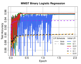
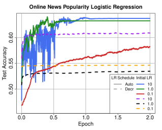
A major benefit of automatic hyper-parameter tuning is robustness to a potentially misspecified initial setting, in this case Ξ³0subscript𝛾0\gamma_{0}. We train logistic regression on benchmark datasets MNIST and Online News Popularity (from UCI repository), for a variety of initial learning rates Ξ³0subscript𝛾0\gamma_{0}. In Fig.Β 4 the accuracy on a held out test set is compared between the automatic rate in Alg.Β 2 and a decreasing rate Ξ³=Ξ³0/n𝛾subscript𝛾0𝑛\gamma=\gamma_{0}/n for Ξ³0m​n​i​s​t∈{1.0,0.1,0.01}superscriptsubscript𝛾0π‘šπ‘›π‘–π‘ π‘‘1.00.10.01\gamma_{0}^{mnist}\in\{1.0,0.1,0.01\} in MNIST and Ξ³0n​e​w​s∈{10,1.0,0.1}superscriptsubscript𝛾0𝑛𝑒𝑀𝑠101.00.1\gamma_{0}^{news}\in\{10,1.0,0.1\} in Online News. The findings are consistent across both datasets. The automatic learning rate was significantly more robust to initial conditions than the decreasing rate. In addition, the automatic learning rate achieved significantly higher test accuracy than theΒ decreasingΒ rate.

Refer to caption
Refer to caption
Figure 4: Binary logistic regression with SGDM using Alg.Β 2 and decreasing rate Ξ³=Ξ³0/n𝛾subscript𝛾0𝑛\gamma=\gamma_{0}/n, Ξ²=0.8𝛽0.8\beta=0.8. Upper panel: MNIST. Bottom panel: Online News Popularity.
Refer to caption
Refer to caption
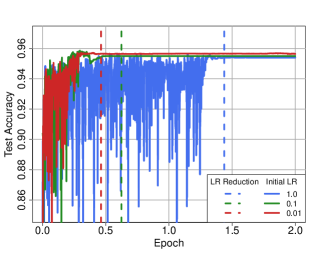
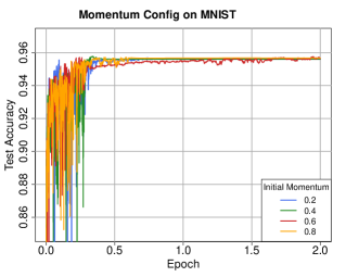
Figure 5: Upper: Vertical lines marks the diagnostic activation and learning rate reduction on MNIST. Bottom: SGDM using Alg.Β 2 and varying momentum β∈{0.2,0.4,0.6,0.8}𝛽0.20.40.60.8\beta\in\{0.2,0.4,0.6,0.8\}.

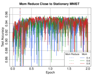
In Fig.Β 5 (upper panel) we plot only SGDM using Alg.Β 2 and vertical lines to mark the convergence diagnostic’s activation. On the bottom panel of Fig.Β 5 shows SGDM using Alg.Β 2 with varying initial momentum. From the similarity in training curves we see that Alg.Β 2 is also robust to setting the momentum. The function h​()β„Žh() we used in Alg.Β 1 to set the change in momentum was the mean squared distance between successive iterates. However, any convergence heuristic can be used for h​()β„Žh() in Alg.Β 1. We show that h​()β„Žh() works consistently in the upper panel of Fig.Β 6. Regardless of the initial momentum, SGDM using Alg.Β 2 on MNIST reduces the initial momentum at a consistent point, helping to ensure a consistent activation of the convergence diagnostic.
Refer to caption
Refer to caption
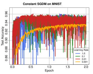
Figure 6: Upper: Vertical line marks a consistent momentum reduction using convergence heuristic of β€–ΞΈnβˆ’ΞΈnβˆ’1β€–2superscriptnormsubscriptπœƒπ‘›subscriptπœƒπ‘›12\|\theta_{n}-\theta_{n-1}\|^{2}. Bottom: Binary logistic regression with SGDM using Alg.Β 2 and constant learning rate Ξ³0∈{1.0,0.1,0.01,0.001}subscript𝛾01.00.10.010.001\gamma_{0}\in\{1.0,0.1,0.01,0.001\} on MNIST.

Experiments were performed with constant rate Ξ³=Ξ³0𝛾subscript𝛾0\gamma=\gamma_{0}, however the stationary region was large enough to result in significant test accuracy fluctuations for a given Ξ³0subscript𝛾0\gamma_{0}.

Refer to caption
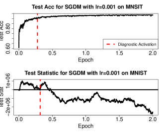
Figure 7: Test accuracy and convergence diagnostic test statistic from Alg.Β 1 on MNIST. The vertical line marks the diagnostic’s activation, which coincides with the test accuracy flattening out.

The fact that SGDM using Alg.Β 2 is able to achieve competitive performance indicates that the convergence diagnostic is working well. As further evidence that the convergence diagnostic in Alg.Β 1 is working well, Fig.Β 7 plots the test statistic of the convergence diagnostic along with the test accuracy for SGDM on MNIST. The vertical line indicates the activation of the convergence diagnostic, when the test statistic becomes negative. The diagnostic activates just as the test accuracy flattens out.
Refer to caption
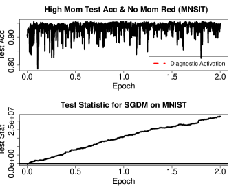
Figure 8: Test accuracy and convergence diagnostic test statistic on MNIST. The momentum reduction has been removed, and Ξ²=0.8𝛽0.8\beta=0.8. The test accuracy has flattened out and SGDM has converged, but the diagnostic does not activate because the test statistic is perpetually positive.

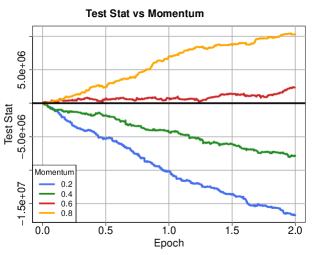
We conduct an ablation study to understand the negative effects of high momentum on our convergence diagnostic. Fig.Β 8 plots the test accuracy and test statistic by removing the momentum reduction component of Alg.Β 1 and using SGDM with high momentum Ξ²=0.8𝛽0.8\beta=0.8 on MNIST. SGDM has convergence because the test accuracy has plateaued, but the convergence diagnostic does not activate because its test statistic is perpetually positive. We plot the test statistic of Alg.Β 1 in Fig.Β 9 with no momentum reduction and increasing momentum β∈{0.2,0.4,0.6,0.8}𝛽0.20.40.60.8\beta\in\{0.2,0.4,0.6,0.8\}. Momentum has a proportional relationship with the slope of the test statistic. A positive slope indicates that the test statistic is not negative upon convergence, and thus the convergence diagnostic without the momentum reduction is ineffective for higher momentum β∈{0.6,0.8}𝛽0.60.8\beta\in\{0.6,0.8\} on MNIST.

Refer to caption
Figure 9: Test statistic for different values of momentum β∈{0.2,0.4,0.6,0.8}𝛽0.20.40.60.8\beta\in\{0.2,0.4,0.6,0.8\}. Higher momentum increases the slope of the test statistic, indicating an even greater difficulty for the convergence diagnostic to detect the stationary phase.

VII Conclusion

In this paper we focus on detecting the phase transition of SGDM (stochastic gradient descent with momentum) to the stationary phase. Inspiration is drawn from literature on stopping times in stochastic approximation. Momentum introduces challenges in the construction and operation of the test statistic for the convergence diagnostic. We present theory and experiments which support that high momentum alters the trajectory of the stochastic gradients which the diagnostic monitors. In addition we show the dynamics of SGDM in stationarity are largely random with a sparse number of key iterates behaving in an informative way, which the diagnostic is able to capture. The proposed automatic momentum reduction technique resolves the issues with high momentum. Empirical results demonstrate that the diagnostic has few type I errors and a reasonably small number of type II errors, and thus reliably detects convergence to the stationary phase. We present an application to an automatic learning rate and show that it is robust to initial conditions.

Future work include extensions to other stochastic gradient methods such as adaptive gradient or distributed methods such as β€œlocal method” [8] are of great interest.

References

  • [1] FrancisΒ R. Bach and Eric Moulines. Non-asymptotic analysis of stochastic approximation algorithms for machine learning. In Advances in Neural Information Processing Systems (NIPS), pages 451–459, Granada, Spain, 2011.
  • [2] FrancisΒ R. Bach and Eric Moulines. Non-strongly-convex smooth stochastic approximation with convergence rate O(1/n). In Advances in Neural Information Processing Systems (NIPS), pages 773–781, Lake Tahoe, NV, 2013.
  • [3] Avrim Blum, Adam Kalai, and John Langford. Beating the hold-out: Bounds for k-fold and progressive cross-validation. In Shai Ben-David and PhilipΒ M. Long, editors, Proceedings of the Twelfth Annual Conference on Computational Learning Theory (COLT), pages 203–208, Santa Cruz, CA, 1999.
  • [4] LΓ©on Bottou. Large-scale machine learning with stochastic gradient descent. In Yves Lechevallier and Gilbert Saporta, editors, Proceedings of the 19th International Conference on Computational Statistics (COMPSTAT), pages 177–186, Paris, France, 2010.
  • [5] LΓ©on Bottou. Stochastic gradient descent tricks. In GrΓ©goire Montavon, GenevieveΒ B. Orr, and Klaus-Robert MΓΌller, editors, Neural Networks: Tricks of the Trade - Second Edition, volume 7700 of Lecture Notes in Computer Science, pages 421–436. Springer, 2012.
  • [6] LΓ©on Bottou, FrankΒ E. Curtis, and Jorge Nocedal. Optimization methods for large-scale machine learning. SIAM Review, 60(2):223–311, 2018.
  • [7] Jerry Chee and Panos Toulis. Convergence diagnostics for stochastic gradient descent with constant learning rate. In International Conference on Artificial Intelligence and Statistics (AISTATS), pages 1476–1485, Playa Blanca, Lanzarote, Canary Islands, Spain, 2018.
  • [8] Xiangyi Chen, Xiaoyun Li, and Ping Li. Toward communication efficient adaptive gradient method. In ACM-IMS Foundations of Data Science Conference (FODS), Seattle, WA, 2020.
  • [9] Yuxin Chen, Yuejie Chi, Jianqing Fan, and Cong Ma. Gradient descent with random initialization: fast global convergence for nonconvex phase retrieval. Math. Program., 176(1-2):5–37, 2019.
  • [10] Bernard Delyon and AnatoliΒ B. Juditsky. Accelerated stochastic approximation. SIAM Journal on Optimization, 3(4):868–881, 1993.
  • [11] YuΒ M Ermoliev and RJ-B Wets. Numerical techniques for stochastic optimization. Springer-Verlag, 1988.
  • [12] Rong Ge, ShamΒ M. Kakade, Rahul Kidambi, and Praneeth Netrapalli. The step decay schedule: A near optimal, geometrically decaying learning rate procedure for least squares. In Advances in Neural Information Processing Systems (NeurIPS), pages 14951–14962, Vancouver, Canada, 2019.
  • [13] Kaiming He, Xiangyu Zhang, Shaoqing Ren, and Jian Sun. Deep residual learning for image recognition. In Proceedings of the 2016 IEEE Conference on Computer Vision and Pattern Recognition (CVPR), pages 770–778, Las Vegas, NV, 2016.
  • [14] NitishΒ Shirish Keskar and Richard Socher. Improving generalization performance by switching from adam to SGD. Technical report, arXiv:1712.07628, 2017.
  • [15] Harry Kesten. Accelerated stochastic approximation. The Annals of Mathematical Statistics, 29(1):41–59, 1958.
  • [16] DiederikΒ P. Kingma and Jimmy Ba. Adam: A method for stochastic optimization. In Proceedings of the 3rd International Conference on Learning Representations (ICLR), San Diego, CA, 2015.
  • [17] Alex Krizhevsky, Ilya Sutskever, and GeoffreyΒ E. Hinton. Imagenet classification with deep convolutional neural networks. Commun. ACM, 60(6):84–90, 2017.
  • [18] Hunter Lang, Lin Xiao, and Pengchuan Zhang. Using statistics to automate stochastic optimization. In Advances in Neural Information Processing Systems (NeurIPS), pages 9536–9546, Vancouver, Canada, 2019.
  • [19] Nicolas Loizou and Peter RichtΓ‘rik. Momentum and stochastic momentum for stochastic gradient, newton, proximal point and subspace descent methods. Technical report, arXiv:1712.09677, 2017.
  • [20] Noboru Murata. A statistical study of on-line learning. Online Learning and Neural Networks. Cambridge University Press, Cambridge, UK, pages 63–92, 1998.
  • [21] Deanna Needell, Nathan Srebro, and Rachel Ward. Stochastic gradient descent, weighted sampling, and the randomized kaczmarz algorithm. Math. Program., 155(1-2):549–573, 2016.
  • [22] Arkadi Nemirovski, AnatoliΒ B. Juditsky, Guanghui Lan, and Alexander Shapiro. Robust stochastic approximation approach to stochastic programming. SIAM Journal on Optimization, 19(4):1574–1609, 2009.
  • [23] GeorgΒ Ch Pflug. Non-asymptotic confidence bounds for stochastic approximation algorithms with constant step size. Monatshefte fΓΌr Mathematik, 110(3):297–314, 1990.
  • [24] B.T. Polyak. Some methods of speeding up the convergence of iteration methods. USSR Computational Mathematics and Mathematical Physics, 4(5):1–17, 1964.
  • [25] SashankΒ J. Reddi, Ahmed Hefny, Suvrit Sra, BarnabΓ‘s PΓ³czos, and AlexanderΒ J. Smola. On variance reduction in stochastic gradient descent and its asynchronous variants. In Corinna Cortes, NeilΒ D. Lawrence, DanielΒ D. Lee, Masashi Sugiyama, and Roman Garnett, editors, Advances in Neural Information Processing Systems (NIPS), pages 2647–2655, Montreal, Canada, 2015.
  • [26] NicolasΒ Le Roux, Mark Schmidt, and FrancisΒ R. Bach. A stochastic gradient method with an exponential convergence rate for finite training sets. In Advances in Neural Information Processing Systems (NIPS), pages 2672–2680, Lake Tahoe, NV, 2012.
  • [27] Matteo Sordello and Weijie Su. Data-adaptive learning rate selection for stochastic gradient descent using convergence diagnostic. Joint Statistics Meeting, 2019.
  • [28] Weijie Su and Yuancheng Zhu. Uncertainty quantification for online learning and stochastic approximation via hierarchical incremental gradient descent. Technical report, arXiv:1802.04876, 2018.
  • [29] ZheΒ Li TianbaoΒ Yang, QihangΒ Lin. Unified convergence analysis of stochastic momentum methods for convex and non-convex optimization. Technical report, arXiv:1604.03257, 2016.
  • [30] Panos Toulis and EdoardoΒ M. Airoldi. Scalable estimation strategies based on stochastic approximations: classical results and new insights. Stat. Comput., 25(4):781–795, 2015.
  • [31] Panos Toulis, EdoardoΒ M Airoldi, etΒ al. Asymptotic and finite-sample properties of estimators based on stochastic gradients. The Annals of Statistics, 45(4):1694–1727, 2017.
  • [32] Sho Yaida. Fluctuation-dissipation relations for stochastic gradient descent. In Proceedings of the 7th International Conference on Learning Representations (ICLR), New Orleans, LA, 2019.
  • [33] George Yin. Stopping times for stochastic approximation. In Modern Optimal Control: A Conference in Honor of Solomon Lefschetz and Joseph P. LaSalle, pages 409–420, 1989.
  • [34] Tong Zhang. Solving large scale linear prediction problems using stochastic gradient descent algorithms. In Proceedings of the Twenty-first International Conference on Machine Learning (ICML), Banff, Canada, 2004.

VIII Proofs for SectionΒ III

We re-state the assumptions:

Assumption 1. Β The expected loss f​(ΞΈ)=𝔼​[ℓ​(ΞΈ,ΞΎ)]π‘“πœƒπ”Όdelimited-[]β„“πœƒπœ‰f(\theta)=\mathbb{E}[\ell(\theta,\xi)] is strongly convex with constant c𝑐c.

Assumption 2. Β The expected loss f​(ΞΈ)=𝔼​[ℓ​(ΞΈ,ΞΎ)]π‘“πœƒπ”Όdelimited-[]β„“πœƒπœ‰f(\theta)=\mathbb{E}[\ell(\theta,\xi)] is Lipschitz-smooth with constant L𝐿L.

Assumption 3. Β TheoremΒ 1Β [29] holds s.t. 𝔼​[f​(ΞΈn)βˆ’f​(θ⋆)]≀γ​M𝔼delimited-[]𝑓subscriptπœƒπ‘›π‘“subscriptπœƒβ‹†π›Ύπ‘€\mathbb{E}[f(\theta_{n})-f(\theta_{\star})]\leq\gamma M for some M>0𝑀0M>0 and large enough n𝑛n.

Assumption 4. Β βˆƒΟƒ02>0superscriptsubscript𝜎020\exists\ \sigma_{0}^{2}>0 s.t. 𝔼​[β€–βˆ‡β„“β€‹(ΞΈ,ΞΎ)β€–2]>Οƒ02𝔼delimited-[]superscriptnormβˆ‡β„“πœƒπœ‰2superscriptsubscript𝜎02\mathbb{E}[\|\nabla\ell(\theta,\xi)\|^{2}]>\sigma_{0}^{2}.

Assumption 5. Β βˆƒK>1𝐾1\exists\ K>1 s.t. 𝔼​[(ΞΈnβˆ’ΞΈnβˆ’1)βŠ€β€‹(ΞΈnβˆ’1βˆ’ΞΈnβˆ’2)]β‰₯βˆ’K​𝔼​[β€–ΞΈnβˆ’ΞΈnβˆ’1β€–2]𝔼delimited-[]superscriptsubscriptπœƒπ‘›subscriptπœƒπ‘›1topsubscriptπœƒπ‘›1subscriptπœƒπ‘›2𝐾𝔼delimited-[]superscriptnormsubscriptπœƒπ‘›subscriptπœƒπ‘›12\mathbb{E}[(\theta_{n}-\theta_{n-1})^{\top}(\theta_{n-1}-\theta_{n-2})]\geq-K\mathbb{E}[\|\theta_{n}-\theta_{n-1}\|^{2}] for large enough n𝑛n.

Firstly, we derive a lower bound on the expected distance between iterates.

Lemma 9.

Suppose that AssumptionsΒ 4 andΒ 5 hold. Then for large enough n𝑛n,

𝔼​[β€–ΞΈnβˆ’ΞΈnβˆ’1β€–2]β‰₯Ξ³2​σ02​(11+2​K​β+Ξ²2)𝔼delimited-[]superscriptnormsubscriptπœƒπ‘›subscriptπœƒπ‘›12superscript𝛾2superscriptsubscript𝜎02112𝐾𝛽superscript𝛽2\mathbb{E}[\|\theta_{n}-\theta_{n-1}\|^{2}]\geq\gamma^{2}\sigma_{0}^{2}\biggl{(}\frac{1}{1+2K\beta+\beta^{2}}\biggr{)}
Proof.

By re-arranging the update equation for SGDM in Eq.Β (3), we get ΞΈnβˆ’ΞΈnβˆ’1βˆ’Ξ²β€‹(ΞΈnβˆ’1βˆ’ΞΈnβˆ’2)=βˆ’Ξ³β€‹βˆ‡β„“β€‹(ΞΈnβˆ’1,ΞΎn)subscriptπœƒπ‘›subscriptπœƒπ‘›1𝛽subscriptπœƒπ‘›1subscriptπœƒπ‘›2π›Ύβˆ‡β„“subscriptπœƒπ‘›1subscriptπœ‰π‘›\theta_{n}-\theta_{n-1}-\beta(\theta_{n-1}-\theta_{n-2})=-\gamma\nabla\ell(\theta_{n-1},\xi_{n}). For brevity, let Ξ”n≑θnβˆ’ΞΈnβˆ’1subscriptΔ𝑛subscriptπœƒπ‘›subscriptπœƒπ‘›1\Delta_{n}\equiv\theta_{n}-\theta_{n-1}, and βˆ‡β„“nβ‰‘βˆ‡β„“β€‹(ΞΈnβˆ’1,ΞΎn)βˆ‡subscriptβ„“π‘›βˆ‡β„“subscriptπœƒπ‘›1subscriptπœ‰π‘›\nabla\ell_{n}\equiv\nabla\ell(\theta_{n-1},\xi_{n}). Applying squared norm and re-arranging terms,

β€–Ξ”nβˆ’Ξ²β€‹Ξ”nβˆ’1β€–2superscriptnormsubscriptΔ𝑛𝛽subscriptΔ𝑛12\displaystyle\|\Delta_{n}-\beta\Delta_{n-1}\|^{2} =β€–βˆ’Ξ³β€‹βˆ‡β„“nβ€–2absentsuperscriptnormπ›Ύβˆ‡subscriptℓ𝑛2\displaystyle=\|-\gamma\nabla\ell_{n}\|^{2}
β€–Ξ”nβ€–2superscriptnormsubscriptΔ𝑛2\displaystyle\|\Delta_{n}\|^{2} =Ξ³2β€‹β€–βˆ‡β„“nβ€–2+2​β​ΔnβŠ€β€‹Ξ”nβˆ’1βˆ’Ξ²2​‖Δnβˆ’1β€–2absentsuperscript𝛾2superscriptnormβˆ‡subscriptℓ𝑛22𝛽superscriptsubscriptΔ𝑛topsubscriptΔ𝑛1superscript𝛽2superscriptnormsubscriptΔ𝑛12\displaystyle=\gamma^{2}\|\nabla\ell_{n}\|^{2}+2\beta\Delta_{n}^{\top}\Delta_{n-1}-\beta^{2}\|\Delta_{n-1}\|^{2}

Apply expectations to both sides and the second inequality assumption to define a recursive relation.

𝔼​[β€–Ξ”nβ€–2]𝔼delimited-[]superscriptnormsubscriptΔ𝑛2\displaystyle\mathbb{E}[\|\Delta_{n}\|^{2}] =Ξ³2​𝔼​[β€–βˆ‡β„“nβ€–2]+2​β​𝔼​[Ξ”nβŠ€β€‹Ξ”nβˆ’1]βˆ’Ξ²2​𝔼​[β€–Ξ”nβˆ’1β€–2]absentsuperscript𝛾2𝔼delimited-[]superscriptnormβˆ‡subscriptℓ𝑛22𝛽𝔼delimited-[]superscriptsubscriptΔ𝑛topsubscriptΔ𝑛1superscript𝛽2𝔼delimited-[]superscriptnormsubscriptΔ𝑛12\displaystyle=\gamma^{2}\mathbb{E}[\|\nabla\ell_{n}\|^{2}]+2\beta\mathbb{E}[\Delta_{n}^{\top}\Delta_{n-1}]-\beta^{2}\mathbb{E}[\|\Delta_{n-1}\|^{2}]
β‰₯Ξ³2​σ02βˆ’π”Όβ€‹[β€–Ξ”nβˆ’1β€–2]​(2​β​K+Ξ²2)absentsuperscript𝛾2superscriptsubscript𝜎02𝔼delimited-[]superscriptnormsubscriptΔ𝑛122𝛽𝐾superscript𝛽2\displaystyle\geq\gamma^{2}\sigma_{0}^{2}-\mathbb{E}[\|\Delta_{n-1}\|^{2}](2\beta K+\beta^{2})

Using this recursive relation we obtain

𝔼​[β€–Ξ”nβ€–2]𝔼delimited-[]superscriptnormsubscriptΔ𝑛2\displaystyle\mathbb{E}[\|\Delta_{n}\|^{2}] β‰₯Ξ³2β€‹βˆ‘i=0nβˆ’1(βˆ’1)i​(2​β​K+Ξ²2)i​σ02=Ξ³2​σ02​(1βˆ’(2​β​K+Ξ²2)n1+2​β​K+Ξ²2)absentsuperscript𝛾2superscriptsubscript𝑖0𝑛1superscript1𝑖superscript2𝛽𝐾superscript𝛽2𝑖superscriptsubscript𝜎02superscript𝛾2superscriptsubscript𝜎021superscript2𝛽𝐾superscript𝛽2𝑛12𝛽𝐾superscript𝛽2\displaystyle\geq\gamma^{2}\sum_{i=0}^{n-1}(-1)^{i}(2\beta K+\beta^{2})^{i}\sigma_{0}^{2}=\gamma^{2}\sigma_{0}^{2}\biggl{(}\frac{1-(2\beta K+\beta^{2})^{n}}{1+2\beta K+\beta^{2}}\biggr{)}

Because we expect the number of iterations n𝑛n to be large when entering the stationary phase, we make the approximation

𝔼​[β€–Ξ”nβ€–2]𝔼delimited-[]superscriptnormsubscriptΔ𝑛2\displaystyle\mathbb{E}[\|\Delta_{n}\|^{2}] β‰₯Ξ³2​σ02​(11+2​β​K+Ξ²2)absentsuperscript𝛾2superscriptsubscript𝜎02112𝛽𝐾superscript𝛽2\displaystyle\geq\gamma^{2}\sigma_{0}^{2}\biggl{(}\frac{1}{1+2\beta K+\beta^{2}}\biggr{)}

∎

Remarks. If 𝔼​[Ξ”nβŠ€β€‹Ξ”nβˆ’1]>0𝔼delimited-[]superscriptsubscriptΔ𝑛topsubscriptΔ𝑛10\mathbb{E}[\Delta_{n}^{\top}\Delta_{n-1}]>0 then any negative lower bound is trivial. It is reasonable to assume K𝐾K is not too large. We expect β€–ΞΈnβˆ’ΞΈnβˆ’1β€–2β‰ˆβ€–ΞΈnβˆ’1βˆ’ΞΈnβˆ’2β€–2superscriptnormsubscriptπœƒπ‘›subscriptπœƒπ‘›12superscriptnormsubscriptπœƒπ‘›1subscriptπœƒπ‘›22\|\theta_{n}-\theta_{n-1}\|^{2}\approx\|\theta_{n-1}-\theta_{n-2}\|^{2} because they are successive iterates.

Theorem 2.

Suppose that AssumptionsΒ 1,Β 3, andΒ 4 hold. The test statistic for the convergence diagnostic in AlgorithmΒ 1 for SGDM in Eq.Β (3) is bounded

𝔼​[βˆ‡β„“β€‹(ΞΈn,ΞΎn+1)βŠ€β€‹βˆ‡β„“β€‹(ΞΈnβˆ’1,ΞΎn)]≀(1+Ξ²)​[Mβˆ’c2​γ​σ02​AΞ²]<0𝔼delimited-[]βˆ‡β„“superscriptsubscriptπœƒπ‘›subscriptπœ‰π‘›1topβˆ‡β„“subscriptπœƒπ‘›1subscriptπœ‰π‘›1𝛽delimited-[]𝑀𝑐2𝛾superscriptsubscript𝜎02subscript𝐴𝛽0\mathbb{E}[\nabla\ell(\theta_{n},\xi_{n+1})^{\top}\nabla\ell(\theta_{n-1},\xi_{n})]\leq(1+\beta)\left[M-\frac{c}{2}\gamma\sigma_{0}^{2}A_{\beta}\right]<0

as nβ†’βˆžβ†’π‘›n\rightarrow\infty. And thus the convergence diagnostic activates almost surely.

Proof.

First re-write the inner product with the decomposition in Eq.Β (6).

βˆ‡β„“β€‹(ΞΈn,ΞΎn+1)βŠ€β€‹βˆ‡β„“β€‹(ΞΈnβˆ’1,ΞΎn)βˆ‡β„“superscriptsubscriptπœƒπ‘›subscriptπœ‰π‘›1topβˆ‡β„“subscriptπœƒπ‘›1subscriptπœ‰π‘›\displaystyle\nabla\ell(\theta_{n},\xi_{n+1})^{\top}\nabla\ell(\theta_{n-1},\xi_{n}) =1Ξ³β€‹βˆ‡β„“β€‹(ΞΈn,ΞΎn+1)βŠ€β€‹(ΞΈnβˆ’1βˆ’ΞΈn)+Ξ²Ξ³β€‹βˆ‡β„“β€‹(ΞΈn,ΞΎn+1)βŠ€β€‹(ΞΈnβˆ’1βˆ’ΞΈnβˆ’2)absent1π›Ύβˆ‡β„“superscriptsubscriptπœƒπ‘›subscriptπœ‰π‘›1topsubscriptπœƒπ‘›1subscriptπœƒπ‘›π›½π›Ύβˆ‡β„“superscriptsubscriptπœƒπ‘›subscriptπœ‰π‘›1topsubscriptπœƒπ‘›1subscriptπœƒπ‘›2\displaystyle=\frac{1}{\gamma}\nabla\ell(\theta_{n},\xi_{n+1})^{\top}(\theta_{n-1}-\theta_{n})+\frac{\beta}{\gamma}\nabla\ell(\theta_{n},\xi_{n+1})^{\top}(\theta_{n-1}-\theta_{n-2})

Apply expectation to both sides, and then apply the strong convexity assumption.

𝔼​[βˆ‡β„“β€‹(ΞΈn,ΞΎn+1)βŠ€β€‹βˆ‡β„“β€‹(ΞΈnβˆ’1,ΞΎn)]𝔼delimited-[]βˆ‡β„“superscriptsubscriptπœƒπ‘›subscriptπœ‰π‘›1topβˆ‡β„“subscriptπœƒπ‘›1subscriptπœ‰π‘›\displaystyle\mathbb{E}[\nabla\ell(\theta_{n},\xi_{n+1})^{\top}\nabla\ell(\theta_{n-1},\xi_{n})] ≀1γ​[f​(ΞΈnβˆ’1)βˆ’f​(ΞΈn)βˆ’c2​‖θnβˆ’1βˆ’ΞΈnβ€–2]absent1𝛾delimited-[]𝑓subscriptπœƒπ‘›1𝑓subscriptπœƒπ‘›π‘2superscriptnormsubscriptπœƒπ‘›1subscriptπœƒπ‘›2\displaystyle\leq\frac{1}{\gamma}[f(\theta_{n-1})-f(\theta_{n})-\frac{c}{2}\|\theta_{n-1}-\theta_{n}\|^{2}]
+βγ​[f​(ΞΈnβˆ’1βˆ’ΞΈnβˆ’2+ΞΈn)βˆ’f​(ΞΈn)βˆ’c2​‖θnβˆ’1βˆ’ΞΈnβˆ’2β€–2]𝛽𝛾delimited-[]𝑓subscriptπœƒπ‘›1subscriptπœƒπ‘›2subscriptπœƒπ‘›π‘“subscriptπœƒπ‘›π‘2superscriptnormsubscriptπœƒπ‘›1subscriptπœƒπ‘›22\displaystyle\quad+\frac{\beta}{\gamma}[f(\theta_{n-1}-\theta_{n-2}+\theta_{n})-f(\theta_{n})-\frac{c}{2}\|\theta_{n-1}-\theta_{n-2}\|^{2}]
≀1γ​[f​(ΞΈnβˆ’1)βˆ’f​(θ⋆)βˆ’c2​‖θnβˆ’1βˆ’ΞΈnβ€–2]absent1𝛾delimited-[]𝑓subscriptπœƒπ‘›1𝑓subscriptπœƒβ‹†π‘2superscriptnormsubscriptπœƒπ‘›1subscriptπœƒπ‘›2\displaystyle\leq\frac{1}{\gamma}[f(\theta_{n-1})-f(\theta_{\star})-\frac{c}{2}\|\theta_{n-1}-\theta_{n}\|^{2}]
+βγ​[f​(ΞΈnβˆ’1βˆ’ΞΈnβˆ’2+ΞΈn)βˆ’f​(θ⋆)βˆ’c2​‖θnβˆ’1βˆ’ΞΈnβˆ’2β€–2]𝛽𝛾delimited-[]𝑓subscriptπœƒπ‘›1subscriptπœƒπ‘›2subscriptπœƒπ‘›π‘“subscriptπœƒβ‹†π‘2superscriptnormsubscriptπœƒπ‘›1subscriptπœƒπ‘›22\displaystyle\quad+\frac{\beta}{\gamma}[f(\theta_{n-1}-\theta_{n-2}+\theta_{n})-f(\theta_{\star})-\frac{c}{2}\|\theta_{n-1}-\theta_{n-2}\|^{2}]

Now extend the expectation over randomness in the trajectory, and apply the result from TheoremΒ 1 and LemmaΒ 9.

≀1γ​[γ​Mβˆ’c2​γ2​σ02​AΞ²]+βγ​[γ​Mβˆ’c2​γ2​σ02​AΞ²]absent1𝛾delimited-[]𝛾𝑀𝑐2superscript𝛾2superscriptsubscript𝜎02subscript𝐴𝛽𝛽𝛾delimited-[]𝛾𝑀𝑐2superscript𝛾2superscriptsubscript𝜎02subscript𝐴𝛽\displaystyle\leq\frac{1}{\gamma}\bigg{[}\gamma M-\frac{c}{2}\gamma^{2}\sigma_{0}^{2}A_{\beta}\bigg{]}+\frac{\beta}{\gamma}\bigg{[}\gamma M-\frac{c}{2}\gamma^{2}\sigma_{0}^{2}A_{\beta}\bigg{]}
=(1+Ξ²)​[Mβˆ’c2​γ​σ02​AΞ²]absent1𝛽delimited-[]𝑀𝑐2𝛾superscriptsubscript𝜎02subscript𝐴𝛽\displaystyle=(1+\beta)[M-\frac{c}{2}\gamma\sigma_{0}^{2}A_{\beta}]

∎

Remarks. AΞ²=1/(1+2​β​K+Ξ²2)subscript𝐴𝛽112𝛽𝐾superscript𝛽2A_{\beta}=1/(1+2\beta K+\beta^{2}) from LemmaΒ 9. AΞ²subscript𝐴𝛽A_{\beta} is a monotonically decreasing function, where AΞ²|Ξ²=0=1subscript𝐴conditional𝛽𝛽01A_{\beta|\beta=0}=1, and AΞ²|Ξ²=1=1/(2+2​K)subscript𝐴conditional𝛽𝛽1122𝐾A_{\beta|\beta=1}=1/(2+2K). Thus for the condition on the learning rate, higher β𝛽\beta causes lower AΞ²subscript𝐴𝛽A_{\beta} which increasesΒ theΒ conditionΒ onΒ Ξ³2superscript𝛾2\gamma^{2}.

We now derive bounds similar to TheoremΒ 2 for the alternative test statistic constructed in Eq.Β (5), and show that its expectation is highly sensitive to momentum. This increased sensitivity makes it a poor choice to use in a convergenceΒ diagnostic.

Theorem 3.

Suppose that AssumptionsΒ 1,Β 3, andΒ 4 hold. Then,

𝔼[(βˆ‡β„“(ΞΈn,ΞΎn+1)+Ξ²\displaystyle\mathbb{E}[(\nabla\ell(\theta_{n},\xi_{n+1})+\beta (ΞΈnβˆ’ΞΈnβˆ’1))⊀(βˆ‡β„“(ΞΈnβˆ’1,ΞΎn)+Ξ²(ΞΈnβˆ’1βˆ’ΞΈnβˆ’2))]\displaystyle(\theta_{n}-\theta_{n-1}))^{\top}(\nabla\ell(\theta_{n-1},\xi_{n})+\beta(\theta_{n-1}-\theta_{n-2}))]
<(1Ξ³+Ξ²Ξ³+2​β+Ξ²2)​[γ​Mβˆ’c2​γ2​σ02​AΞ²]+Ξ²3​γ​Mabsent1𝛾𝛽𝛾2𝛽superscript𝛽2delimited-[]𝛾𝑀𝑐2superscript𝛾2superscriptsubscript𝜎02subscript𝐴𝛽superscript𝛽3𝛾𝑀\displaystyle<\left(\frac{1}{\gamma}+\frac{\beta}{\gamma}+2\beta+\beta^{2}\right)\left[\gamma M-\frac{c}{2}\gamma^{2}\sigma_{0}^{2}A_{\beta}\right]+\beta^{3}\gamma M
Proof.

Decompose the terms in the inner product, apply expectation to both sides, and apply the strong convexity assumption.

𝔼[(βˆ‡β„“(ΞΈn,ΞΎn+1)\displaystyle\mathbb{E}[(\nabla\ell(\theta_{n},\xi_{n+1}) +Ξ²(ΞΈnβˆ’ΞΈnβˆ’1))⊀(βˆ‡β„“(ΞΈnβˆ’1,ΞΎn)+Ξ²(ΞΈnβˆ’1βˆ’ΞΈnβˆ’2))]\displaystyle+\beta(\theta_{n}-\theta_{n-1}))^{\top}(\nabla\ell(\theta_{n-1},\xi_{n})+\beta(\theta_{n-1}-\theta_{n-2}))]
=𝔼​[βˆ‡β„“β€‹(ΞΈn,ΞΎn+1)βŠ€β€‹βˆ‡β„“β€‹(ΞΈnβˆ’1,ΞΎn)]+𝔼​[Ξ²β€‹βˆ‡β„“β€‹(ΞΈn,ΞΎn+1)βŠ€β€‹(ΞΈnβˆ’1βˆ’ΞΈnβˆ’2)]absent𝔼delimited-[]βˆ‡β„“superscriptsubscriptπœƒπ‘›subscriptπœ‰π‘›1topβˆ‡β„“subscriptπœƒπ‘›1subscriptπœ‰π‘›π”Όdelimited-[]π›½βˆ‡β„“superscriptsubscriptπœƒπ‘›subscriptπœ‰π‘›1topsubscriptπœƒπ‘›1subscriptπœƒπ‘›2\displaystyle=\mathbb{E}[\nabla\ell(\theta_{n},\xi_{n+1})^{\top}\nabla\ell(\theta_{n-1},\xi_{n})]+\mathbb{E}[\beta\nabla\ell(\theta_{n},\xi_{n+1})^{\top}(\theta_{n-1}-\theta_{n-2})]
+𝔼​[Ξ²β€‹βˆ‡β„“β€‹(ΞΈnβˆ’1,ΞΎn)βŠ€β€‹(ΞΈnβˆ’ΞΈnβˆ’1)]+𝔼​[Ξ²2​(ΞΈnβˆ’1βˆ’ΞΈnβˆ’2)βŠ€β€‹(ΞΈnβˆ’ΞΈnβˆ’1)]𝔼delimited-[]π›½βˆ‡β„“superscriptsubscriptπœƒπ‘›1subscriptπœ‰π‘›topsubscriptπœƒπ‘›subscriptπœƒπ‘›1𝔼delimited-[]superscript𝛽2superscriptsubscriptπœƒπ‘›1subscriptπœƒπ‘›2topsubscriptπœƒπ‘›subscriptπœƒπ‘›1\displaystyle\quad+\mathbb{E}[\beta\nabla\ell(\theta_{n-1},\xi_{n})^{\top}(\theta_{n}-\theta_{n-1})]+\mathbb{E}[\beta^{2}(\theta_{n-1}-\theta_{n-2})^{\top}(\theta_{n}-\theta_{n-1})]
≀1γ​[f​(ΞΈnβˆ’1)βˆ’f​(ΞΈn)βˆ’c2​‖θnβˆ’1βˆ’ΞΈnβ€–2]absent1𝛾delimited-[]𝑓subscriptπœƒπ‘›1𝑓subscriptπœƒπ‘›π‘2superscriptnormsubscriptπœƒπ‘›1subscriptπœƒπ‘›2\displaystyle\leq\frac{1}{\gamma}\left[f(\theta_{n-1})-f(\theta_{n})-\frac{c}{2}\|\theta_{n-1}-\theta_{n}\|^{2}\right]
+βγ​[f​(ΞΈnβˆ’1βˆ’ΞΈnβˆ’2+ΞΈn)βˆ’f​(ΞΈn)βˆ’c2​‖θnβˆ’1βˆ’ΞΈnβˆ’2β€–2]𝛽𝛾delimited-[]𝑓subscriptπœƒπ‘›1subscriptπœƒπ‘›2subscriptπœƒπ‘›π‘“subscriptπœƒπ‘›π‘2superscriptnormsubscriptπœƒπ‘›1subscriptπœƒπ‘›22\displaystyle\quad+\frac{\beta}{\gamma}\left[f(\theta_{n-1}-\theta_{n-2}+\theta_{n})-f(\theta_{n})-\frac{c}{2}\|\theta_{n-1}-\theta_{n-2}\|^{2}\right]
+β​[f​(ΞΈnβˆ’1βˆ’ΞΈnβˆ’2+ΞΈn)βˆ’f​(ΞΈn)βˆ’c2​‖θnβˆ’1βˆ’ΞΈnβˆ’2β€–2]𝛽delimited-[]𝑓subscriptπœƒπ‘›1subscriptπœƒπ‘›2subscriptπœƒπ‘›π‘“subscriptπœƒπ‘›π‘2superscriptnormsubscriptπœƒπ‘›1subscriptπœƒπ‘›22\displaystyle\quad+\beta\left[f(\theta_{n-1}-\theta_{n-2}+\theta_{n})-f(\theta_{n})-\frac{c}{2}\|\theta_{n-1}-\theta_{n-2}\|^{2}\right]
+β​[f​(ΞΈnβˆ’1)βˆ’f​(ΞΈn)βˆ’c2​‖θnβˆ’1βˆ’ΞΈnβ€–2]𝛽delimited-[]𝑓subscriptπœƒπ‘›1𝑓subscriptπœƒπ‘›π‘2superscriptnormsubscriptπœƒπ‘›1subscriptπœƒπ‘›2\displaystyle\quad+\beta\left[f(\theta_{n-1})-f(\theta_{n})-\frac{c}{2}\|\theta_{n-1}-\theta_{n}\|^{2}\right]
+Ξ²2​[β​‖θnβˆ’1βˆ’ΞΈnβˆ’2β€–2+f​(ΞΈnβˆ’2)βˆ’f​(ΞΈnβˆ’1)βˆ’c2​‖θnβˆ’1βˆ’ΞΈnβˆ’2β€–2]superscript𝛽2delimited-[]𝛽superscriptnormsubscriptπœƒπ‘›1subscriptπœƒπ‘›22𝑓subscriptπœƒπ‘›2𝑓subscriptπœƒπ‘›1𝑐2superscriptnormsubscriptπœƒπ‘›1subscriptπœƒπ‘›22\displaystyle\quad+\beta^{2}\left[\beta\|\theta_{n-1}-\theta_{n-2}\|^{2}+f(\theta_{n-2})-f(\theta_{n-1})-\frac{c}{2}\|\theta_{n-1}-\theta_{n-2}\|^{2}\right]

Where the last line uses ΞΈnβˆ’ΞΈnβˆ’1=βˆ’βˆ‡β„“(ΞΈnβˆ’1,ΞΎn+Ξ²(ΞΈnβˆ’1βˆ’ΞΈnβˆ’2)\theta_{n}-\theta_{n-1}=-\nabla\ell(\theta_{n-1},\xi_{n}+\beta(\theta_{n-1}-\theta_{n-2}). Take expectation with respect to the trajectory, and apply TheoremΒ 1, LemmaΒ 9, and LemmaΒ 10.

≀(1Ξ³+Ξ²Ξ³+2​β+Ξ²2)​[γ​Mβˆ’c2​γ2​σ02​AΞ²]+Ξ²3​γ​Mcabsent1𝛾𝛽𝛾2𝛽superscript𝛽2delimited-[]𝛾𝑀𝑐2superscript𝛾2superscriptsubscript𝜎02subscript𝐴𝛽superscript𝛽3𝛾𝑀𝑐\displaystyle\leq\left(\frac{1}{\gamma}+\frac{\beta}{\gamma}+2\beta+\beta^{2}\right)\left[\gamma M-\frac{c}{2}\gamma^{2}\sigma_{0}^{2}A_{\beta}\right]+\beta^{3}\frac{\gamma M}{c}

∎

Remarks. The expectation in TheoremΒ 3 is much more sensitive to the momentum parameter β𝛽\beta, as seen in the additional β𝛽\beta terms. The upper bound assumption on 𝔼​[β€–ΞΈnβˆ’ΞΈnβˆ’1β€–2]𝔼delimited-[]superscriptnormsubscriptπœƒπ‘›subscriptπœƒπ‘›12\mathbb{E}[\|\theta_{n}-\theta_{n-1}\|^{2}] is not restrictive since we have a bound on 𝔼​[f​(ΞΈn)βˆ’f​(θ⋆)]𝔼delimited-[]𝑓subscriptπœƒπ‘›π‘“subscriptπœƒβ‹†\mathbb{E}[f(\theta_{n})-f(\theta_{\star})] from TheoremΒ 1.

Corollary 4.

Consider SGDM in Eq.Β (3). If the learning rate satisfies Ξ³>2​M/c​σ02​Aβ𝛾2𝑀𝑐superscriptsubscript𝜎02subscript𝐴𝛽\gamma>2M/c\sigma_{0}^{2}A_{\beta}, then,

𝔼​[βˆ‡β„“β€‹(ΞΈn,ΞΎn+1)βŠ€β€‹βˆ‡β„“β€‹(ΞΈnβˆ’1,ΞΎn)]<0𝔼delimited-[]βˆ‡β„“superscriptsubscriptπœƒπ‘›subscriptπœ‰π‘›1topβˆ‡β„“subscriptπœƒπ‘›1subscriptπœ‰π‘›0\mathbb{E}[\nabla\ell(\theta_{n},\xi_{n+1})^{\top}\nabla\ell(\theta_{n-1},\xi_{n})]<0

as nβ†’βˆžβ†’π‘›n\rightarrow\infty. Thus the convergence diagnostic activates almost surely.

Proof.

Combining Theorem 2 and the condition on the learning rate gives the desired bound. ∎

Quadratic Loss Model. Β  Let’s gain insight into the convergence diagnostic by first assuming quadratic loss ℓ​(ΞΈ,y,x)=12​(yβˆ’xβŠ€β€‹ΞΈβ‹†)2β„“πœƒπ‘¦π‘₯12superscript𝑦superscriptπ‘₯topsubscriptπœƒβ‹†2\ell(\theta,y,x)=\frac{1}{2}(y-x^{\top}\theta_{\star})^{2}, βˆ‡β„“β€‹(ΞΈ,y,x)=βˆ’(yβˆ’xβŠ€β€‹ΞΈ)​xβˆ‡β„“πœƒπ‘¦π‘₯𝑦superscriptπ‘₯topπœƒπ‘₯\nabla\ell(\theta,y,x)=-(y-x^{\top}\theta)x. Let y=xβŠ€β€‹ΞΈβ‹†+ϡ𝑦superscriptπ‘₯topsubscriptπœƒβ‹†italic-Ο΅y=x^{\top}\theta_{\star}+\epsilon, where Ο΅italic-Ο΅\epsilon are zero mean random variables 𝔼​[Ο΅|x]=0𝔼delimited-[]conditionalitalic-Ο΅π‘₯0\mathbb{E}[\epsilon|x]=0. If we are able to initialize ΞΈ0=θ⋆subscriptπœƒ0subscriptπœƒβ‹†\theta_{0}=\theta_{\star}, i.e. within the stationary region, then the update equations are:

ΞΈ1subscriptπœƒ1\displaystyle\theta_{1} =θ⋆+γ​(y1βˆ’x1βŠ€β€‹ΞΈβ‹†)​x1absentsubscriptπœƒβ‹†π›Ύsubscript𝑦1superscriptsubscriptπ‘₯1topsubscriptπœƒβ‹†subscriptπ‘₯1\displaystyle=\theta_{\star}+\gamma(y_{1}-x_{1}^{\top}\theta_{\star})x_{1}
ΞΈ2subscriptπœƒ2\displaystyle\theta_{2} =ΞΈ1+γ​(y2βˆ’x2βŠ€β€‹ΞΈ1)​x2+β​(ΞΈ1βˆ’ΞΈβ‹†)absentsubscriptπœƒ1𝛾subscript𝑦2superscriptsubscriptπ‘₯2topsubscriptπœƒ1subscriptπ‘₯2𝛽subscriptπœƒ1subscriptπœƒβ‹†\displaystyle=\theta_{1}+\gamma(y_{2}-x_{2}^{\top}\theta_{1})x_{2}+\beta(\theta_{1}-\theta_{\star})
ΞΈ3subscriptπœƒ3\displaystyle\theta_{3} =ΞΈ2+γ​(y3βˆ’x3βŠ€β€‹ΞΈ2)​x3+β​(ΞΈ2βˆ’ΞΈ1)absentsubscriptπœƒ2𝛾subscript𝑦3superscriptsubscriptπ‘₯3topsubscriptπœƒ2subscriptπ‘₯3𝛽subscriptπœƒ2subscriptπœƒ1\displaystyle=\theta_{2}+\gamma(y_{3}-x_{3}^{\top}\theta_{2})x_{3}+\beta(\theta_{2}-\theta_{1})

With the gradients reducing to:

βˆ‡β„“β€‹(θ⋆,y1,x1)βˆ‡β„“subscriptπœƒβ‹†subscript𝑦1subscriptπ‘₯1\displaystyle\nabla\ell(\theta_{\star},y_{1},x_{1}) =(y1βˆ’x1βŠ€β€‹ΞΈβ‹†)​x1absentsubscript𝑦1superscriptsubscriptπ‘₯1topsubscriptπœƒβ‹†subscriptπ‘₯1\displaystyle=(y_{1}-x_{1}^{\top}\theta_{\star})x_{1}
=Ο΅1​x1absentsubscriptitalic-Ο΅1subscriptπ‘₯1\displaystyle=\epsilon_{1}x_{1}
βˆ‡β„“β€‹(ΞΈ1,y2,x2)βˆ‡β„“subscriptπœƒ1subscript𝑦2subscriptπ‘₯2\displaystyle\nabla\ell(\theta_{1},y_{2},x_{2}) =(y2βˆ’x2βŠ€β€‹ΞΈ1)​x2absentsubscript𝑦2superscriptsubscriptπ‘₯2topsubscriptπœƒ1subscriptπ‘₯2\displaystyle=(y_{2}-x_{2}^{\top}\theta_{1})x_{2}
=(y2βˆ’x2βŠ€β€‹ΞΈβ‹†βˆ’Ξ³β€‹(y1βˆ’x1βŠ€β€‹ΞΈβ‹†)​x2βŠ€β€‹x1)​x2absentsubscript𝑦2superscriptsubscriptπ‘₯2topsubscriptπœƒβ‹†π›Ύsubscript𝑦1superscriptsubscriptπ‘₯1topsubscriptπœƒβ‹†superscriptsubscriptπ‘₯2topsubscriptπ‘₯1subscriptπ‘₯2\displaystyle=(y_{2}-x_{2}^{\top}\theta_{\star}-\gamma(y_{1}-x_{1}^{\top}\theta_{\star})x_{2}^{\top}x_{1})x_{2}
=(Ο΅2βˆ’Ξ³β€‹Ο΅1​x2βŠ€β€‹x1)​x2absentsubscriptitalic-Ο΅2𝛾subscriptitalic-Ο΅1superscriptsubscriptπ‘₯2topsubscriptπ‘₯1subscriptπ‘₯2\displaystyle=(\epsilon_{2}-\gamma\epsilon_{1}x_{2}^{\top}x_{1})x_{2}
βˆ‡β„“β€‹(ΞΈ2,y3,x3)βˆ‡β„“subscriptπœƒ2subscript𝑦3subscriptπ‘₯3\displaystyle\nabla\ell(\theta_{2},y_{3},x_{3}) =(y3βˆ’x3βŠ€β€‹ΞΈ2)​x3absentsubscript𝑦3superscriptsubscriptπ‘₯3topsubscriptπœƒ2subscriptπ‘₯3\displaystyle=(y_{3}-x_{3}^{\top}\theta_{2})x_{3}
=(y3βˆ’x3βŠ€β€‹ΞΈ1βˆ’Ξ³β€‹(y2βˆ’x2βŠ€β€‹ΞΈ1)​x3βŠ€β€‹x2βˆ’Ξ²β€‹x3βŠ€β€‹(ΞΈ1βˆ’ΞΈβ‹†))​x3absentsubscript𝑦3superscriptsubscriptπ‘₯3topsubscriptπœƒ1𝛾subscript𝑦2superscriptsubscriptπ‘₯2topsubscriptπœƒ1superscriptsubscriptπ‘₯3topsubscriptπ‘₯2𝛽superscriptsubscriptπ‘₯3topsubscriptπœƒ1subscriptπœƒβ‹†subscriptπ‘₯3\displaystyle=(y_{3}-x_{3}^{\top}\theta_{1}-\gamma(y_{2}-x_{2}^{\top}\theta_{1})x_{3}^{\top}x_{2}-\beta x_{3}^{\top}(\theta_{1}-\theta_{\star}))x_{3}
=(y3βˆ’x3βŠ€ΞΈβ‹†βˆ’Ξ³(y1βˆ’x1βŠ€ΞΈβ‹†)x3⊀x1\displaystyle=(y_{3}-x_{3}^{\top}\theta_{\star}-\gamma(y_{1}-x_{1}^{\top}\theta_{\star})x_{3}^{\top}x_{1}
βˆ’Ξ³β€‹(y2βˆ’x2βŠ€β€‹ΞΈβ‹†βˆ’Ξ³β€‹(y1βˆ’x1βŠ€β€‹ΞΈβ‹†)​x2βŠ€β€‹x1)​x3βŠ€β€‹x2𝛾subscript𝑦2superscriptsubscriptπ‘₯2topsubscriptπœƒβ‹†π›Ύsubscript𝑦1superscriptsubscriptπ‘₯1topsubscriptπœƒβ‹†superscriptsubscriptπ‘₯2topsubscriptπ‘₯1superscriptsubscriptπ‘₯3topsubscriptπ‘₯2\displaystyle\quad-\gamma(y_{2}-x_{2}^{\top}\theta_{\star}-\gamma(y_{1}-x_{1}^{\top}\theta_{\star})x_{2}^{\top}x_{1})x_{3}^{\top}x_{2}
βˆ’Ξ²x3⊀(Ξ³(y1βˆ’x1βŠ€ΞΈβ‹†)x1))x3\displaystyle\quad-\beta x_{3}^{\top}(\gamma(y_{1}-x_{1}^{\top}\theta_{\star})x_{1}))x_{3}
=(Ο΅3βˆ’Ξ³β€‹Ο΅1​x3βŠ€β€‹x1βˆ’Ξ³β€‹Ο΅2​x3βŠ€β€‹x2+Ξ³2​ϡ1​(x2βŠ€β€‹x1)​(x3βŠ€β€‹x2)βˆ’Ξ²β€‹Ξ³β€‹Ο΅1​x3βŠ€β€‹x1)​x3absentsubscriptitalic-Ο΅3𝛾subscriptitalic-Ο΅1superscriptsubscriptπ‘₯3topsubscriptπ‘₯1𝛾subscriptitalic-Ο΅2superscriptsubscriptπ‘₯3topsubscriptπ‘₯2superscript𝛾2subscriptitalic-Ο΅1superscriptsubscriptπ‘₯2topsubscriptπ‘₯1superscriptsubscriptπ‘₯3topsubscriptπ‘₯2𝛽𝛾subscriptitalic-Ο΅1superscriptsubscriptπ‘₯3topsubscriptπ‘₯1subscriptπ‘₯3\displaystyle=(\epsilon_{3}-\gamma\epsilon_{1}x_{3}^{\top}x_{1}-\gamma\epsilon_{2}x_{3}^{\top}x_{2}+\gamma^{2}\epsilon_{1}(x_{2}^{\top}x_{1})(x_{3}^{\top}x_{2})-\beta\gamma\epsilon_{1}x_{3}^{\top}x_{1})x_{3}

The value of the expected test statistics is:

𝔼​[βˆ‡β„“β€‹(ΞΈ1,y2,x2)βŠ€β€‹βˆ‡β„“β€‹(ΞΈ2,y3,x3)]𝔼delimited-[]βˆ‡β„“superscriptsubscriptπœƒ1subscript𝑦2subscriptπ‘₯2topβˆ‡β„“subscriptπœƒ2subscript𝑦3subscriptπ‘₯3\displaystyle\mathbb{E}[\nabla\ell(\theta_{1},y_{2},x_{2})^{\top}\nabla\ell(\theta_{2},y_{3},x_{3})]
=\displaystyle= 𝔼​[βˆ’Ξ³β€‹Ο΅22​(x3βŠ€β€‹x2)2+Ξ³2​ϡ12​(x2βŠ€β€‹x1)​(x3βŠ€β€‹x1)​(x3βŠ€β€‹x2)βˆ’Ξ³3​ϡ12​(x2βŠ€β€‹x1)2​(x3βŠ€β€‹x2)2+β​γ2​ϡ12​(x2βŠ€β€‹x1)​(x3βŠ€β€‹x1)​(x3βŠ€β€‹x2)]𝔼delimited-[]𝛾superscriptsubscriptitalic-Ο΅22superscriptsuperscriptsubscriptπ‘₯3topsubscriptπ‘₯22superscript𝛾2superscriptsubscriptitalic-Ο΅12superscriptsubscriptπ‘₯2topsubscriptπ‘₯1superscriptsubscriptπ‘₯3topsubscriptπ‘₯1superscriptsubscriptπ‘₯3topsubscriptπ‘₯2superscript𝛾3superscriptsubscriptitalic-Ο΅12superscriptsuperscriptsubscriptπ‘₯2topsubscriptπ‘₯12superscriptsuperscriptsubscriptπ‘₯3topsubscriptπ‘₯22𝛽superscript𝛾2superscriptsubscriptitalic-Ο΅12superscriptsubscriptπ‘₯2topsubscriptπ‘₯1superscriptsubscriptπ‘₯3topsubscriptπ‘₯1superscriptsubscriptπ‘₯3topsubscriptπ‘₯2\displaystyle\mathbb{E}[-\gamma\epsilon_{2}^{2}(x_{3}^{\top}x_{2})^{2}+\gamma^{2}\epsilon_{1}^{2}(x_{2}^{\top}x_{1})(x_{3}^{\top}x_{1})(x_{3}^{\top}x_{2})-\gamma^{3}\epsilon_{1}^{2}(x_{2}^{\top}x_{1})^{2}(x_{3}^{\top}x_{2})^{2}+\beta\gamma^{2}\epsilon_{1}^{2}(x_{2}^{\top}x_{1})(x_{3}^{\top}x_{1})(x_{3}^{\top}x_{2})]
=\displaystyle= βˆ’Ξ³β€‹π”Όβ€‹[Ο΅22]​𝔼​[(x3βŠ€β€‹x2)2]βˆ’Ξ³3​𝔼​[Ο΅12]​𝔼​[(x2βŠ€β€‹x1)2​(x3βŠ€β€‹x2)2]+Ξ³2​(1+Ξ²)​𝔼​[Ο΅12]​𝔼​[(x2βŠ€β€‹x1)​(x3βŠ€β€‹x1)​(x3βŠ€β€‹x2)]𝛾𝔼delimited-[]superscriptsubscriptitalic-Ο΅22𝔼delimited-[]superscriptsuperscriptsubscriptπ‘₯3topsubscriptπ‘₯22superscript𝛾3𝔼delimited-[]superscriptsubscriptitalic-Ο΅12𝔼delimited-[]superscriptsuperscriptsubscriptπ‘₯2topsubscriptπ‘₯12superscriptsuperscriptsubscriptπ‘₯3topsubscriptπ‘₯22superscript𝛾21𝛽𝔼delimited-[]superscriptsubscriptitalic-Ο΅12𝔼delimited-[]superscriptsubscriptπ‘₯2topsubscriptπ‘₯1superscriptsubscriptπ‘₯3topsubscriptπ‘₯1superscriptsubscriptπ‘₯3topsubscriptπ‘₯2\displaystyle-\gamma\mathbb{E}[\epsilon_{2}^{2}]\mathbb{E}[(x_{3}^{\top}x_{2})^{2}]-\gamma^{3}\mathbb{E}[\epsilon_{1}^{2}]\mathbb{E}[(x_{2}^{\top}x_{1})^{2}(x_{3}^{\top}x_{2})^{2}]+\gamma^{2}(1+\beta)\mathbb{E}[\epsilon_{1}^{2}]\mathbb{E}[(x_{2}^{\top}x_{1})(x_{3}^{\top}x_{1})(x_{3}^{\top}x_{2})]

The following theorem shows how the test statistic evolves as the optimization procedure moves throughΒ parameterΒ space.

Theorem 5.

Let the loss be quadratic, ℓ​(ΞΈ)=1/2​(yβˆ’xβŠ€β€‹ΞΈ)2β„“πœƒ12superscript𝑦superscriptπ‘₯topπœƒ2\ell(\theta)=1/2(y-x^{\top}\theta)^{2}. Let xnsubscriptπ‘₯𝑛x_{n}, xn+1subscriptπ‘₯𝑛1x_{n+1} be two iid vectors from the distribution of xπ‘₯x. Let A=𝔼​[(xn​xn+1⊀)​(xnβŠ€β€‹xn+1)]𝐴𝔼delimited-[]subscriptπ‘₯𝑛superscriptsubscriptπ‘₯𝑛1topsuperscriptsubscriptπ‘₯𝑛topsubscriptπ‘₯𝑛1A=\mathbb{E}[(x_{n}x_{n+1}^{\top})(x_{n}^{\top}x_{n+1})], B=𝔼​[(xn​xn⊀)​(xnβŠ€β€‹xn+1)2]𝐡𝔼delimited-[]subscriptπ‘₯𝑛superscriptsubscriptπ‘₯𝑛topsuperscriptsuperscriptsubscriptπ‘₯𝑛topsubscriptπ‘₯𝑛12B=\mathbb{E}[(x_{n}x_{n}^{\top})(x_{n}^{\top}x_{n+1})^{2}], Οƒq​u​a​d2=𝔼​[Ο΅n2]superscriptsubscriptπœŽπ‘žπ‘’π‘Žπ‘‘2𝔼delimited-[]superscriptsubscriptitalic-ϡ𝑛2\sigma_{quad}^{2}=\mathbb{E}[\epsilon_{n}^{2}], d2=𝔼​[(xnβŠ€β€‹xn+1)2]superscript𝑑2𝔼delimited-[]superscriptsuperscriptsubscriptπ‘₯𝑛topsubscriptπ‘₯𝑛12d^{2}=\mathbb{E}[(x_{n}^{\top}x_{n+1})^{2}]. Then,

𝔼​[βˆ‡β„“β€‹(ΞΈn,ΞΎn+1)βŠ€β€‹βˆ‡β„“β€‹(ΞΈnβˆ’1,ΞΎn)|ΞΈnβˆ’1,ΞΈnβˆ’2]𝔼delimited-[]conditionalβˆ‡β„“superscriptsubscriptπœƒπ‘›subscriptπœ‰π‘›1topβˆ‡β„“subscriptπœƒπ‘›1subscriptπœ‰π‘›subscriptπœƒπ‘›1subscriptπœƒπ‘›2\displaystyle\mathbb{E}[\nabla\ell(\theta_{n},\xi_{n+1})^{\top}\nabla\ell(\theta_{n-1},\xi_{n})|\theta_{n-1},\theta_{n-2}]
=\displaystyle= (ΞΈnβˆ’1βˆ’ΞΈβ‹†)βŠ€β€‹(Aβˆ’Ξ³β€‹B)​(ΞΈnβˆ’1βˆ’ΞΈβ‹†)βˆ’Ξ³β€‹Οƒq​u​a​d2​d2+(ΞΈnβˆ’1βˆ’ΞΈβ‹†)βŠ€β€‹(β​A)​(ΞΈnβˆ’1βˆ’ΞΈnβˆ’2)superscriptsubscriptπœƒπ‘›1subscriptπœƒβ‹†top𝐴𝛾𝐡subscriptπœƒπ‘›1subscriptπœƒβ‹†π›ΎsuperscriptsubscriptπœŽπ‘žπ‘’π‘Žπ‘‘2superscript𝑑2superscriptsubscriptπœƒπ‘›1subscriptπœƒβ‹†top𝛽𝐴subscriptπœƒπ‘›1subscriptπœƒπ‘›2\displaystyle(\theta_{n-1}-\theta_{\star})^{\top}(A-\gamma B)(\theta_{n-1}-\theta_{\star})-\gamma\sigma_{quad}^{2}d^{2}+(\theta_{n-1}-\theta_{\star})^{\top}(\beta A)(\theta_{n-1}-\theta_{n-2})
Proof.

Let βˆ‡β„“β€‹(ΞΈn)β‰‘βˆ‡β„“β€‹(ΞΈnβˆ’1,ΞΎn)βˆ‡β„“subscriptπœƒπ‘›βˆ‡β„“subscriptπœƒπ‘›1subscriptπœ‰π‘›\nabla\ell(\theta_{n})\equiv\nabla\ell(\theta_{n-1},\xi_{n}). The inner product is

βˆ‡β„“β€‹(ΞΈn)βŠ€β€‹βˆ‡β„“β€‹(ΞΈnβˆ’1)βˆ‡β„“superscriptsubscriptπœƒπ‘›topβˆ‡β„“subscriptπœƒπ‘›1\displaystyle\nabla\ell(\theta_{n})^{\top}\nabla\ell(\theta_{n-1})
=\displaystyle= (yn+1βˆ’xn+1βŠ€β€‹ΞΈn)​(ynβˆ’xnβŠ€β€‹ΞΈnβˆ’1)​xnβŠ€β€‹xn+1subscript𝑦𝑛1superscriptsubscriptπ‘₯𝑛1topsubscriptπœƒπ‘›subscript𝑦𝑛superscriptsubscriptπ‘₯𝑛topsubscriptπœƒπ‘›1superscriptsubscriptπ‘₯𝑛topsubscriptπ‘₯𝑛1\displaystyle\left(y_{n+1}-x_{n+1}^{\top}\theta_{n}\right)\left(y_{n}-x_{n}^{\top}\theta_{n-1}\right)x_{n}^{\top}x_{n+1}
=\displaystyle= [yn+1βˆ’xn+1βŠ€β€‹ΞΈnβˆ’1βˆ’Ξ³β€‹(ynβˆ’xnβŠ€β€‹ΞΈnβˆ’1)​xnβŠ€β€‹xn+1βˆ’Ξ²β€‹xn+1βŠ€β€‹(ΞΈnβˆ’1βˆ’ΞΈnβˆ’2)]​(ynβˆ’xnβŠ€β€‹ΞΈnβˆ’1)​xnβŠ€β€‹xn+1delimited-[]subscript𝑦𝑛1superscriptsubscriptπ‘₯𝑛1topsubscriptπœƒπ‘›1𝛾subscript𝑦𝑛superscriptsubscriptπ‘₯𝑛topsubscriptπœƒπ‘›1superscriptsubscriptπ‘₯𝑛topsubscriptπ‘₯𝑛1𝛽superscriptsubscriptπ‘₯𝑛1topsubscriptπœƒπ‘›1subscriptπœƒπ‘›2subscript𝑦𝑛superscriptsubscriptπ‘₯𝑛topsubscriptπœƒπ‘›1superscriptsubscriptπ‘₯𝑛topsubscriptπ‘₯𝑛1\displaystyle\biggl{[}y_{n+1}-x_{n+1}^{\top}\theta_{n-1}-\gamma(y_{n}-x_{n}^{\top}\theta_{n-1})x_{n}^{\top}x_{n+1}-\beta x_{n+1}^{\top}(\theta_{n-1}-\theta_{n-2})\biggr{]}\left(y_{n}-x_{n}^{\top}\theta_{n-1}\right)x_{n}^{\top}x_{n+1}

Distributing the second gradient term and trailing xn,xn+1subscriptπ‘₯𝑛subscriptπ‘₯𝑛1x_{n},x_{n+1} yields

βˆ‡β„“β€‹(ΞΈn)βŠ€β€‹βˆ‡β„“β€‹(ΞΈnβˆ’1)βˆ‡β„“superscriptsubscriptπœƒπ‘›topβˆ‡β„“subscriptπœƒπ‘›1\displaystyle\nabla\ell(\theta_{n})^{\top}\nabla\ell(\theta_{n-1})
=\displaystyle= (yn+1βˆ’xn+1βŠ€β€‹ΞΈnβˆ’1)​(ynβˆ’xnβŠ€β€‹ΞΈnβˆ’1)​xnβŠ€β€‹xn+1βˆ’Ξ³β€‹(ynβˆ’xnβŠ€β€‹ΞΈnβˆ’1)2​(xnβŠ€β€‹xn+1)2subscript𝑦𝑛1superscriptsubscriptπ‘₯𝑛1topsubscriptπœƒπ‘›1subscript𝑦𝑛superscriptsubscriptπ‘₯𝑛topsubscriptπœƒπ‘›1superscriptsubscriptπ‘₯𝑛topsubscriptπ‘₯𝑛1𝛾superscriptsubscript𝑦𝑛superscriptsubscriptπ‘₯𝑛topsubscriptπœƒπ‘›12superscriptsuperscriptsubscriptπ‘₯𝑛topsubscriptπ‘₯𝑛12\displaystyle\left(y_{n+1}-x_{n+1}^{\top}\theta_{n-1}\right)\left(y_{n}-x_{n}^{\top}\theta_{n-1}\right)x_{n}^{\top}x_{n+1}-\gamma\left(y_{n}-x_{n}^{\top}\theta_{n-1}\right)^{2}\left(x_{n}^{\top}x_{n+1}\right)^{2}
βˆ’Ξ²β€‹(ynβˆ’xnβŠ€β€‹ΞΈnβˆ’1)​[xn+1βŠ€β€‹(ΞΈnβˆ’1βˆ’ΞΈnβˆ’2)]​(xnβŠ€β€‹xn+1)𝛽subscript𝑦𝑛superscriptsubscriptπ‘₯𝑛topsubscriptπœƒπ‘›1delimited-[]superscriptsubscriptπ‘₯𝑛1topsubscriptπœƒπ‘›1subscriptπœƒπ‘›2superscriptsubscriptπ‘₯𝑛topsubscriptπ‘₯𝑛1\displaystyle-\beta\left(y_{n}-x_{n}^{\top}\theta_{n-1}\right)[x_{n+1}^{\top}(\theta_{n-1}-\theta_{n-2})]\left(x_{n}^{\top}x_{n+1}\right)

And now substitute for Ο΅italic-Ο΅\epsilon

βˆ‡β„“β€‹(ΞΈn)βŠ€β€‹βˆ‡β„“β€‹(ΞΈnβˆ’1)βˆ‡β„“superscriptsubscriptπœƒπ‘›topβˆ‡β„“subscriptπœƒπ‘›1\displaystyle\nabla\ell(\theta_{n})^{\top}\nabla\ell(\theta_{n-1})
=\displaystyle= [xn+1βŠ€β€‹(ΞΈβ‹†βˆ’ΞΈnβˆ’1)+Ο΅n+1]​[xnβŠ€β€‹(ΞΈβ‹†βˆ’ΞΈnβˆ’1)+Ο΅n]​xnβŠ€β€‹xn+1delimited-[]superscriptsubscriptπ‘₯𝑛1topsubscriptπœƒβ‹†subscriptπœƒπ‘›1subscriptitalic-ϡ𝑛1delimited-[]superscriptsubscriptπ‘₯𝑛topsubscriptπœƒβ‹†subscriptπœƒπ‘›1subscriptitalic-ϡ𝑛superscriptsubscriptπ‘₯𝑛topsubscriptπ‘₯𝑛1\displaystyle\biggl{[}x_{n+1}^{\top}(\theta_{\star}-\theta_{n-1})+\epsilon_{n+1}\biggr{]}\biggl{[}x_{n}^{\top}(\theta_{\star}-\theta_{n-1})+\epsilon_{n}\biggr{]}x_{n}^{\top}x_{n+1}
βˆ’Ξ³β€‹[xnβŠ€β€‹(ΞΈβ‹†βˆ’ΞΈnβˆ’1)+Ο΅n]2​(xnβŠ€β€‹xn+1)2𝛾superscriptdelimited-[]superscriptsubscriptπ‘₯𝑛topsubscriptπœƒβ‹†subscriptπœƒπ‘›1subscriptitalic-ϡ𝑛2superscriptsuperscriptsubscriptπ‘₯𝑛topsubscriptπ‘₯𝑛12\displaystyle\quad-\gamma\biggl{[}x_{n}^{\top}(\theta_{\star}-\theta_{n-1})+\epsilon_{n}\biggr{]}^{2}\left(x_{n}^{\top}x_{n+1}\right)^{2}
βˆ’Ξ²β€‹[xnβŠ€β€‹(ΞΈβ‹†βˆ’ΞΈnβˆ’1)+Ο΅n]​[xn+1βŠ€β€‹(ΞΈnβˆ’1βˆ’ΞΈnβˆ’2)]​(xnβŠ€β€‹xn+1)𝛽delimited-[]superscriptsubscriptπ‘₯𝑛topsubscriptπœƒβ‹†subscriptπœƒπ‘›1subscriptitalic-ϡ𝑛delimited-[]superscriptsubscriptπ‘₯𝑛1topsubscriptπœƒπ‘›1subscriptπœƒπ‘›2superscriptsubscriptπ‘₯𝑛topsubscriptπ‘₯𝑛1\displaystyle\quad-\beta\biggl{[}x_{n}^{\top}(\theta_{\star}-\theta_{n-1})+\epsilon_{n}\biggr{]}\biggl{[}x_{n+1}^{\top}(\theta_{n-1}-\theta_{n-2})\biggr{]}\left(x_{n}^{\top}x_{n+1}\right)

Expand terms

βˆ‡β„“β€‹(ΞΈn)βŠ€β€‹βˆ‡β„“β€‹(ΞΈnβˆ’1)βˆ‡β„“superscriptsubscriptπœƒπ‘›topβˆ‡β„“subscriptπœƒπ‘›1\displaystyle\nabla\ell(\theta_{n})^{\top}\nabla\ell(\theta_{n-1})
=\displaystyle= (ΞΈnβˆ’1βˆ’ΞΈβ‹†)βŠ€β€‹[(xn​xn+1⊀)​(xnβŠ€β€‹xn+1)]​(ΞΈnβˆ’1βˆ’ΞΈβ‹†)+Ο΅n​W(1)+Ο΅n+1​W(2)+Ο΅n​ϡn+1​W(3)superscriptsubscriptπœƒπ‘›1subscriptπœƒβ‹†topdelimited-[]subscriptπ‘₯𝑛superscriptsubscriptπ‘₯𝑛1topsuperscriptsubscriptπ‘₯𝑛topsubscriptπ‘₯𝑛1subscriptπœƒπ‘›1subscriptπœƒβ‹†subscriptitalic-ϡ𝑛superscriptπ‘Š1subscriptitalic-ϡ𝑛1superscriptπ‘Š2subscriptitalic-ϡ𝑛subscriptitalic-ϡ𝑛1superscriptπ‘Š3\displaystyle(\theta_{n-1}-\theta_{\star})^{\top}\biggl{[}(x_{n}x_{n+1}^{\top})(x_{n}^{\top}x_{n+1})\biggr{]}(\theta_{n-1}-\theta_{\star})+\epsilon_{n}W^{(1)}+\epsilon_{n+1}W^{(2)}+\epsilon_{n}\epsilon_{n+1}W^{(3)}
βˆ’(ΞΈnβˆ’1βˆ’ΞΈβ‹†)βŠ€β€‹[γ​(xn​xn⊀)​(xnβŠ€β€‹xn+1)2]​(ΞΈnβˆ’1βˆ’ΞΈβ‹†)βˆ’Ο΅n​W(4)βˆ’Ξ³β€‹Ο΅n2​(xnβŠ€β€‹xn+1)2superscriptsubscriptπœƒπ‘›1subscriptπœƒβ‹†topdelimited-[]𝛾subscriptπ‘₯𝑛superscriptsubscriptπ‘₯𝑛topsuperscriptsuperscriptsubscriptπ‘₯𝑛topsubscriptπ‘₯𝑛12subscriptπœƒπ‘›1subscriptπœƒβ‹†subscriptitalic-ϡ𝑛superscriptπ‘Š4𝛾superscriptsubscriptitalic-ϡ𝑛2superscriptsuperscriptsubscriptπ‘₯𝑛topsubscriptπ‘₯𝑛12\displaystyle\quad-(\theta_{n-1}-\theta_{\star})^{\top}\biggl{[}\gamma(x_{n}x_{n}^{\top})(x_{n}^{\top}x_{n+1})^{2}\biggr{]}(\theta_{n-1}-\theta_{\star})-\epsilon_{n}W^{(4)}-\gamma\epsilon_{n}^{2}(x_{n}^{\top}x_{n+1})^{2}
+(ΞΈnβˆ’1βˆ’ΞΈβ‹†)βŠ€β€‹[β​(xn​xn+1⊀)​(xnβŠ€β€‹xn+1)]​(ΞΈnβˆ’1βˆ’ΞΈnβˆ’2)βˆ’Ο΅n​W(5)superscriptsubscriptπœƒπ‘›1subscriptπœƒβ‹†topdelimited-[]𝛽subscriptπ‘₯𝑛superscriptsubscriptπ‘₯𝑛1topsuperscriptsubscriptπ‘₯𝑛topsubscriptπ‘₯𝑛1subscriptπœƒπ‘›1subscriptπœƒπ‘›2subscriptitalic-ϡ𝑛superscriptπ‘Š5\displaystyle\quad+(\theta_{n-1}-\theta_{\star})^{\top}\biggl{[}\beta(x_{n}x_{n+1}^{\top})(x_{n}^{\top}x_{n+1})\biggr{]}(\theta_{n-1}-\theta_{n-2})-\epsilon_{n}W^{(5)}

Take expectation with respect to nβˆ’1,nβˆ’2𝑛1𝑛2n-1,n-2. Conditioning with respect to two terms is necessary to capture the momentum.2 The non square epsilon terms are eliminated because they are mean zero.
∎

IX Proofs for SectionΒ IV

We first give some technical Lemmas necessary to prove the main variance bound results.

Lemma 10.

Suppose that AssumptionsΒ 1 andΒ 3 hold for some positive Mβ€²>0superscript𝑀′0M^{\prime}>0. Let M=8​M′𝑀8superscript𝑀′M=8M^{\prime}. Then we can bound the L2 distance iterates,

𝔼​[β€–ΞΈnβˆ’ΞΈnβˆ’1β€–2]≀γ​Mc𝔼delimited-[]superscriptnormsubscriptπœƒπ‘›subscriptπœƒπ‘›12𝛾𝑀𝑐\mathbb{E}[\|\theta_{n}-\theta_{n-1}\|^{2}]\leq\frac{\gamma M}{c}
Proof.

From TheoremΒ 1Β [29], we can see that for large enough n𝑛n, this is a valid condition. Under the strong convexity assumption, we can bound

c2​‖θnβˆ’ΞΈβ‹†β€–2𝑐2superscriptnormsubscriptπœƒπ‘›subscriptπœƒβ‹†2\displaystyle\frac{c}{2}\|\theta_{n}-\theta_{\star}\|^{2} ≀f​(ΞΈn)βˆ’f​(θ⋆)βˆ’βˆ‡f​(θ⋆)βŠ€β€‹(ΞΈnβˆ’ΞΈβ‹†)absent𝑓subscriptπœƒπ‘›π‘“subscriptπœƒβ‹†βˆ‡π‘“superscriptsubscriptπœƒβ‹†topsubscriptπœƒπ‘›subscriptπœƒβ‹†\displaystyle\leq f(\theta_{n})-f(\theta_{\star})-\nabla f(\theta_{\star})^{\top}(\theta_{n}-\theta_{\star})
=f​(ΞΈn)βˆ’f​(θ⋆)absent𝑓subscriptπœƒπ‘›π‘“subscriptπœƒβ‹†\displaystyle=f(\theta_{n})-f(\theta_{\star})

Applying expectation to both sides,

c2​𝔼​[β€–ΞΈnβˆ’ΞΈβ‹†β€–2]𝑐2𝔼delimited-[]superscriptnormsubscriptπœƒπ‘›subscriptπœƒβ‹†2\displaystyle\frac{c}{2}\ \mathbb{E}[\|\theta_{n}-\theta_{\star}\|^{2}] ≀𝔼​[f​(ΞΈn)βˆ’f​(θ⋆)]absent𝔼delimited-[]𝑓subscriptπœƒπ‘›π‘“subscriptπœƒβ‹†\displaystyle\leq\mathbb{E}[f(\theta_{n})-f(\theta_{\star})]

We now use the triangle inequality to obtain the desired bound.

β€–ΞΈnβˆ’ΞΈnβˆ’1β€–normsubscriptπœƒπ‘›subscriptπœƒπ‘›1\displaystyle\|\theta_{n}-\theta_{n-1}\| ≀‖θnβˆ’ΞΈβ‹†β€–+β€–ΞΈnβˆ’1βˆ’ΞΈβ‹†β€–absentnormsubscriptπœƒπ‘›subscriptπœƒβ‹†normsubscriptπœƒπ‘›1subscriptπœƒβ‹†\displaystyle\leq\|\theta_{n}-\theta_{\star}\|+\|\theta_{n-1}-\theta_{\star}\|
β€–ΞΈnβˆ’ΞΈnβˆ’1β€–2superscriptnormsubscriptπœƒπ‘›subscriptπœƒπ‘›12\displaystyle\|\theta_{n}-\theta_{n-1}\|^{2} ≀‖θnβˆ’ΞΈβ‹†β€–2+β€–ΞΈnβˆ’1βˆ’ΞΈβ‹†β€–2+2​‖θnβˆ’ΞΈβ‹†β€–β€‹β€–ΞΈnβˆ’1βˆ’ΞΈβ‹†β€–absentsuperscriptnormsubscriptπœƒπ‘›subscriptπœƒβ‹†2superscriptnormsubscriptπœƒπ‘›1subscriptπœƒβ‹†22normsubscriptπœƒπ‘›subscriptπœƒβ‹†normsubscriptπœƒπ‘›1subscriptπœƒβ‹†\displaystyle\leq\|\theta_{n}-\theta_{\star}\|^{2}+\|\theta_{n-1}-\theta_{\star}\|^{2}+2\|\theta_{n}-\theta_{\star}\|\|\theta_{n-1}-\theta_{\star}\|

Apply expectation to both sides,

𝔼​[β€–ΞΈnβˆ’ΞΈnβˆ’1β€–2]𝔼delimited-[]superscriptnormsubscriptπœƒπ‘›subscriptπœƒπ‘›12\displaystyle\mathbb{E}[\|\theta_{n}-\theta_{n-1}\|^{2}] ≀𝔼​[β€–ΞΈnβˆ’ΞΈβ‹†β€–2]+𝔼​[β€–ΞΈnβˆ’1βˆ’ΞΈβ‹†β€–2]+2​𝔼​[β€–ΞΈnβˆ’ΞΈβ‹†β€–]​𝔼​[β€–ΞΈnβˆ’1βˆ’ΞΈβ‹†β€–]absent𝔼delimited-[]superscriptnormsubscriptπœƒπ‘›subscriptπœƒβ‹†2𝔼delimited-[]superscriptnormsubscriptπœƒπ‘›1subscriptπœƒβ‹†22𝔼delimited-[]normsubscriptπœƒπ‘›subscriptπœƒβ‹†π”Όdelimited-[]normsubscriptπœƒπ‘›1subscriptπœƒβ‹†\displaystyle\leq\mathbb{E}[\|\theta_{n}-\theta_{\star}\|^{2}]+\mathbb{E}[\|\theta_{n-1}-\theta_{\star}\|^{2}]+2\mathbb{E}[\|\theta_{n}-\theta_{\star}\|]\mathbb{E}[\|\theta_{n-1}-\theta_{\star}\|]
≀𝔼​[β€–ΞΈnβˆ’ΞΈβ‹†β€–2]+𝔼​[β€–ΞΈnβˆ’1βˆ’ΞΈβ‹†β€–2]+2​𝔼​[β€–ΞΈnβˆ’ΞΈβ‹†β€–2]​𝔼​[β€–ΞΈnβˆ’1βˆ’ΞΈβ‹†β€–2]absent𝔼delimited-[]superscriptnormsubscriptπœƒπ‘›subscriptπœƒβ‹†2𝔼delimited-[]superscriptnormsubscriptπœƒπ‘›1subscriptπœƒβ‹†22𝔼delimited-[]superscriptnormsubscriptπœƒπ‘›subscriptπœƒβ‹†2𝔼delimited-[]superscriptnormsubscriptπœƒπ‘›1subscriptπœƒβ‹†2\displaystyle\leq\mathbb{E}[\|\theta_{n}-\theta_{\star}\|^{2}]+\mathbb{E}[\|\theta_{n-1}-\theta_{\star}\|^{2}]+2\sqrt{\mathbb{E}[\|\theta_{n}-\theta_{\star}\|^{2}]\mathbb{E}[\|\theta_{n-1}-\theta_{\star}\|^{2}]}
≀8​γ​Mβ€²cabsent8𝛾superscript𝑀′𝑐\displaystyle\leq 8\frac{\gamma M^{\prime}}{c}

In the stationary phase the variance of the stochastic gradient dominates and no more progress is made towards θ⋆subscriptπœƒβ‹†\theta_{\star}, so then β€–ΞΈnβˆ’ΞΈβ‹†β€–2superscriptnormsubscriptπœƒπ‘›subscriptπœƒβ‹†2\|\theta_{n}-\theta_{\star}\|^{2} and β€–ΞΈnβˆ’1βˆ’ΞΈβ‹†β€–2superscriptnormsubscriptπœƒπ‘›1subscriptπœƒβ‹†2\|\theta_{n-1}-\theta_{\star}\|^{2} are independent in the stationary phase. The second inequality is by Jensen’s. ∎

Lemma 11.

Consider the SGDM procedure in Eq.Β (3). Suppose that AssumptionsΒ 2 andΒ 3 hold.

Then we can bound

𝔼​[(βˆ‡β„“β€‹(ΞΈn,ΞΎn+1)βŠ€β€‹βˆ‡β„“β€‹(ΞΈnβˆ’1,ΞΎn))2]β‰₯(1+2​β+Ξ²2)​[Mβ€²βˆ’L2​γ​σ02​AΞ²]2𝔼delimited-[]superscriptβˆ‡β„“superscriptsubscriptπœƒπ‘›subscriptπœ‰π‘›1topβˆ‡β„“subscriptπœƒπ‘›1subscriptπœ‰π‘›212𝛽superscript𝛽2superscriptdelimited-[]superscript𝑀′𝐿2𝛾superscriptsubscript𝜎02subscript𝐴𝛽2\mathbb{E}\biggl{[}\biggl{(}\nabla\ell(\theta_{n},\xi_{n+1})^{\top}\nabla\ell(\theta_{n-1},\xi_{n})\biggr{)}^{2}\biggr{]}\geq(1+2\beta+\beta^{2})\biggl{[}M^{\prime}-\frac{L}{2}\gamma\sigma_{0}^{2}A_{\beta}\biggr{]}^{2}
Proof.

Apply expectation with respect to ΞΎn+1subscriptπœ‰π‘›1\xi_{n+1}, Jensen’s inequality, and the decomposition in Eq.Β (6).

𝔼​[(βˆ‡β„“β€‹(ΞΈn,ΞΎn+1)βŠ€β€‹βˆ‡β„“β€‹(ΞΈnβˆ’1,ΞΎn))2]𝔼delimited-[]superscriptβˆ‡β„“superscriptsubscriptπœƒπ‘›subscriptπœ‰π‘›1topβˆ‡β„“subscriptπœƒπ‘›1subscriptπœ‰π‘›2\displaystyle\mathbb{E}[(\nabla\ell(\theta_{n},\xi_{n+1})^{\top}\nabla\ell(\theta_{n-1},\xi_{n}))^{2}]
β‰₯\displaystyle\geq 𝔼​[(βˆ‡β„“β€‹(ΞΈn,ΞΎn+1)βŠ€β€‹βˆ‡β„“β€‹(ΞΈnβˆ’1,ΞΎn))]2𝔼superscriptdelimited-[]βˆ‡β„“superscriptsubscriptπœƒπ‘›subscriptπœ‰π‘›1topβˆ‡β„“subscriptπœƒπ‘›1subscriptπœ‰π‘›2\displaystyle\mathbb{E}[(\nabla\ell(\theta_{n},\xi_{n+1})^{\top}\nabla\ell(\theta_{n-1},\xi_{n}))]^{2}
=\displaystyle= (𝔼​[1Ξ³β€‹βˆ‡β„“β€‹(ΞΈn,ΞΎn+1)βŠ€β€‹(ΞΈnβˆ’1βˆ’ΞΈn)]+𝔼​[Ξ²Ξ³β€‹βˆ‡β„“β€‹(ΞΈn,ΞΎn+1)βŠ€β€‹(ΞΈnβˆ’1βˆ’ΞΈnβˆ’2)])2superscript𝔼delimited-[]1π›Ύβˆ‡β„“superscriptsubscriptπœƒπ‘›subscriptπœ‰π‘›1topsubscriptπœƒπ‘›1subscriptπœƒπ‘›π”Όdelimited-[]π›½π›Ύβˆ‡β„“superscriptsubscriptπœƒπ‘›subscriptπœ‰π‘›1topsubscriptπœƒπ‘›1subscriptπœƒπ‘›22\displaystyle\bigg{(}\mathbb{E}[\frac{1}{\gamma}\nabla\ell(\theta_{n},\xi_{n+1})^{\top}(\theta_{n-1}-\theta_{n})]+\mathbb{E}[\frac{\beta}{\gamma}\nabla\ell(\theta_{n},\xi_{n+1})^{\top}(\theta_{n-1}-\theta_{n-2})]\bigg{)}^{2}

Define f​(ΞΈ)≑𝔼​[ℓ​(ΞΈ,ΞΎ)]π‘“πœƒπ”Όdelimited-[]β„“πœƒπœ‰f(\theta)\equiv\mathbb{E}[\ell(\theta,\xi)]. Now apply the Lipschitz smoothness condition.

𝔼​[(βˆ‡β„“β€‹(ΞΈn,ΞΎn+1)βŠ€β€‹βˆ‡β„“β€‹(ΞΈnβˆ’1,ΞΎn))2]𝔼delimited-[]superscriptβˆ‡β„“superscriptsubscriptπœƒπ‘›subscriptπœ‰π‘›1topβˆ‡β„“subscriptπœƒπ‘›1subscriptπœ‰π‘›2\displaystyle\mathbb{E}[(\nabla\ell(\theta_{n},\xi_{n+1})^{\top}\nabla\ell(\theta_{n-1},\xi_{n}))^{2}]
β‰₯\displaystyle\geq (1γ​[ℓ​(ΞΈnβˆ’1)βˆ’β„“β€‹(ΞΈn)βˆ’L2​‖θnβˆ’1βˆ’ΞΈnβ€–2]+βγ​[ℓ​(ΞΈnβˆ’1βˆ’ΞΈnβˆ’2+ΞΈn)βˆ’β„“β€‹(ΞΈn)βˆ’L2​‖θnβˆ’1βˆ’ΞΈnβˆ’2β€–2])2superscript1𝛾delimited-[]β„“subscriptπœƒπ‘›1β„“subscriptπœƒπ‘›πΏ2superscriptnormsubscriptπœƒπ‘›1subscriptπœƒπ‘›2𝛽𝛾delimited-[]β„“subscriptπœƒπ‘›1subscriptπœƒπ‘›2subscriptπœƒπ‘›β„“subscriptπœƒπ‘›πΏ2superscriptnormsubscriptπœƒπ‘›1subscriptπœƒπ‘›222\displaystyle\biggl{(}\frac{1}{\gamma}[\ell(\theta_{n-1})-\ell(\theta_{n})-\frac{L}{2}\|\theta_{n-1}-\theta_{n}\|^{2}]+\frac{\beta}{\gamma}[\ell(\theta_{n-1}-\theta_{n-2}+\theta_{n})-\ell(\theta_{n})-\frac{L}{2}\|\theta_{n-1}-\theta_{n-2}\|^{2}]\biggr{)}^{2}
=\displaystyle= 1Ξ³2​[ℓ​(ΞΈnβˆ’1)βˆ’β„“β€‹(ΞΈn)βˆ’L2​‖θnβˆ’1βˆ’ΞΈnβ€–2]2+2​βγ2​[ℓ​(ΞΈnβˆ’1)βˆ’β„“β€‹(ΞΈn)βˆ’L2​‖θnβˆ’1βˆ’ΞΈnβ€–2]1superscript𝛾2superscriptdelimited-[]β„“subscriptπœƒπ‘›1β„“subscriptπœƒπ‘›πΏ2superscriptnormsubscriptπœƒπ‘›1subscriptπœƒπ‘›222𝛽superscript𝛾2delimited-[]β„“subscriptπœƒπ‘›1β„“subscriptπœƒπ‘›πΏ2superscriptnormsubscriptπœƒπ‘›1subscriptπœƒπ‘›2\displaystyle\frac{1}{\gamma^{2}}\bigg{[}\ell(\theta_{n-1})-\ell(\theta_{n})-\frac{L}{2}\|\theta_{n-1}-\theta_{n}\|^{2}\bigg{]}^{2}+2\frac{\beta}{\gamma^{2}}\bigg{[}\ell(\theta_{n-1})-\ell(\theta_{n})-\frac{L}{2}\|\theta_{n-1}-\theta_{n}\|^{2}\bigg{]}
Γ—[ℓ​(ΞΈnβˆ’1βˆ’ΞΈnβˆ’2+ΞΈn)βˆ’β„“β€‹(ΞΈn)βˆ’L2​‖θnβˆ’1βˆ’ΞΈnβˆ’2β€–2]absentdelimited-[]β„“subscriptπœƒπ‘›1subscriptπœƒπ‘›2subscriptπœƒπ‘›β„“subscriptπœƒπ‘›πΏ2superscriptnormsubscriptπœƒπ‘›1subscriptπœƒπ‘›22\displaystyle\quad\quad\times\bigg{[}\ell(\theta_{n-1}-\theta_{n-2}+\theta_{n})-\ell(\theta_{n})-\frac{L}{2}\|\theta_{n-1}-\theta_{n-2}\|^{2}\bigg{]}
+Ξ²2Ξ³2​[ℓ​(ΞΈnβˆ’1βˆ’ΞΈnβˆ’2+ΞΈn)βˆ’β„“β€‹(ΞΈn)βˆ’L2​‖θnβˆ’1βˆ’ΞΈnβˆ’2β€–2]2superscript𝛽2superscript𝛾2superscriptdelimited-[]β„“subscriptπœƒπ‘›1subscriptπœƒπ‘›2subscriptπœƒπ‘›β„“subscriptπœƒπ‘›πΏ2superscriptnormsubscriptπœƒπ‘›1subscriptπœƒπ‘›222\displaystyle+\frac{\beta^{2}}{\gamma^{2}}\bigg{[}\ell(\theta_{n-1}-\theta_{n-2}+\theta_{n})-\ell(\theta_{n})-\frac{L}{2}\|\theta_{n-1}-\theta_{n-2}\|^{2}\bigg{]}^{2}

For brevity of notation define Δ​ℓnβˆ’1,n≑ℓ​(ΞΈnβˆ’1)βˆ’β„“β€‹(ΞΈn)Ξ”subscriptℓ𝑛1𝑛ℓsubscriptπœƒπ‘›1β„“subscriptπœƒπ‘›\Delta\ell_{n-1,n}\equiv\ell(\theta_{n-1})-\ell(\theta_{n}). Then

𝔼​[(βˆ‡β„“β€‹(ΞΈn,ΞΎn+1)βŠ€β€‹βˆ‡β„“β€‹(ΞΈnβˆ’1,ΞΎn))2]𝔼delimited-[]superscriptβˆ‡β„“superscriptsubscriptπœƒπ‘›subscriptπœ‰π‘›1topβˆ‡β„“subscriptπœƒπ‘›1subscriptπœ‰π‘›2\displaystyle\mathbb{E}[(\nabla\ell(\theta_{n},\xi_{n+1})^{\top}\nabla\ell(\theta_{n-1},\xi_{n}))^{2}]
=\displaystyle= 1Ξ³2​[Δ​ℓnβˆ’1,n2βˆ’2​Δ​ℓnβˆ’1,n​L2​‖θnβˆ’1βˆ’ΞΈnβ€–2+L24​‖θnβˆ’1βˆ’ΞΈnβ€–4]1superscript𝛾2delimited-[]Ξ”superscriptsubscriptℓ𝑛1𝑛22Ξ”subscriptℓ𝑛1𝑛𝐿2superscriptnormsubscriptπœƒπ‘›1subscriptπœƒπ‘›2superscript𝐿24superscriptnormsubscriptπœƒπ‘›1subscriptπœƒπ‘›4\displaystyle\frac{1}{\gamma^{2}}\biggl{[}\Delta\ell_{n-1,n}^{2}-2\Delta\ell_{n-1,n}\frac{L}{2}\|\theta_{n-1}-\theta_{n}\|^{2}+\frac{L^{2}}{4}\|\theta_{n-1}-\theta_{n}\|^{4}\biggr{]}
+2Ξ²Ξ³2[Ξ”β„“nβˆ’1,nΞ”β„“nβˆ’1​nβˆ’2​n,nβˆ’Ξ”β„“nβˆ’1​nβˆ’2​n,nL2βˆ₯ΞΈnβˆ’1βˆ’ΞΈnβˆ₯2\displaystyle+2\frac{\beta}{\gamma^{2}}\biggl{[}\Delta\ell_{n-1,n}\Delta\ell_{n-1n-2n,n}-\Delta\ell_{n-1n-2n,n}\frac{L}{2}\|\theta_{n-1}-\theta_{n}\|^{2}
βˆ’Ξ”β„“nβˆ’1,nL2βˆ₯ΞΈnβˆ’1βˆ’ΞΈnβˆ’2βˆ₯2+L24βˆ₯ΞΈnβˆ’1βˆ’ΞΈnβˆ₯2βˆ₯ΞΈnβˆ’1βˆ’ΞΈnβˆ’2βˆ₯2]\displaystyle-\Delta\ell_{n-1,n}\frac{L}{2}\|\theta_{n-1}-\theta_{n-2}\|^{2}+\frac{L^{2}}{4}\|\theta_{n-1}-\theta_{n}\|^{2}\|\theta_{n-1}-\theta_{n-2}\|^{2}\biggr{]}
+Ξ²2Ξ³2​[Δ​ℓnβˆ’1​nβˆ’2​n,n2βˆ’2​Δ​ℓnβˆ’1​nβˆ’2​n,n​L2​‖θnβˆ’1βˆ’ΞΈnβˆ’2β€–2+L24​‖θnβˆ’1βˆ’ΞΈnβˆ’2β€–4]superscript𝛽2superscript𝛾2delimited-[]Ξ”superscriptsubscriptℓ𝑛1𝑛2𝑛𝑛22Ξ”subscriptℓ𝑛1𝑛2𝑛𝑛𝐿2superscriptnormsubscriptπœƒπ‘›1subscriptπœƒπ‘›22superscript𝐿24superscriptnormsubscriptπœƒπ‘›1subscriptπœƒπ‘›24\displaystyle+\frac{\beta^{2}}{\gamma^{2}}\biggl{[}\Delta\ell_{n-1n-2n,n}^{2}-2\Delta\ell_{n-1n-2n,n}\frac{L}{2}\|\theta_{n-1}-\theta_{n-2}\|^{2}+\frac{L^{2}}{4}\|\theta_{n-1}-\theta_{n-2}\|^{4}\biggr{]}

Now apply expectation with respect to the trajectory, TheoremΒ 1, and LemmaΒ 9. Let AΞ²=(11+2​K​β+Ξ²2)subscript𝐴𝛽112𝐾𝛽superscript𝛽2A_{\beta}=(\frac{1}{1+2K\beta+\beta^{2}}).

𝔼​[(βˆ‡β„“β€‹(ΞΈn,ΞΎn+1)βŠ€β€‹βˆ‡β„“β€‹(ΞΈnβˆ’1,ΞΎn))2]𝔼delimited-[]superscriptβˆ‡β„“superscriptsubscriptπœƒπ‘›subscriptπœ‰π‘›1topβˆ‡β„“subscriptπœƒπ‘›1subscriptπœ‰π‘›2\displaystyle\mathbb{E}[(\nabla\ell(\theta_{n},\xi_{n+1})^{\top}\nabla\ell(\theta_{n-1},\xi_{n}))^{2}]
β‰₯\displaystyle\geq 1Ξ³2​[Ξ³2​M′⁣2βˆ’M′​L​γ3​σ02​AΞ²+L24​γ4​σ04​AΞ²2]1superscript𝛾2delimited-[]superscript𝛾2superscript𝑀′2superscript𝑀′𝐿superscript𝛾3superscriptsubscript𝜎02subscript𝐴𝛽superscript𝐿24superscript𝛾4superscriptsubscript𝜎04superscriptsubscript𝐴𝛽2\displaystyle\frac{1}{\gamma^{2}}\biggl{[}\gamma^{2}M^{\prime 2}-M^{\prime}L\gamma^{3}\sigma_{0}^{2}A_{\beta}+\frac{L^{2}}{4}\gamma^{4}\sigma_{0}^{4}A_{\beta}^{2}\biggr{]}
+2​βγ2​[Ξ³2​M′⁣2βˆ’M′​L​γ3​σ02​AΞ²+L24​γ4​σ04​AΞ²2]2𝛽superscript𝛾2delimited-[]superscript𝛾2superscript𝑀′2superscript𝑀′𝐿superscript𝛾3superscriptsubscript𝜎02subscript𝐴𝛽superscript𝐿24superscript𝛾4superscriptsubscript𝜎04superscriptsubscript𝐴𝛽2\displaystyle\quad+2\frac{\beta}{\gamma^{2}}\biggl{[}\gamma^{2}M^{\prime 2}-M^{\prime}L\gamma^{3}\sigma_{0}^{2}A_{\beta}+\frac{L^{2}}{4}\gamma^{4}\sigma_{0}^{4}A_{\beta}^{2}\biggr{]}
+Ξ²2Ξ³2​[Ξ³2​M′⁣2βˆ’M′​L​γ3​σ02​AΞ²+L24​γ4​σ04​AΞ²2]superscript𝛽2superscript𝛾2delimited-[]superscript𝛾2superscript𝑀′2superscript𝑀′𝐿superscript𝛾3superscriptsubscript𝜎02subscript𝐴𝛽superscript𝐿24superscript𝛾4superscriptsubscript𝜎04superscriptsubscript𝐴𝛽2\displaystyle\quad+\frac{\beta^{2}}{\gamma^{2}}\biggl{[}\gamma^{2}M^{\prime 2}-M^{\prime}L\gamma^{3}\sigma_{0}^{2}A_{\beta}+\frac{L^{2}}{4}\gamma^{4}\sigma_{0}^{4}A_{\beta}^{2}\biggr{]}
=\displaystyle= (1+2​β+Ξ²2Ξ³2)​[γ​Mβ€²βˆ’L2​γ2​σ02​AΞ²]212𝛽superscript𝛽2superscript𝛾2superscriptdelimited-[]𝛾superscript𝑀′𝐿2superscript𝛾2superscriptsubscript𝜎02subscript𝐴𝛽2\displaystyle\biggl{(}\frac{1+2\beta+\beta^{2}}{\gamma^{2}}\biggr{)}\biggl{[}\gamma M^{\prime}-\frac{L}{2}\gamma^{2}\sigma_{0}^{2}A_{\beta}\biggr{]}^{2}

To bound 𝔼​[Ξ”nβˆ’1,n2]𝔼delimited-[]superscriptsubscriptΔ𝑛1𝑛2\mathbb{E}[\Delta_{n-1,n}^{2}], 𝔼​[Ξ”nβˆ’1,n2]β‰₯𝔼​[Ξ”nβˆ’1,n]2𝔼delimited-[]superscriptsubscriptΔ𝑛1𝑛2𝔼superscriptdelimited-[]subscriptΔ𝑛1𝑛2\mathbb{E}[\Delta_{n-1,n}^{2}]\geq\mathbb{E}[\Delta_{n-1,n}]^{2} by Jensen’s inequality, and 𝔼​[Ξ”nβˆ’1,n]β‰₯𝔼​[Δ⋆,n]β‰₯βˆ’Ξ³β€‹M′𝔼delimited-[]subscriptΔ𝑛1𝑛𝔼delimited-[]subscriptΔ⋆𝑛𝛾superscript𝑀′\mathbb{E}[\Delta_{n-1,n}]\geq\mathbb{E}[\Delta_{\star,n}]\geq-\gamma M^{\prime} through our assumption. To bound 𝔼​[Ξ”nβˆ’1,n​‖θnβˆ’1βˆ’ΞΈnβ€–2]𝔼delimited-[]subscriptΔ𝑛1𝑛superscriptnormsubscriptπœƒπ‘›1subscriptπœƒπ‘›2\mathbb{E}[\Delta_{n-1,n}\|\theta_{n-1}-\theta_{n}\|^{2}], we first use Ξ”nβˆ’1,nβ‰₯Δ⋆,nsubscriptΔ𝑛1𝑛subscriptΔ⋆𝑛\Delta_{n-1,n}\geq\Delta_{\star,n}. We then use the Cauchy-Schwarz and then Jensen’s inequality to bound 𝔼​[Ξ”nβˆ’1,n​‖θnβˆ’1βˆ’ΞΈnβ€–2]β‰₯𝔼​[Δ⋆,n2]​𝔼​[β€–ΞΈnβˆ’1βˆ’ΞΈnβ€–4]β‰₯𝔼​[Δ⋆,n]​𝔼​[β€–ΞΈnβˆ’1βˆ’ΞΈnβ€–2]β‰₯βˆ’Ξ³β€‹M′​γ2​σ02​Aβ𝔼delimited-[]subscriptΔ𝑛1𝑛superscriptnormsubscriptπœƒπ‘›1subscriptπœƒπ‘›2𝔼delimited-[]superscriptsubscriptΔ⋆𝑛2𝔼delimited-[]superscriptnormsubscriptπœƒπ‘›1subscriptπœƒπ‘›4𝔼delimited-[]subscriptΔ⋆𝑛𝔼delimited-[]superscriptnormsubscriptπœƒπ‘›1subscriptπœƒπ‘›2𝛾superscript𝑀′superscript𝛾2superscriptsubscript𝜎02subscript𝐴𝛽\mathbb{E}[\Delta_{n-1,n}\|\theta_{n-1}-\theta_{n}\|^{2}]\geq\sqrt{\mathbb{E}[\Delta_{\star,n}^{2}]}\sqrt{\mathbb{E}[\|\theta_{n-1}-\theta_{n}\|^{4}]}\geq\mathbb{E}[\Delta_{\star,n}]\mathbb{E}[\|\theta_{n-1}-\theta_{n}\|^{2}]\geq-\gamma M^{\prime}\gamma^{2}\sigma_{0}^{2}A_{\beta}, and use the TheoremΒ  1 bound and LemmaΒ 9. We bound 𝔼​[β€–ΞΈnβˆ’1βˆ’ΞΈnβ€–4]β‰₯𝔼​[β€–ΞΈnβˆ’1βˆ’ΞΈnβ€–2]2𝔼delimited-[]superscriptnormsubscriptπœƒπ‘›1subscriptπœƒπ‘›4𝔼superscriptdelimited-[]superscriptnormsubscriptπœƒπ‘›1subscriptπœƒπ‘›22\mathbb{E}[\|\theta_{n-1}-\theta_{n}\|^{4}]\geq\mathbb{E}[\|\theta_{n-1}-\theta_{n}\|^{2}]^{2} with Jensen’s inequality, and can then use LemmaΒ 9. Ξ”nβˆ’1,nsubscriptΔ𝑛1𝑛\Delta_{n-1,n} and Ξ”nβˆ’1​nβˆ’2​n,nsubscriptΔ𝑛1𝑛2𝑛𝑛\Delta_{n-1n-2n,n} are independent in the stationary region, and thus 𝔼​[Ξ”nβˆ’1​nβˆ’2​n,n​Δn]β‰₯Ξ³2​M′⁣2𝔼delimited-[]subscriptΔ𝑛1𝑛2𝑛𝑛subscriptΔ𝑛superscript𝛾2superscript𝑀′2\mathbb{E}[\Delta_{n-1n-2n,n}\Delta_{n}]\geq\gamma^{2}M^{\prime 2}. To bound L24​‖θnβˆ’1βˆ’ΞΈnβ€–2​‖θnβˆ’1βˆ’ΞΈnβˆ’2β€–2superscript𝐿24superscriptnormsubscriptπœƒπ‘›1subscriptπœƒπ‘›2superscriptnormsubscriptπœƒπ‘›1subscriptπœƒπ‘›22\frac{L^{2}}{4}\|\theta_{n-1}-\theta_{n}\|^{2}\|\theta_{n-1}-\theta_{n-2}\|^{2}, we first note that the two terms are positively correlated due to momentum. For two random variables X,Yπ‘‹π‘ŒX,Y with positive covariance, 𝔼​[X​Y]=C​o​v​(X,Y)+𝔼​[X]​𝔼​[Y]β‰₯𝔼​[X]​𝔼​[Y]𝔼delimited-[]π‘‹π‘ŒπΆπ‘œπ‘£π‘‹π‘Œπ”Όdelimited-[]𝑋𝔼delimited-[]π‘Œπ”Όdelimited-[]𝑋𝔼delimited-[]π‘Œ\mathbb{E}[XY]=Cov(X,Y)+\mathbb{E}[X]\mathbb{E}[Y]\geq\mathbb{E}[X]\mathbb{E}[Y]. Thus, 𝔼​[β€–ΞΈnβˆ’1βˆ’ΞΈnβ€–2​‖θnβˆ’1βˆ’ΞΈnβˆ’2β€–2]β‰₯𝔼​[β€–ΞΈnβˆ’1βˆ’ΞΈnβ€–2]​𝔼​[β€–ΞΈnβˆ’1βˆ’ΞΈnβˆ’2β€–2]𝔼delimited-[]superscriptnormsubscriptπœƒπ‘›1subscriptπœƒπ‘›2superscriptnormsubscriptπœƒπ‘›1subscriptπœƒπ‘›22𝔼delimited-[]superscriptnormsubscriptπœƒπ‘›1subscriptπœƒπ‘›2𝔼delimited-[]superscriptnormsubscriptπœƒπ‘›1subscriptπœƒπ‘›22\mathbb{E}[\|\theta_{n-1}-\theta_{n}\|^{2}\|\theta_{n-1}-\theta_{n-2}\|^{2}]\geq\mathbb{E}[\|\theta_{n-1}-\theta_{n}\|^{2}]\mathbb{E}[\|\theta_{n-1}-\theta_{n-2}\|^{2}]. ∎

Lemma 12.

Consider the SGDM procedure in Eq.Β (3). Suppose that AssumptionsΒ 2 andΒ 3 hold. Then we can lower bound

𝔼​[βˆ‡β„“β€‹(ΞΈn,ΞΎn+1)βŠ€β€‹βˆ‡β„“β€‹(ΞΈnβˆ’1,ΞΎn)]β‰₯βˆ’(1+Ξ²)​M′​(1+4​L/c)𝔼delimited-[]βˆ‡β„“superscriptsubscriptπœƒπ‘›subscriptπœ‰π‘›1topβˆ‡β„“subscriptπœƒπ‘›1subscriptπœ‰π‘›1𝛽superscript𝑀′14𝐿𝑐\mathbb{E}[\nabla\ell(\theta_{n},\xi_{n+1})^{\top}\nabla\ell(\theta_{n-1},\xi_{n})]\geq-(1+\beta)M^{\prime}(1+4L/c)
Proof.

First apply the decomposition in Eq.Β (6),

βˆ‡β„“β€‹(ΞΈn,ΞΎn+1)βŠ€β€‹βˆ‡β„“β€‹(ΞΈnβˆ’1,ΞΎn)=1Ξ³β€‹βˆ‡β„“β€‹(ΞΈn,ΞΎn+1)βŠ€β€‹(ΞΈnβˆ’1βˆ’ΞΈn)+Ξ²Ξ³β€‹βˆ‡β„“β€‹(ΞΈn,ΞΎn+1)βŠ€β€‹(ΞΈnβˆ’1βˆ’ΞΈnβˆ’2)βˆ‡β„“superscriptsubscriptπœƒπ‘›subscriptπœ‰π‘›1topβˆ‡β„“subscriptπœƒπ‘›1subscriptπœ‰π‘›1π›Ύβˆ‡β„“superscriptsubscriptπœƒπ‘›subscriptπœ‰π‘›1topsubscriptπœƒπ‘›1subscriptπœƒπ‘›π›½π›Ύβˆ‡β„“superscriptsubscriptπœƒπ‘›subscriptπœ‰π‘›1topsubscriptπœƒπ‘›1subscriptπœƒπ‘›2\nabla\ell(\theta_{n},\xi_{n+1})^{\top}\nabla\ell(\theta_{n-1},\xi_{n})=\frac{1}{\gamma}\nabla\ell(\theta_{n},\xi_{n+1})^{\top}(\theta_{n-1}-\theta_{n})+\frac{\beta}{\gamma}\nabla\ell(\theta_{n},\xi_{n+1})^{\top}(\theta_{n-1}-\theta_{n-2})

Then apply expectation with respect to ΞΎn+1subscriptπœ‰π‘›1\xi_{n+1} and use the Lipschitz smoothness assumption to create the desired inequality

𝔼​[βˆ‡β„“β€‹(ΞΈn,ΞΎn+1)βŠ€β€‹βˆ‡β„“β€‹(ΞΈnβˆ’1,ΞΎn)]𝔼delimited-[]βˆ‡β„“superscriptsubscriptπœƒπ‘›subscriptπœ‰π‘›1topβˆ‡β„“subscriptπœƒπ‘›1subscriptπœ‰π‘›\displaystyle\mathbb{E}[\nabla\ell(\theta_{n},\xi_{n+1})^{\top}\nabla\ell(\theta_{n-1},\xi_{n})] β‰₯1γ​[f​(ΞΈnβˆ’1)βˆ’f​(ΞΈn)βˆ’L2​‖θnβˆ’1βˆ’ΞΈnβ€–2]absent1𝛾delimited-[]𝑓subscriptπœƒπ‘›1𝑓subscriptπœƒπ‘›πΏ2superscriptnormsubscriptπœƒπ‘›1subscriptπœƒπ‘›2\displaystyle\geq\frac{1}{\gamma}[f(\theta_{n-1})-f(\theta_{n})-\frac{L}{2}\|\theta_{n-1}-\theta_{n}\|^{2}]
+βγ​[f​(ΞΈnβˆ’1βˆ’ΞΈnβˆ’2+ΞΈn)βˆ’f​(ΞΈn)βˆ’L2​‖θnβˆ’1βˆ’ΞΈnβˆ’2β€–2]𝛽𝛾delimited-[]𝑓subscriptπœƒπ‘›1subscriptπœƒπ‘›2subscriptπœƒπ‘›π‘“subscriptπœƒπ‘›πΏ2superscriptnormsubscriptπœƒπ‘›1subscriptπœƒπ‘›22\displaystyle\quad+\frac{\beta}{\gamma}[f(\theta_{n-1}-\theta_{n-2}+\theta_{n})-f(\theta_{n})-\frac{L}{2}\|\theta_{n-1}-\theta_{n-2}\|^{2}]

Now apply expectation with respect to the trajectory, TheoremΒ 1, and LemmaΒ 10.

𝔼​[βˆ‡β„“β€‹(ΞΈn,ΞΎn+1)βŠ€β€‹βˆ‡β„“β€‹(ΞΈnβˆ’1,ΞΎn)]𝔼delimited-[]βˆ‡β„“superscriptsubscriptπœƒπ‘›subscriptπœ‰π‘›1topβˆ‡β„“subscriptπœƒπ‘›1subscriptπœ‰π‘›\displaystyle\mathbb{E}[\nabla\ell(\theta_{n},\xi_{n+1})^{\top}\nabla\ell(\theta_{n-1},\xi_{n})]
β‰₯\displaystyle\geq 1γ​[βˆ’Ξ³β€‹Mβ€²βˆ’L​γ​8​Mβ€²/c]+βγ​[βˆ’Ξ³β€‹Mβ€²βˆ’L​γ​8​Mβ€²/c]1𝛾delimited-[]𝛾superscript𝑀′𝐿𝛾8superscript𝑀′𝑐𝛽𝛾delimited-[]𝛾superscript𝑀′𝐿𝛾8superscript𝑀′𝑐\displaystyle\frac{1}{\gamma}[-\gamma M^{\prime}-L\gamma 8M^{\prime}/c]+\frac{\beta}{\gamma}[-\gamma M^{\prime}-L\gamma 8M^{\prime}/c]
=\displaystyle= βˆ’(1+Ξ²)​M′​(1+8​L/c)1𝛽superscript𝑀′18𝐿𝑐\displaystyle-(1+\beta)M^{\prime}(1+8L/c)

∎

Theorem 7.

Consider the SGDM procedure in Eq.Β (3). Suppose that AssumptionsΒ 1,Β 2,Β 3,Β 4, andΒ 5 hold. Define I​P=βˆ‡β„“β€‹(ΞΈn,ΞΎn+1)βŠ€β€‹βˆ‡β„“β€‹(ΞΈnβˆ’1,ΞΎn)πΌπ‘ƒβˆ‡β„“superscriptsubscriptπœƒπ‘›subscriptπœ‰π‘›1topβˆ‡β„“subscriptπœƒπ‘›1subscriptπœ‰π‘›IP=\nabla\ell(\theta_{n},\xi_{n+1})^{\top}\nabla\ell(\theta_{n-1},\xi_{n}). Then,

V​a​r​[I​P]𝔼​[I​P]2π‘‰π‘Žπ‘Ÿdelimited-[]𝐼𝑃𝔼superscriptdelimited-[]𝐼𝑃2\displaystyle\frac{Var[IP]}{\mathbb{E}[IP]^{2}} β‰₯(Mβ€²βˆ’L​γ​σ02​AΞ²)2M′⁣2​(1+8​L/c)2βˆ’1absentsuperscriptsuperscript𝑀′𝐿𝛾superscriptsubscript𝜎02subscript𝐴𝛽2superscript𝑀′2superscript18𝐿𝑐21\displaystyle\geq\frac{(M^{\prime}-L\gamma\sigma_{0}^{2}A_{\beta})^{2}}{M^{\prime 2}(1+8L/c)^{2}}-1
Proof.
V​a​r​[I​P]𝔼​[I​P]2π‘‰π‘Žπ‘Ÿdelimited-[]𝐼𝑃𝔼superscriptdelimited-[]𝐼𝑃2\displaystyle\frac{Var[IP]}{\mathbb{E}[IP]^{2}} =𝔼​[I​P2]βˆ’π”Όβ€‹[I​P]2𝔼​[I​P]2=𝔼​[I​P2]𝔼​[I​P]2βˆ’1absent𝔼delimited-[]𝐼superscript𝑃2𝔼superscriptdelimited-[]𝐼𝑃2𝔼superscriptdelimited-[]𝐼𝑃2𝔼delimited-[]𝐼superscript𝑃2𝔼superscriptdelimited-[]𝐼𝑃21\displaystyle=\frac{\mathbb{E}[IP^{2}]-\mathbb{E}[IP]^{2}}{\mathbb{E}[IP]^{2}}=\frac{\mathbb{E}[IP^{2}]}{\mathbb{E}[IP]^{2}}-1

We have a lower bound on 𝔼​[I​P2]𝔼delimited-[]𝐼superscript𝑃2\mathbb{E}[IP^{2}] from LemmaΒ 11, and an upper bound on 𝔼​[I​P]2𝔼superscriptdelimited-[]𝐼𝑃2\mathbb{E}[IP]^{2} from LemmaΒ 12. We use LemmaΒ 12 and not the bound from TheoremΒ 2 because |(1+Ξ²)​M′​(1+8​L/c)|β‰₯|(1+Ξ²)​[Mβ€²βˆ’c2​γ​σ02​AΞ²]|1𝛽superscript𝑀′18𝐿𝑐1𝛽delimited-[]superscript𝑀′𝑐2𝛾superscriptsubscript𝜎02subscript𝐴𝛽|(1+\beta)M^{\prime}(1+8L/c)|\geq|(1+\beta)[M^{\prime}-\frac{c}{2}\gamma\sigma_{0}^{2}A_{\beta}]|.

V​a​r​[I​P]𝔼​[I​P]2π‘‰π‘Žπ‘Ÿdelimited-[]𝐼𝑃𝔼superscriptdelimited-[]𝐼𝑃2\displaystyle\frac{Var[IP]}{\mathbb{E}[IP]^{2}} =𝔼​[I​P2]𝔼​[I​P]2βˆ’1β‰₯(1+Ξ²)2​(Mβ€²βˆ’L2​γ​σ02​AΞ²)2(1+Ξ²)2​M′⁣2​(1+8​L/c)2βˆ’1absent𝔼delimited-[]𝐼superscript𝑃2𝔼superscriptdelimited-[]𝐼𝑃21superscript1𝛽2superscriptsuperscript𝑀′𝐿2𝛾superscriptsubscript𝜎02subscript𝐴𝛽2superscript1𝛽2superscript𝑀′2superscript18𝐿𝑐21\displaystyle=\frac{\mathbb{E}[IP^{2}]}{\mathbb{E}[IP]^{2}}-1\geq\frac{(1+\beta)^{2}(M^{\prime}-\frac{L}{2}\gamma\sigma_{0}^{2}A_{\beta})^{2}}{(1+\beta)^{2}M^{\prime 2}(1+8L/c)^{2}}-1

∎

Corollary 8.

Consider the SGDM procedure in Eq.Β (3). Fix a scaling factor Ξ»>2πœ†2\lambda>2. Set the learning rate Ξ³=2​t​Mβ€²/L​σ02​Aβ𝛾2𝑑superscript𝑀′𝐿superscriptsubscript𝜎02subscript𝐴𝛽\gamma=2tM^{\prime}/L\sigma_{0}^{2}A_{\beta} with tβ‰₯1+λ​(1+4​L/c)𝑑1πœ†14𝐿𝑐t\geq 1+\sqrt{\lambda}(1+4L/c). Then the lower bound in TheoremΒ 7 is bounded

V​a​r​[I​P]𝔼​[I​P]2β‰₯Ξ»βˆ’1π‘‰π‘Žπ‘Ÿdelimited-[]𝐼𝑃𝔼superscriptdelimited-[]𝐼𝑃2πœ†1\frac{Var[IP]}{\mathbb{E}[IP]^{2}}\geq\lambda-1
Proof.

Setting Ξ³=2​t​Mβ€²/L​σ02​Aβ𝛾2𝑑superscript𝑀′𝐿superscriptsubscript𝜎02subscript𝐴𝛽\gamma=2tM^{\prime}/L\sigma_{0}^{2}A_{\beta}, we see that

V​a​r​[I​P]𝔼​[I​P]2β‰₯(1βˆ’t)2(1+8​L/c)2βˆ’1.π‘‰π‘Žπ‘Ÿdelimited-[]𝐼𝑃𝔼superscriptdelimited-[]𝐼𝑃2superscript1𝑑2superscript18𝐿𝑐21\frac{Var[IP]}{\mathbb{E}[IP]^{2}}\geq\frac{(1-t)^{2}}{(1+8L/c)^{2}}-1.

The lower bound is obtained by solving the inequality,

(1βˆ’t)2superscript1𝑑2\displaystyle(1-t)^{2} β‰₯λ​(1+8​L/c)2absentπœ†superscript18𝐿𝑐2\displaystyle\geq\lambda(1+8L/c)^{2}
t2βˆ’2​t+1βˆ’Ξ»β€‹(1+8​L/c)2superscript𝑑22𝑑1πœ†superscript18𝐿𝑐2\displaystyle t^{2}-2t+1-\lambda(1+8L/c)^{2} β‰₯0absent0\displaystyle\geq 0

We solve the quadratic inequality. Because it is convex, we find

t𝑑\displaystyle t β‰₯|2Β±4βˆ’4​(1βˆ’Ξ»β€‹(1+8​L/c)2)2|absentplus-or-minus2441πœ†superscript18𝐿𝑐22\displaystyle\geq\biggl{|}\frac{2\pm\sqrt{4-4(1-\lambda(1+8L/c)^{2})}}{2}\biggr{|}
=|1Β±(1+8​L/c)​λ|absentplus-or-minus118πΏπ‘πœ†\displaystyle=|1\pm(1+8L/c)\sqrt{\lambda}|

Thus t=1+λ​(1+8​L/c)𝑑1πœ†18𝐿𝑐t=1+\sqrt{\lambda}(1+8L/c) because we need Ξ³>0𝛾0\gamma>0. ∎