Limitations of Implicit Bias in Matrix Sensing:
Initialization Rank Matters

Abstract

In matrix sensing, we first numerically identify the sensitivity to the initialization rank as a new limitation of the implicit bias of gradient flow. We will partially quantify this phenomenon mathematically, where we establish that the gradient flow of the empirical risk is implicitly biased towards low-rank outcomes and successfully learns the planted low-rank matrix, provided that the initialization is low-rank and within a specific “capture neighborhood”. This capture neighborhood is far larger than the corresponding neighborhood in local refinement results; the former contains all models with zero training error whereas the latter is a small neighborhood of a model with zero test error. These new insights enable us to design an alternative algorithm for matrix sensing that complements the high-rank and near-zero initialization scheme which is predominant in the existing literature.

1 Introduction

In recent years, beyond its traditional role [1], the framework of matrix factorization has also served as a means to gain theoretical insight into unexplained phenomena in neural networks [2, 3, 4]. As an example, a trained deep neural network is an overparametrized learning machine with (nearly) zero training error that nevertheless achieves a small test error, suggesting that the implicit bias of the training algorithm plays a key role in the empirical success of neural networks [5, 6]. A similar pattern has emerged in various other learning tasks, see for example [7, 8, 9, 10].

To better understand this implicit bias, let us specifically consider low-rank matrix sensing [1]. We may regard matrix sensing as an overparametrized learning problem in which there are potentially infinitely many models with zero training error that perfectly interpolate the training data $b\in\mathbb{R}^{m}$. That is, if $\mathcal{A}:\mathbb{R}^{d\times d}\rightarrow\mathbb{R}^{m}$ denotes the linear operator in matrix sensing, there are potentially infinitely many matrices that are mapped to $b$ by the linear operator $\mathcal{A}$. However, the desired learning outcome here is a planted low-rank matrix $X^{\natural}\in\mathbb{R}^{d\times d}$ that satisfies $\mathcal{A}(X^{\natural})=b$.

Does there exist a numerical algorithm that is implicitly biased towards the planted model $X^{\natural}$? By our convention, such an algorithm would successfully recover $X^{\natural}$, even though only its initialization might exploit our prior knowledge that $X^{\natural}$ is low-rank.

Under a restricted injectivity assumption on the operator $\mathcal{A}$, a first affirmative answer to the above question appeared in [11]. Informally speaking, this work established that the trajectory of the flow

$$\dot{U}(t)=-\nabla\|\mathcal{A}(U(t)U(t)^{\top})-b\|_{2}^{2},$$ (1)

when initialized at

$$U(0)=u_{0}\cdot I_{d}\in\mathbb{R}^{d\times d},\qquad u_{0}\approx 0,$$ (2)

is such that $U(t)U(t)^{\top}$ spends a long time near the planted low-rank matrix $X^{\natural}$. (Above, $\dot{U}(t)=\operatorname{d}U(t)/\operatorname{d}t$ and $I_{d}$ is the identity matrix.) In this result, initialization near the origin is vital, without which there is in general no implicit bias whatsoever towards $X^{\natural}$! Indeed, we will shortly use a numerical example to illustrate that the flow (1) is in general not implicitly biased towards $X^{\natural}$, when initialized far from the origin. Phrased differently, sensitivity to the initialization norm is a key limitation of implicit bias in matrix sensing. This observation echoes [2, 3].

Our work pinpoints the initialization rank as another key factor that contributes to the implicit bias of the gradient flow (1). Viewed differently, we identify the sensitivity to the initialization rank as another key limitation of implicit bias in matrix sensing. We will also partially quantify this phenomenon. These insights later enable us to design an alternative algorithm for matrix sensing that complements the high-rank and near-zero initialization scheme in [2, 3, 11], see (2). First, let us motivate the role of initialization rank with a small numerical example.

Example 1.1 (Initialization rank matters).

For $d=30$, we randomly generate $X^{\natural}\in\mathbb{R}^{d\times d}$ with $\mathrm{rank}(X^{\natural})=2$ and $\mathrm{tr}(X^{\natural})=1$. For every $i\leq m=4\cdot\mathrm{rank}(X^{\natural})d$, we then populate the upper triangular entries of a symmetric matrix $A_{i}\in\mathbb{R}^{d\times d}$ with independent Gaussian random variables that have zero mean and unit variance. In this way, we obtain a sensing operator $\mathcal{A}:\mathbb{R}^{d\times d}\rightarrow\mathbb{R}^{m}$ that maps $X$ to $[\langle A_{1},X\rangle,\cdots,\langle A_{m},X\rangle]^{\top}$. Both $X^{\natural}$ and $\mathcal{A}$ are then fixed throughout the rest of this example. As a discretization of the gradient flow (1), we implement the gradient descent algorithm

$$U_{k+1}=U_{k}-\eta\nabla\|\mathcal{A}(U_{k}U_{k}^{\top})-b\|_{2}^{2},$$ (3)

with the learning rate of $\eta=10^{-4}$ and various choices for the initialization $U_{0}\in\mathbb{R}^{d\times d}$.

We specifically compare the implicit bias of the flow (1) towards $X^{\natural}$, when initialized near, far and very far away from the origin: Figure 1 shows the training error $\|\mathcal{A}(U_{k}U_{k}^{\top})-b\|_{2}^{2}$ and the test error $\|U_{k}U_{k}^{\top}-X^{\natural}\|_{\mathrm{F}}^{2}$ for a generic initialization $U_{0}\in\mathbb{R}^{d\times d}$ that is near the origin $(\|U_{0}\|_{\mathrm{F}}=10^{-3})$, and for two values of $\mathrm{rank}(U_{0})$, each averaged over three trials. Figure 2 shows the training and test errors for a generic initialization $U_{0}$ that is further away from the origin $(\|U_{0}\|_{\mathrm{F}}=1)$, and for two values of $\mathrm{rank}(U_{0})$, each averaged over three trials. Lastly, Figure 3 corresponds to initialization very far from the origin $(\|U_{0}\|_{\mathrm{F}}=10^{3})$.

We observe in Figures 1-3 that the implicit bias of the gradient descent towards $X^{\natural}$ gradually disappears (and the test error gradually increases) as the initialization norm $\|U_{0}\|_{\mathrm{F}}$ increases. This observation identifies initialization norm as a key factor that contributes to the implicit bias of gradient descent in matrix sensing, echoing the findings of [2, 3, 11].

An equally remarkable pattern that also emerges in Figures 1-3 is the sensitivity of implicit bias to the initialization rank. In each figure, we observe that the gradient flow (3), when initialized low-rank, consistently outperforms its high-rank counterpart and displays a stronger implicit bias towards the planted model $X^{\natural}$. That is, a low-rank initialization consistently achieves a smaller test error compared to its high-rank counterpart. The difference is more pronounced in Figures 2 and 3. From another perspective, the initialization rank is another limitation of implicit bias in matrix sensing. Particularly, when the initialization is high-rank, in general the gradient descent (3) is not implicitly biased towards the planted model $X^{\natural}$, see Figure 2. These patterns are typical across parameters.

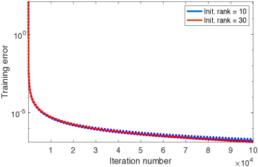
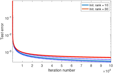
Figure 1: With the setup explained in Example 1.1, this figure shows the training error (left) and test error (right) of the gradient descent (3), when initialized near the origin $(\|U_{0}\|_{\mathrm{F}}=10^{-3})$. The solid and dotted lines show the average over three trials $\pm$ half of the standard deviation, respectively. Note that the implicit bias of the gradient descent (3) towards the planted model $X^{\natural}$ is (slightly) stronger (and the test error is marginally smaller) when the initialization is low-rank.

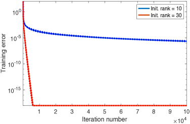
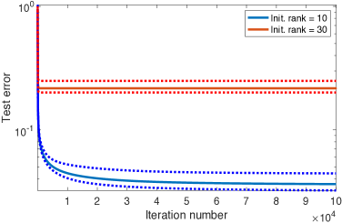
Figure 2: This figure complements Figure 1. With the setup explained in Example 1.1, this figure shows the training error (left) and test error (right) of the gradient descent (3), when initialized further from the origin $(\|U_{0}\|_{\mathrm{F}}=1)$. The solid and dotted lines again show the average over three trials $\pm$ half of the standard deviation, respectively. Note that the implicit bias of the gradient descent (3) towards the planted model $X^{\natural}$ is considerably stronger when the initialization is low-rank. Above, the gradient descent with high-rank initialization terminates after the training error in one of its trials reaches the machine precision.

1.1 Contributions

The numerical Example 1.1 uncovers a new facet about the implicit bias of gradient flow (1), i.e., its sensitivity to the initialization rank. For instance, when initialized high-rank, the flow (1) is in general not implicitly biased towards the planted matrix $X^{\natural}$, see Figure 2. Towards better understanding this new limitation of implicit bias, we partially characterize the implicit bias of the flow (1), when its initialization is low-rank. Informally speaking, our main theoretical finding is that:

When initialized low-rank and with a sufficiently small training (or test) error, the gradient flow (1)

$$\textit{is implicitly biased towards the planted low-rank model }X^{\natural}\textit{, and achieves zero test error.}$$ (4)

After recalling (2), we observe that (4) provides an alternative to the full-rank and nearly-zero initialization scheme of [2, 3, 11]. Note also that both of the assumptions in (4) loosely reflect the real limitations of implicit bias that we numerically identified in Example 1.1:

First, when initialized high-rank, the flow (1) is in general not implicitly biased towards $X^{\natural}$, unless the initialization is near the origin as in (2). Second, if the initial test error is very large, then the initialization is far from the origin (by triangle inequality). In turn, when initialized faraway, we saw in Figure 3 that the flow (1) is in general not implicitly biased towards $X^{\natural}$. As we will see later, our theoretical finding in (4) is also fundamentally different from the local refinement results in signal processing [12, Chapter 5].

To complement the theoretical findings in (4), we also propose a more practical scheme to recover $X^{\natural}$: Indeed, the gist of Example 1.1 and (4) is that both high-rank and high-norm initializations are in general detrimental to implicit bias. This observation later leads us to the following heuristic:

To recover the planted matrix $$X^{\natural}$$, initiate the flow (1) with a random matrix.

If the training error is reducing too rapidly,

then restart the training after decreasing the initialization rank and norm. (5)

We may again think of (5) as an alternative that complements the full-rank and almost-zero initialization scheme that is predominant in the literature of matrix sensing [2, 3, 11], see (2). Let us next present a more detailed, but still simplified, version of our main theoretical result in (4), specialized to the case where $\mathcal{A}$ is a generic linear operator.

Theorem 1.2 (Main result, simplified).

Consider the model $X^{\natural}\in\mathbb{R}^{d\times d}$ and fix an integer $m$. For every $i\leq m$, populate the upper triangular entries of the symmetric matrix $A_{i}\in\mathbb{R}^{d\times d}$ with independent Gaussian random variables that have zero mean and unit variance. In doing so, we obtain a generic sensing operator $\mathcal{A}:\mathbb{R}^{d\times d}\rightarrow\mathbb{R}^{m}$ that maps $X$ to $[\langle A_{1},X\rangle,\cdots,\langle A_{m},X\rangle]^{\top}$. Let $b:=\mathcal{A}(X^{\natural})$ denote the training data. When initialized at $U_{0}\in\mathbb{R}^{d\times d}$, the limit point of the gradient flow (1) exists and achieves zero test error, provided that

1. $m=\Omega(\mathrm{rank}(U_{0})d\log d)$, i.e., $m\gtrsim\mathrm{rank}(U_{0})d\log d$, where $\gtrsim$ suppresses the constants.

2. $\mathrm{rank}(U_{0})\geq\mathrm{rank}(X^{\natural})$.

3. $\|U_{0}\|\leq\sqrt{\|X^{\natural}\|}$, where $\|\cdot\|$ denotes the spectral norm.

4. The initial training (or test) error is not too large. This will be made precise later.

For clarity and insight, it is not uncommon to study the gradient flow (1) as a proxy for its discretization (3), e.g., see [3, 4]. Let us now informally justify the assumptions of Theorem 1.2.

• With overwhelming probability, (i) ensures that the linear operator $\mathcal{A}$ is injective, when restricted to the set of all matrices with rank at most $\mathrm{rank}(U_{0})$ [13, 14]. This restricted injectivity property (RIP) is necessary because, otherwise, the planted model $X^{\natural}$ might not be identifiable from the training data $b=\mathcal{A}(X^{\natural})$. For instance, in the absence of (i), we observe from (ii) that $U_{0}U_{0}^{\top}$ and $X^{\natural}$ might be indistinguishable and both mapped by the operator $\mathcal{A}$ to the same training data $b$ !

  Crucially, in order for (i) to hold in practice, the initialization rank cannot be too large. More specifically, $m$ is in practice often limited by our sampling budget. Therefore, in order to enforce (i), we must in turn select $\mathrm{rank}(U_{0})$ to be relatively small, i.e., $\mathrm{rank}(U_{0})=O(m/(d\log d))$. In this way, Theorem 1.2 reflects the true limitations of implicit bias that we numerically identified in Example 1.1. Indeed, recall that the flow (1) is in general not implicitly biased towards $X^{\natural}$, when its initialization is high-rank, see Figure 2. Lastly, the RIP in (i) is in the same vein as [11, 13].

• (ii) is weaker than $\mathrm{rank}(U_{0})=d$ in [2, 11]. In this sense, Theorem 1.2 is the first result to investigate the implicit bias of the gradient flow (1) in the more general setting where $\mathrm{rank}(U_{0})\geq\mathrm{rank}(X^{\natural})$.

• (iii) reflects the limitations of implicit bias in the following sense: As we observed in the numerical Example 1.1, the flow (1) is in general not implicitly biased towards the planted model $X^{\natural}$, when initialized far from the origin, see Figures 2 and 3. At the same time, recall also from (2) that [2, 3, 11] only study an almost-zero initialization for the flow (1). Compared to these works, Theorem 1.2 is the first result to investigate the implicit bias of (1) beyond the vanishing initialization norm in (2).

• Likewise, (iv) also partially mirrors the limitations of implicit bias in the following sense: It follows from the triangle inequality that an initialization $U_{0}$ with a large test error ($\|U_{0}U_{0}^{\top}-X^{\natural}\|_{\mathrm{F}}\gg\|X^{\natural}\|_{\mathrm{F}}$) is also far from the origin ($\|U_{0}\|_{\mathrm{F}}\gg 0$). In turn, as we saw earlier in Figures 2 and 3, in general the gradient flow (1) is not implicitly biased towards $X^{\natural}$, when initialized faraway from the origin.

  We emphasize that Theorem 1.2 is an example of a “capture theorem” within the literature of nonconvex optimization [15, 16, 17, 18]. As is standard, our capture theorem predicates on an initialization within a specific “capture neighborhood” of the set of matrices with zero training error, i.e., our result predicates on an initialization within a certain neighborhood of the set $\{U:\mathcal{A}(UU^{\top})=b\}$.

  Such capture theorems are fundamentally different from the local refinement results, within the signal processing literature. The latter group of results often rely on local strong convexity in a very small neighborhood of a matrix with zero test error [12, Chapter 5]. In contrast, our capture neighborhood contains all matrices with zero training error (which of course includes all matrices with zero test error). We can visualize this capture neighborhood as a “tube” $\{U:\|\mathcal{A}(UU^{\top}-\underline{U}\,\underline{U}^{\top})\|_{2}\leq\rho\}$ rather than a small Euclidean ball centered at a matrix $\underline{U}$ with zero test error ($\underline{U}\,\underline{U}^{\top}=X^{\natural}$).

To summarize, this work is a small step towards better understanding the limitations of implicit bias in matrix sensing. Here, we identify and partially quantify the sensitivity of implicit bias to the initialization rank. We also propose an adaptive heuristic for matrix sensing which complements the predominant high-rank and near-zero initialization scheme [2, 3, 11]. Beyond matrix sensing, a near-zero initialization often leads to vanishing gradients in deep learning [19]. Alternatives to (2), such as our (5), might in the future provide valuable insights for more difficult learning problems.

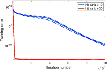
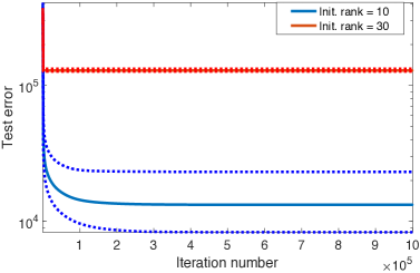
Figure 3: This figure complements Figures 1 and 2. With the setup explained in Example 1.1, this figure shows the training error (left) and test error (right) of the gradient descent (3), when initialized much further from the origin $(\|U_{0}\|_{\mathrm{F}}=10^{3})$. The solid and dotted lines again show the average over three trials $\pm$ half of the standard deviation. Note that the test error is large for both initialization ranks, i.e., the gradient descent (3) is not implicitly biased towards the planted model $X^{\natural}$. Nevertheless, the test error is smaller when the initialization is low-rank.

2 Objective and Assumptions

Here, we set the stage for our detailed main result. For $\xi>0$, consider a model $X^{\natural}\in\mathbb{R}^{d\times d}$ such that

$$0\preceq X^{\natural}\prec\xi^{2}I_{d},$$ (model)

where $I_{d}\in\mathbb{R}^{d\times d}$ is the identity matrix, and $A\preceq B$ means that $B-A$ is a positive semi-definite (PSD) matrix. Likewise, $A\prec B$ means that $B-A$ is a positive definite matrix. As suggested by (model), we limit ourselves to PSD matrices throughout, similar to [2, 11]. Note also that (model) conveniently assumes a priori knowledge of (an estimate of) $\|X^{\natural}\|$, where $\|\cdot\|$ stands for the spectral norm. To gauge the complexity of a model, we will rely on rank and effective rank, defined below.

Definition 2.1 (Effective rank).

The effective rank of a PSD matrix $X$, denoted throughout by $\mathrm{effrank}(X)$, is the smallest integer $r$ such that there exists a PSD matrix $X_{r}$, of rank at most $r$, that is infinitesimally close to $X$. In particular, $\|X-X_{r}\|_{\mathrm{F}}\leq\epsilon\|X\|_{\mathrm{F}}$ for an infinitesimal $\epsilon$. The effective rank and (standard) rank are related as $\mathrm{effrank}\leq\mathrm{rank}$.

The subtle distinction between $\mathrm{rank}$ and $\mathrm{effrank}$ is only for technical correctness, which the reader may ignore in a first reading. The closely related concepts of numerical or approximate rank and border rank are discussed in  [20, Page 275] and [21, Section 3.3]. For symmetric matrices $\{A_{i}\}_{i=1}^{m}\subset\mathbb{R}^{d\times d}$, consider the linear operator $\mathcal{A}:\mathbb{R}^{d\times d}\rightarrow\mathbb{R}^{m}$ and the vector $b\in\mathbb{R}^{m}$, defined as

$$\mathcal{A}(X):=[\langle A_{1},X\rangle,\cdots,\langle A_{m},X\rangle]^{\top},\qquad b:=\mathcal{A}(X^{\natural}).$$ (sense)

In the context of matrix sensing [1], we may think of $\mathcal{A}$ and $b$ as the sensing operator and the training data, respectively. Given the linear operator $\mathcal{A}$ and the training data $b$ in (sense), the objective of this work is to recover $X^{\natural}$ in (model), up to an infinitesimal error. Towards that objective, for an integer $p\geq\mathrm{rank}(X^{\natural})$, it is convenient to define the maps $g:\mathbb{R}^{d\times p}\rightarrow\mathbb{R}^{m}$ and $G:\mathbb{R}^{d\times p}\rightarrow\mathbb{R}$ as

$$g(U):=\frac{1}{2}(\mathcal{A}(UU^{\top})-b),\qquad G(U):=\frac{1}{8}\|\mathcal{A}(UU^{\top})-b\|_{2}^{2}.$$ (training error)

In words, $G$ is the (scaled) training error associated with the model $UU^{\top}$, i.e., $G$ gauges the discrepancy between the sensed vector $\mathcal{A}(UU^{\top})$ and the training data $b$. In particular, $G(U)=0$ if and only if the training error is zero, i.e., $G(U)=0$ iff $\mathcal{A}(UU^{\top})=b$. Note also that $G$ above might be a nonconvex function of $U$. Next, consider the set

$${\mathcal{M}_{b}} :=\{U:\mathcal{A}(UU^{\top})=b,\,\|U\|\leq\xi\}=\{U:G(U)=0,\,\|U\|\leq\xi\}\subset\mathbb{R}^{d\times p},$$ (manifold)

and note that every matrix $U\in\mathcal{M}_{b}$ corresponds to a model $UU^{\top}\in\mathbb{R}^{d\times d}$ with zero training error ($\mathcal{A}(UU^{\top})=b$). Put differently, $\mathcal{M}_{b}$ is the set of all matrices, like $U$, that have zero training error ($G(U)=0$) and satisfy $\|U\|\leq\xi$, as visualized in Figure 4. To recover $X^{\natural}$ in (model) from $\mathcal{A}$ and $b$ in (sense), we will use gradient flow to minimize the (training error). More formally, consider

$$\min_{U\in\mathbb{R}^{d\times p}}\,G(U)={\frac{1}{8}\|\mathcal{A}(UU^{\top})-b\|_{2}^{2}},$$ (ERM)

where ERM stands for empirical risk minimization [22], and above we used the definition of $G$ in (training error). To recover $X^{\natural}$, we apply the gradient flow to (ERM) and obtain

$$\dot{U}(t) =-\nabla G(U(t))=-\frac{1}{2}\mathcal{A}^{*}\left(\mathcal{A}(U(t)U(t)^{\top})-b\right)U(t),\qquad U(0)=U_{0}\in\mathbb{R}^{d\times p}.$$ (flow)

where $\mathcal{A}^{*}:\mathbb{R}^{m}\rightarrow\mathbb{R}^{d\times d}$ denotes the adjoint of the operator $\mathcal{A}$ in (sense).

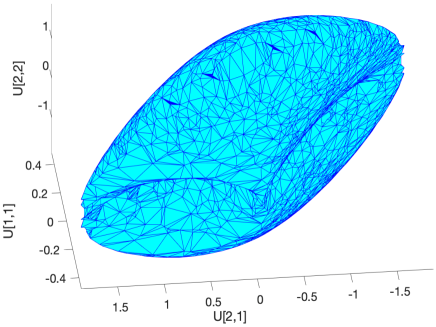
Figure 4: This figure visualizes parts of the set $\mathcal{M}_{b}$ for a toy example. Defined in (manifold), recall that $\mathcal{M}_{b}$ is the set of all matrices with zero training error and bounded norm. Above, $d=p=m=2$ and $X^{\natural}\in\mathbb{R}^{d\times d}$ in (model) is a random matrix of rank $r=1$. The linear operator $\mathcal{A}:\mathbb{R}^{d\times d}\rightarrow\mathbb{R}^{m}$ takes $UU^{\top}\in\mathbb{R}^{d\times d}$ to $\mathcal{A}(UU^{\top})=[\|U[1,:]\|_{2}^{2}\,\,\langle A,UU^{\top}\rangle]^{\top}\in\mathbb{R}^{m}$ for a random matrix $A\in\mathbb{R}^{2\times 2}$. Here, $U[1,:]$ is the first row of $U$ in MATLAB notation. Even though $\mathcal{M}_{b}$ is a subset of $\mathbb{R}^{d\times p}$, the particular structure of $\mathcal{A}$ in this toy example allows us to visualize this set. More specifically, for every $U\in\mathcal{M}_{b}$, the constraints $\mathcal{A}(UU^{\top})=b$ in (manifold) determine the $\ell_{2}$-norm of the first row of $U$. Consequently, above we plot only three entries of the matrix $U$, namely, $U[1,1]$, $U[2,1]$ and $U[2,2]$ in MATLAB notation. The three-dimensional mesh has been created with help from [23].

A crucial observation is the following: Under our key Assumption 3.1 below, the set $\mathcal{M}_{b}$ in (manifold) may contain infinitely many distinct matrices with zero training error but nonzero test error, see Example 1.1. That is, there might exist infinitely many matrices like $U\in\mathbb{R}^{d\times p}$ that satisfy $\mathcal{A}(UU^{\top})=b$, but $UU^{\top}$ is far from the planted model $X^{\natural}$. Put differently, under Assumption 3.1, problem (ERM) might have infinitely many global minimizers, like $U$, that reach the optimal value zero of problem (ERM), but $UU^{\top}$ is far from the planted model $X^{\natural}$. Indeed, note that problem (ERM) lacks any explicit bias towards $X^{\natural}$ (such as regularization with the trace norm [1]). Nevertheless, does the (flow) recover $X^{\natural}$? We answer this question in Section 3 and then compare our main result with the existing literature in Section 4.

3 Main Result

Our main result below posits that, when initialized properly, the (flow) converges to a limit point with zero test error, thus successfully recovering the planted model $X^{\natural}$. We first collect our assumptions.

Assumption 3.1.

Consider the framework specified by (model) and (sense). For an integer $p$, consider also the (flow), initialized at $U_{0}\in\mathbb{R}^{d\times p}$.

1. (Recoverable). Assume that $m/d\leq\mathrm{rank}(X^{\natural})\leq p$.

2. (Manifold). Assume that $\mathrm{rank}(\Delta\rightarrow\mathcal{A}(\Delta U^{\top}))=m$, for every $U$ that belongs to an open neighborhood of the set $\mathcal{M}_{b}$ in (manifold). Equivalently, assume that the matrices $\{A_{i}U\}_{i=1}^{m}$ span an $m$-dimensional subspace of $\mathbb{R}^{d\times p}$, for every $U$ in an open neighborhood of $\mathcal{M}_{b}$.

3. (Restricted injectivity). Assume that the linear operator $\mathcal{A}$ in (sense) satisfies the $(2\mathrm{rank}(U_{0}))$-restricted injectivity property, abbreviated as $(2\mathrm{rank}(U_{0}))$-RIP. More specifically, we assume that $\mathcal{A}(X)=0\Longrightarrow X=0$, for every PSD matrix $X$ with $\mathrm{rank}(X)\leq 2\mathrm{rank}(U_{0})$. We let $\alpha$ denote the corresponding isometry constant, i.e., $\alpha:=\min\{\|\mathcal{A}(X)\|_{\mathrm{F}}:\|X\|_{\mathrm{F}}=1,\,\mathrm{rank}(X)\leq 2\mathrm{rank}(U_{0})\}$.

4. Assume that $\mathrm{rank}(U_{0})\geq\mathrm{effrank}(X^{\natural})$,

5. Recall $\xi$ from (model). Assume that $U_{0}$ satisfies $\|U_{0}\|\leq\xi$ and any of the inequalities

   $$\|\mathcal{A}(U_{0}U_{0}^{\top})-b\|_{2}<\frac{\sigma_{m}(\mathcal{M}_{b})\sigma_{\min}(\mathcal{M}_{b})\alpha}{4\|\mathcal{A}\|},\qquad\text{(initial training error)}$$ (6a)

   $$\|U_{0}U_{0}^{\top}-X^{\natural}\|_{\mathrm{F}}<\frac{\sigma_{m}(\mathcal{M}_{b})\sigma_{\min}(\mathcal{M}_{b})\alpha}{4\|\mathcal{A}\|^{2}},\qquad\text{(initial test error)}$$ (6b)

   $$\operatorname{dist}(U_{0},\mathcal{M}_{b})<\frac{\sigma_{m}(\mathcal{M}_{b})}{4\|\mathcal{A}\|}\min\left(1,\frac{\sigma_{\min}(\mathcal{M}_{b})\alpha}{4\xi\|\mathcal{A}\|}\right).\qquad\text{(initial distance to $\mathcal{M}_{b}$)}$$ (6c)

   Above, $\sigma_{m}(\mathcal{M}_{b}):=\min\{\sigma_{m}(\Delta\rightarrow\mathcal{A}(\Delta U^{\top})):U\in\mathcal{M}_{b}\}$, where $\sigma_{m}(\cdot)$ returns the $m$th largest singular value of an operator. Also, $\sigma_{\min}(\mathcal{M}_{b}):=\min\{\sigma_{\min}(U):U\in\mathcal{M}_{b}\}$, where $\sigma_{\min}(\cdot)$ returns the smallest nonzero singular value of an operator. Lastly, $\alpha$ is the isometry constant and the operator norm of the linear operator $\mathcal{A}$ in (sense), respectively.

Theorem 3.2 (Implicit bias, main result).

Consider the framework specified by (model) and (sense). Suppose that Assumption 3.1 is fulfilled. Then the (flow) converges to a limit point $\underline{U}\in\mathbb{R}^{d\times p}$ such that $\underline{U}\,\underline{U}^{\top}$ is infinitesimally close to $X^{\natural}$ in (model).

We refer to Section 1.1 for insights, and to Section 4 for comparison with the literature. As discussed in Remark 3.6, the right-hand sides of (6) are often difficult to estimate in practice. Indeed, Theorem 3.2 primarily provides theoretical insights and will later be complemented with a practical algorithm.

Remark 3.3 (Proof outline).

At a high level, we follow a two-pronged approach:  We establish that the (flow) solves problem (ERM) in the limit of $t\rightarrow\infty$. That is, we show that the limit point of the (flow) exists and has zero training error.   We also show that rank does not increase along the (flow), which allows us to prove that the test error of the (flow) also vanishes in limit and that we recover the planted model $X^{\natural}$, as desired. The details are deferred to the appendix.

Remark 3.4 (Recoverable).

The inequality $\mathrm{rank}(X^{\natural})\leq p$ in Assumption 3.1(i) is a trivial assumption which ensures that the set $\mathcal{M}_{b}$ in (manifold) is not empty. In particular, Assumption 3.1(i) ensures that there exists a matrix $U\in\mathbb{R}^{d\times p}$ such that $\mathcal{A}(UU^{\top})=b$. That is, under Assumption 3.1(i), the optimal value of (ERM) is zero and there exists a matrix $U\in\mathbb{R}^{d\times p}$ with zero (training error). Note that [2, 3, 11] set $p=d$ and this condition is thus met immediately.

On the other hand, the inequality $m/d\leq\mathrm{rank}(X^{\natural})$ in Assumption 3.1(i) is a mild technical assumption for the proofs. If not met at first, this inequality can be easily enforced by infinitesimally perturbing $X^{\natural}$, as long as $m\leq pd$. Note that this perturbation does not change $\mathrm{effrank}(X^{\natural})$, see Definition 2.1. Only $\mathrm{effrank}(X^{\natural})$ is of statistical significance, and not $\mathrm{rank}(X^{\natural})$. Lastly, the simpler under-parametrized regime of $m>pd$ is not of interest here and we refer the reader to the survey [12].

Remark 3.5 (Manifold).

Assumption 3.1(ii) corresponds to the well-known linear independence constraint qualifications (LICQs) for the feasibility problem

$$\textup{find }U\textup{ such that }\mathcal{A}(UU^{\top})=b,$$ (7)

which attempts to find a matrix $U$ with zero (training error), i.e., a matrix $U$ that satisfies $G(U)=0$. Assumption 3.1(ii) corresponds to the weakest sufficient conditions under which the KKT conditions are necessary for feasibility in (7), see [24, 25]. Without Assumption 3.1(ii), the (training error) is not necessarily dominated by its gradient $(\nabla G(U)=0\not\Rightarrow G(U)=0)$, in which case we cannot in general hope to solve (7) in polynomial time with a first-order optimization algorithm.

That is, without Assumption 3.1(ii), we cannot in general hope to efficiently find any matrix that achieves zero training error! Such peculiarities are not uncommon in nonconvex optimization [26]. From this perspective, Assumption 3.1(ii) is minimal in order to successfully recover the planted model $X^{\natural}$.

See also [15, 16, 27] for precedents of Assumption 3.1(ii). Beyond LICQs, the supplementary relates Assumption 3.1(ii) to other notions in optimization theory, e.g., the Polyak-Łojasiewicz condition [28, 29]. As a side note, if Assumption 3.1(ii) is fulfilled, then $\mathrm{int}(\mathcal{M}_{b})$ is a closed embedded submanifold of $\mathbb{R}^{d\times p}$ with co-dimension $m$ [30, Corollary 5.24]. Here, $\mathrm{int}(\cdot)$ stands for the relative interior of a set.

The appendix also establishes that Assumption 3.1(ii) holds almost surely for the generic linear operator $\mathcal{A}$ that was described in Theorem 1.2, provided that $m=\Omega(\mathrm{rank}(U_{0})d\log d)$, i.e., provided that the problem is sufficiently over-parametrized.

Beyond the common choice for the operator $\mathcal{A}$ in Theorem 1.2, verifying Assumption 3.1(ii) is often difficult in practice, even though this assumption has several precedents within the nonconvex optimization literature, e.g., [15, 16, 27]. In this sense, Theorem 3.2 should be regarded primarily as a theoretical result that sheds light, for the first time, on the role of initialization rank in the implicit bias of gradient flow in matrix sensing.

Remark 3.6 (Initialization rank).

The RIP in Assumption 3.1(iii) is common in matrix sensing and ensures that the operator $\mathcal{A}$ acts as an injective map, when its domain is restricted to sufficiently low-rank matrices [1]. For example, the generic linear operator $\mathcal{A}:\mathbb{R}^{d\times d}\rightarrow\mathbb{R}^{m}$ in Theorem 1.2 satisfies the $r$-RIP, provided that $m={\Omega}(rd\log d)$ [13, Theorem 2][14].

Considering our (often) limited sampling budget, we must in practice select a sufficiently low-rank initialization for the (flow) to ensure that Assumption 3.1(iii) is fulfilled. For example, for the generic operator $\mathcal{A}$ in Theorem 1.2, we must initialize the (flow) at $U_{0}$ such that $\mathrm{rank}(U_{0})=O(m/(d\log d))$.

Therefore, Assumption 3.1(ii) correctly reflects the limitations of implicit bias of the (flow). Indeed, we observed numerically in Example 1.1 that, with a high-rank initialization, the (flow) is in general not implicitly biased towards $X^{\natural}$. The exception is when the initialization is also nearly zero as in (2).

Remark 3.7 (Initialization norm).

An initialization $U_{0}$ that satisfies Assumptions 3.1(iv)-(v) exists under mild conditions, e.g., by appealing to the Pataki’s lemma [31, 32]. Note that Theorem 3.2 is an example of a “capture theorem” in nonconvex optimization [15, 16, 17, 18], i.e., Theorem 3.2 predicates on an initialization within a specific “capture neighborhood” of the set $\mathcal{M}_{b}$ in (manifold). Equivalently, Theorem 3.2 predicates on an initialization within a sufficiently small neighborhood of the set of all matrices with zero training error, see (6c). As stipulated in (6a)-(6b), this neighborhood also coincides with the set of all matrices with a sufficiently small training (or test) error.

Phrased differently, Theorem 3.2 applies only when the (flow) is initialized sufficiently close to the set $\mathcal{M}_{b}$ in (manifold), see (6c). Equivalently, in light of (6a) and (6b), Theorem 3.2 applies only when the training or test error is sufficiently small at the initialization.

Assumption 3.1(v) partially reflects the limitations of implicit bias, and loosely agrees with our numerical observation in Example 1.1 that there is no implicit bias when the (flow) is initialized far from the origin, see Figure 3. To illustrate this connection, let us focus only on (6a). Note that

$$\|U_{0}\|^{2}=\|U_{0}U_{0}^{\top}\| \geq\|U_{0}U_{0}^{\top}-X^{\natural}\|-\|X^{\natural}\|\geq\|U_{0}U_{0}^{\top}-X^{\natural}\|-\xi$$

$$\geq{\left|\kern-1.07639pt\left|\kern-1.07639pt\left|\mathcal{A}\right|\kern-1.07639pt\right|\kern-1.07639pt\right|}^{-1}\cdot\|\mathcal{A}(U_{0}U_{0}^{\top}-X^{\natural})\|_{2}-\xi={\left|\kern-1.07639pt\left|\kern-1.07639pt\left|\mathcal{A}\right|\kern-1.07639pt\right|\kern-1.07639pt\right|}^{-1}\cdot\|\mathcal{A}(U_{0}U_{0}^{\top})-b\|_{2}-\xi,$$ (8)

where ${\left|\kern-1.07639pt\left|\kern-1.07639pt\left|\mathcal{A}\right|\kern-1.07639pt\right|\kern-1.07639pt\right|}$ is the appropriate operator norm of $\mathcal{A}$, and we repeatedly used (model) and (sense) above. In view of (8), if the initial training error is large $(\|\mathcal{A}(U_{0}U_{0}^{\top})-b\|_{2}\gg{\left|\kern-1.07639pt\left|\kern-1.07639pt\left|\mathcal{A}\right|\kern-1.07639pt\right|\kern-1.07639pt\right|}\xi)$, then the initialization norm will be large $(\|U_{0}\|_{\mathrm{F}}\gg 0)$ and the (flow) will in general show no implicit bias towards the planted model $X^{\natural}$, as we saw numerically in Figure 3. We lastly note that Assumption 3.1(v) is difficult to verify in practice and, as discussed in Remark 3.5, Theorem 3.2 should therefore be regarded primarily as a theoretical result that sheds light on the role of initialization rank in implicit bias.

Remark 3.8 (Local refinement).

Capture theorems, such as Theorem 3.2, are fundamentally different from the local refinement results within the signal processing literature. Such local refinement results require us to initialize the (flow) within a very small neighborhood of a matrix with zero test error, in which local strong convexity holds [12, Chapter 5]. In contrast, our capture neighborhood in (6a) contains all matrices with zero training error (which also of course includes all matrices with zero test error). In fact, we observe from (6a) that the capture neighborhood in Theorem 3.2 is a “tube” of the form $\{U:\|\mathcal{A}(UU^{\top}-\underline{U}\,\underline{U}^{\top})\|_{2}\leq\rho\}$ for a certain radius $\rho$, rather than a small Euclidean ball centered at a matrix $\underline{U}$ that has zero test error $(\underline{U}\,\underline{U}^{\top}=X^{\natural})$.

Remark 3.9 (Proof of Theorem 1.2).

To establish Theorem 1.2 as a corollary of Theorem 3.2, it suffices to verify that Assumption 3.1 is fulfilled. Because $p=d$ in Theorem 1.2, Assumption 3.1(i) is met trivially, possibly after infinitesimally perturbing $X^{\natural}$, see Remark 3.4. Assumptions 3.1(ii)-(iii) hold with overwhelming probability in view of Theorem 1.2(i) and Remarks 3.5 and 3.6. Assumption 3.1(iv) holds by Theorem 1.2(ii) and $\mathrm{effrank}\leq\mathrm{rank}$. Lastly, Assumption 3.1(v) holds by Theorem 1.2(iii)-(iv).

4 Related Work

Under various assumptions on the operator $\mathcal{A}$ in (sense), [2, 3, 11] have studied the implicit bias of the (flow) in matrix sensing, see also [33, 34, 35, 36, 13]. In particular, for a specially designed operator $\mathcal{A}$, for which $\mathcal{M}_{b}$ in (manifold) aligns with the level sets of the convex matrix sensing problem, [13] proved that the planted model $X^{\natural}$ is the unique PSD matrix that satisfies $\mathcal{A}(X^{\natural})=b$. For our purposes, the most relevant past result is Theorem 1.1 in [11], adapted below to our setup.

Theorem 4.1 (State of the art, simplified).

Consider the framework specified by (model) and (sense). Suppose that the operator $\mathcal{A}$ satisfies the $(4\cdot\mathrm{rank}(X^{\natural}))$-RIP. Suppose also that $p=d$, and that the (flow) is initialized at $U_{0}=u_{0}I_{d}\in\mathbb{R}^{d\times d}$ for a sufficiently small $u_{0}>0$, where $I_{d}$ denotes the identity matrix. Then it holds that

$$\|U(t)U(t)^{\top}-X^{\natural}\|_{\mathrm{F}}^{2}\lesssim u_{0}\sqrt{d}/\kappa(X^{\natural})^{2},\qquad\forall t\in[\kappa(X^{\natural})\log(d/u_{0}),1/\sqrt{u_{0}d\cdot\kappa(X^{\natural})}]$$ (9)

where $\kappa(X^{\natural})$ is the condition number of $X^{\natural}$, i.e., the ratio of its largest and smallest nonzero singular values. Above, $\lesssim$ suppresses any unnecessary factors.

Note that Theorem 4.1 is limited to the case $p=d$, and does not guarantee the convergence of the (flow) to the planted model $X^{\natural}$. Intuitively, when initialized near the origin, the (flow) moves rapidly along the “signal” directions and $U(t)U(t)^{\top}$ approaches a small neighborhood of $X^{\natural}$. After this initial phase, the contribution of “noise” directions might potentially accumulate and push $U(t)U(t)^{\top}$ away from the planted model $X^{\natural}$. (We never observed this divergence numerically.)

There are more fundamental differences between our Theorem 3.2 and Theorem 4.1 from [11]. In the latter, the initialization is full-rank and near-zero. In contrast, as discussed in Remarks 3.6 and 3.7, our Theorem 3.2 applies to a low-rank initialization with a sufficiently small training (or test) error. In Remarks 3.6 and 3.7, we also explained that our requirements on the initialization rank and norm (partially) mirror the true limitations of implicit bias that we had earlier identified in Example 1.1.

Theorem 3.2 can also be used to slightly improve upon Theorem 4.1: For a sufficiently small $u_{0}$ and a sufficiently large $t_{0}$, suppose that $\mathrm{rank}(U(t_{0}))\leq 2\mathrm{rank}(X^{\natural})$. Then it is easy to see that Theorem 4.1 can be strengthened to $\lim_{t\rightarrow\infty}\|U(t)U(t)^{\top}-X^{\natural}\|_{\mathrm{F}}=0$, provided that Assumption 3.1(ii) holds.

This work identifies the limitations of the implicit bias of gradient flow in matrix sensing. For limitations of implicit bias in other settings, among others, see [37] for shallow neural networks, [38] for stochastic convex optimization, and [39] for matrix completion, where the RIP never holds.

5 A New Algorithm for Matrix Sensing

We emphasize that Theorem 3.2 primarily provides theoretical insights, shedding light for the first time on the role of the initialization rank in implicit bias. To complement Theorem 3.2, we next propose an adaptive heuristic for matrix sensing that replaces Assumption 3.1(v) with a more practical guideline. This new algorithm complements the full-rank and near-zero initialization scheme that has dominated the existing literature of implicit bias in matrix sensing [2, 3, 11], see (2). Beyond matrix sensing, a near-zero initialization often leads to vanishing gradients in deep learning [19]. In that sense, alternatives to (2), such as the new algorithm below, might in the future provide valuable insights for more difficult learning problems.

The message of Example 1.1 and Theorem 3.2 is that high-rank and high-norm initializations are in general both detrimental to implicit bias. Another remarkable pattern which emerges from an inspection of Figures 1 and 2 is that the test error is always large (no implicit bias), whenever the training error reduces too rapidly. The previous two observations naturally suggest an adaptive heuristic for matrix sensing which restarts the training whenever the convergence is too fast. Figure 5 illustrates a typical outcome, where the new algorithm considerably outperforms the gradient descent (3) with the same initialization. The setup is identical to Example 1.1, but the random data is fresh and $\|U_{0}\|_{\mathrm{F}}=10$, $\eta=5\cdot 10^{-6}$, $W=100$, $\tau=0.998$, $r_{0}=30$, $\Delta_{\mathrm{rank}}=3$, $\text{factor}=1/2$, $r=2$.

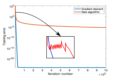
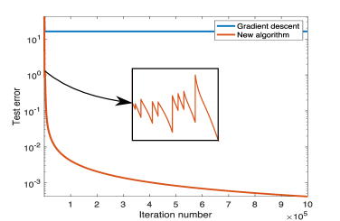
Figure 5: The restarts of the new algorithm are magnified, see Section 5 and the MATLAB code.

Input: The framework specified by (model) and (sense), $\eta>0$, $K,W\in\mathbb{N}$, $W\leq K$, $\tau\geq 0$, $r_{0}\leq d$, $\rho_{0}\geq 0$, $\Delta_{\text{rank}}\in\mathbb{N}$, $\text{factor}\in(0,1)$, $r\geq\mathrm{rank}(X^{\natural})$.

Set $U_{0}\in\mathbb{R}^{d\times p}$ to be a rank-$r_{0}$ matrix inside $\operatorname{ball}(\rho_{0}):=\{U:\|U\|_{\mathrm{F}}\leq\rho_{0}\}$.

For $k=0,1,\cdots,K$, repeat

1. $U_{k+1}=U_{k}-\eta\nabla\|\mathcal{A}(U_{k}U_{k}^{\top})-b\|_{2}^{2}$, $\triangleright$ Gradient descent update

2. If $\mod(k,W)=1$, then $\triangleright$ Every $W$ iterations,

   1. $\text{ratio}\leftarrow\underset{k-W+1\leq k^{\prime}\leq k}{\max}\frac{\|\mathcal{A}(U_{k^{\prime}}U_{k^{\prime}}^{\top})-b\|_{2}^{2}}{\|\mathcal{A}(U_{k^{\prime}-1}U_{k^{\prime}-1}^{\top})-b\|_{2}^{2}}$

   2. If $\text{ratio}<\tau$ $\triangleright$ if convergence was linear in the last window, then

      • $\rho_{0}\leftarrow\text{factor}\cdot\rho_{0}$ and $r_{0}\leftarrow\max(r_{0}-\Delta_{\mathrm{rank}},r)$ $\triangleright$ reduce the initialization norm and rank,

      • Set $U_{k+1}\in\mathbb{R}^{d\times p}$ to be a rank-$r_{0}$ matrix inside $\operatorname{ball}(\rho_{0})$. $\triangleright$ and restart the training.

Algorithm 1 A new algorithm for matrix sensing

Appendix A Geometry of the Set $\mathcal{M}_{b}$

This section studies with more depth the geometry of the set $\mathcal{M}_{b}$ and its neighborhood in $\mathbb{R}^{d\times p}$. Let us recall that $\mathcal{M}_{b}$ is the set of all matrices with zero training error and bounded norm, introduced in (manifold) and briefly discussed in Section 2. Recalling the definition of $g$ in (training error), note also that the (total) derivative of $g(U)$ at $U$ is the linear operator $\mathrm{D}g(U):\mathbb{R}^{d\times p}\rightarrow\mathbb{R}^{m}$, defined as

$$\mathrm{D}g(U)[\Delta]:=\mathcal{A}(\Delta U^{\top}),$$ (10)

and its adjoint operator is specified as

$$(\mathrm{D}g(U))^{*}[\delta]:=\mathcal{A}^{*}(\delta)\cdot U=\sum_{i=1}^{m}\delta_{i}A_{i}U,$$ (11)

where $\mathcal{A}^{*}$ is the adjoint of the linear operator $\mathcal{A}$ in (sense) and $\delta_{i}$ is the $i^{\text{th}}$ entry of the vector $\delta\in\mathbb{R}^{m}$. Under Assumption 3.1(ii), $\mathrm{int}(\mathcal{M}_{b})$ is a closed embedded submanifold of $\mathbb{R}^{d\times p}$ of co-dimension $m$, where $\mathrm{int}(\cdot)$ stands for the relative interior. Beyond LICQs in Remark 3.5, Assumption 3.1(ii) is also related to the Polyak-Łojasiewicz (PL) condition [28, 29]. If the compact set $\mathcal{M}_{b}$ in (manifold) satisfies Assumption 3.1(ii), there exists $\mu>0$ such that $G$ in (training error) satisfies

$$\frac{1}{2}\|\nabla G(U)\|_{\mathrm{F}}^{2} =\frac{1}{2}\left\|(\mathrm{D}g(U))^{*}[g(U)]\right\|_{\mathrm{F}}^{2}\qquad\text{(chain rule)}$$

$$\geq\frac{\mu}{2}\|g(U)\|_{2}^{2}=\mu\cdot G(U),$$ (12)

for every $U$ in an open neighborhood of $\mathcal{M}_{b}$. In view of (12), Assumption 3.1(ii) implies the PL condition for the function $G$, when restricted to the a neighborhood of $\mathcal{M}_{b}$, see [28, Equation (3)]. In passing, we also remark that Assumption 3.1 also relates to the Mangasarian-Fromovitz and Kurdyka-Łojasiewicz conditions [40, 41, 16]. Next, consider the generic operator $\mathcal{A}$ described in Theorem 1.2. We assume without loss of generality that $m\leq d^{2}$ because the problem is otherwise trivial. Consequently, for fixed $U\in\mathbb{R}^{d\times d}$, $\{A_{i}U\}_{i=1}^{m}\subset\mathbb{R}^{d\times d}$ are almost surely linearly independent, thanks to the random design of $\mathcal{A}$. Since $\mathcal{M}_{b}$ in (manifold) is a compact set, it also follows that Assumption 3.1(ii) is fulfilled almost surely.

Let us next study the neighborhood of the set $\mathcal{M}_{b}$ in (manifold), beginning below with a more quantitative approach to Assumption 3.1(ii). More specifically, below we define a well-behaved neighborhood of the set $\mathcal{M}_{b}$ in (manifold), the existence of which will shortly be guaranteed under Assumption 3.1(ii). We add that this specific neighborhood of $\mathcal{M}_{b}$, defined below, is of key importance for us. Indeed, as we will see later in this section, any limit point of the (flow), within this well-behaved neighborhood, achieves zero training error.

Definition A.1 (Geometric regularity).

Suppose that Assumption 3.1(ii) holds and fix $\rho\in[0,\infty)$. Recall the map $g$ in (training error). We say that the set $\mathcal{M}_{b}$ in (manifold) satisfies the $(\rho,m)$-geometric regularity or $(\rho,m)$-GR if

$$\min\left\{\sigma_{m}(\mathrm{D}g(U)):\operatorname{dist}(U,{\mathcal{M}_{b}})\leq\rho\right\}>0,$$ (13)

where $\sigma_{i}(\cdot)$ returns the $i^{\text{th}}$ largest singular value of a linear operator, and

$$\operatorname{dist}(U,{\mathcal{M}_{b}}):=\min_{U^{\prime}\in{\mathcal{M}_{b}}}\|U-U^{\prime}\|_{\mathrm{F}}$$ (14)

is the distance from the matrix $U\in\mathbb{R}^{d\times p}$ to the compact set ${\mathcal{M}_{b}}$.

Before we proceed, for completeness, a short remark follows next to justify the choice of metric in Definition A.1.

Remark A.2 (Invariance of the metric).

The metric in  (14) is invariant under rotation from right. That is, for any $U\in\mathbb{R}^{d\times p}$ and $R\in\mathcal{O}_{p}$, it holds that

$$\operatorname{dist}(UR,\mathcal{M}_{b}) =\min_{U^{\prime}\in\mathcal{M}_{b}}\|UR-U^{\prime}\|_{\mathrm{F}}$$

$$=\min_{U^{\prime}\in\mathcal{M}_{b}}\|UR-U^{\prime}R\|_{\mathrm{F}}$$

$$=\min_{U^{\prime}\in\mathcal{M}_{b}}\|U-U^{\prime}\|_{\mathrm{F}}$$

$$=\operatorname{dist}(U,\mathcal{M}_{b}),$$ (15)

where the second line above holds because $U^{\prime}\in\mathcal{M}_{b}$ implies that $U^{\prime}R\in\mathcal{M}_{b}$, see (manifold). The third line holds by the rotational invariance of the Frobenius norm. Here, $\mathcal{O}_{p}=\{R:R^{\top}R=I_{p}\}\subset\mathbb{R}^{p\times p}$ denotes the orthogonal group and $I_{p}\in\mathbb{R}^{p\times p}$ is the identity matrix.

Using a standard perturbation argument, the next result establishes that the set $\mathcal{M}_{b}$ satisfies the geometric regularity, provided that Assumption 3.1(ii) is fulfilled. That is, simply put, Definition A.1 is not vacuous.

Proposition A.3 (Geometric regularity).

If Assumption 3.1(ii) is met, then the set $\mathcal{M}_{b}$ in (manifold) satisfies the $(\rho_{0},m)$-GR with

$$\rho_{0}:=\frac{\sigma_{m}({\mathcal{M}_{b}})}{2\|\mathcal{A}\|},$$ (16)

where $\sigma_{m}({\mathcal{M}_{b}}):=\min\{\sigma_{m}(\mathrm{D}g(U)):U\in{{\mathcal{M}_{b}}}\}>0$ and $\|\mathcal{A}\|$ is the operator norm of $\mathcal{A}$ in (sense). Here, $\sigma_{m}(\mathrm{D}g(U))$ returns the $m^{\text{th}}$ largest singular value of the operator $\mathrm{D}g(U)$.

Let us record below a consequence of (12) and Proposition A.3, which will be later central to the proof of the main result of this paper. In words, the lemma below posits that the (nonconvex) problem (ERM) does not have any spurious first-order stationary points within a neighborhood of the set $\mathcal{M}_{b}$ in (manifold). In particular, the lemma below implies that any limit point of the (flow) within this neighborhood has zero training error.

Lemma A.4 (No spurious FOSP).

Suppose that Assumption 3.1(ii) holds. Then any first-order stationary point (FOSP) of $G$ inside the set $\{U:\operatorname{dist}(U,\mathcal{M}_{b})\leq\rho_{0}\}$ is also a global minimizer of the problem (ERM) (zero training error). That is, if $\underline{U}\in\mathbb{R}^{d\times p}$ satisfies $\nabla G(\underline{U})=0$ and $\operatorname{dist}(\underline{U},\mathcal{M}_{b})\leq\rho_{0}$, then $\mathcal{A}(\underline{U}\,\underline{U}^{\top})=b$. See (sense), (training error) and (16) to review the notation used in this lemma.

Appendix B Proof of Proposition A.3

For $U\in\mathbb{R}^{d\times p}$, let $U_{\mathcal{M}_{b}}\in{\mathcal{M}_{b}}$ be the projection of $U$ onto ${\mathcal{M}_{b}}$, i.e.,

$$\text{dist}(U,{\mathcal{M}_{b}})=\|U-U_{\mathcal{M}_{b}}\|_{\mathrm{F}}\leq\|U-U^{\prime}\|_{\mathrm{F}},\qquad\forall U^{\prime}\in{\mathcal{M}_{b}}.$$ (17)

Above, note that $U_{\mathcal{M}_{b}}$ exists by the compactness of ${\mathcal{M}_{b}}$ in (manifold), but might not be unique. Using the Weyl’s inequality, note also that

$$\sigma_{m}(\mathrm{D}g(U)) \geq\sigma_{m}(\mathrm{D}g(U_{\mathcal{M}_{b}}))-\|\mathrm{D}g(U)-\mathrm{D}g(U_{\mathcal{M}_{b}})\|.$$ (18)

To compute the operator norm of $\mathrm{D}g(U)-\mathrm{D}g(U_{\mathcal{M}_{b}})$ on the far-right above, we note that

$$\|(\mathrm{D}g(U)-\mathrm{D}g(U_{\mathcal{M}_{b}}))[\Delta]\|_{2} =\|\mathcal{A}(\Delta U^{\top})-\mathcal{A}(\Delta U_{\mathcal{M}_{b}}^{\top})\|_{2}\qquad\text{(see \eqref{eq:defnC})}$$

$$=\|\mathcal{A}(\Delta(U-U_{\mathcal{M}_{b}})^{\top})\|_{2}\qquad(\mathcal{A}\text{ is linear})$$

$$\leq\|\mathcal{A}\|\cdot\|\Delta(U-U_{\mathcal{M}_{b}})^{\top}\|_{\mathrm{F}}$$

$$\leq\|\mathcal{A}\|\cdot\|\Delta\|_{\mathrm{F}}\|U-U_{\mathcal{M}_{b}}\|$$

$$\leq\|\mathcal{A}\|\cdot\|\Delta\|_{\mathrm{F}}\|U-U_{\mathcal{M}_{b}}\|_{\mathrm{F}}$$

$$=\|\mathcal{A}\|\cdot\|\Delta\|_{\mathrm{F}}\operatorname{dist}(U,\mathcal{M}_{b}),\qquad\text{(see \eqref{eq:decomposition1})}$$ (19)

for an arbitrary $\Delta\in\mathbb{R}^{d\times p}$. It follows from (19) that

$$\|\mathrm{D}g(U)-\mathrm{D}g(U_{\mathcal{M}_{b}})\|\leq\|\mathcal{A}\|\operatorname{dist}(U,\mathcal{M}_{b}).$$ (20)

Using (20), we can simplify (18) as

$$\sigma_{m}(\mathrm{D}g(U)) \geq\sigma_{m}(\mathrm{D}g(U_{\mathcal{M}_{b}}))-\|\mathcal{A}\|\operatorname{dist}(U,\mathcal{M}_{b})\qquad\text{(see (\ref{eq:bndOnMaxDiff}))}$$

$$\geq\sigma_{m}({{\mathcal{M}_{b}}})-\|\mathcal{A}\|\operatorname{dist}(U,\mathcal{M}_{b}).\qquad\text{(see (\ref{eq:sMinDefn}))}$$ (21)

It immediately follows from (21) that

$$\min\left\{\sigma_{m}(\mathrm{D}g(U)):\operatorname{dist}(U,\mathcal{M}_{b})\leq\rho_{0}:=\frac{\sigma_{m}({{\mathcal{M}_{b}}})}{2\|\mathcal{A}\|}\right\}\geq\frac{\sigma_{m}({{\mathcal{M}_{b}}})}{2}>0,$$ (22)

which completes the proof of Proposition A.3.

Appendix C Proof of Theorem 3.2

Here, we will use Lemma A.4 to prove that the (flow), if initialized properly, converges to a limit point with zero test error. The first lemma in this section states that rank does not increase along the (flow).

Lemma C.1 (Rank of gradient flow).

For an initialization $U_{0}\in\mathbb{R}^{d\times p}$, the (flow) satisfies

$$\mathrm{rank}(U(t))\leq\mathrm{rank}(U_{0}),\qquad t\geq 0.$$ (23)

Proof sketch of Lemma C.1. The claim in Lemma C.1 follows from writing the analytic singular value decomposition (SVD) of $U(t)U(t)^{\top}$, then taking its derivative with respect to time $t$, and finally observing that any zero singular value of $U(t)U(t)^{\top}$ remains zero throughout time. The detailed proof is deferred to the appendix. $\blacksquare$

The next component of our argument posits that the (flow) is bounded. More specifically, when initialized near the set $\mathcal{M}_{b}$ in (manifold), the (flow) always remains near $\mathcal{M}_{b}$, as detailed next.

Lemma C.2 (Flow remains nearby).

Consider an initialization $U_{0}\in\mathbb{R}^{d\times p}$ such that $\|U_{0}\|\leq\xi$ in (model), that $\mathrm{rank}(U_{0})\geq\mathrm{effrank}(X^{\natural})$ and lastly that $\operatorname{dist}(U_{0},\mathcal{M}_{b})$ is not too large, as specified precisely in (50). Suppose that Assumption 3.1(ii) holds. Suppose also that Assumption 3.1(iii) holds with $r\geq{2\cdot\mathrm{rank}(U_{0})}$. Then the (flow) satisfies

$$\operatorname{dist}(U(t),\mathcal{M}_{b})<\rho_{0},\qquad t\geq 0,$$ (24)

where $\rho_{0}$ was defined in (16).

Proof sketch of Lemma C.2. The boundedness of the (flow), claimed in Lemma C.2, follows from two observations:  $G(U(t))=\frac{1}{8}\|\mathcal{A}(U(t)U(t)^{\top})-b\|_{2}^{2}$ in (training error) is evidently bounded because the (flow) moves along the descent direction $-\nabla G(U(t))$.  Under Assumption (iii), the restricted injectivity of the operator $\mathcal{A}$ allows us to translate the boundedness of $G(U(t))$ into the boundedness of $U(t)$ in (flow). A crucial ingredient of the proof is that Lemma C.1 is in force and, consequently, the rank does not increase along the (flow), which in turn allows us to successfully invoke the restricted injectivity of $\mathcal{A}$. $\blacksquare$

In words, Lemma C.2 establishes that the (flow) never escapes the $\rho_{0}$-neighborhood of the set $\mathcal{M}_{b}$ in (manifold). Lemma C.2 will shortly enable us to prove the convergence of the (flow), after recalling the Łojasiewicz’s Theorem below [42, 43].

Theorem C.3 (Łojasiewicz’s Theorem).

If $h:\mathbb{R}^{n}\rightarrow\mathbb{R}$ is an analytic function and the curve $[0,\infty)\rightarrow\mathbb{R}^{n}$, $t\rightarrow z(t)$ is bounded and solves the gradient flow $\dot{z}(t)=-\nabla h(z)$, then this curve converges to an FOSP of $h$.

To apply Theorem C.3, note that $G(U)$ in (training error) is an analytic function of $U$ on $\mathbb{R}^{d\times p}$. Recall also from (manifold) and (24) that the (flow) is bounded. We can now apply Theorem C.3, which asserts that the (flow) converges to an FOSP of $G$, denoted here by $\underline{U}\in\mathbb{R}^{d\times p}$, such that $\operatorname{dist}(\underline{U},\mathcal{M}_{b})\leq\rho_{0}$. In fact, by Lemma A.4, this FOSP $\underline{U}$ has zero training error, that is,

$$\mathcal{A}(\underline{U}\,\underline{U}^{\top})=b.$$ (25)

Moreover, in view of (23) and after using the fact that $\{U:\mathrm{rank}(U)\leq\mathrm{rank}(U_{0})\}$ is a closed set, we find that the limit point $\underline{U}$ of the (flow) also satisfies

$$\mathrm{rank}(\underline{U})\leq\mathrm{rank}(U_{0}).$$ (26)

Informally speaking, we have thus far established that the (flow) has a limit point $\underline{U}$ with zero training error, see (25), and this limit point is low-rank, see (26). We next establish below that $\underline{U}$ also has zero test error.

Let us recall from Lemma C.2 that $\mathrm{rank}(U_{0})\geq\mathrm{effrank}(X^{\natural})$ and that Assumption (iii) holds with $r\geq 2\cdot\mathrm{rank}(U_{0})$. It follows immediately that any matrix $X$ that satisfies $\mathrm{rank}(X)\leq\mathrm{rank}(U_{0})$ and $\mathcal{A}(X)=b=\mathcal{A}(X^{\natural})$ must be infinitesimally close to $X^{\natural}$ in (sense). In view of (25) and (26), we therefore conclude that $\underline{U}\,\underline{U}^{\top}$ is infinitesimally close to $X^{\natural}$. In words, we conclude that the (flow) recovers the planted matrix $X^{\natural}$, up to an infinitesimal error. This completes the proof of Theorem 3.2.

Appendix D Proof of Lemma C.1

For $U\in\mathbb{R}^{d\times p}$, recall the linear operator $\mathrm{D}g(U)$ from (10). The adjoint of this operator is $(\mathrm{D}g(U))^{*}:\mathbb{R}^{m}\rightarrow\mathbb{R}^{d\times p}$, defined as

$$(\mathrm{D}g(U))^{*}[\delta]:=\mathcal{A}^{*}(\delta)\cdot U=\sum_{i=1}^{m}\delta_{i}A_{i}U,$$ (27)

where $\mathcal{A}^{*}$ is the adjoint of the linear operator $\mathcal{A}$ in (sense) and $\delta_{i}$ is the $i^{\text{th}}$ entry of the vector $\delta\in\mathbb{R}^{m}$. For future use, recall also that

$$\nabla G(U_{t}) =(\mathrm{D}g(U_{t}))^{*}[g(U_{t})]=\mathcal{A}^{*}(g(U_{t}))\cdot U_{t},\qquad\text{(see \eqref{eq:fgDefn},\eqref{eq:adjO})}$$ (28)

where we used the shorthand $U_{t}=U(t)$. Let us also define

$$X_{t}:=U_{t}U_{t}^{\top}\in\mathbb{R}^{d\times d},$$ (29)

and note that this new flow in $\mathbb{R}^{d\times d}$ satisfies

$$X_{0} =U_{0}U_{0}^{\top},\qquad\text{(see \eqref{eq:xFlow})}$$

$$\dot{X}_{t} =\dot{U}_{t}U_{t}^{\top}+U_{t}\dot{U}_{t}^{\top}\qquad\text{(see \eqref{eq:xFlow})}$$

$$=-\nabla G(U_{t})\cdot U_{t}^{\top}-U_{t}(\nabla G(U_{t}))^{\top}\qquad\text{(see \eqref{eq:flowG})}$$

$$=-\mathcal{A}^{*}(g(U_{t}))X_{t}-X_{t}\mathcal{A}^{*}(g(U_{t})).\qquad\text{(see (\ref{eq:DerhGammaExplicitRecall}),\eqref{eq:xFlow})}$$ (30)

In the last identity above, we used the fact that $\{A_{i}\}_{i}$ are symmetric matrices in (sense). The next technical result establishes that the flow (30) has an analytic SVD.

Lemma D.1 (Analytic SVD).

The flow (30) has the analytic SVD

$$X_{t}\overset{\text{SVD}}{=}V_{t}S_{t}V_{t}^{\top},\qquad t\geq 0,$$ (31)

where $V_{t}\in\mathbb{R}^{d\times d}$ is an orthonormal basis and the diagonal matrix $S_{t}\in\mathbb{R}^{d\times d}$ contains the singular values of $X_{t}$ in no particular order. Moreover, $V_{t}$ and $S_{t}$ are analytic functions of $t$ on $[0,\infty)$.

Proof. In view of (training error), $G(U)$ is an analytic function of $U$ in $\mathbb{R}^{d\times p}$. It then follows from Theorem 1.1 in [44] that the flow (flow) is an analytic function of $t$ on $[0,\infty)$. Consequently, $X_{t}=U_{t}U_{t}^{\top}$ is an analytic function of $t$ on $[0,\infty)$, see (29). It finally follows from Theorem 1 in [45] that $X_{t}$ thus has an analytic SVD on $[0,\infty)$, as claimed. This completes the proof of Lemma D.1. $\blacksquare$

By taking the derivative with respect to $t$ of both sides of (31), we find that

$$\dot{X}_{t}=\dot{V}_{t}S_{t}V_{t}^{\top}+V_{t}\dot{S}_{t}V_{t}^{\top}+V_{t}S_{t}\dot{V}_{t}^{\top},\qquad t\geq 0.$$ (32)

By multiplying both sides above by $V_{t}^{\top}$ and $V_{t}$ from left and right, we reach

$$V_{t}^{\top}\dot{X}_{t}V_{t} =V_{t}^{\top}\dot{V}_{t}S_{t}+\dot{S}_{t}+S_{t}\dot{V}_{t}^{\top}V_{t},\qquad t\geq 0,$$ (33)

where we used on the right-hand side above the fact that $V_{t}$ is an orthonormal basis, i.e., $V_{t}^{\top}V_{t}=I_{d}$. Taking derivative of both sides of the last identity also yields that

$$\dot{V}_{t}^{\top}V_{t}+V_{t}^{\top}\dot{V}_{t}=0,\qquad t\geq 0,$$ (34)

i.e., $V_{t}^{\top}\dot{V}_{t}$ is a skew-symmetric matrix. In particular, both $\dot{V}_{t}^{\top}V_{t}$ and $V_{t}^{\top}\dot{V}_{t}$ are hollow matrices, i.e., with zero diagonal entries. By taking the diagonal part of both sides of (33), we therefore arrive at

$$\dot{s}_{t,i} =v_{t,i}^{\top}\dot{X}_{t}v_{t,i},\qquad t\geq 0,$$ (35)

where $s_{t,i}$ is the $i^{\text{th}}$ singular value of $X_{t}$ and $v_{t,i}\in\mathbb{R}^{d}$ is the corresponding singular vector. By substituting above the expression for $\dot{X}_{t}$ from (30), we find that

$$\dot{s}_{t,i} =-2s_{t,i}\cdot v_{t,i}^{\top}\mathcal{A}^{*}(g(U_{t}))v_{t,i},\qquad t\geq 0,\qquad\text{(see (\ref{eq:xFlowDer}),(\ref{eq:singEvolvRawe}))}$$ (36)

where above we used the fact that $(s_{t,i},v_{t,i})$ is a pair of singular value and its corresponding singular vector for $X_{t}$. In view of the evolution of singular values given by (36), it is evident that

$$\mathrm{rank}(U_{t})=\mathrm{rank}(X_{t})\leq\mathrm{rank}(X_{0})=\mathrm{rank}(U_{0}),\qquad t\geq 0,\qquad\text{(see \eqref{eq:xFlow})}$$ (37)

which completes the proof of Lemma C.1. The two identities above follow from (29).

Appendix E Proof of Lemma C.2

In view of Definition 2.1, recall $X^{\natural}$ in (model) and fix $X^{\natural}_{l}$ such that

$$\mathrm{rank}(X^{\natural}_{l})=\mathrm{effrank}(X^{\natural}),\qquad\|X^{\natural}-X^{\natural}_{l}\|_{\mathrm{F}}\leq\epsilon\|X^{\natural}\|_{\mathrm{F}},$$ (38)

for an infinitesimal $\epsilon$. Also recall from Assumption 3.1(i) that $\mathrm{rank}(X^{\natural})\leq p$ and let us fix $U^{\natural}\in\mathbb{R}^{d\times p}$ such that

$$U^{\natural}(U^{\natural})^{\top}=X^{\natural}.$$ (39)

Using the shorthand $U_{t}=U(t)$, we then note that

$$\|g(U_{0})\|_{2} \geq\|g(U_{t})\|_{2}\qquad\text{(see \eqref{eq:fgDefn},\eqref{eq:flowG})}$$

$$=\frac{1}{2}\|\mathcal{A}(U_{t}U_{t}^{\top})-b\|_{2}\qquad\text{(see \eqref{eq:fgDefn})}$$

$$=\frac{1}{2}\|\mathcal{A}(U_{t}U_{t}^{\top}-X^{\natural})\|_{2}\qquad\text{(see \eqref{eq:measOp})}$$

$$\geq\frac{1}{2}\|\mathcal{A}(U_{t}U_{t}^{\top}-X^{\natural}_{l})\|_{2}-\frac{1}{2}\|\mathcal{A}(X^{\natural}-X^{\natural}_{l})\|_{2}\qquad\text{(triangle inequality)}$$

$$\geq\frac{1}{2}\|\mathcal{A}(U_{t}U_{t}^{\top}-X^{\natural}_{l})\|_{2}-\epsilon,\qquad\text{(see \eqref{eq:Xlproofs})}$$ (40)

for every $t\geq 0$, where $\epsilon$ is infinitesimal. As seen above, throughout this proof, we will keep the notation light by absorbing all bounded factors into the infinitesimal $\epsilon$. The argument of $\mathcal{A}(\cdot)$ in the last line above is low-rank, that is

$$\mathrm{rank}(U_{t}U_{t}^{\top}-X_{l}^{\natural}) \leq\mathrm{rank}(U_{t}U_{t}^{\top})+\mathrm{rank}(X^{\natural}_{l})$$

$$=\mathrm{rank}(U_{t})+\mathrm{effrank}(X^{\natural})\qquad\text{(see \eqref{eq:Xlproofs})}$$

$$\leq\mathrm{rank}(U_{0})+\mathrm{effrank}(X^{\natural}),\qquad\text{(see Lemma~{}\ref{lem:rankInvariance})}$$

$$\leq 2\cdot\mathrm{rank}(U_{0}),$$ (41)

for every $t\geq 0$. The last line above uses the assumption that $\mathrm{effrank}(X^{\natural})\leq\mathrm{rank}(U_{0})$. On the other hand, also by assumption, the linear operator $\mathcal{A}$ satisfies the $(2\cdot\mathrm{rank}(U_{0}))$-RIP, which allows us to lower bound the last line of (40) as

$$\|g(U_{0})\|_{2} \geq\frac{1}{2}\|\mathcal{A}(U_{t}U_{t}^{\top}-X^{\natural}_{l})\|_{2}-\epsilon\qquad\text{(see \eqref{eq:beforeRIPFlow})}$$

$$\geq\frac{\alpha}{2}\|U_{t}U_{t}^{\top}-X^{\natural}_{l}\|_{\mathrm{F}}-\epsilon\qquad\text{(see Assumption~{}\ref{assumption:iso})}$$

$$\geq\frac{\alpha}{2}\|U_{t}U_{t}^{\top}-X^{\natural}\|_{\mathrm{F}}-\frac{\alpha}{2}\|X^{\natural}-X^{\natural}_{l}\|_{\mathrm{F}}-\epsilon\qquad\text{(triangle inequality)}$$

$$\geq\frac{\alpha}{2}\|U_{t}U_{t}^{\top}-X^{\natural}\|_{\mathrm{F}}-\epsilon\qquad\text{(see \eqref{eq:Xlproofs})}$$

$$=\frac{\alpha}{2}\|U_{t}U_{t}^{\top}-U^{\natural}(U^{\natural})^{\top}\|_{\mathrm{F}}-\epsilon,\qquad\text{(see \eqref{eq:UshToXl})}$$ (42)

for every $t\geq 0$. Above, $\alpha>0$ is a constant, which is sometimes referred to as the isometry constant of $\mathcal{A}$, and $\epsilon$ is infinitesimal. To lower bound the last term above, we rely on the following technical lemma.

Lemma E.1 (Generalized orthogonal Procrustes problem).

For matrices $U,V\in\mathbb{R}^{d\times p}$, it holds that

$$\|UU^{\top}-VV^{\top}\|_{\mathrm{F}} \geq\max\left(\sigma_{\min}(U),\sigma_{\min}(\mathcal{M}_{V})\right)\cdot\operatorname{dist}(U,\mathcal{M}_{V}),$$ (43)

where

$$\mathcal{M}_{V}:=\{V^{\prime}:\mathcal{A}(V^{\prime}V^{\prime\top})=\mathcal{A}(VV^{\top}),\,\|V^{\prime}\|\leq\xi\}\subset\mathbb{R}^{d\times p},$$

$$\sigma_{\min}(\mathcal{M}_{V}):=\min_{V^{\prime}\in\mathcal{M}_{V}}\sigma_{\min}(V^{\prime}).$$ (44)

Above, $\sigma_{\min}(U)$ and $\sigma_{\min}(V^{\prime})$ are the smallest nonzero singular values of $U$ and $V^{\prime}$, respectively.

In order to apply Lemma E.1 to the last line of (42), suppose that the (flow) is initialized at $U_{0}\in\mathbb{R}^{d\times p}$ such that $\operatorname{dist}(U_{0},\mathcal{M}_{b})<\rho_{0}$ and let $\tau\in(0,\infty)$ (if it exists) denote the smallest number such that $\operatorname{dist}(U_{t},\mathcal{M}_{b})=\rho_{0}$. In particular, note that the (flow) is initialized and remains in the $\rho_{0}$-neighborhood of the set $\mathcal{M}_{b}$ for every $t\leq\tau$. That is, $\operatorname{dist}(U_{t},\mathcal{M}_{b})\leq\rho_{0}$ for every $t\leq\tau$. We now apply Lemma E.1 to the last line of (42) to reach

$$\|g(U_{0})\|_{2} \geq\frac{\alpha}{2}\|U_{t}U_{t}^{\top}-U^{\natural}(U^{\natural})^{\top}\|_{2}-\epsilon\qquad\text{(see \eqref{eq:postRIPFlow})}$$

$$\geq\frac{\alpha}{2}\sigma_{\min}(\mathcal{M}_{b})\operatorname{dist}(U_{t},\mathcal{M}_{b})-\epsilon,$$

(see (sense),(manifold),(39) and Lemma E.1) (45)

for every $t\leq\tau$. To obtain a more informative result, we next upper bound $\|g(U_{0})\|_{2}$ in (45) as follows. First, let $U_{0,\mathcal{M}_{b}}\in\mathcal{M}_{b}$ denote the projection of $U_{0}$ on $\mathcal{M}_{b}$ in (manifold), that is,

$$\operatorname{dist}(U_{0},\mathcal{M}_{b}) =\|U_{0}-U_{0,\mathcal{M}_{b}}\|_{2}\leq\|U_{0}-U^{\prime}\|_{2},\qquad\text{if }U^{\prime}\in\mathcal{M}_{b}.$$ (46)

Above, by compactness of $\mathcal{M}_{b}$ in (manifold), the projection $U_{0,\mathcal{M}_{b}}$ exists but might not be unique. Using (46), we then upper bound $\|g(U_{0})\|_{2}$ as

$$\|g(U_{0})\|_{2} =\frac{1}{2}\|\mathcal{A}(U_{0}U_{0}^{\top})-b\|_{2}\qquad\text{(see \eqref{eq:fgDefn})}$$

$$=\frac{1}{2}\|\mathcal{A}(U_{0}U_{0}^{\top}-U_{0,\mathcal{M}_{b}}U_{0,\mathcal{M}_{b}}^{\top})\|_{2}\qquad\text{(see \eqref{eq:projInit}, {\eqref{eq:manifold}})}$$

$$\leq\frac{1}{2}\|\mathcal{A}\|\cdot\|U_{0}U_{0}^{\top}-U_{0,\mathcal{M}_{b}}U_{0,\mathcal{M}_{b}}^{\top}\|_{\mathrm{F}}$$

$$\leq\frac{1}{2}\|\mathcal{A}\|\cdot(\|U_{0}\|+\|U_{0,\mathcal{M}_{b}}\|)\cdot\|U_{0}-U_{0,\mathcal{M}_{b}}\|_{\mathrm{F}}$$

$$\leq\|\mathcal{A}\|\xi\cdot\|U_{0}-U_{0,\mathcal{M}_{b}}\|_{\mathrm{F}}$$

$$=\|\mathcal{A}\|\xi\cdot\operatorname{dist}(U_{0},\mathcal{M}_{b}),\qquad\text{(see \eqref{eq:projInit})}$$ (47)

where the second-to-last line above assumes that $\xi$ satisfies

$$\xi\geq\|U_{0}\|.$$ (48)

The second-to-last line in (47) also uses the fact that $U_{0,\mathcal{M}_{b}}\in\mathcal{M}_{b}$ satisfies $\|U_{0,\mathcal{M}_{b}}\|\leq\xi$, see (manifold). By combining the lower and upper bounds for $\|g(U_{0})\|_{2}$ in (45) and (47), we finally arrive at

$$\operatorname{dist}(U_{t},\mathcal{M}_{b}) \leq\frac{2}{\alpha\sigma_{\min}(\mathcal{M}_{b})}\|g(U_{0})\|_{2}+\epsilon\qquad\text{(see \eqref{eq:beforeHowSmall})}$$

$$\leq\frac{2\xi\|\mathcal{A}\|}{\alpha\cdot\sigma_{\min}(\mathcal{M}_{b})}\operatorname{dist}(U_{0},\mathcal{M}_{b})+\epsilon,\qquad\text{(see \eqref{eq:lowBndGU0})}$$ (49)

for every $t\leq\tau$, where $\epsilon$ is infinitesimal. By setting

$$\operatorname{dist}(U_{0},\mathcal{M}_{b})<\rho_{0}\min\left(1,\frac{\alpha\cdot\sigma_{\min}(\mathcal{M}_{b})}{4\xi\|\mathcal{A}\|}\right)-\epsilon,$$ (50)

for an infinitesimal $\epsilon$, it follows from (49) that $\operatorname{dist}(U_{t},\mathcal{M}_{b})<\rho_{0}$ for every $t\leq\tau$. Recalling the definition of $\tau$ earlier, to avoid the contradiction, we conclude that $\operatorname{dist}(U_{t},\mathcal{M}_{b})<\rho_{0}$ holds for every $t\geq 0$. This completes the proof of Lemma C.2. Alternatively, in view of (49), we can set

$$\|\mathcal{A}(U_{0}U_{0}^{\top})-b\|_{2}=2\|g(U_{0})\|_{2}<\rho_{0}\alpha\cdot\sigma_{\min}(\mathcal{M}_{b})-\epsilon,$$ (51)

instead of (50) and then arrive at the same conclusion that $\operatorname{dist}(U_{t},\mathcal{M}_{b})<\rho_{0}$ holds for every $t\geq 0$. Likewise, since $\|\mathcal{A}(U_{0}U_{0}^{\top})-b\|_{2}\leq\|\mathcal{A}\|\cdot\|U_{0}U_{0}^{\top}-X^{\natural}\|$ by (sense), we can set

$$\|U_{0}U_{0}^{\top}-X^{\natural}\|_{\mathrm{F}}\leq\frac{\rho_{0}\alpha}{\|\mathcal{A}\|}\cdot\sigma_{\min}(\mathcal{M}_{b})-\epsilon,$$ (52)

and again arrive at the same conclusion that $\operatorname{dist}(U_{t},\mathcal{M}_{b})<\rho_{0}$ for every $t\geq 0$.

Appendix F Proof of Lemma E.1

To prove Lemma E.1, let us recall the following standard notion [46].

Lemma F.1 (Orthogonal Procrustes problem).

For matrices $U,V\in\mathbb{R}^{d\times p}$, the orthogonal Procrustes problem is solved as

$$\operatorname{dist}(U,V\mathcal{O}_{p})=\operatorname{dist}(U\mathcal{O}_{p},V):=\min_{R\in\mathcal{O}_{p}}\,\,\|U-VR\|_{\mathrm{F}}=\sqrt{\|U\|_{\mathrm{F}}^{2}+\|V\|_{\mathrm{F}}^{2}-2\|U^{\top}V\|_{*}},$$ (53)

where $\mathcal{O}_{p}$ is the orthogonal group, i.e., $V\mathcal{O}_{p}=\{R\in\mathbb{R}^{p\times p}:R^{\top}R=I_{p}\}\subset\mathbb{R}^{d\times p}$, and $\|\cdot\|_{*}$ stands for the nuclear norm.

We also recall another standard result below [47, Lemma 3], which is proved in Appendix G for completeness.

Lemma F.2 (Orthogonal Procrustes problem).

For matrices $U,V\in\mathbb{R}^{d\times p}$, it holds that

$$\|UU^{\top}-VV^{\top}\|_{\mathrm{F}}\geq\max(\sigma_{\min}(U),\sigma_{\min}(V))\cdot\operatorname{dist}(U,V\mathcal{O}_{p}),$$ (54)

where $\sigma_{\min}(U)$ and $\sigma_{\min}(V)$ are the smallest nonzero singular values of $U$ and $V$, respectively.

On the other hand, because

$$V\mathcal{O}_{p}\subset\mathcal{M}_{V}:=\{V^{\prime}:\mathcal{A}(V^{\prime}V^{\prime\top})=\mathcal{A}(VV^{\top}),\,\|V^{\prime}\|\leq\xi\},$$ (55)

it holds that

$$\operatorname{dist}(U,V\mathcal{O}_{p})\geq\operatorname{dist}(U,\mathcal{M}_{V}).$$ (56)

In combination with Lemma F.2, (56) implies that

$$\|UU^{\top}-VV^{\top}\|_{\mathrm{F}} \geq\max(\sigma_{\min}(U),\sigma_{\min}(V))\cdot\operatorname{dist}(U,V\mathcal{O}_{p})\qquad\text{(see Lemma~{}\ref{lem:procrustes0})}$$

$$\geq\max\left(\sigma_{\min}(U),\min_{V^{\prime}\in\mathcal{M}_{V}}\sigma_{\min}(V^{\prime})\right)\cdot\operatorname{dist}(U,V\mathcal{O}_{p})\qquad(V\in\mathcal{M}_{V})$$

$$=:\max\left(\sigma_{\min}(U),\sigma_{\min}(\mathcal{M}_{V})\right)\cdot\operatorname{dist}(U,V\mathcal{O}_{p})$$

$$\geq\max\left(\sigma_{\min}(U),\sigma_{\min}(\mathcal{M}_{V})\right)\cdot\operatorname{dist}(U,\mathcal{M}_{V}),\qquad\text{(see \eqref{eq:orderDists})}$$ (57)

where the minimum over the set $\mathcal{M}_{V}$ is achieved by the compactness of $\mathcal{M}_{V}$ in (55) and the continuity of $\sigma_{\min}(\cdot)$. This completes the proof of Lemma E.1.

Appendix G Proof of Lemma F.2

For the convenience of the reader, the proof is repeated from [47, Lemma 3] after minor modifications. Without loss of generality, we assume throughout this proof that $U$ and $V$ have the singular value decomposition of the form

$$U=\underline{U}\cdot\Sigma_{U},\qquad V=\underline{V}\cdot\Sigma_{V},$$ (58)

where $\underline{U},\underline{V}\in\mathbb{R}^{d\times d}$ are orthonormal bases, and the diagonal matrices $\Sigma_{U},\Sigma_{V}\in\mathbb{R}^{d\times d}$ collect the singular values of $U$ and $V$, respectively. Note that

$$\|UU^{\top}-VV^{\top}\|_{\mathrm{F}}^{2} =\|UU^{\top}\|_{\mathrm{F}}^{2}+\|VV^{\top}\|_{\mathrm{F}}^{2}-2\langle UU^{\top},VV^{\top}\rangle$$

$$=\mathrm{tr}(UU^{\top}UU^{\top})+\mathrm{tr}(VV^{\top}VV^{\top})-2\|U^{\top}V\|_{\mathrm{F}}^{2}$$

$$=\mathrm{tr}(\Sigma_{U}^{4})+\mathrm{tr}(\Sigma_{V}^{4})-2\|\Sigma_{U}\underline{U}^{\top}\underline{V}\Sigma_{V}\|_{\mathrm{F}}^{2}$$

$$=\sum_{i=1}^{d}\sigma_{U,i}^{4}+\sum_{j=1}^{d}\sigma_{V,j}^{4}-2\sum_{i,j=1}^{d}\sigma_{U,i}^{2}\sigma_{V,j}^{2}(\underline{u}_{i}^{\top}\underline{v}_{j})^{2},$$ (59)

where $\sigma_{U,i}$ and $\sigma_{V,j}$ are the $i^{\text{th}}$ and $j^{\text{th}}$ diagonal entries of $\Sigma_{U}$ and $\Sigma_{V}$, respectively. Also, $\underline{u}_{i}$ and $\underline{v}_{j}$ above are the $i^{\text{th}}$ and $j^{\text{th}}$ columns of $\underline{U}$ and $\underline{V}$, respectively. Since $\underline{U}$ and $\underline{V}$ both have orthonormal columns, we rewrite the last line above as

$$\sum_{i=1}^{d}\sigma_{U,i}^{4}+\sum_{j=1}^{d}\sigma_{V,j}^{4}-2\sum_{i,j=1}^{d}\sigma_{U,i}^{2}\sigma_{V,j}^{2}(\underline{u}_{i}^{\top}\underline{v}_{j})^{2}$$

$$=\sum_{i=1}^{d}\sigma_{U,i}^{4}\|\underline{u}_{i}\|_{2}^{2}+\sum_{j=1}^{d}\sigma_{V,j}^{4}\|\underline{v}_{i}\|_{2}^{2}-2\sum_{i,j=1}^{d}\sigma_{U,i}^{2}\sigma_{V,j}^{2}(\underline{u}_{i}^{\top}\underline{v}_{j})^{2}$$

$$=\sum_{i,j=1}^{d}\sigma_{U,i}^{4}(\underline{u}_{i}^{\top}\underline{v}_{j})^{2}+\sum_{i,j=1}^{d}\sigma_{V,j}^{4}(\underline{u}_{i}^{\top}\underline{v}_{j})^{2}-2\sum_{i,j=1}^{d}\sigma_{U,i}^{2}\sigma_{V,j}^{2}(\underline{u}_{i}^{\top}\underline{v}_{j})^{2}.$$ (60)

We can rewrite the last line above more compactly as

$$\sum_{i,j=1}^{d}\sigma_{U,i}^{4}(\underline{u}_{i}^{\top}\underline{v}_{j})^{2}+\sum_{i,j=1}^{d}\sigma_{V,j}^{4}(\underline{u}_{i}^{\top}\underline{v}_{j})^{2}-2\sum_{i,j=1}^{d}\sigma_{U,i}^{2}\sigma_{V,j}^{2}(\underline{u}_{i}^{\top}\underline{v}_{j})^{2}$$

$$=\sum_{i,j=1}^{d}\left(\sigma_{U,i}^{4}+\sigma_{V,j}^{4}-2\sigma_{U,i}^{2}\sigma_{V,j}^{2}\right)(\underline{u}_{i}^{\top}\underline{v}_{j})^{2}$$

$$=\sum_{i,j=1}^{d}(\sigma_{U,i}^{2}-\sigma_{V,j}^{2})^{2}(\underline{u}_{i}^{\top}\underline{v}_{j})^{2}$$

$$=\sum_{i,j=1}^{d}(\sigma_{U,i}^{2}-\sigma_{V,j}^{2})^{2}(\underline{u}_{i}^{\top}\underline{v}_{j})^{2}$$

$$\geq\sum_{i,j=1}^{d}(\sigma_{U,i}+\sigma_{V,j})^{2}(\sigma_{U,i}-\sigma_{V,j})^{2}(\underline{u}_{i}^{\top}\underline{v}_{j})^{2}$$

$$\geq\left(\max(\sigma_{\min}(U),\sigma_{\min}(V))\right)^{2}\sum_{i,j=1}^{d}(\sigma_{U,i}-\sigma_{V,j})^{2}(\underline{u}_{i}^{\top}\underline{v}_{j})^{2},$$ (61)

where $\sigma_{\min}(U)$ and $\sigma_{\min}(V)$ are the smallest nonzero singular value of $U$ and $V$, respectively. By tracing back our steps in (59)-(61), we find that

$$\|UU^{\top}-VV^{\top}\|_{\mathrm{F}}^{2}$$

$$\geq(\max(\sigma_{\min}(U),\sigma_{\min}(V)))^{2}\left(\sum_{i,j=1}^{d}(\sigma_{U,i}-\sigma_{V,j})^{2}(\underline{u}_{i}^{\top}\underline{v}_{j})^{2}\right)\qquad\text{(see (\ref{eq:traceBack1})-(\ref{eq:preRelate}))}$$

$$=(\max(\sigma_{\min}(U),\sigma_{\min}(V)))^{2}\left(\|U\|_{\mathrm{F}}^{2}+\|V\|_{\mathrm{F}}^{2}-2\left\langle\Sigma_{U}\underline{U}^{\top}\underline{V}\Sigma_{V},\underline{U}^{\top}\underline{V}\right\rangle\right).$$ (62)

To relate the last line above to $\operatorname{dist}(U,V\mathcal{O}_{p})$, we next relate the last inner product above to the nuclear norm in (53), i.e., $\|U^{\top}V\|_{*}$. To that end, note that

$$\|U^{\top}V\|_{*} =\max_{\|Q\|\leq 1}\,\,\langle U^{\top}V,Q\rangle$$

$$\geq\langle U^{\top}V,\underline{U}^{\top}\underline{V}\rangle\qquad(\|\underline{U}^{\top}\underline{V}\|\leq\|\underline{U}\|\cdot\|\underline{V}\|=1\text{ by \eqref{eq:defnProcturusPr}})$$

$$=\langle\Sigma_{U}\underline{U}^{\top}\underline{V}\Sigma_{V},\underline{U}^{\top}\underline{V}.\rangle,\qquad\text{(see \eqref{eq:wlog})}$$ (63)

By substituting the above bound back into (61), we find that

$$\|UU^{\top}-VV^{\top}\|_{\mathrm{F}}^{2}$$

$$\geq(\max(\sigma_{\min}(U),\sigma_{\min}(V)))^{2}\left(\|U\|_{\mathrm{F}}^{2}+\|V\|_{\mathrm{F}}^{2}-2\left\langle\Sigma_{U}\underline{U}^{\top}\underline{V}\Sigma_{V},\underline{U}^{\top}\underline{V}\right\rangle\right)\quad\text{(see \eqref{eq:preRelate2})}$$

$$\geq(\max(\sigma_{\min}(U),\sigma_{\min}(V)))^{2}\left(\|U\|_{\mathrm{F}}^{2}+\|V\|_{\mathrm{F}}^{2}-2\|U^{\top}V\|_{*}\right)\qquad\text{(see \eqref{eq:relNucFrob})}$$

$$=(\max(\sigma_{\min}(U),\sigma_{\min}(V)))^{2}\cdot(\operatorname{dist}(U,V\mathcal{O}_{p}))^{2},\qquad\text{(see \eqref{eq:defnProcturusPr})}$$ (64)

which completes the proof of Lemma F.2.

References

- [1] Mark A Davenport and Justin Romberg. An overview of low-rank matrix recovery from incomplete observations. IEEE Journal of Selected Topics in Signal Processing, 10(4):608–622, 2016.
- [2] Suriya Gunasekar, Blake E Woodworth, Srinadh Bhojanapalli, Behnam Neyshabur, and Nati Srebro. Implicit regularization in matrix factorization. In Advances in Neural Information Processing Systems, pages 6151–6159, 2017.
- [3] Sanjeev Arora, Nadav Cohen, Wei Hu, and Yuping Luo. Implicit regularization in deep matrix factorization. In Advances in Neural Information Processing Systems, pages 7413–7424, 2019.
- [4] Armin Eftekhari. Training linear neural networks: Non-local convergence and complexity results. arXiv preprint arXiv:2002.09852, 2020.
- [5] Chiyuan Zhang, Samy Bengio, Moritz Hardt, Benjamin Recht, and Oriol Vinyals. Understanding deep learning requires rethinking generalization. arXiv preprint arXiv:1611.03530, 2016.
- [6] Charles H Martin and Michael W Mahoney. Implicit self-regularization in deep neural networks: Evidence from random matrix theory and implications for learning. arXiv preprint arXiv:1810.01075, 2018.
- [7] Daniel Soudry, Elad Hoffer, Mor Shpigel Nacson, Suriya Gunasekar, and Nathan Srebro. The implicit bias of gradient descent on separable data. The Journal of Machine Learning Research, 19(1):2822–2878, 2018.
- [8] Mikhail Belkin, Siyuan Ma, and Soumik Mandal. To understand deep learning we need to understand kernel learning. arXiv preprint arXiv:1802.01396, 2018.
- [9] Yuege Xie, Rachel Ward, Holger Rauhut, and Hung-Hsu Chou. Weighted optimization: better generalization by smoother interpolation. arXiv preprint arXiv:2006.08495, 2020.
- [10] Tengyuan Liang, Alexander Rakhlin, et al. Just interpolate: Kernel “ridgeless” regression can generalize. Annals of Statistics, 48(3):1329–1347, 2020.
- [11] Yuanzhi Li, Tengyu Ma, and Hongyang Zhang. Algorithmic regularization in over-parameterized matrix sensing and neural networks with quadratic activations. In Conference On Learning Theory, pages 2–47. PMLR, 2018.
- [12] Yuejie Chi, Yue M Lu, and Yuxin Chen. Nonconvex optimization meets low-rank matrix factorization: An overview. IEEE Transactions on Signal Processing, 67(20):5239–5269, 2019.
- [13] Kelly Geyer, Anastasios Kyrillidis, and Amir Kalev. Low-rank regularization and solution uniqueness in over-parameterized matrix sensing. In International Conference on Artificial Intelligence and Statistics, pages 930–940, 2020.
- [14] Simon Foucart and Srinivas Subramanian. Iterative hard thresholding for low-rank recovery from rank-one projections. Linear Algebra and its Applications, 572:117–134, 2019.
- [15] Nicolas Boumal, Vlad Voroninski, and Afonso Bandeira. The non-convex burer-monteiro approach works on smooth semidefinite programs. In Advances in Neural Information Processing Systems, pages 2757–2765, 2016.
- [16] Mehmet Fatih Sahin, Ahmet Alacaoglu, Fabian Latorre, Volkan Cevher, et al. An inexact augmented lagrangian framework for nonconvex optimization with nonlinear constraints. In Advances in Neural Information Processing Systems, pages 13965–13977, 2019.
- [17] Guoyin Li and Ting Kei Pong. Calculus of the exponent of kurdyka–lojasiewicz inequality and its applications to linear convergence of first-order methods. Foundations of computational mathematics, 18(5):1199–1232, 2018.
- [18] Hedy Attouch, Jérôme Bolte, and Benar Fux Svaiter. Convergence of descent methods for semi-algebraic and tame problems: proximal algorithms, forward–backward splitting, and regularized gauss–seidel methods. Mathematical Programming, 137(1):91–129, 2013.
- [19] Sepp Hochreiter, Yoshua Bengio, Paolo Frasconi, Jürgen Schmidhuber, et al. Gradient flow in recurrent nets: the difficulty of learning long-term dependencies, 2001.
- [20] G.H. Golub and C.F. Van Loan. Matrix Computations. Johns Hopkins Studies in the Mathematical Sciences. Johns Hopkins University Press, 2013.
- [21] Tamara G Kolda and Brett W Bader. Tensor decompositions and applications. SIAM review, 51(3):455–500, 2009.
- [22] Shai Shalev-Shwartz and Shai Ben-David. Understanding machine learning: From theory to algorithms. Cambridge university press, 2014.
- [23] Surface reconstruction from scattered points cloud (open surfaces). https://www.mathworks.com/matlabcentral/fileexchange/63731-surface-reconstruction-from-scattered-points-cloud-open-surfaces. MATLAB Central File Exchange. Retrieved January 18, 2021.
- [24] Andrzej Ruszczynski. Nonlinear optimization. Princeton university press, 2011.
- [25] Jorge Nocedal and Stephen Wright. Numerical optimization. Springer Science & Business Media, 2006.
- [26] Katta G Murty and Santosh N Kabadi. Some np-complete problems in quadratic and nonlinear programming. Technical report, 1985.
- [27] Nicolas Boumal, Vladislav Voroninski, and Afonso S Bandeira. Deterministic guarantees for burer-monteiro factorizations of smooth semidefinite programs. Communications on Pure and Applied Mathematics, 73(3):581–608, 2020.
- [28] Hamed Karimi, Julie Nutini, and Mark Schmidt. Linear convergence of gradient and proximal-gradient methods under the polyak-lojasiewicz condition. In Joint European Conference on Machine Learning and Knowledge Discovery in Databases, pages 795–811. Springer, 2016.
- [29] Boris Teodorovich Polyak. Gradient methods for minimizing functionals. Zhurnal Vychislitel’noi Matematiki i Matematicheskoi Fiziki, 3(4):643–653, 1963.
- [30] John M Lee. Smooth manifolds. In Introduction to Smooth Manifolds, pages 1–31. Springer, 2013.
- [31] Gábor Pataki. On the rank of extreme matrices in semidefinite programs and the multiplicity of optimal eigenvalues. Mathematics of operations research, 23(2):339–358, 1998.
- [32] Imre Pólik and Tamás Terlaky. A survey of the s-lemma. SIAM review, 49(3):371–418, 2007.
- [33] Cong Ma, Kaizheng Wang, Yuejie Chi, and Yuxin Chen. Implicit regularization in nonconvex statistical estimation: Gradient descent converges linearly for phase retrieval and matrix completion. In International Conference on Machine Learning, pages 3345–3354. PMLR, 2018.
- [34] Stephen Tu, Ross Boczar, Max Simchowitz, Mahdi Soltanolkotabi, and Ben Recht. Low-rank solutions of linear matrix equations via procrustes flow. In International Conference on Machine Learning, pages 964–973. PMLR, 2016.
- [35] Blake Woodworth, Suriya Gunasekar, Jason D Lee, Edward Moroshko, Pedro Savarese, Itay Golan, Daniel Soudry, and Nathan Srebro. Kernel and rich regimes in overparametrized models. In Conference on Learning Theory, pages 3635–3673. PMLR, 2020.
- [36] Gauthier Gidel, Francis Bach, and Simon Lacoste-Julien. Implicit regularization of discrete gradient dynamics in linear neural networks. arXiv preprint arXiv:1904.13262, 2019.
- [37] Gal Vardi and Ohad Shamir. Implicit regularization in relu networks with the square loss. arXiv e-prints, pages arXiv–2012, 2020.
- [38] Assaf Dauber, Meir Feder, Tomer Koren, and Roi Livni. Can implicit bias explain generalization? stochastic convex optimization as a case study. arXiv preprint arXiv:2003.06152, 2020.
- [39] Noam Razin and Nadav Cohen. Implicit regularization in deep learning may not be explainable by norms. arXiv preprint arXiv:2005.06398, 2020.
- [40] Jérôme Bolte, Shoham Sabach, and Marc Teboulle. Nonconvex lagrangian-based optimization: monitoring schemes and global convergence. Mathematics of Operations Research, 43(4):1210–1232, 2018.
- [41] Yangyang Xu and Wotao Yin. A globally convergent algorithm for nonconvex optimization based on block coordinate update. Journal of Scientific Computing, 72(2):700–734, 2017.
- [42] Stanislaw Lojasiewicz. Sur les trajectoires du gradient d’une fonction analytique. Seminari di geometria, 1983:115–117, 1982.
- [43] Krzysztof Kurdyka, Tadeusz Mostowski, and Adam Parusinski. Proof of the gradient conjecture of r. thom. Annals of Mathematics, pages 763–792, 2000.
- [44] S. Yakovenko and Y. Ilyashenko. Lectures on Analytic Differential Equations. Graduate studies in mathematics. American Mathematical Society, 2008.
- [45] Angelika Bunse-Gerstner, Ralph Byers, Volker Mehrmann, and Nancy K Nichols. Numerical computation of an analytic singular value decomposition of a matrix valued function. Numerische Mathematik, 60(1):1–39, 1991.
- [46] Nick Higham and Pythagoras Papadimitriou. Matrix procrustes problems. Rapport technique, University of Manchester, 1995.
- [47] Qiuwei Li, Zhihui Zhu, and Gongguo Tang. The non-convex geometry of low-rank matrix optimization. Information and Inference: A Journal of the IMA, 8(1):51–96, 2019.