FCN Approach for Dynamically Locating Multiple Speakers

Abstract

In this paper, we present a deep neural network-based online multi-speaker localisation algorithm. Following the W-disjoint orthogonality principle in the spectral domain, each time-frequency (TF) bin is dominated by a single speaker, and hence by a single direction of arrival (DOA). A fully convolutional network is trained with instantaneous spatial features to estimate the DOA for each TF bin. The high resolution classification enables the network to accurately and simultaneously localize and track multiple speakers, both static and dynamic. Elaborated experimental study using both simulated and real-life recordings in static and dynamic scenarios, confirms that the proposed algorithm outperforms both classic and recent deep-learning-based algorithms.

1 Introduction

Locating multiple sound sources recorded with a microphone array in an acoustic environment is an essential component in various cases such as source separation and scene analysis. The relative location of a sound source with respect to a microphone array is generally given in the term of the DOA of the sound wave originating from that location. DOA estimation and tracking are generating interest lately, due to the need for far-field enhancement and recognition in smart home devices. In real-life environments, sound sources are captured by the microphones together with acoustic reverberation. While propagating in an acoustic enclosure, the sound wave undergoes reflections from the room facets and from various objects. These reflections deteriorate speech quality and, in extreme cases, its intelligibility. Furthermore, reverberation increases the time dependency between speech frames, making source DOA estimation a very challenging task.

A plethora of classic signal processing-based approaches have been proposed throughout the years for the task of broadband DOA estimation. The multiple signal classification (MUSIC) algorithm [19] applies a subspace method that was later adapted to the challenges of speech processing in [7]. The steered response power with phase transform (SRP-PHAT) algorithm [2] uses generalizations of cross-correlation methods for DOA estimation. These methods are still widely in use. However, in high reverberation enclosures, their performance is not satisfactory.

Supervised learning methods encompass an advantage for this task since they are data-driven. Deep-learning methods can be trained to find the DOA in different acoustic conditions. Moreover, if a network is trained using rooms with different acoustic conditions and multiple noise types, it can be made robust against noise and reverberation even for rooms which were not in the training set. Deep learning methods have recently been proposed for sound source localization. In [26, 23] simple feed-forward deep neural networks were trained using generalized cross correlation (GCC)-based audio features, demonstrating improved performance as compared with classic approaches. Yet, this method is mainly designed to deal with a single sound source at a time. In [21] the authors trained a DNN for multi-speaker DOA estimation. In high reverberation conditions, however, their performance is not satisfactory. In [16, 22] time domain features were used and they have shown performance improvement in highly-reverberant enclosures. In [3], a convolutional neural network (CNN) based classification method was applied in the short-time Fourier transform (STFT) domain for broadband DOA estimation, assuming that only a single speaker is active per time frame. The phase component of the STFT coefficients of the input signal were directly provided as input to the CNN. This work was extended in [4] to estimate multiple speakers’ DOAs, and has shown high DOA classification performances. In this approach, the DOA is estimated for each frame independently. The main drawback of most DNN-based approaches, however, is that they only use low-resolution supervision, namely only time frame or even utterance-based labels. In speech signals, however, each time-frequency bin is dominated by a single speaker, a property referred to as W-disjoint orthogonality (WDO) [17]. Adopting this model results in higher resolution, which might be beneficial for the task at hand. This model was also utilized in [5] for speech separation where the authors recast the separation problem as a DOA classification at the TF domain. A fully convolutional network (FCN) was trained using spatial features to infer the DOA at every TF bin. Although the DOA resolution was relatively low, it was sufficient for the separation task at low reverberation conditions. When applying this method in high-reverberation enclosures or to separate adjacent speakers, a performance degradation was observed.

In this work, we present a multi-speaker DOA estimation algorithm. According to the WDO property of speech signals [17, 27], each TF bin is dominated by (at most) a single speaker. This TF bin can therefore be associated with a single DOA. We use instantaneous spatial cues from the microphone signals. These features are used to train a FCN to infer the DOA of each TF bin. The FCN is trained to address various reverberation conditions. The TF-based classification facilitates the tracking ability for multiple moving speakers. In addition, unlike many other supervised domains, the DOA domain lacks a standard benchmark. The LOCATA dataset [9] was recorded in one room with relatively low reverberation (RT${}_{60}=0.55$). Furthermore, a training dataset with high TF labels is not publicly available. Therefore, we generated training and test datasets simulating various real-life scenarios. We tested the proposed method on simulated data, using publicly available room impulse responses recorded in a real room [11], as well as real-life experiments. We show that the proposed algorithm significantly outperforms state-of-the-art competing methods.

The main contribution of this paper is the A high resolution TF-based approach that improves DOA estimation performances with respect to (w.r.t.) the state-of-the-art (SOTA) approaches, which are frame-based, and enables simultaneously tracking multiple moving speakers.

2 Multiple speaker’ location algorithm

2.1 Time-frequency features

Consider an array with $M$ microphones acquiring a mixture of $N$ speech sources in a reverberant environment. The $i$-th speech signal $s^{i}(t)$ propagates through the acoustic channel before being acquired by the $m$-th microphone:

$$z_{m}(t)=\sum_{i=1}^{N}s^{i}(t)*h_{m}^{i}(t),\hskip 22.76228ptm=1,\ldots,M,$$ (1)

where $h_{m}^{i}$ is the RIR relating the $i$-th speaker and the $m$-th microphone. In the STFT domain (1) can be written as (provided that the frame-length is sufficiently large w.r.t. the filter length):

$$z_{m}(l,k)=\sum_{i=1}^{N}s^{i}(l,k)h_{m}^{i}(l,k),$$ (2)

where $l$ and $k$, are the time frame and the frequency indices, respectively.

The STFT (2) is complex-valued and hence comprises both spectral and phase information. It is clear that the spectral information alone is insufficient for DOA estimation. It is therefore a common practice to use the phase of the TF representation of the received microphone signals, or their respective phase-difference, as they are directly related to the DOA in non-reveberant environments.

We decided to use an alternative feature, which is generally independent of the speech signal and is mainly determined by the spatial information. For that, we have selected the relative transfer function (RTF) [10] as our feature, since it is known to encapsulate the spatial fingerprint for each sound source. Specifically, we use the instantaneous relative transfer function (iRTF), which is the bin-wise ratio between the $m$-th microphone signal and the reference microphone signal $z_{\text{ref}}(l,k)$:

$$\text{iRTF}(m,l,k)=\frac{z_{m}(l,k)}{z_{\text{ref}}(l,k)}.$$ (3)

Note, that the reference microphone is arbitrarily chosen. Reference microphone selection is beyond the scope of this paper (see [20] for a reference microphone selection method). The input feature set extracted from the recorded signal is thus a 3D tensor $\mathcal{R}$:

$$\mathcal{R}(l,k,m)=[\mathfrak{Re}(\text{iRTF}(m,l,k)),\mathfrak{Im}(\text{iRTF}(m,l,k))].$$ (4)

The matrix $\mathcal{R}$ is constructed from $L\times K$ bins, where $L$ is the number of time frames and $K$ is the number of frequencies. Since the iRTFs are normalized by the reference microphone, it is excluded from the features. Then for each TF bin $(l,k)$, there are $P=2(M-1)$ channels, where the multiplication by $2$ is due to the real and imaginary parts of the complex-valued feature. For each TF bin the spatial features were normalized to have a zero mean and a unit variance.

Recall that the WDO assumption [17] implies that each TF bin $(l,k)$ is dominated by a single speaker. Consequently, as the speakers are spatially separated, i.e. located at different DOAs, each TF bin is dominated by a single DOA.

Our goal in this work is to accurately estimate the speaker direction at every TF bin from the given mixed recorded signal.

2.2 FCN for DOA estimation

We formulated the DOA estimation as a classification task by discretizing the DOA range. The resolution was set to $5^{\circ}$, such that the DOA candidates are in the set $\Theta=\{0^{\circ},5^{\circ},10^{\circ},\ldots,180^{\circ}\}$.

Let $D_{l,k}$ be a random variable (r.v.) representing the active dominant direction, recorded at bin $(l,k)$. Our task boils down to deducing the conditional distribution of the discrete set of DOAs in $\Theta$ for each TF bin, given the recorded mixed signal:

$$p_{l,k}(\theta)=p(D_{l,k}=\theta|{\mathcal{R}}),\quad\theta\in\Theta.$$ (5)

For this task, we use a DNN. The network output is an $L\times K\times|\Theta|$ tensor, where $|\Theta|$ is the cardinality of the set $\Theta$. Under this construction of the feature tensor and output probability tensor, a pixel-to-pixel approach for mapping a 3D input ‘image’, $\mathcal{R}$ and a 3D output ‘image’, $p_{l,k}(\theta)$, can be utilized. An FCN is used to compute (5) for each TF bin. The pixel-to-pixel method is beneficial in two ways. First, for each TF bin in our input image the network estimates the DOA distribution separately. Second, the TF supervision is carried out with the spectrum of the different speakers. The FCN hence takes advantage of the spectral structure and the continuity of the sound sources in both the time and frequency axes. These structures contribute to the pixel-wise classification task, and prevent discontinuity in the DOA decisions over time. In our implementation, we used a U-net architecture, similar to the one described in [18]. We dub our algorithm time-frequency direction-of-arrival net (TF-DOAnet).

The input to the network is the feature matrix $\mathcal{R}$ (4). In our U-net architecture, the input shape is $(L,K,P)$ where $K=256$ is the number of frequency bins, $L=256$ is the number of frames, and $P=2M-2$ where $M$ is the number of microphones. The overlap between successive STFT frames is set to $75\%$. This allows to improve the estimation accuracy of the RTFs, by averaging three consecutive frames both in the numerator and denominator of (3), without sacrificing the instantaneous nature of the RTF.

TF bins in which there is no active speech are non-informative. Therefore, the estimation is carried out only on speech-active TF bins. As we assume that the acquired signals are noiseless, we define a TF-based voice activity detector (VAD) as follows:

$$\text{VAD}(l,k)=\left\{\begin{array}[]{ll}1&|z_{\text{ref}}(l,k)|\geq{\epsilon}\\ 0&\text{o.w.}\\ \end{array}\right.,$$ (6)

where $\epsilon$ is a threshold value. In noisy scenarios, we can use a robust speech presence probability (SPP) estimator instead of the VAD [24].

The task of DOA estimation only requires time frame estimates. Hence, we aggregate over all active frequencies at a given time frame to obtain a frame-wise probability:

$$p_{l}(\theta)=\frac{1}{K^{\prime}}\sum_{k=1}^{K}p_{l,k}(\theta)\text{VAD}(l,k).$$ (7)

where $K^{\prime}$ is the number of active frequency bands at the $l$-th time frame. We thus obtain for each time frame a posterior distribution over all possible DOAs. If the number of speakers is known in advance, we can choose the directions corresponding to the highest posterior probabilities. If an estimate of the number of speakers is also required, it can be determined by applying a suitable threshold. Figure 1 summarizes the TF-DOAnet in a block diagram.

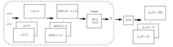
Figure 1: Block diagram of the TF-DOAnet algorithm. The dashed envelope describes the feature extraction step.

2.3 Training phase

The supervision in the training phase is based on the WDO assumption in which each TF bin is dominated by (at most) a single speaker. The training is based on simulated data generated by a publicly availble RIR generator software, efficiently implementing the image method [1]. A four microphone linear array was simulated with $(8,8,8)$ cm inter-microphones distances. Similar microphone inter-distances were used in the test phase. For each training sample, the acoustic conditions were randomly drawn from one of the simulated rooms of different sizes and different reverberation levels $\textrm{RT}_{60}$ as described in Table 1. The microphone array was randomly placed in the room in one out of six arbitrary positions.

Table 1: Configuration of training data generation. All rooms are $2.7$ m in height

Simulated training data
	Room 1	Room 2	Room 3	Room 4	Room 5
Room size	($6\times 6$) m	($5\times 4$) m	($10\times 6$ m)	($8\times 3$) m	($8\times 5$) m
$\textrm{RT}_{60}$	$0.3$ s	$0.2$ s	$0.8$ s	$0.4$ s	$0.6$ s
Signal	Noiseless signals from WSJ1 training database
Array position in room	6 arbitrary positions in each room
Source-array distance	$1.5$ m with added noise with $0.1$ variance

Table 2: Configuration of test data generation. All rooms are $3$ m in height

Simulated test data
	Room 1	Room 2
Room size	($5\times 7$) m	($9\times 4$) m
$\textrm{RT}_{60}$	$0.38$ s	$0.7$ s
Source-array distance	$1.3$ m	$1.7$ m
Signal	Noiseless signals from WSJ1 test database
Array position in room	4 arbitrary positions in each room

For each scenario, two clean signals were randomly drawn from the Wall Street Journal 1 (WSJ1) database [15] and then convolved with RIRs corresponding to two different DOAs in the range $\Theta=\{0,5,\ldots,180\}$. The sampling rate of all signals and RIRs was set to $16\text{KHz}$. The speakers were positioned in a radius of $r=1.5m$ from the center of the microphone array. To enrich the training diversity, the radius of the speakers was perturbed by a Gaussian noise with a variance of $0.1$ m. The DOA of each speaker was calculated w.r.t. the center of the microphone array.

The contributions of the two sources were then summed with a random signal to interference ratio (SIR) selected in the range of $\text{SIR}\in\left[-2,2\right]$ to obtain the received microphone signals. Next, we calculated the STFT of both the mixture and the STFT of the separate signals with a frame-length $K=512$ and an overlap of $75\%$ between two successive frames.

We then constructed the audio feature matrix ${R}$ as described in Sec. 2.1. In the training phase, both the location and a clean recording of each speaker were known, hence they could be used to generate the labels. For each TF bin $(l,k)$, the dominating speaker was determined by:

$$\mbox{dominant speaker}\leftarrow\operatornamewithlimits{argmax}_{i}|s^{i}(l,k)h_{\text{ref}}^{i}(l,k)|.$$ (8)

The ground-truth label $D_{l,k}$ is the DOA of the dominant speaker. The training set comprised four hours of recordings with 30000 different scenarios of mixtures of two speakers. It is worth noting that as the length of each speaker recording was different, the utterances could also include non-speech or single-speaker frames. The network was trained to minimize the cross-entropy between the correct and the estimated DOA. The cross-entropy cost function was summed over all the images in the training set. The network was implemented in Tensorflow with the ADAM optimizer [12]. The number of epochs was set to be 100, and the training stopped after the validation loss increased for 3 successive epochs. The mini-batch size was set to be $64$ images.

3 Experimental Study

3.1 Experimental setup

In this section we evaluate the TF-DOAnet and compare its performance to classic and DNN-based algorithms. To objectively evaluate the performance of the TF-DOAnet, we first simulated 2 unfamiliar test rooms. Then, we tested our TF-DOAnet with real RIR recordings in different rooms. Finally, a real-life scenario with fast moving speakers was recorded and tested.

subsec:experimental_setup For each test scenario, we selected two speakers from the test set of the WSJ1 database [15], placed them at two different angles between $0^{\circ}$ and $180^{\circ}$ relative to the microphone array, at a distance of either $1$m or $2$m. The signals were generated by convolving the signals with RIRs corresponding to the source positions and with either simulated or recorded acoustic scenarios.

Performance measures Two different measures to objectively evaluate the results were used: the mean absolute error (MAE) and the localization accuracy (Acc.). The MAE, computed between the true and estimated DOAs for each evaluated acoustic condition, is given by

$$\textrm{MAE}(^{\circ})=\frac{1}{N\cdot C}\sum_{c=1}^{C}\min_{\pi\in S_{N}}\sum_{n=1}^{N}|\theta_{n}^{c}-\hat{\theta}_{\pi(n)}^{c}|,$$ (9)

where $N$ is the number of simultaneously active speakers and $C$ is the total number of speech mixture segments considered for evaluation for a specific acoustic condition. In our experiments $N=2$. The true and estimated DOAs for the $n$-th speaker in the $c$-th mixture are denoted by $\theta_{n}^{c}$ and $\hat{\theta}_{n}^{c}$, respectively.

The localization accuracy is given by

$$\textrm{Acc.}(\%)=\frac{\hat{C}_{\textrm{acc.}}}{C}\times 100$$ (10)

where $\hat{C}_{\textrm{acc.}}$ denotes the number of speech mixtures for which the localization of the speakers is accurate. We considered the localization of speakers for a speech frame to be accurate if the distance between the true and the estimated DOA for all the speakers was less than or equal to $5^{\circ}$.

Compared algorithms We compared the performance of the TF-DOAnet with two frequently used baseline methods, namely the MUSIC and SRP-PHAT algorithms. In addition, we compared its performance with the CNN multi-speaker DOA (CMS-DOA) estimator [4]. To facilitate the comparison, the MUSIC pseudo-spectrum was computed for each frequency sub-band and for each STFT time frame, with an angular resolution of $5^{\circ}$ over the entire DOA domain. Then, it was averaged over all frequency subbands to obtain a broadband pseudo-spectrum followed by averaging over all the time frames $L$. Next, the two DOAs with the highest values were selected as the final DOA estimates. Similar post-processing was applied to the computed SRP-PHAT pseudo-likelihood for each time frame.

3.2 Speaker localization results

Static simulated scenario

We first generated a test dataset with simulated RIRs. Two different rooms were used, as described in Table 2. For each scenario, two speakers (male or female) were randomly drawn from the WSJ1 test database, and placed at two different DOAs within the range $\{0,5,\ldots,180\}$ relative to the microphone array. The microphone array was similar to the one used in the training phase. Using the RIR generator, we generated the RIR for the given scenario and convolved it with the speakers’ signals.

The results for the TF-DOAnet compared with the competing methods are depicted in Table 3. The tables shows that the deep-learning approaches outperformed the classic approaches. The TF-DOAnet achieved very high scores and outperformed the DNN-based CMS-DOA algorithm in terms of both MAE and accuracy.

Static real recordings scenario

The best way to evaluate the capabilities of the TF-DOAnet is testing it with real-life scenarios. For this purpose, we first carried out experiments with real measured RIRs from a multi-channel impulse response database [11]. The database comprises RIRs measured in an acoustics lab for three different reverberation times of $\textrm{RT}_{60}=0.160,0.360$, and $0.610$ s. The lab dimensions are $6\times 6\times 2.4$ m.

The recordings were carried out with different DOA positions in the range of $[0^{\circ},180^{\circ}]$, in steps of $15^{\circ}$. The sources were positioned at distances of $1$ m and $2$ m from the center of the microphone array. The recordings were carried out with a linear microphone array consisting of $8$ microphones with three different microphone spacings. For our experiment, we chose the [8, 8, 8, 8, 8, 8, 8] cm setup. In order to construct an array setup identical to the one in the training phase, we selected a sub-array of the four center microphones out of the total 8 microphones in the original setup. Consequently, we used a uniform linear array (ULA) with $M=4$ elements with an inter-microphone distance of $8$ cm.

The results for the TF-DOAnet compared with the competing methods are depicted in Table 4. Again, the TF-DOAnet outperforms all competing methods, including the CMS-DOA algorithm. Interestingly, for the 1 m case, the best results for the TF-DOAnet were obtained for the highest reverberation level, namely $\textrm{RT}_{60}=610$ ms, and for the 2 m case, for $\textrm{RT}_{60}=360$ ms. While surprising at first glance, this can be explained using the following arguments. There is an accumulated evidence that reverberation, if properly addressed, can be beneficial in speech processing, specifically for multi-microphone speech enhancement and source extraction [10, 14, 8] and for speaker localization [6, 13]. In reverberant environments, the intricate acoustic propagation pattern constitutes a specific “fingerprint” characterizing the location of the speaker(s). When reverberation level increases, this fingerprint becomes more pronounced and is actually more informative than its an-echoic counterpart. An inference methodology that is capable of extracting the essential driving parameters of the RIR will therefore improve when the reverberation is higher. If the acoustic propagation becomes even more complex, as is the case of high reverberation and a remote speaker, a slight performance degradation may occur, but as evident from the localization results, for sources located 2 m from the array, the performance for $\textrm{RT}_{60}=610$ ms was still better than the performance for $\textrm{RT}_{60}=160$ ms.

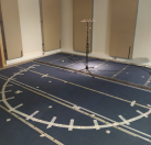
(a) Room view.

(b) Speakers’ trajectory.

Figure 2: Real-life experiment setup.

Real-life dynamic scenario

To further evaluate the capabilities of the TF-DOAnet, we also carried out real dynamic scenarios experiments. The room dimensions are $6\times 6\times 2.4$ m. The room reverberation level can be adjusted and we set the $\textrm{RT}_{60}$ at two levels, $390$ ms and $720$ ms, respectively. The microphone array consisted of $4$ microphones with an inter-microphone spacing of $8$ cm. The speakers walked naturally on an arc at a distance of about $2.2$ m from the center of the microphone array. For each $\textrm{RT}_{60}$ two experiments were recorded. The two speakers started at the angles $20^{\circ}$ and $160^{\circ}$ and walked until they reached $70^{\circ}$ and $100^{\circ}$, respectively, turned around and walked back to their starting point. This was done several times throughout the recording. Figure 2(a) depicts the real-life experiment setup and Fig. 2(b) depicts a schematic diagram of the setup of this experiment. The ground truth labels of this experiment were measured with the Marvelmind indoor 3D tracking set.

Figures 4 and 4 depict the results of the two experiments. It is clear that the TF-DOAnet outperformed the CMS-DOA algorithm, especially for the high RT₆₀ conditions. Whereas the CMS-DOA fluctuated rapidly, the TF-DOAnet output trajectory was smooth and noiseless.

(a) Ground truth.

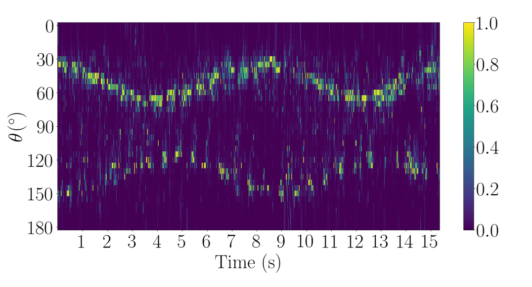
(b) CMS-DOA.

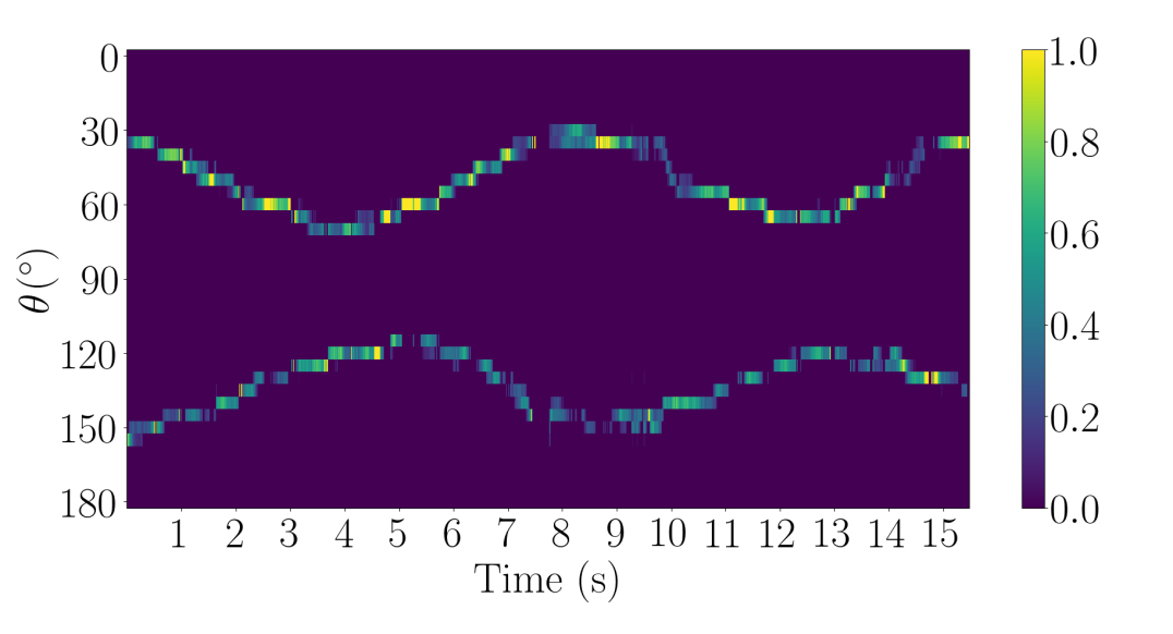
(c) The TF-DOAnet.

Figure 3: Real-life recording of two moving speakers in a $6\times 6\times 2.4$ room with RT${}_{60}=390$ ms.

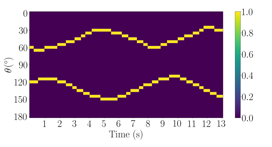
(d) Ground truth.

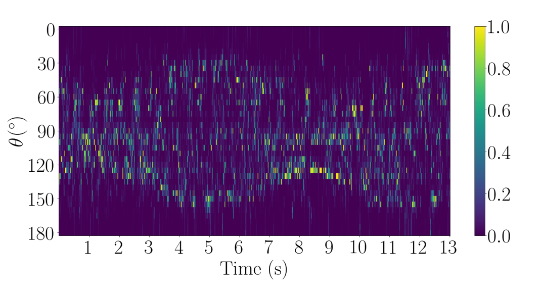
(e) CMS-DOA.

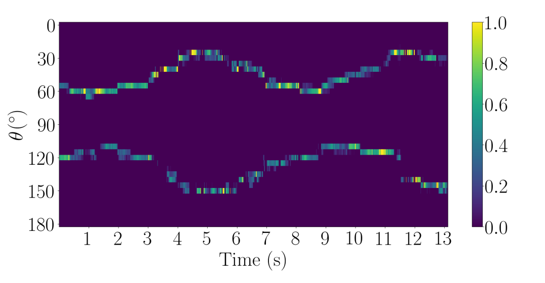
(f) The TF-DOAnet.

Figure 4: Real-life recording of two moving speakers in a $6\times 6\times 2.4$ room with RT${}_{60}=720$ ms.

Table 3: Results for two different test rooms with simulated RIRs

Test Room	Room 1		Room 2
Measure	MAE	Acc.	MAE	Acc.
MUSIC [7]	26.2	28.4	31.5	16.9
SRP-PHAT [2]	25.1	26.7	35.0	15.6
CMS-DOA [4]	13.1	71.1	24.0	38.1
TF-DOAnet	0.3	99.5	1.7	94.3

Table 4: Results for three different rooms at distances of $1$ m and $2$ m with measured RIRs

Distance	$1$ m						$2$ m
$\textrm{RT}_{60}$	0.160 s		0.360 s		0.610 s		0.160 s		0.360 s		0.610 s
Measure	MAE	Acc.	MAE	Acc.	MAE	Acc.	MAE	Acc.	MAE	Acc.	MAE	Acc.
MUSIC	18.7	57.6	19.2	53.2	21.9	42.9	18.4	54.1	26.1	35.8	25.4	32.2
SRP-PHAT	9.0	39.0	13.9	39.4	18.6	29.9	9.7	36.0	16.5	24.7	27.7	21.3
CMS-DOA	1.6	76.3	7.3	75.2	8.4	71.9	5.1	79.5	9.7	60.1	17.5	40.0
TF-DOAnet	1.3	97.5	3.5	83.5	0.9	98.3	5.0	89.5	1.7	95.7	4.8	84.2

3.3 Ablation study

In our implementation, we used the real and imaginary part of the RTF (4). Other approaches might be beneficial. For example, in [5], the $\cos$ and the $\sin$ of the phase of the RTF were used. In other approaches, the spectrum was added to the spatial features [25].

In this section, the different features were tested with the same model. We compared the proposed features with two other features. First, we used the proposed features as described in (4). The second approach was a variant of our approach with the spectrum added (‘TF-DOAnet with Spec.’). The third, used the $\cos$ and the $\sin$ features as presented in [5] (‘Cos-Sin’). All features were crafted from the same training data described in Sec. 2.3. We tested the different approaches in the test conditions described in 2.

First, it is clear that all the features with our high resolution TF model outperformed the frame-based CMS-DOA algorithm, as reported in Table 3. This confirms that the TF supervision is beneficial for the task at hand. Second, the proposed features were shown to be better than the Cos-Sin features. Finally, it is very interesting to note that the addition of the spectrum features slightly deteriorated the results for this task.

Table 5: Ablation study results with different features

Test Room	Room 1		Room 2
Measure	MAE	Acc.	MAE	Acc.
Cos-Sin	1.2	96.1	2.8	91.3
TF-DOAnet with Spec.	0.6	98.4	3.3	86.7
TF-DOAnet	0.3	99.5	1.7	94.3

4 Conclusions

A FCN approach was presented in this paper for the DOA estimation task. Instantaneous RTF features were used to train the model. The high TF resolution facilitated the tracking of multiple moving speakers simultaneously. A comprehensive experimental study was carried out with simulated and real-life recordings. The proposed approach outperformed both the classic and CNN-based SOTA algorithms in all experiments. Training and test datasets which represent different real-life scenarios were constructed as a DOA benchmark and will become available after publication.

Broader impact

Several modern technologies can benefit from the proposed localization algorithm. We already mentioned the emerging technology of smart speakers in the Introduction. These devices are equipped with multiple microphones and are implementing location-specific tasks, e.g. the extraction of the speaker of interest. Of particular interest are socially assistive robots (SARs), as they are likely to play an important role in healthcare and psychological well-being, in particular during non-medical phases inherent to any hospital process.

The algorithm neither uses the content nor the identity of the speakers and hence does not to violate the privacy of the users. Moreover, since normally speech signal cannot propagate over long distances, the algorithm application is limited to small enclosures.

References

- [1] Jont B. Allen and David A. Berkley. Image method for efficiently simulating small-room acoustics. The Journal of the Acoustical Society of America, 65(4):943–950, 1979.
- [2] Michael S. Brandstein and Harvey F. Silverman. A robust method for speech signal time-delay estimation in reverberant rooms. In IEEE International Conference on Acoustics, Speech and Signal Processing (ICASSP), 1997.
- [3] Soumitro Chakrabarty and Emanuël A. P. Habets. Broadband DOA estimation using convolutional neural networks trained with noise signals. IEEE Workshop on Applications of Signal Processing to Audio and Acoustics (WASPAA), 2017.
- [4] Soumitro Chakrabarty and Emanuël A. P. Habets. Multi-speaker DOA estimation using deep convolutional networks trained with noise signals. IEEE Journal of Selected Topics in Signal Processing, 13(1):8–21, 2019.
- [5] Shlomo E. Chazan, Hodaya Hammer, Gershon Hazan, Jacob Goldberger, and Sharon Gannot. Multi-microphone speaker separation based on deep DOA estimation. In European Signal Processing Conference (EUSIPCO), 2019.
- [6] Antoine Deleforge, Florence Forbes, and Radu Horaud. Acoustic space learning for sound-source separation and localization on binaural manifolds. International journal of neural systems, 25(01):1440003, 2015.
- [7] Jacek P. Dmochowski, Jacob Benesty, and Sofiene Affes. Broadband music: Opportunities and challenges for multiple source localization. In Proc. IEEE Workshop on Applications of Signal Processing to Audio and Acoustics (WASPAA), 2007.
- [8] Ivan Dokmanić, Robin Scheibler, and Martin Vetterli. Raking the cocktail party. IEEE journal of selected topics in signal processing, 9(5):825–836, 2015.
- [9] Christine Evers, Heinrich Loellmann, Heinrich Mellmann, Alexander Schmidt, Hendrik Barfuss, Patrick Naylor, and Walter Kellermann. The locata challenge: Acoustic source localization and tracking. arXiv preprint arXiv:1909.01008, 2019.
- [10] Sharon Gannot, David Burshtein, and Ehud Weinstein. Signal enhancement using beamforming and nonstationarity with applications to speech. IEEE Transactions on Signal Processing, 49(8):1614–1626, 2001.
- [11] Elior Hadad, Florian Heese, Peter Vary, and Sharon Gannot. Multichannel audio database in various acoustic environments. In International Workshop on Acoustic Signal Enhancement (IWAENC), 2014.
- [12] Diederik P Kingma and Jimmy Ba. Adam: A method for stochastic optimization. arXiv preprint arXiv:1412.6980, 2014.
- [13] Bracha Laufer-Goldshtein, Ronen Talmon, and Sharon Gannot. Semi-supervised sound source localization based on manifold regularization. IEEE/ACM Transactions on Audio, Speech, and Language Processing, 24(8):1393–1407, 2016.
- [14] Shmulik Markovich-Golan, Sharon Gannot, and Israel Cohen. Multichannel eigenspace beamforming in a reverberant noisy environment with multiple interfering speech signals. IEEE Tran. on Audio, Speech, and Language Processing, 17(6):1071–1086, August 2009.
- [15] Douglas B. Paul and Janet M. Baker. The design for the Wall Street Journal-based CSR corpus. In Workshop on Speech and Natural Language, 1992.
- [16] Hadrien Pujol, Eric Bavu, and Alexandre Garcia. Source localization in reverberant rooms using deep learning and microphone arrays. In International Congress on Acoustics (ICA), 2019.
- [17] Scott Rickard and Ozgiir Yilmaz. On the approximate w-disjoint orthogonality of speech. In IEEE International Conference on Acoustics, Speech, and Signal Processing (ICASSP), 2002.
- [18] Olaf Ronneberger, Philipp Fischer, and Thomas Brox. U-net: Convolutional networks for biomedical image segmentation. In International Conference on Medical image computing and computer-assisted intervention, 2015.
- [19] Ralph Schmidt. Multiple emitter location and signal parameter estimation. IEEE Transactions on Antennas and Propagation, 34(3):276–280, 1986.
- [20] Sebastian Stenzel, Jürgen Freudenberger, and Gerhard Schmidt. A minimum variance beamformer for spatially distributed microphones using a soft reference selection. In Joint Workshop on Hands-free Speech Communication and Microphone Arrays (HSCMA), 2014.
- [21] Ryu Takeda and Kazunori Komatani. Discriminative multiple sound source localization based on deep neural networks using independent location model. IEEE Spoken Language Technology Workshop (SLT), 2016.
- [22] Juan Manuel Vera-Diaz, Daniel Pizarro, and Javier Macias-Guarasa. Towards end-to-end acoustic localization using deep learning: From audio signals to source position coordinates. Sensors, 18(10):3418, 2018.
- [23] Fabio Vesperini, Paolo Vecchiotti, Emanuele Principi, Stefano Squartini, and Francesco Piazza. A neural network based algorithm for speaker localization in a multi-room environment. In IEEE International Workshop on Machine Learning for Signal Processing (MLSP), 2016.
- [24] DeLiang Wang and Jitong Chen. Supervised speech separation based on deep learning: An overview. IEEE/ACM Transactions on Audio, Speech, and Language Processing, 26(10):1702–1726, 2018.
- [25] Zhong-Qiu Wang, Jonathan Le Roux, and John R. Hershey. Multi-channel deep clustering: Discriminative spectral and spatial embeddings for speaker-independent speech separation. In IEEE International Conference on Acoustics, Speech and Signal Processing (ICASSP), 2018.
- [26] Xiong Xiao, Shengkui Zhao, Xionghu Zhong, Douglas L Jones, Eng Siong Chng, and Haizhou Li. A learning-based approach to direction of arrival estimation in noisy and reverberant environments. In IEEE International Conference on Acoustics, Speech and Signal Processing (ICASSP), 2015.
- [27] Ozgur Yilmaz and Scott Rickard. Blind separation of speech mixtures via time-frequency masking. IEEE Transactions on Signal Processing, 52(7):1830–1847, 2004.