Exploring the Design Space of Static and Incremental Graph Connectivity Algorithms on GPUs

Changwan Hong MIT CSAIL changwan@mit.edu , Laxman Dhulipala CMU ldhulipa@andrew.cmu.edu and Julian Shun MIT CSAIL jshun@mit.edu

Abstract.

Connected components and spanning forest are fundamental graph algorithms due to their use in many important applications, such as graph clustering and image segmentation. GPUs are an ideal platform for graph algorithms due to their high peak performance and memory bandwidth. While there exist several GPU connectivity algorithms in the literature, many design choices have not yet been explored. In this paper, we explore various design choices in GPU connectivity algorithms, including sampling, linking, and tree compression, for both the static as well as the incremental setting. Our various design choices lead to over 300 new GPU implementations of connectivity, many of which outperform state-of-the-art. We present an experimental evaluation, and show that we achieve an average speedup of 2.47x speedup over existing static algorithms. In the incremental setting, we achieve a throughput of up to 48.23 billion edges per second. Compared to state-of-the-art CPU implementations on a 72-core machine, we achieve a speedup of 8.26–14.51x for static connectivity and 1.85–13.36x for incremental connectivity using a Tesla V100 GPU.

Connected components, Graph algorithms, GPU algorithms, Spanning forest

^†^†ccs: Theory of computation Parallel algorithms

1. Introduction

Connected components (connectivity) is a fundamental graph problem that plays a critical role in many graph applications. Given an undirected graph with $n$ vertices and $m$ edges, the problem assigns each vertex a label such that vertices that are reachable from each other have the same label, and otherwise have different labels (Cormen et al., 2009). Connectivity algorithms are used in many applications, such as computer vision (Elhamifar and Vidal, 2013; Ho et al., 2003), VLSI design (Li and Behjat, 2006), and social analysis (Haythornthwaite, 2005). Graph connectivity is also a key subroutine to solve other graph algorithms, such as biconnectivity (Tarjan and Vishkin, 1985) and clustering (Ester et al., 1996; Patwary et al., 2012a; Wen et al., 2017; Xu et al., 2007), and some of these algorithms require many calls to graph connectivity. As such, there has been a large amount of work on efficient parallel connectivity algorithms (Awerbuch and Shiloach, 1987; Chin et al., 1982; Chong and Lam, 1995; Cole and Vishkin, 1991; Han and Wagner, 1990; Hirschberg et al., 1979; Iwama and Kambayashi, 1994; Johnson and Metaxas, 1997; Karger et al., 1999; Koubek and Krsnakova, 1985; Kruskal et al., 1990; Nath and Maheshwari, 1982; Phillips, 1989; Reif, 1985; Shiloach and Vishkin, 1982; Gazit, 1991; Vishkin, 1984; Shun et al., 2014; Dhulipala et al., 2018; Greiner, 1994; Halperin and Zwick, 1994; Slota et al., 2014; Blelloch et al., 2012; Bader et al., 2005; Bader and JaJa, 1996; Madduri and Bader, 2009; Bader and Cong, 2005; Bus and Tvrdik, 2001; Caceres et al., 2004; Patwary et al., 2012b; Hambrusch and TeWinkel, 1988; Hsu et al., 1997; Nguyen et al., 2013a; Hawick et al., 2010; Soman et al., 2010; Banerjee and Kothapalli, 2011; Shun and Blelloch, 2013; Sutton et al., 2018; Liu and Tarjan, 2019; Stergiou et al., 2018; Jain et al., 2017; Kiveris et al., 2014; Iverson et al., 2015; Chitnis et al., 2013; Andoni et al., 2018; Behnezhad et al., 2019b, a).

Graphics processing units (GPUs) are attractive devices for performing graph computations because of their high computing power and memory bandwidth. However, achieving high performance using GPUs is challenging due to several factors, including uncoalesced memory access, insufficient parallelism to tolerate high memory latency, load imbalance, and thread divergence. Several GPU connectivity implementations have been proposed in the literature (Pai and Pingali, 2016; Ben-Nun et al., 2017; Wang et al., 2016; Meng et al., 2019; Cong and Muzio, 2014; Jaiganesh and Burtscher, 2018; Sutton et al., 2018), but we found that there are many algorithmic choices and optimizations that have not been thoroughly explored for GPU connectivity. The goal of this paper is to explore this large design space to better understand how different choices affect performance.

In this paper, we study min-based connectivity algorithms (Jayanti and Tarjan, 2016; Jayanti et al., 2019; Patwary et al., 2012b; Liu and Tarjan, 2019; Stergiou et al., 2018; Shun and Blelloch, 2013), which are based on vertices propagating labels to other connected vertices, and keeping the minimum label received. At convergence, vertices will have the same label if and only if they are in the same connected component. A large number of our algorithms are based on using a union-find data structure for maintaining disjoint sets. The data structure maintains a tree for each sub-component found so far, and joins trees to merge sub-components that are connected. We also study several other min-based algorithms that maintain trees, but not using a disjoint set data structure. All existing GPU connectivity implementations are min-based; however, there are various design choices that have not been explored, such as different rules for searching and compressing union-find trees and for propagating labels. Furthermore, these algorithms can be improved by using sampling as a preprocessing step to remove vertices in a large component from consideration, so that the remaining steps are more efficient. Sutton et al. (Sutton et al., 2018) provide one instantiation of sampling combined with a particular union-find algorithm. Inspired by their work, we explore different sampling strategies in this paper, and combine them with each of our algorithms to sweep the search space.

To implement different connectivity algorithms, we designed the $\mathsf{GConn}$ framework, which is an extension of the $\mathsf{ConnectIt}$ framework (Dhulipala et al., 2020b) for multicore CPUs. However, achieving high performance for connectivity algorithms on GPUs requires significant effort beyond what is provided in $\mathsf{ConnectIt}$ for two reasons. The first reason is that the programming models on CPUs and GPUs are different, which required us to significantly rewrite the codebase. The second reason is that the bottlenecks on CPUs and GPUs are different (e.g., on GPUs, performance can be easily degraded from uncoalesced memory accesses, low parallelism, and heavy use of atomics), and this required us to apply GPU-specific optimizations to achieve high performance. $\mathsf{GConn}$ contains several GPU-specific optimizations: edge reorganization, which is specific to our connectivity algorithms, and CSR coalescing and vertex gathering, which are commonly used in other graph algorithms.

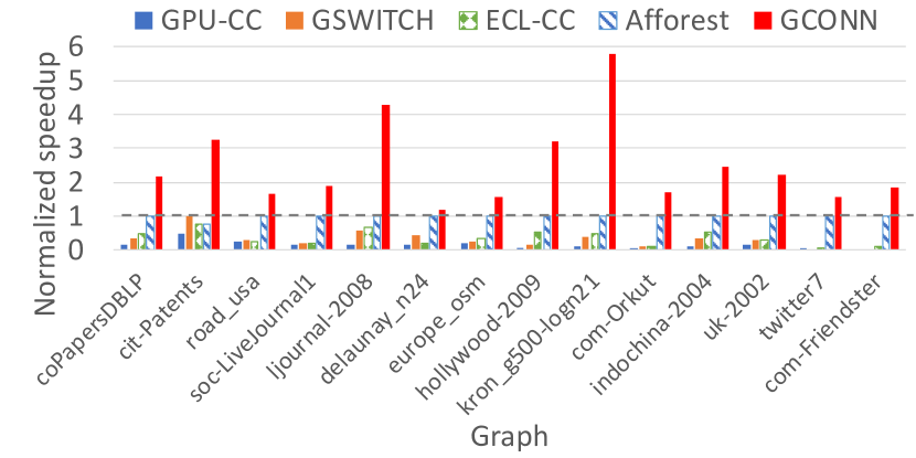
In this paper, we generate a total of 339 different connectivity implementations and evaluate their performance. With our comprehensive study, we are able to obtain the fastest GPU connectivity algorithms to date. Figure 1 shows the normalized performance of the fastest implementation in $\mathsf{GConn}$ compared to four state-of-the-art GPU implementations: $\mathsf{GPU\mathchar 45\relax CC}$ (Soman et al., 2010), $\mathsf{GSWITCH}$ (Meng et al., 2019), $\mathsf{ECL\mathchar 45\relax CC}$ (Jaiganesh and Burtscher, 2018), and $\mathsf{Afforest}$ (Sutton et al., 2018). We achieve an average speedup of 2.48x over the fastest implementation for each graph input. Although we consider many connectivity implementations, we note that based on the results of our experimental study, practitioners only need to consider a handful of these implementations to obtain high performance.

Refer to caption — Figure 1. Normalized speedup of four existing implementations/libraries and $\mathsf{GConn}$ . The fastest existing implementation’s performance is normalized to 1.

In addition to connected components, most of our algorithms solve the related problem of computing a spanning forest of a graph. Furthermore, we extend our algorithms to the incremental setting, where the connected components or spanning forest is updated upon new edge arrivals. Our incremental algorithms are able to achieve throughputs of up to 48.23 billion edges per second, which improves upon state-of-the-art for GPUs— $\mathsf{EvoGraph}$ (Sengupta and Song, 2017)—by orders of magnitude based on a rough comparison of reported numbers since their code is not available. Additionally, we compare our GPU implementations to the CPU implementations in $\mathsf{ConnectIt}$ on a 72-core CPU and show that we achieve speedups of 8.27–17.48x for static connectivity, and 1.85–13.36x for incremental connectivity on a Tesla V100 GPU that costs about half as much as the CPU. Finally, we perform an analysis of different design choices to explain where the performance benefits of our fastest implementations are coming from. $\mathsf{GConn}$ is publicly available at https://github.com/hochawa/gconn.

Summary of Contributions. We believe that this paper presents the most comprehensive study of GPU implementations of connectivity for both static and incremental connectivity to date. By performing this extensive study, we provide an understanding of how different algorithmic choices affect performance and where the performance benefits of fast connectivity implementations come from. Our paper provides the fastest GPU implementations of connectivity, which we obtain by combining many combinations of algorithmic choices that prior work did not explore. Building high-performance implementations of these optimizations and combining them is key to achieving high performance. We believe that our proposed techniques can be integrated into graph processing compilers and other frameworks to significantly improve performance.

The remainder of the paper is organized as follows. Section 2 discusses graph terminology and prior work. Section 3 describes the design choices in $\mathsf{GConn}$ , and their relation to prior work. We perform a comprehensive evaluation of our implementations in Section 4, and conclude in Section 5.

2. Notation, Preliminaries, and Prior Work

Graph Notation and Formats. In this paper, we focus on undirected, unweighted graphs, which we denote as $G=(V,E)$ . $V$ and $E$ are the set of vertices and edges, and $n=|V|$ and $m=|E|$ are the number of vertices and edges, respectively. We consider two graph formats, coordinate list (COO) and compressed sparse row (CSR), with 0-based index notation (i.e., each vertex is labeled with a unique identifier in the range $[0,\ldots,n-1]$ ). The COO format is represented using an array of edges, where each edge contains a source and a destination vertex. The CSR format contains two arrays, $\mathit{Offsets}$ and $\mathit{Edges}$ , of lengths $n+1$ and $m$ , respectively. The edges for vertex $i$ are stored in $\mathit{Offsets}[i],\ldots,\mathit{Offsets}[i+1]-1$ , and $\mathit{Offsets}[n]=m$ , and we assume they are in sorted order.

Graph Connectivity Problems. A connected component (CC) in $G$ is a maximal set of vertices in which each pair of vertices in the component is connected by a path. A connected components algorithm computes a vertex label $\mathit{labels}(v)$ for each $v\in V$ . Two vertices $u,v\in V$ are in the same component if and only if $\mathit{labels}(u)=\mathit{labels}(v)$ . A connectivity query returns true if and only if two input vertices belong to the same component. A spanning forest (SF) maintains a connected tree for each connected component. A breadth-first search (BFS) takes a graph with a source vertex and returns an array $A$ where $A(v)$ stores the shortest path between the source and $v$ . If a vertex $v$ is unreachable from the source vertex, $A(v)$ is set to infinity.

A union-find (disjoint set) data structure keeps track of a number of disjoint sets such that elements in each set have the same labels. Each set is represented by a tree and each element in the set has a parent pointer. The parent of a tree root points to itself. In this paper, we assume that elements either point to themselves or point to a parent with a smaller ID. The data structure provides three operations: MakeSet, Union, and Find (Cormen et al., 2009). MakeSet( $u$ ) generates a new tree that is composed of only one node $u$ , which is a root. Union( $u,v$ ) joins two trees, $u$ and $v$ , into a single tree. Find( $u$ ) returns the label of the root of the tree containing $u$ . Find and Union operations can perform path compression during execution to speed up subsequent operations. Union-find can be used for connectivity by creating a set for each vertex, and calling Union on the endpoints of each edge. The labels of the vertices can be obtained in the end by running Find on each vertex.

In this paper, we also consider connectivity algorithms that maintain trees, where we can move vertices between trees without completely joining the trees (as needed for merging sets in union-find). We refer to an algorithm as root-based if it only modifies the parent pointers of tree roots to point to vertices in other trees (vertices are still free to update their pointer to point to other vertices in the same tree). All of the union-find algorithms are root-based.

Compare-and-Swap. In this paper, we use the atomic compare-and-swap (CAS) primitive, which takes as input a memory location, an old value, and a new value. If the value stored in the memory location is equal to the old value, then the CAS atomically replaces the old value with the new value, and returns true. Otherwise, the CAS does not update the value, and returns false.

Prior work on GPUs. Soman et al. (Soman et al., 2010) provide GPU-CC, the first high-performance implementation of the Shiloach-Vishkin algorithm (Shiloach and Vishkin, 1982) on GPUs. Many libraries (e.g., $\mathsf{Gunrock}$ (Wang et al., 2017), $\mathsf{IrGL}$ (Pai and Pingali, 2016), and $\mathsf{Groute}$ (Ben-Nun et al., 2017)) also adopt a variant of this approach. Note that $\mathsf{GPU\mathchar 45\relax CC}$ uses the COO format so the performance does not suffer from poor load-balance on GPUs. GSWITCH (Meng et al., 2019) is a framework for graph processing which provides different combinations of optimization strategies for different graph algorithms, including connectivity. Hence, $\mathsf{GSWITCH}$ allows tens of different combinations of optimizations (e.g., different load-balancing strategies can be combined with other optimization strategies). The best set of optimizations is found using a machine learning approach. ECL-CC (Jaiganesh and Burtscher, 2018) uses a concurrent union-find algorithm for connectivity in the CSR format. Afforest (Sutton et al., 2018) incorporates the $k$ -out sampling strategy (described in Section 3.3) that significantly improves performance on many real-world graphs. $\mathsf{Afforest}$ uses the CSR format, and uses the load-balancing technique from (Ben-Nun et al., 2017).

3. $\mathsf{GConn}$ Overview

We first describe the overview of $\mathsf{ConnectIt}$ in Section 3.1. Then we provide an overview of the $\mathsf{GConn}$ framework in Section 3.2. In Sections 3.3 and 3.4, we provide an overview of specific algorithmic choices that we explore.

3.1. Overview of $\mathsf{ConnectIt}$

$\mathsf{ConnectIt}$ is a framework for multicore connectivity algorithms that outperforms existing state-of-the-art multicore algorithms and generates various implementations for connectivity based on a two-phase execution model: a sampling phase and a finish phase. In the sampling phase, a subset of edges are inspected to partially form connected components. Next, the most frequently occurring label ( $L_{\max}$ ) is identified. In the finish phase, only vertices whose label is not equal to $L_{\max}$ need to process their outgoing edges. Vertices with label $L_{\max}$ skip processing their edges, since any neighbor with label $L_{\max}$ is already in the same component, and any neighbor with label other than $L_{\max}$ will process an edge to this vertex. This two-phase execution can significantly reduce the number of edges processed. $\mathsf{ConnectIt}$ provides correctness proofs for the two-phase execution. $\mathsf{GConn}$ is an extension of $\mathsf{ConnectIt}$ that we developed for GPUs, which enables easy exploration of different algorithmic choices.

3.2. $\mathsf{GConn}$ Framework

In this section, we give an overview of the $\mathsf{GConn}$ that we use to obtain our GPU implementations for static connectivity, spanning forest, and incremental connectivity.

Algorithm 1

\mathsf{GConn}

for Static Connectivity

1:procedure StaticConn(

G(V,E),\mathit{sample},\mathit{finish},\mathit{compress}

)

\mathit{labels}\leftarrow\textsc{InitLabel}(V)

\mathit{labels}\leftarrow\textsc{SamplePhase}(G,\mathit{labels},\mathit{sample},\mathit{finish},\mathit{compress})

L_{\max}\leftarrow\textsc{GetMostFrequentLabel}(\mathit{labels})

\mathit{labels}\leftarrow\textsc{FinishPhase}(G,\mathit{labels},\mathit{finish},\mathit{comp})

\mathit{labels}\leftarrow\textsc{LabelFinalization}(V,\mathit{labels})

7: return

\mathit{labels}

Static Connectivity. Algorithm 1 presents the main steps in $\mathsf{GConn}$ . $\mathsf{GConn}$ takes in a graph in either CSR or COO format, as well as parameters for the sampling algorithm (sample), the finish algorithm (finish), and the compression algorithm (compress). The label of each vertex is initialized to its own ID on Line 2, and the sampling phase is performed on Line 3. On Line 4, the most frequently occurring label ( $L_{\max}$ ) is identified from the result of the sampling phase. On Line 5, $\mathsf{GConn}$ performs the finish phase, processing edges of vertices with label not equal to $L_{\max}$ . Finally, on Line 6, we finalize the labels of each vertex by assigning each vertex the label of the root of its tree. We use C++ templates and inlined functions to achieve high-performance implementations while keeping the $\mathsf{GConn}$ implementations high-level. Our implementations modularize the routines for the sampling algorithm, finish algorithm, compression algorithm, the load-balancing strategy, and graph format, making it easy to test different implementations and add new variants.

Algorithm 2

\mathsf{GConn}

for Spanning Forest

1:procedure SpanningForest(

G(V,E),\mathit{sample},\mathit{finish},\mathit{compress}

)

\mathit{labels}\leftarrow\textsc{InitLabel}(V)

\mathit{edges}\leftarrow\textsc{InitEdge}(V)

\mathit{(labels,edges)}\leftarrow\textsc{SamplePhase}(G,\mathit{labels},\mathit{sample},\mathit{finish},\mathit{compress})

L_{\max}\leftarrow\textsc{GetMostFrequentLabel}(\mathit{labels})

\mathit{(labels,edges)}\leftarrow\textsc{FinishPhase}(G,\mathit{labels},\mathit{finish},\mathit{comp})

7: return

\mathit{edges}

Static Spanning Forest. As shown in Algorithm 2, implementations for spanning forest are similar to those for connectivity; $\mathsf{GConn}$ supports different combinations of sampling and finish methods while generating correct spanning forest algorithms. In conjunction with the label initialization (Line 2), we also maintain the edges in the spanning forest using an auxiliary array of size $n$ (Line 3). The key idea behind our implementations of spanning forest is to assign each edge of the discovered spanning forest to a unique vertex that is one of the endpoints of the edge. This special vertex is the root vertex in the union-find structure that updates its parent pointer to point to another vertex, so that it is no longer a root. Hence, the root-based algorithms for connectivity (to be described in Section 3.4) can be converted to compute spanning forests. The sampling phase simply creates a subset of the edges for the spanning forest (Line 4), while computing partially connected components and determining $L_{\max}$ , as in static connectivity (Line 5). After that, using $L_{\max}$ , the finish phase computes the rest of the edges for the spanning forest (Line 6). The finalization step is not required for spanning forest since the edges of the spanning forest have already been generated in previous steps, which eliminates the overhead for the post-processing. In our experiments, we found that spanning forest algorithms are 6% faster on average than their static connectivity counterpart.

Incremental Connectivity. As many real-world graphs are being updated frequently, many connectivity algorithms have been proposed for dynamic graphs (McColl et al., 2013; Ediger et al., 2012; Simsiri et al., 2017; Sengupta and Song, 2017; Acar et al., 2019; Dhulipala et al., 2020a). Many of our algorithms are a natural fit for the incremental setting, where edges are inserted but not deleted. We designed $\mathsf{GConn}$ to support incremental connectivity (and spanning forest) algorithms that receive batches of operations consisting of edge insertions and connectivity queries that can be executed in parallel. We will describe how $\mathsf{GConn}$ supports incremental connectivity algorithms in Section 3.6.

3.3. Sampling Algorithms

As done in $\mathsf{ConnectIt}$ (Dhulipala et al., 2020b), we decompose connectivity algorithms into the sampling and finish phases. The sampling phase traverses a subset of edges in the graph to update the labels of vertices. The sampling phase can reduce the number of edges inspected in the finish phase, since in practice we expect that a large fraction of the vertices will already be settled in the $L_{\max}$ component after applying the sampling phase. All connectivity algorithms in the literature today, except for $\mathsf{Afforest}$ (Sutton et al., 2018), only support a finish phase. We implement sampling for graphs in CSR format due to the ease of skipping over all edges for particular vertices (i.e., the ones with label $L_{\max}$ after sampling). Below we introduce the different sampling methods implemented in $\mathsf{GConn}$ . We discuss them in the context of connectivity, although they are used similarly in spanning forest. Pseudocode for these methods can be found in the Appendix.

$k$ -out Sampling. Given a parameter $k$ , $k$ -out sampling computes connected components on a sampled graph constructed by uniformly sampling $k$ edges out of each vertex (Holm et al., 2019). Sutton et al. (Sutton et al., 2018) use a type of $k$ -out sampling strategy where the first $k$ edges out of each vertex are used. The vertices obtain labels as a result of running a parallel connected components algorithm on the sampled graph. In practice, after applying $k$ -out sampling, many of the vertices in the largest connected component will have the same label, since many real-world graphs have a single massive component that most vertices will be a part of in the sampled graph. In $\mathsf{GConn}$ , we implemented several variants of $k$ -out sampling for different values of $k$ , and found that taking the first 2 edges, as in (Sutton et al., 2018), gave the best performance overall. Taking the first 2 edges per vertex enabled us to label most of the vertices in the largest component with the final label, and minimized the overall number of edge inspections during the sampling and finish phases. Moreover, since in many real-world graphs, the edges for a vertex are sorted and if all vertices choose their first two edges (neighbors), there are likely to be many shared neighbors, which improves locality and increases the size of the large component found. For running connectivity on the subgraph, we use different variants of union-find (discussed in Section 3.4).

Hook-Based Search (HB) Sampling. Inspired by $\mathsf{ECL\mathchar 45\relax CC}$ (Jaiganesh and Burtscher, 2018), we designed the hook-based search (HB) sampling approach to potentially reduce the number of edge traversals compared to $k$ -out sampling. This approach uses a union-find structure to maintain vertex labels. First, each vertex $v$ inspects its smallest (i.e., first) neighbor $w$ , and updates its label to $\mathit{labels}(v)=\min(\mathit{labels}(v),\mathit{labels}(w))$ . This step is efficient since there is no contention. Second, for all vertices that are still roots (i.e., $\mathit{labels}(v)=v$ ), we inspect their first $N$ edges and apply the union operation to these edges. The goal of these steps is to minimize the total number of roots after sampling, since fewer roots mean that the graph is more connected. This approach can potentially require fewer edge traversals than $k$ -out sampling for $k\geq 2$ if there are few roots after the first step.

Breadth-First Search (BFS) Sampling. In breadth-first search (BFS) sampling, we run a BFS from a chosen source vertex, which discovers the connected component of this source. If the graph has a massive connected component (containing a large fraction of the vertices), we have a high probability of finding the largest connected component. Connected component algorithms typically incur a large overhead in a concurrent setting, whereas BFS with idempotent operations can incur a smaller overhead (Merrill et al., 2012). Furthermore, the performance of BFS can be improved using direction-optimizing to reduce unnecessary edge traversals for many real-world graphs (Beamer et al., 2012). In our BFS sampling strategy, we applied a BFS from a source vertex, which we chose by sampling a subset of vertices and using the vertex with the largest degree from the sample. This idea was used by Slota et al. (Slota et al., 2014) to speed up label propagation.

3.4. Finish Algorithms

Here we introduce the finish algorithms in $\mathsf{GConn}$ . Again, we discuss them in the context of connectivity, but they are applied similarly in spanning forest. Our algorithms are min-based algorithms, where vertices maintain labels, propagate labels to other connected vertices, and keep the minimum label received. When the algorithms converge, vertices will have the same label if and only if they are in the same component. Pseudocode for our algorithms can be found in the Appendix.

Union-Find. Union-find algorithms are a special case of min-based algorithms that use a disjoint set data structure to maintain and propagate labels. $\mathsf{GConn}$ includes a broad set of concurrent union-find algorithms that are obtained by combining different union operations with different path compression strategies, all of which are root-based algorithms. In particular, it contains concurrent GPU implementations of union used in Rem’s algorithm ( $\mathsf{Union\mathchar 45\relax Rem\mathchar 45\relax Lock}$ (Patwary et al., 2012b)), randomized linking by index ( $\mathsf{Union\mathchar 45\relax Async}$ (Jayanti and Tarjan, 2016)), and randomized linking by rank ( $\mathsf{Union\mathchar 45\relax}$ $\mathsf{JTB}$ (Jayanti et al., 2019)). Note that $\mathsf{Union\mathchar 45\relax Async}$ and $\mathsf{Union\mathchar 45\relax JTB}$ are lock-free compare-and-swap (CAS) implementations, whereas $\mathsf{Union\mathchar 45\relax Rem\mathchar 45\relax Lock}$ is a lock-based implementation. Spin-locks are used in $\mathsf{Union\mathchar 45\relax Rem\mathchar 45\relax Lock}$ , which can significantly degrade parallelism on GPUs (ElTantawy and Aamodt, 2018), so we also implemented a lock-free version using CAS ( $\mathsf{Union\mathchar 45\relax Rem\mathchar 45\relax CAS}$ ). We also implement two variations of $\mathsf{Union\mathchar 45\relax Async}$ : $\mathsf{Union\mathchar 45\relax Early}$ , which traverses the paths of the two inputs simultaneously and terminates once a common node is reached (Jayanti and Tarjan, 2016); and $\mathsf{Union\mathchar 45\relax Hooks}$ , which performs CAS operations on an auxiliary hooks array so that writes to the $\mathit{labels}$ array are uncontended (on the other hand, $\mathsf{Union\mathchar 45\relax Async}$ directly performs CAS operations directly on the $\mathit{labels}$ array). All of our union operations link from larger to smaller ID to ensure that there are no cycles. Find is implemented by traversing to the root of the tree of the input vertex.

In our implementations, path compression is done on-the-fly when calling either Union or Find, and $\mathsf{GConn}$ includes five options: no path compression, path-splitting, path-halving, full path compression, and path-splicing. We describe these operations in detail in the Appendix. Each union operation can be combined with a subset of these path compression rules. $\mathsf{ConnectIt}$ (Dhulipala et al., 2020b) proves which of the combinations are valid, and $\mathsf{GConn}$ supports the valid combinations from (Dhulipala et al., 2020b).

All of the implementations are asynchronous, meaning that Union and Find calls can be executed concurrently without synchronization. Furthermore, all of the implementations, except for $\mathsf{Union\mathchar 45\relax Rem\mathchar 45\relax Lock}$ , are wait-free. As far as we know, none of the variants of union-find above have been implemented for GPUs in the literature. The only union-find variants that have been implemented on GPUs are $\mathsf{ECL\mathchar 45\relax CC}$ (Jaiganesh and Burtscher, 2018) and $\mathsf{Afforest}$ (Sutton et al., 2018). $\mathsf{ECL\mathchar 45\relax CC}$ (Jaiganesh and Burtscher, 2018) implements a union-find algorithm, which uses the $\mathsf{Union\mathchar 45\relax Async}$ rule, but has a separate path compression step to fully compress the paths, which requires synchronization. $\mathsf{Afforest}$ (Sutton et al., 2018) implements a variant of the classic $\mathsf{Shiloach\mathchar 45\relax Vishkin}$ algorithm (Shiloach and Vishkin, 1982). Their algorithm also has a separate compression step, and requires synchronization. Both $\mathsf{ECL\mathchar 45\relax CC}$ and $\mathsf{Afforest}$ are root-based algorithms. We also implemented these algorithms using $\mathsf{GConn}$ .

Other Min-based Algorithms. Besides the union-find algorithms previously described, we also implement the following min-based algorithms in $\mathsf{GConn}$ : Shiloach-Vishkin (SV) algorithms (Awerbuch and Shiloach, 1987), Liu-Tarjan (LT) algorithms (Liu and Tarjan, 2019), Stergiou’s algorithm (Stergiou et al., 2018), and the Label Propagation (LP) algorithm (Shun and Blelloch, 2013). These other min-based algorithms generalize the union-find algorithms by allowing a vertex $v$ in tree $T$ to be moved to another tree $T^{\prime}$ , without requiring that all vertices in $T$ be moved to $T^{\prime}$ . The algorithms still link from larger to smaller ID to prevent cycles.

The SV algorithm is a classical parallel connectivity algorithm, and many variants of it have been proposed in the literature, e.g., (Awerbuch and Shiloach, 1987; Cong and Muzio, 2014; Bader et al., 2005; Greiner, 1994; Beamer et al., 2015; Soman et al., 2010; Meng et al., 2019; Wang et al., 2017; Pai and Pingali, 2016; Ben-Nun et al., 2017; Zhang et al., 2019). Besides $\mathsf{Afforest}$ , all other GPU implementations (Soman et al., 2010; Pai and Pingali, 2016; Ben-Nun et al., 2017; Wang et al., 2017; Meng et al., 2019) are based on a GPU implementation by Soman et al. (Soman et al., 2010). Soman et al.’s algorithm alternates between hooking from smaller to larger ID and from larger to smaller ID (the idea was originally proposed by Greiner (Greiner, 1994)), but does not guarantee that only roots are hooked. We also implemented a root-based variant of SV, where on every round each vertex uses an atomic minimum operation to update their neighbors’ labels, followed by full path compression via pointer jumping.

The LT algorithms are generated by combining several simple rules about how to update the $\mathit{labels}$ array by using edges to transfer connectivity information. The updates are done using atomic $\min$ operations. In their paper (Liu and Tarjan, 2019), only five algorithms are considered, but $\mathsf{ConnectIt}$ supports 16 variants by considering more combinations of rules (all are min-based, and 6 variants are root-based as well). Stergious’s algorithm (Stergiou et al., 2018) is very similar to one of the LT variants, but it maintains two $\mathit{labels}$ arrays, one for the previous iteration and one for the current iteration.

Many implementations and frameworks for connectivity adopt the LP algorithm, including (Slota et al., 2014; Nguyen et al., 2013b; Shun and Blelloch, 2013). In each round of the LP algorithm, the labels corresponding to the endpoints of each edge are compared, and if they are different, the larger label updates itself to be equal to the smaller label. The LP algorithm terminates when there is a round in which no labels are updated.

3.5. Iterative GPU Optimizations

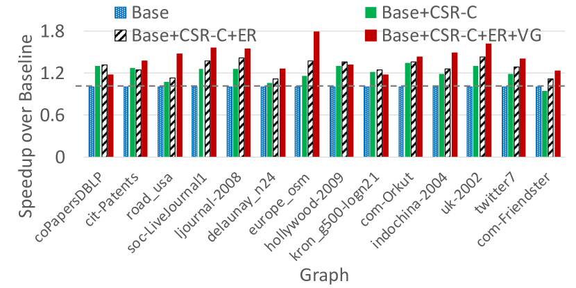
This section describes three key GPU optimizations—CSR coalescing (CSR-C), edge reorganization (ER), and vertex gathering (VG)—that we apply to our implementations in $\mathsf{GConn}$ . For practical purposes, we only consider the optimization strategies that improve the performance of the fastest $\mathsf{GConn}$ implementations. Since we found $\mathsf{Afforest}$ (Sutton et al., 2018) to be the fastest existing implementation in most cases, we identify the performance bottlenecks in $\mathsf{Afforest}$ , and show how to iteratively apply our optimizations to achieve the performance of our fastest implementations. We first substituted their union-find implementation with $\mathsf{Union\mathchar 45\relax Async}$ , which we found to be faster, and use this as the baseline. Figure 2 shows how performance improves over the baseline (Base) with each additional optimization applied.

CSR Coalescing (CSR-C). We identified that the sampling phase requires a significant amount of time in $\mathsf{Afforest}$ (35.15–98.63%, with a median of 88.80%), as shown in our experimental evaluation in Section 4.2. During $k$ -out sampling with $k=2$ , $\mathsf{Afforest}$ has two sub-phases, the first which traverses the first edge out of every vertex, and the second which traverses the second edge out of every vertex. This strategy traverses the scattered entries in the CSR array twice, which wastes memory bandwidth. Since the first two edges of a vertex are contiguous in the memory layout, the two edges of a vertex can be processed simultaneously by two adjacent threads, which makes memory accesses for the CSR array coalesced and halves the data volume needed to access the CSR array. We observe that applying this optimization on top of the baseline (Base+CSR-C in Figure 2) improves performance by an average of 20.68%.

Edge Reorganization (ER). During $k$ -out sampling, we found that CAS operations make the warp-efficiency on the GPU very low due to only a few threads in a warp being active. For these algorithms, if two edges having the same endpoint try to update a memory location at the same time, then the updates can become serialized. This is often the case in CSR format since edges incident to a single vertex are processed in the same warp. To alleviate this issue, we could have each thread read the first two edges of a vertex and process them sequentially; however, this would cause threads to have scattered accesses to the CSR edge array, which decreases memory efficiency. The edge reorganization optimization groups threads into pairs, where each pair reads the two edges for one vertex together, and then reads the two edges for another vertex together. Each time, the pair of threads reads contiguous locations in memory. Then, using warp shuffling (Catanzaro et al., 2014; Sung et al., 2014) the four edges can be reorganized so that the edges from the same vertex are contiguous in memory, enabling each thread to process the two edges of a vertex serially to avoid CAS operations. Base+CSR-C+ER in Figure 2 shows the performance improvement after applying ER on top of CSR-C. We achieve an average performance improvement of 28.79% over the baseline.

Vertex Gathering (VG). The previous optimizations improve the performance of the sampling phase. However, we found that the performance of the finish phase can also be improved. In the kernel for the finish phase in $\mathsf{Afforest}$ , each thread accesses entries in the $\mathit{labels}$ array in a cyclic fashion, and if the entry of the $i$ ’th label is not equal to $L_{\max}$ , then the edges of vertex $i$ are processed in a load-balanced fashion by distributing the edges across threads. However, as we show in Section 4.2, only a small subset of vertices have labels not equal to $L_{\max}$ . Therefore, many threads will be idle during the finish phase, which degrades performance. To improve performance in the finish phase, we first aggregate the vertices whose labels are not equal to $L_{\max}$ into an active vertex set, and in the finish phase, each thread reads a vertex in the active vertex set, and distributes the edges for load-balancing. We show the performance improvement of adding the vertex gathering optimization in Base+CSR-C+ER+VG of Figure 2. With all three optimizations, the overall performance is 41.55% faster than the baseline on average.

3.6. Incremental Connectivity Support

Algorithm 3

\mathsf{GConn}

for Incremental Connectivity

1:procedure Incremental(

G(V,E),\mathit{sample},\mathit{finish},\mathit{compress}

)

\mathit{labels}\leftarrow\textsc{StaticConn}(G(V,E),\mathit{sample},\mathit{finish},\mathit{compress})

3: for

B\in\mathit{Batches}

\mathit{(labels,query\_results)}\leftarrow

\textsc{FinishPhaseBatch}(B,\mathit{labels},\mathit{finish},\mathit{comp})

This section describes how $\mathsf{GConn}$ supports incremental connectivity given batches of updates. We support incremental connectivity for the root-based algorithms, and the pseudocode is shown in Algorithm 3. We first generate the initial graph (which can be empty) by initializing the $\mathit{labels}$ array for the vertices in the graph (Line 2) using the StaticConn procedure from Algorithm 1. We assume that the $\mathit{labels}$ array is large enough to hold all of the vertices that will be encountered, but we only initialize the entries for vertices present in the initial graph. Batches of insertions and connectivity queries arrive in an online fashion, and are processed using one of the finish algorithms on just the batch (Lines 3–4). The batches are given in COO format, which is a natural input for streaming algorithms. However, sampling is inefficient for graphs in COO format, and hence we do not use sampling for incremental algorithms.

Each batch $B$ is composed of a mix of inserts and queries. For an update, FinishPhaseBatch updates the $\mathit{labels}$ array as FinishPhase from Algorithm 1 does. Furthermore, a thread that inserts a new vertex will initialize its entry in the $\mathit{labels}$ array by acquiring a spin lock. For a query, FinishPhaseBatch calls the Find function (one of the compression algorithms $\mathsf{GConn}$ provides) for both query endpoints to check whether they are in the same component. The query results ( $\mathit{query\_results}$ in Line 4) are stored in a bitvector: the $i$ ’th entry in the bitvector is true if the $i$ ’th edge of $B$ is a query, and the two endpoints of it are in the same component.

As shown in Algorithm 3, the previous batches are never inspected because the root-based algorithms guarantee correctness without requiring inspecting edges in a previous batch (Dhulipala et al., 2020b). The root-based algorithms incorporated into $\mathsf{GConn}$ are all union-find algorithms used for static connectivity, $\mathsf{Shiloach\mathchar 45\relax Vishkin}$ , and the root-based $\mathsf{Liu\mathchar 45\relax Tarjan}$ algorithms. However, when $\mathsf{Union\mathchar 45\relax}$ $\mathsf{Rem\mathchar 45\relax CAS}$ and $\mathsf{Union\mathchar 45\relax Rem\mathchar 45\relax Lock}$ with $\mathsf{SpliceAtomic}$ is used, the updates and queries need to be processed separately to guarantee correctness (Dhulipala et al., 2020b).

4. Evaluation

In this section, we provide an experimental evaluation and analysis of $\mathsf{GConn}$ . All numbers reported in this section are the median of five runs on the Volta machine unless noted otherwise. We found that the trends for spanning forest are similar to the trends for connectivity, with our spanning forest implementations obtaining an average speedup of 6% over the connectivity implementations due to not requiring the label finalization step.

Overview of Results. The results of this section can be summarized as follows:

•

We provide an experimental evaluation of $\mathsf{GConn}$ connectivity implementations in the no sampling setting (Section 4.1). Without sampling, $\mathsf{Union\mathchar 45\relax Async}$ and $\mathsf{Union\mathchar 45\relax Rem\mathchar 45\relax CAS}$ are the fastest implementations.
•

In the sampling setting, we provide a detailed analysis of different sampling procedures and find that $k$ -out sampling or HB sampling can significantly improve the performance unless the average degree of vertices is low (Section 4.2).
•

The fastest $\mathsf{GConn}$ algorithms consistently and significantly outperform state-of-the-art GPU connectivity implementations (Section 4.3).
•

$\mathsf{GConn}$ incremental connectivity algorithms can achieve a throughput of tens of billions of edges per second. We also evaluate the throughput for different batch sizes, and ratios of insertions to queries (Section 4.4). In the incremental setting, $\mathsf{Union\mathchar 45\relax Async}$ is usually the fastest implementation.
•

Compared to $\mathsf{ConnectIt}$ , a framework for CPU connectivity algorithms, $\mathsf{GConn}$ achieves 8.26–14.51x speedup for static connectivity and 1.85–13.36x speedup for incremental connectivity. Our analyses also show GPUs are an attractive platform for connectivity algorithms in terms of both speed and cost (Section 4.6).

Dataset	$n$	$m$	Diam.	Num. Comps.	Largest Comp.
coPapersDBLP	540.49K	30.49M	15*	1	540.49K
cit-Patents	3.77M	33.04M	20*	3,627	3.76M
road_usa	23.95M	57.71M	6,809	1	23.95M
soc-LiveJournal1	4.85M	85.70M	16	1,876	4.84M
ljournal-2008	5.36M	99.03M	31*	75	5.36M
delaunay_n24	16.78M	100.66M	1,720*	1	16.78M
europe_osm	50.91M	108.11M	19,314*	1	50.91M
hollywood-2009	1.14M	112.75M	11	44,508	1.07M
kron_g500-logn21	2.10M	182.08M	6	553,159	1.54M
com-Orkut	3.07M	234.37M	9	1	3.07M
indochina-2004	7.41M	301.97M	26	295	7.32M
uk-2002	18.52M	523.57M	29*	38,359	18.46M
twitter7	41.65M	2.41B	23*	1	41.65M
com-Friendster	65.61M	3.61B	32	1	65.61M

Table 1. Graph inputs, including number of vertices (

n

), edges (

m

), diameter, number of connected components, and the largest connected component. The graphs are symmetric, and edges are counted once in each direction. For graphs on which we were unable to compute the exact diameter, we compute the effective diameter (marked with *), which is a lower bound on the actual diameter.

Experimental Setup. Our GPU evaluation is performed on two machines. The first is an NVIDIA Tesla V100, which is a Volta generation GPU with 32GB that offers a 900 GB/sec memory bandwidth, 6MB of L2 cache, and 128KB of L1 cache per Streaming Multiprocessor (SM) with a total of 80 SMs. The second is an NVIDIA TITAN Xp, which is a Pascal generation GPU with 12GB that offers a 547.6 GB/sec memory bandwidth, 3MB of L2 cache, and 48KB of L1 cache per SM with a total of 30 SMs. All implementations are compiled with NVCC v10.0 using the -O3 and --use_fast_math flags.

Graph Data. To show how $\mathsf{GConn}$ performs on various graphs of different scales, we selected all publicly-available graphs used in $\mathsf{ECL\mathchar 45\relax CC}$ (Jaiganesh and Burtscher, 2018), $\mathsf{EvoGraph}$ (Sengupta and Song, 2017), and $\mathsf{ConnectIt}$ (Dhulipala et al., 2020b) that have more than 30M edges and fit in the GPU memory. Table 1 shows the details of our graph inputs, including the number of vertices and edges, the graph diameter, the number of connected components, and the size of the largest component. Our inputs include many Web and social network graphs that have low diameters, as well as road networks that have high diameters. All graphs that we use were obtained from SuiteSparse (Davis and Hu, 2011) or SNAP (Leskovec and Krevl, 2019). We symmetrized all of the graphs.

Group

Algorithm

coPapers

DBLP

cit-

Patents

road_usa

soc-Live

Journal1

ljournal

-2008

delaunay

_n24

europe

_osm

hollywood

-2009

kron_g500

-logn21

com-

Orkut

indochina

-2004

uk-2002

twitter7

com-

Friendster

No sampling

\mathsf{Union\mathchar 45\relax Early}

1.49

4.79

5.68

8.18

8.83

17.65

6.87

8.14

16.23

14.11

26.39

32.89

375.50

853.87

\mathsf{Union\mathchar 45\relax Hooks}

0.68

3.44

5.56

3.94

5.26

5.98

11.67

1.95

4.65

4.02

7.36

13.97

155.98

410.61

\mathsf{Union\mathchar 45\relax Async}

0.46

2.02

3.39

3.07

3.17

3.84

6.76

1.62

3.64

3.85

5.32

9.09

123.78

365.98

\mathsf{Union\mathchar 45\relax Rem\mathchar 45\relax CAS}

0.45

1.88

3.83

2.98

3.20

4.09

5.90

1.53

3.60

3.70

5.39

9.26

133.46

369.59

\mathsf{Union\mathchar 45\relax Rem\mathchar 45\relax Lock}

0.90

4.66

9.57

5.73

7.59

10.31

11.45

2.73

6.52

4.19

65.96

93.69

484.23

487.72

\mathsf{Union\mathchar 45\relax JTB}

0.53

2.84

5.53

3.70

3.68

5.29

10.85

1.96

5.23

5.78

6.40

11.07

130.01

400.17

\mathsf{Liu\mathchar 45\relax Tarjan}

1.20

6.73

12.13

7.72

11.27

12.60

31.23

4.69

12.39

10.16

21.53

31.44

464.76

998.77

\mathsf{Shiloach\mathchar 45\relax Vishkin}

1.47

13.05

15.65

12.23

17.17

18.63

34.49

7.57

15.93

34.09

35.01

47.73

1056.17

2066.00

\mathsf{LabelPropagation}

2.57

8.98

3289.59

15.01

58.89

1032.09

2.14e4

6.18

12.50

18.58

79.25

112.74

1361.37

3646.96

\mathsf{G\_ECL\mathchar 45\relax CC}

0.51

2.26

3.76

3.18

3.80

4.19

10.09

1.92

3.84

5.01

6.75

11.58

161.13

385.48

\mathsf{G\_Afforest}

5.96

23.07

4.01

25.46

42.12

6.70

19.07

85.02

91.66

97.24

43.12

73.80

143.75

1661.75

k

-out sampling

\mathsf{Union\mathchar 45\relax Early}

0.26

3.30

8.93

1.28

1.85

6.34

9.50

0.74

0.85

1.00

7.33

7.83

22.59

49.34

\mathsf{Union\mathchar 45\relax Hooks}

0.20

2.52

8.13

1.05

1.63

4.87

10.57

0.39

0.61

0.74

2.42

4.39

14.01

31.09

\mathsf{Union\mathchar 45\relax Async}

0.18

1.60

5.27

0.85

1.19

3.60

6.95

0.35

0.51

0.63

2.07

3.46

10.91

27.79

\mathsf{Union\mathchar 45\relax Rem\mathchar 45\relax CAS}

0.16

1.98

5.98

0.86

1.38

3.44

7.78

0.33

0.53

0.62

1.86

3.52

12.81

44.87

\mathsf{Union\mathchar 45\relax Rem\mathchar 45\relax Lock}

0.71

3.79

13.28

1.80

3.00

8.46

13.57

0.98

0.99

0.74

35.74

41.10

26.83

53.61

\mathsf{Union\mathchar 45\relax JTB}

0.24

2.31

6.97

1.27

1.75

4.66

13.38

0.47

0.65

0.86

2.95

5.04

13.80

32.20

\mathsf{Liu\mathchar 45\relax Tarjan}

1.29

11.56

20.71

3.07

13.96

15.19

40.17

5.20

13.05

0.65

20.20

26.76

41.69

522.27

\mathsf{Shiloach\mathchar 45\relax Vishkin}

1.55

18.88

21.35

12.68

17.37

17.42

47.61

8.46

15.99

33.79

32.47

67.94

1150.68

2059.18

\mathsf{LabelPropagation}

2.28

16.44

8228.75

2.67

72.57

895.65

65136.83

8.32

18.65

0.60

103.27

134.05

27.01

163.80

\mathsf{G\_ECL\mathchar 45\relax CC}

0.19

1.67

4.88

0.88

1.28

3.19

7.28

0.38

0.56

0.66

2.11

3.80

11.14

27.29

\mathsf{G\_Afforest}

0.24

4.72

5.63

1.25

4.40

3.81

9.58

0.84

2.41

0.80

2.79

5.60

13.46

31.84

HB sampling

\mathsf{Union\mathchar 45\relax Early}

0.41

2.59

17.79

1.03

1.86

48.33

25.42

1.48

0.76

0.49

12.95

17.26

12.62

19.26

\mathsf{Union\mathchar 45\relax Hooks}

0.24

1.75

12.45

0.70

1.41

7.37

16.78

0.43

0.64

0.50

3.00

5.99

9.90

17.97

\mathsf{Union\mathchar 45\relax Async}

0.24

1.47

8.60

0.67

1.22

5.95

14.99

0.41

0.57

0.49

2.60

4.97

9.12

17.75

\mathsf{Union\mathchar 45\relax Rem\mathchar 45\relax CAS}

0.24

1.56

8.62

0.67

1.28

6.37

13.66

0.41

0.57

0.50

2.43

4.83

9.60

18.30

\mathsf{Union\mathchar 45\relax Rem\mathchar 45\relax Lock}

1.51

2.39

14.37

8.16

1.90

9.63

17.11

0.60

1.59

0.49

10.60

20.95

11.78

19.09

\mathsf{Union\mathchar 45\relax JTB}

0.70

5.68

8.54

6.09

5.37

7.09

18.86

2.56

11.11

15.28

9.78

12.13

339.15

738.97

\mathsf{Liu\mathchar 45\relax Tarjan}

1.36

11.68

21.85

1.91

10.53

24.67

40.01

3.70

9.06

0.61

15.80

27.15

14.33

353.80

\mathsf{Shiloach\mathchar 45\relax Vishkin}

2.94

18.55

21.38

6.33

14.49

24.37

54.87

9.20

27.01

0.64

25.44

67.48

46.30

829.49

\mathsf{LabelPropagation}

6.58

16.62

7943.94

2.22

73.01

982.00

6.65e04

8.24

19.12

0.57

97.24

125.14

24.71

123.77

\mathsf{G\_ECL\mathchar 45\relax CC}

0.26

1.39

8.44

0.71

1.23

6.32

14.21

0.47

0.61

0.50

2.71

5.28

8.78

17.57

\mathsf{G\_Afforest}

0.26

2.85

8.04

0.73

2.03

9.12

13.80

0.55

1.14

0.50

3.56

6.22

10.83

17.75

BFS sampling

\mathsf{Union\mathchar 45\relax Early}

1.34

2.39

409.15

2.10

2.67

90.27

1778.75

1.25

0.81

1.06

80.15

35.55

22.20

20.58

\mathsf{Union\mathchar 45\relax Hooks}

1.35

2.38

391.73

1.90

2.68

92.41

1652.54

1.22

0.80

1.03

79.23

32.24

22.19

20.56

\mathsf{Union\mathchar 45\relax Async}

1.32

2.40

390.92

1.93

2.68

92.91

1578.57

1.23

0.83

1.05

80.58

32.54

22.22

20.54

\mathsf{Union\mathchar 45\relax Rem\mathchar 45\relax CAS}

1.34

2.38

397.09

2.07

2.78

90.25

1598.75

1.26

0.82

1.03

79.64

32.32

22.16

20.52

\mathsf{Union\mathchar 45\relax Rem\mathchar 45\relax Lock}

1.32

2.38

399.62

2.06

2.74

92.41

1584.45

1.26

0.80

1.02

83.84

33.09

22.19

20.52

\mathsf{Union\mathchar 45\relax JTB}

1.36

2.53

406.20

2.21

3.06

104.46

1627.93

1.29

0.89

1.18

80.51

32.89

23.98

23.72

\mathsf{Liu\mathchar 45\relax Tarjan}

1.38

3.14

395.90

2.55

2.92

91.79

1659.59

1.44

1.04

1.10

81.54

35.14

22.57

21.19

\mathsf{Shiloach\mathchar 45\relax Vishkin}

1.41

3.07

401.61

2.50

2.90

97.07

1616.75

1.53

1.05

1.15

82.49

34.78

23.29

22.19

\mathsf{LabelPropagation}

1.39

3.23

403.12

2.49

2.77

93.34

1626.54

1.51

0.95

1.07

89.03

40.99

22.35

20.86

\mathsf{G\_ECL\mathchar 45\relax CC}

1.33

2.41

397.33

2.06

2.82

94.21

1631.24

1.24

0.83

1.06

81.36

32.57

22.20

20.51

\mathsf{G\_Afforest}

1.30

2.39

393.34

2.06

2.80

91.45

1625.83

1.30

0.83

1.06

83.19

32.84

22.18

20.48

Existing algorithms

\mathsf{GPU\mathchar 45\relax CC}

(Soman et al., 2010)

2.77

9.74

22.85

10.18

31.5

22.83

46.38

21.38

34.04

21.25

44.96

49.01

417.25

\mathsf{x}

\mathsf{GSWITCH}

(Meng et al., 2019)

1.07

4.5

21.03

7.06

9.24

8.22

38.39

6.82

7.45

7.54

13.46

26.1

\mathsf{x}

\mathsf{x}

\mathsf{ECL\mathchar 45\relax CC}

(Jaiganesh and Burtscher, 2018)

0.78

5.89

22.55

7.14

7.71

18.94

25.97

2.1

6.02

8.58

9.06

26.31

258.56

415.44

\mathsf{Afforest}

(Sutton et al., 2018)

0.35

6.13

5.54

1.27

5.07

3.69

9.13

1.06

2.97

0.82

4.55

7.67

13.5

32.4

\mathsf{BFS\mathchar 45\relax CC}

1.33

721.59

577.38

277.35

8.51

89.33

1749.63

4267.22

5.07e04

0.96

133.77

3698.56

21.07

19.22

Table 2. Running times of implementations in

\mathsf{GConn}

and state-of-the-art static connectivity algorithms in miliseconds on a V100 GPU. We report running times for five groups: implementations with No sampling,

k

-out sampling, HB sampling, BFS sampling, and existing algorithms. Within each of the first four group, we display the fastest variant for each graph in green. For each graph, we also display the fastest variant across all groups in bold font.

\mathsf{x}

means that we were unable to obtain results due to the graph not fitting in the GPU memory for the given implementation.

4.1. Static Parallel Connectivity without Sampling

In this section, we evaluate our $\mathsf{GConn}$ implementations for static connectivity algorithms in the No Sampling setting.

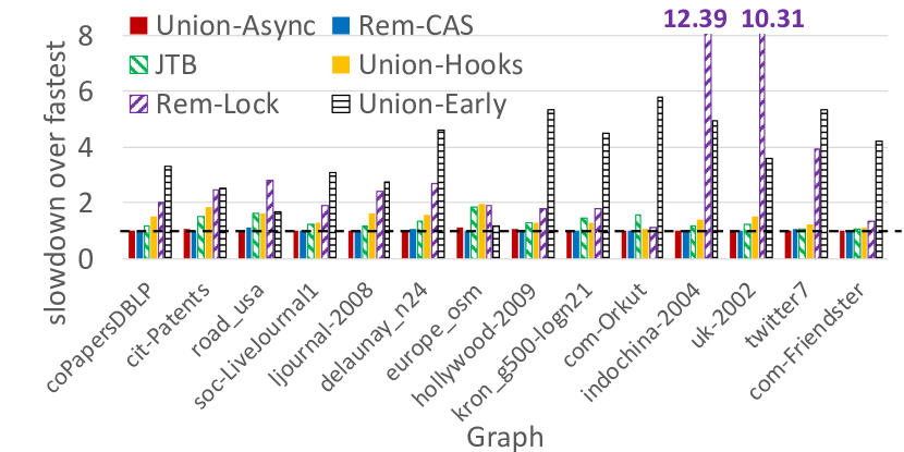
Evaluation of Union-Find Variants. The first group of rows in Table 2 shows the results of the fastest implementations of each algorithm in the no sampling setting.

Figure 3 shows the slowdown of the fastest of each of the union-find variants over the fastest overall variant for each graph. For each graph, six bars are listed in order of average performance. From Figure 3, we observe that the fastest implementation is either $\mathsf{Union\mathchar 45\relax Async}$ or $\mathsf{Union\mathchar 45\relax Rem\mathchar 45\relax CAS}$ in the No Sampling setting. $\mathsf{Union\mathchar 45\relax Rem\mathchar 45\relax CAS}$ is 1.02x slower on average than $\mathsf{Union\mathchar 45\relax Async}$ across all graphs, and $\mathsf{Union\mathchar 45\relax JTB}$ is 1.26x slower on average than $\mathsf{Union\mathchar 45\relax Async}$ due to the usage of 64-bit CAS operations. $\mathsf{Union\mathchar 45\relax}$ $\mathsf{Hooks}$ is designed to reduce the overhead for atomic operations, but it is 1.44x slower on average than $\mathsf{Union\mathchar 45\relax Async}$ due to a costly memory barrier needed to avoid race conditions. $\mathsf{Union\mathchar 45\relax Rem\mathchar 45\relax Lock}$ is 3.81x slower on average than $\mathsf{Union\mathchar 45\relax Rem\mathchar 45\relax CAS}$ due to the poor performance of spin locks on GPUs.

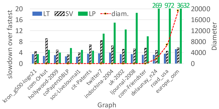
Evaluation of Other Min-based Algorithms. Figure 4 shows the slowdown of the other min-based algorithms compared to the fastest variant across all algorithms in the no-sampling setting. The graphs that are sorted in order of increasing diameter (presented with the red curve).

As shown in Figure 4, the other min-based algorithms are much slower than the union-find algorithms because union-find algorithms only inspect each edge at once, whereas the other algorithms typically traverse edges multiple times, which leads to redundant computation. The fastest $\mathsf{Liu\mathchar 45\relax Tarjan}$ and $\mathsf{Shiloach\mathchar 45\relax Vishkin}$ variants are 3.72x and 5.19x slower on average than $\mathsf{Union\mathchar 45\relax Async}$ in the no-sampling setting, respectively. We have included the $\mathsf{Stergiou}$ algorithm in the category of $\mathsf{Liu\mathchar 45\relax Tarjan}$ algorithms as this algorithm is similar to $\mathsf{Liu\mathchar 45\relax Tarjan}$ algorithms; however, it is always much slower than the fastest variant of $\mathsf{Liu\mathchar 45\relax Tarjan}$ algorithms (up to 66x slower).

As shown for the three graphs located on the far right in Figure 4, the performance of $\mathsf{LabelPropagation}$ degrades significantly as the diameter increases. This is because $\mathsf{LabelPropagation}$ needs a large number of rounds to propagate the minimum label to all vertices, and during that time most vertices are active. Even on low-diameter graphs (diameter at most 32 in our experiments), $\mathsf{LabelPropagation}$ is still 7.76x slower on average than the union-find algorithms since $\mathsf{LabelPropagation}$ still requires multiple traversals per edge, whereas the union-find algorithms do not.

As shown in Table 2, we also incorporate the finish algorithms used in two fastest state-of-the-art works, $\mathsf{ECL\mathchar 45\relax CC}$ (Jaiganesh and Burtscher, 2018) (denoted as $\mathsf{G\_ECL\mathchar 45\relax CC}$ ) and $\mathsf{Afforest}$ (Sutton et al., 2018) (denoted as $\mathsf{G\_Afforest}$ ), into $\mathsf{GConn}$ , and evaluate them in Section 4.3.

4.2. Static Parallel Connectivity with Sampling

This section studies how our three sampling strategies affect performance, in terms of their execution time and the quality of the resulting sub-problem that they generate for the finish step in $\mathsf{GConn}$ . We start by studying how $k$ -out sampling performs.

Evaluation of $k$ -out sampling. The second group of rows in Table 2 presents the results of the fastest implementations of each algorithm using $k$ -out sampling. The fastest implementation is $\mathsf{Union\mathchar 45\relax Async}$ , $\mathsf{Union\mathchar 45\relax Rem\mathchar 45\relax CAS}$ , or $\mathsf{G\_ECL\mathchar 45\relax CC}$ ; $\mathsf{Union\mathchar 45\relax Rem\mathchar 45\relax CAS}$ is 1.03x slower on average than $\mathsf{Union\mathchar 45\relax Async}$ , and we defer the analysis for $\mathsf{G\_ECL\mathchar 45\relax CC}$ to Section 4.3.

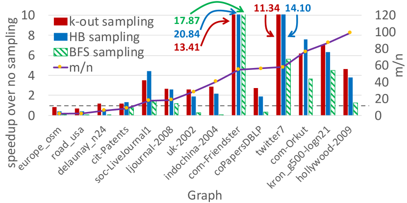
Figure 5 shows how each sampling algorithm improves performance. To see the performance improvement with respect to the average degree of the vertices (i.e., $m/n$ ), we sorted the graphs in ascending order of the average degree.

For the union-find variants, except on the two road-network graphs (road_usa and europe_osm), $k$ -out sampling improves performance over the unsampled versions by 6.16x on average due to the significant reduction of edges that need to be inspected, as we will show shortly. For the other min-based algorithms, other than on the two road-network graphs, $k$ -out sampling improves performance by 4.61x on average over the unsampled versions.

As shown in Figure 5, when the average degree is small (e.g., road_usa and europe_osm), $k$ -out sampling as well as other sampling algorithms degrades performance. This is because most of the edges in the graph get inspected in the sampling phase, and there is additional overhead to split the computation across two phases. In general, $k$ -out sampling decreases the number of edge inspections by up to $m-kn$ , and so as the average degree increases, we can expect a higher potential performance improvement. As shown in Figure 5, $k$ -out sampling usually shows better performance when the average degree is large.

Evaluation of HB sampling. The third group of rows in Table 2 presents the fastest variants of each algorithm using HB sampling with a default value of $N=4$ , which we found to work the best on average across our input graphs.¹¹1 Although the optimal value of $N$ can vary based on the input graph, determining the optimal value on a per-graph basis would incur significant overhead, which would outweigh the benefits of using the optimal parameter as opposed to the default parameter. Unlike $k$ -out sampling, HB sampling does not always improve performance; in many cases, the performance is degraded. The overall trend of HB sampling is similar to that of $k$ -out sampling. As shown in Figure 5, when the average degree of vertices is small, HB sampling significantly degrades performance, and otherwise HB sampling can greatly improve performance. We will discuss how HB sampling compares with our other sampling schemes shortly.

Evaluation of BFS sampling. The fastest variants using BFS sampling are presented in the fourth group in Table 2. The effectiveness of BFS sampling is dependent on the diameter of an input graph and the parameters for the direction-optimizing BFS. As shown in Figure 5, for the high-diameter graphs (the three graphs on the far left), BFS sampling degrades performance by 24.59x on average over the unsampled versions due to the very small active vertex set for each BFS iteration and since a GPU kernel must be launched for each iteration. For the other graphs, BFS sampling achieves a 0.07–174.87x speedup over the unsampled versions. Note that as shown in the last row of Table 2, we also implemented the $\mathsf{BFS\mathchar 45\relax CC}$ algorithm introduced in $\mathsf{Ligra}$ (Shun and Blelloch, 2013), in which a BFS is repeated on each new component until all components are found. $\mathsf{BFS\mathchar 45\relax CC}$ performs poorly due to the GPU kernel launch overhead for high-diameter graphs and for graphs with many connected components.

Graph

BFS

Time

BFS

Cov

BFS

KOut

Time

KOut

Cov

KOut

Time

Cov

coPapersDBLP

60.3%

100.0%

0.0%

46.7%

98.9%

0.2%

97.2%

89.1%

5.4%

cit-Patents

83.9%

99.7%

0.0%

90.1%

98.2%

0.6%

99.5%

96.0%

2.3%

road_usa

86.8%

100.0%

0.0%

85.4%

95.9%

3.6%

83.1%

0.0%

100.0%

soc-LiveJournal1

86.9%

99.9%

0.0%

91.0%

99.9%

0.0%

92.1%

99.5%

1.1%

ljournal-2008

92.1%

100.0%

0.0%

83.7%

99.3%

0.2%

92.0%

94.9%

2.5%

delaunay_n24

92.3%

100.0%

0.0%

76.9%

100.0%

0.0%

89.3%

0.0%

100.0%

europe_osm

92.4%

100.0%

0.0%

79.2%

100.0%

0.0%

92.4%

0.0%

100.0%

hollywood-2009

55.1%

93.8%

0.1%

42.0%

91.0%

0.5%

99.8%

87.4%

2.0%

kron_g500-logn21

93.5%

73.6%

0.0%

41.2%

73.6%

0.0%

99.7%

73.5%

0.0%

com-Orkut

74.4%

100.0%

0.0%

54.4%

100.0%

0.0%

97.8%

100.0%

0.0%

indochina-2004

90.3%

98.7%

1.3%

42.5%

86.8%

7.4%

99.5%

63.2%

24.4%

uk-2002

95.9%

99.7%

0.1%

90.2%

92.0%

4.9%

88.2%

72.4%

20.8%

twitter7

93.4%

100.0%

0.0%

39.4%

100.0%

0.0%

99.7%

99.5%

0.0%

com-Friendster

98.0%

100.0%

0.0%

95.2%

100.0%

0.0%

90.3%

99.9%

0.0%

Table 3. This table presents how effective the sampling strategy is for each of our graph inputs. The Time columns show the percentage of sampling time to the total execution time. The Cov columns show the percentage of vertices that are in the largest connected component after the sampling phase. Hence, the edges incident to these vertices are not inspected in the finish phase. The IC columns show the percentage of inter-component edges that will be processed in the finish phase.

Comparing Different Sampling Strategies. Table 3 shows how many vertices and edges are covered by each sampling algorithm. As shown in Table 3, since BFS traverses all vertices connected to a source vertex likely to be in the largest connected component, the fraction of vertices covered (Cov) and the fraction of remaining inter-component edges (IC) are maximized and minimized, respectively. Unfortunately, as shown in Table 2, BFS sampling takes significantly longer than other sampling algorithms, especially for the high-diameter graphs (delaunay_n24, road_usa, and europe_osm) due to the kernel launch overhead and low parallelism on these graphs. It also inspects significantly more edges than the other two schemes, as we will show shortly. Although BFS sampling usually takes longer than $k$ -out sampling, we observe that Cov and IC for BFS sampling and $k$ -out sampling are very similar on our inputs. The sampling time for HB sampling is much lower than for the others due to the reduced number of edge inspections, but for some graphs, CoV and IC are significantly lower than for the other two schemes (especially for high-diameter graphs). The Time columns in Table 3 show the ratio of the sampling time to the total execution time. We see that the sampling phase takes most of the time, and hence, the design of an efficient, high-quality sampling algorithm is of paramount importance.

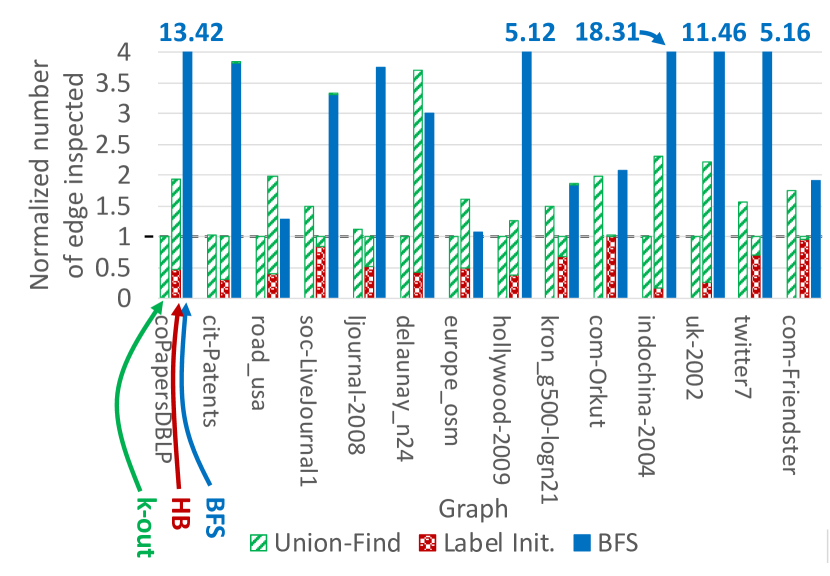
Figure 6 shows the normalized total number of edges inspected during the execution of each sampling algorithm. For each graph, Figure 6 shows three bars. The first bar (green only) corresponds to the number of edges inspected by $k$ -out sampling using union-find. The second bar (red and green) shows the number of edges inspected during the label initialization step, and the union-find step of HB sampling, respectively. Finally, the third bar (blue) shows the number of edges inspected by BFS sampling. From Table 2 and Figure 6, we observe that BFS sampling is never the fastest, and HB sampling is the fastest when the number of edge inspections for union-find is small during the sampling phase. In this case, the total number of edge inspections is also minimized. For com-Friendster, as shown in Table 2, BFS sampling is faster than $k$ -out sampling; the number of edge inspections with BFS sampling is usually the highest, but for com-Friendster, the total number of edge inspections for both BFS sampling and $k$ -out sampling is similar, and thus BFS sampling is faster because the edge inspection step performed by the BFS (a single CAS on one of the endpoints) is much faster than the edge inspection by a union-find algorithm (a loop that must potentially run multiple times due to contention). As seen in Figures 5 and 6, for some graphs (e.g., indochina-2004, which has a speedup of 0.07x), the number of edge inspections is much higher for BFS, leading to significant performance degradation.

4.3. Comparison with State-of-the-art

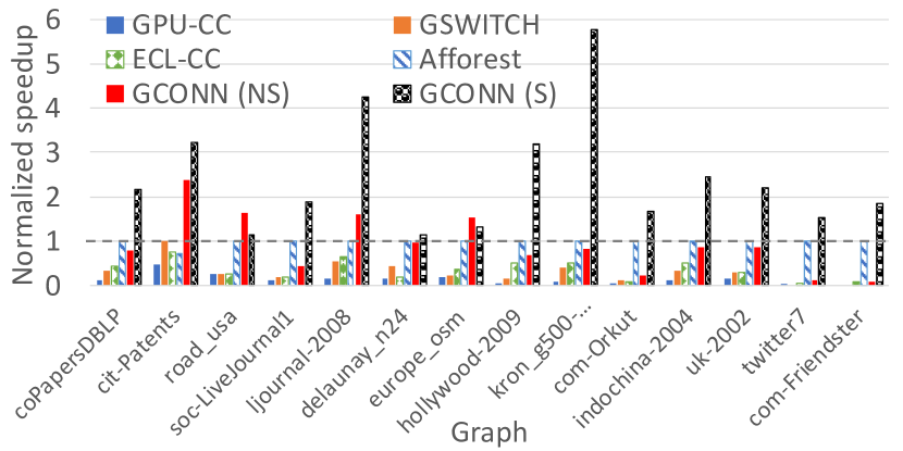
This section compares our implementations with current state-of-the-art connectivity implementations on GPUs, which are shown in the last group of rows in Table 2. Figure 7 presents the normalized execution time over the fastest current state-of-the-art implementation for each graph with our fastest variant without and with sampling. Note that we did not report results for $\mathsf{Groute}$ (Ben-Nun et al., 2017), $\mathsf{Gunrock}$ (Wang et al., 2016), and $\mathsf{IrGL}$ (Pai and Pingali, 2016) as they are outperformed by $\mathsf{ECL\mathchar 45\relax CC}$ (Jaiganesh and Burtscher, 2018), which we compare against. We also tried the strategy by Cong and Muzio (Cong and Muzio, 2014), but it never gave the best performance.

$\mathsf{GPU\mathchar 45\relax CC}$ (Soman et al., 2010) and $\mathsf{GSWITCH}$ (Meng et al., 2019). $\mathsf{GPU\mathchar 45\relax CC}$ adopts a classic SV algorithm, which turns out to be slow as shown in Figure 7. Our fastest implementations without sampling and with sampling are 7.06x and 26.68x faster on average than $\mathsf{GPU\mathchar 45\relax CC}$ , respectively. $\mathsf{GSWITCH}$ also applies a classic SV algorithm, but outperforms $\mathsf{GPU\mathchar 45\relax CC}$ due to several additional optimizations. Our fastest implementations without sampling and with sampling are 3.24x and 8.88x faster on average than $\mathsf{GSWITCH}$ .

$\mathsf{ECL\mathchar 45\relax CC}$ (Jaiganesh and Burtscher, 2018). $\mathsf{ECL\mathchar 45\relax CC}$ is faster than both $\mathsf{GPU\mathchar 45\relax CC}$ and $\mathsf{GSWITCH}$ due to using a more efficient algorithm based on union-find. As shown in Figure 7, our fastest implementations without sampling and with sampling are 2.78x and 10.15x faster on average than $\mathsf{ECL\mathchar 45\relax CC}$ , respectively, mainly because we use a more efficient load-balancing strategy, and more efficient find and compress rules.

We also implemented the finish algorithm $\mathsf{G\_ECL\mathchar 45\relax CC}$ that is used in $\mathsf{ECL\mathchar 45\relax CC}$ . As shown in Table 2, $\mathsf{G\_ECL\mathchar 45\relax CC}$ without sampling is 2.30x faster on average than $\mathsf{ECL\mathchar 45\relax CC}$ . The speedup comes from using a different load-balancing strategy; in $\mathsf{ECL\mathchar 45\relax CC}$ , one thread handles all edges of a vertex with degree at most 16, which can lead to significant load-imbalance. In contrast, $\mathsf{GConn}$ enables those edges to be processed in a load-balanced fashion using a variation of a strategy by Merrill et al. (Merrill et al., 2012) that we designed. Without sampling and with sampling, $\mathsf{G\_ECL\mathchar 45\relax CC}$ is 1.19x and 1.04x slower on average than our fastest variants, respectively.

$\mathsf{Afforest}$ (Sutton et al., 2018). $\mathsf{Afforest}$ also implements a root-based algorithm with $k$ -out sampling. As shown in Figure 7, our fastest implementations without sampling are 1% slower on average than $\mathsf{Afforest}$ with sampling due to the fact that many edges are not inspected in $\mathsf{Afforest}$ . Our fastest implementations with sampling are 2.51x faster on average because variants using HB sampling sometimes outperform those using $k$ -out sampling, and the finish algorithm used in $\mathsf{Afforest}$ is slower than those used in our fastest variants. We also implemented $\mathsf{G\_Afforest}$ , the finish algorithm used in $\mathsf{Afforest}$ , in $\mathsf{GConn}$ . We found that compared to other finish algorithms in the no sampling setting, $\mathsf{G\_Afforest}$ is 12.6x slower on average than our fastest finish algorithm. The main reason seems to be due to some union-find algorithms, such as $\mathsf{Union\mathchar 45\relax Async}$ and $\mathsf{Union\mathchar 45\relax Rem\mathchar 45\relax CAS}$ , handling path compression more efficiently than the method used in $\mathsf{G\_Afforest}$ .

4.4. Incremental Parallel Graph Connectivity

In this section, we evaluate incremental connectivity algorithms on GPUs. We achieve a raw speedup of 2,482x over $\mathsf{EvoGraph}$ (Sengupta and Song, 2017) which is the fastest current state-of-the-art streaming connectivity implementation. Furthermore, the memory bandwidth-normalized speedup is 794x over $\mathsf{EvoGraph}$ . Unfortunately, we are not able to directly compare our streaming connectivity implementations with existing implementations on the same machine, although we provide indirect comparisons based on the numbers provided by the authors in their paper.²²2We contacted the authors for their code, but were unable to obtain it. $\mathsf{cuSTINGER}$ (Green and Bader, 2016) and $\mathsf{Hornet}$ (Busato et al., 2018) are GPU frameworks for streaming graphs, but their code does not contain streaming connectivity algorithms.

We conduct two types of streaming experiments. In the first type of experiment, we generate a stream of edge updates from the input graphs in Table 1. The second type of experiment models real-world graph streams using synthetic graph generators. Specifically, we use the RMAT generator (Chakrabarti et al., 2004) with parameters $(a,b,c)=(0.5,0.1,0.1)$ and the Barabasi-Albert (BA) generator (Barabasi and Bonabeau, 2003). For both generators, we use $n=2^{27}$ and $m=10n$ . The edges in a batch are given in COO format, and are unsorted.

Algorithm

coPapers

DBLP

cit-

Patents

road_usa

soc-Live

Journal1

ljournal

-2008

delaunay

_n24

europe

_osm

hollywood

-2009

kron_g500

-logn21

com-

Orkut

indochina

-2004

uk-2002

twitter7

com-

Friendster

RMAT

\mathsf{Union\mathchar 45\relax Early}

8.18e09

6.08e09

5.44e09

5.19e09

3.78e09

4.87e09

6.83e09

4.65e09

4.37e09

5.58e09

2.39e09

3.42e09

3.19e09

1.78e09

3.67e09

7.50e08

\mathsf{Union\mathchar 45\relax Hooks}

2.66e10

7.51e09

5.69e09

1.17e10

9.58e09

8.78e09

4.75e09

3.52e10

2.65e10

4.26e10

1.29e10

1.18e10

5.54e09

9.95e09

4.81e09

\mathsf{Union\mathchar 45\relax Async}

3.17e10

1.27e10

7.35e09

1.72e10

1.31e10

1.24e10

6.74e09

3.93e10

3.25e10

4.66e10

1.59e10

1.65e10

1.51e10

6.08e09

1.17e10

5.03e09

\mathsf{Union\mathchar 45\relax Rem\mathchar 45\relax CAS}

1.05e10

6.50e09

4.46e09

6.20e09

4.00e09

5.70e09

6.05e09

7.64e09

1.03e10

1.16e10

1.98e09

3.27e09

3.80e09

3.14e09

5.60e09

9.61e08

\mathsf{Union\mathchar 45\relax Rem\mathchar 45\relax Lock}

3.25e09

5.45e09

3.48e09

1.96e09

4.97e08

5.50e09

4.44e09

6.20e09

1.94e10

4.49e10

4.14e07

1.55e08

5.46e08

7.23e09

1.11e10

4.17e09

\mathsf{Union\mathchar 45\relax JTB}

2.78e10

8.70e09

5.29e09

1.33e10

9.39e09

8.63e09

4.68e09

3.32e10

2.52e10

2.94e10

1.14e10

1.21e10

1.41e10

5.85e09

8.14e09

5.70e09

\mathsf{Liu\mathchar 45\relax Tarjan}

1.39e10

2.50e09

2.92e09

7.41e09

6.99e09

4.62e09

2.63e09

1.42e10

7.38e09

1.18e10

8.85e09

9.56e09

4.74e09

2.08e09

3.05e09

2.28e09

\mathsf{Shiloach\mathchar 45\relax Vishkin}

9.42e09

2.09e09

2.97e09

5.39e09

4.27e09

3.12e09

2.02e09

4.84e09

3.90e09

3.79e09

5.90e09

7.90e09

3.22e09

1.37e09

2.50e09

2.36e09

Table 4. Throughput achieved by incremental connectivity algorithms in

\mathsf{GConn}

on a V100 GPU machine when all of the edges in the graph are treated as a single batch of updates. For each graph, the highest throughput is shown in green.

Throughput. We evaluate the throughput of our incremental connectivity implementations on all of the input graphs in Table 2, and the two large synthetic graphs generated from the RMAT and BA generators. Table 4 reports the streaming throughput achieved by the fastest variant of each algorithm for each input when all of the edges are treated as a single batch of updates.

As shown in Table 4, the $\mathsf{Union\mathchar 45\relax Async}$ algorithm usually achieves the highest throughput. Recall that for static parallel connectivity, $\mathsf{Union\mathchar 45\relax Rem\mathchar 45\relax CAS}$ is 1.02x slower on average than $\mathsf{Union\mathchar 45\relax Async}$ , but here $\mathsf{Union\mathchar 45\relax Rem\mathchar 45\relax CAS}$ is 3.41x slower on average than $\mathsf{Union\mathchar 45\relax Async}$ . In the incremental setting, when accessing an element of the $\mathit{labels}$ array, the algorithm must check whether the element has been initialized, which incurs an additional overhead: for instance, $\mathsf{Union\mathchar 45\relax}$ $\mathsf{Async}$ when used in the incremental setting is 1.73x slower on average than when it is used in the static setting. Compared to $\mathsf{Union\mathchar 45\relax Async}$ , in $\mathsf{Union\mathchar 45\relax Rem\mathchar 45\relax CAS}$ , the $\mathit{labels}$ array is accessed much more often, which decreases the throughput.

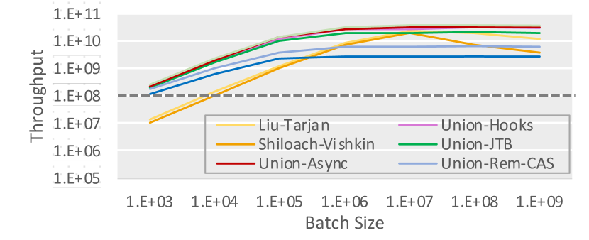
The other min-based algorithms are much slower than the union-find algorithms because the other min-based algorithms inspect more edges. In particular, $\mathsf{Liu\mathchar 45\relax Tarjan}$ is 2.86x slower on average than $\mathsf{Union\mathchar 45\relax Async}$ , and $\mathsf{Shiloach\mathchar 45\relax Vishkin}$ is 4.87x slower on average than $\mathsf{Union\mathchar 45\relax Async}$ .

Throughput vs. Batch Size. Figure 8 shows the throughput of the fastest variant for each algorithm with respect to different batch sizes. When the batch size is small, the performance significantly degrades mainly due to the GPU kernel launch overhead: the time to launch the GPU kernel takes tens of times longer than the time to run it for a small batch size. For small batch sizes, the $\mathsf{Liu\mathchar 45\relax Tarjan}$ and $\mathsf{Shiloach\mathchar 45\relax Vishkin}$ algorithms are much slower because for each batch, the GPU kernels are launched multiple times to process the current batch until the $\mathit{labels}$ array converges.

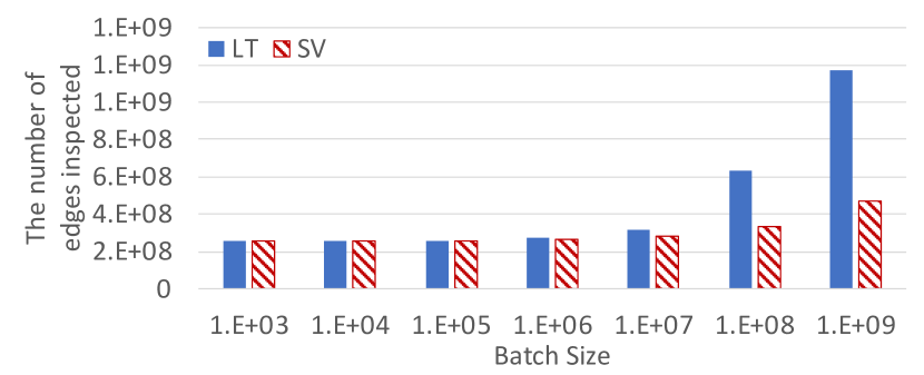
One interesting point is that $\mathsf{Liu\mathchar 45\relax Tarjan}$ and $\mathsf{Shiloach\mathchar 45\relax Vishkin}$ become slower when the batch size is larger than $10^{7}$ due to the increase in the number of edge inspections. Figure 9 shows the number of edges being inspected for different batch sizes for one variant ( $\mathsf{PRS}$ , described in Appendix A.4) of $\mathsf{Liu\mathchar 45\relax Tarjan}$ as well as $\mathsf{Shiloach\mathchar 45\relax Vishkin}$ on com-Orkut. The number of edges examined increases significantly for a batch size larger than $10^{7}$ because in those algorithms, all edges in a batch need to be inspected until the batch converges. 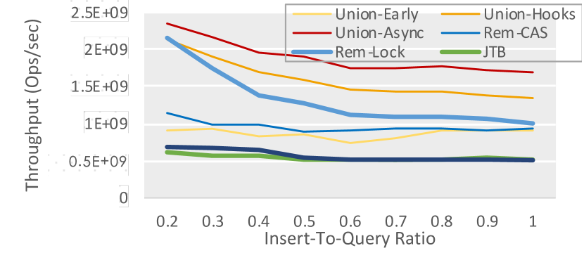We observed a similar trend in the other graphs for all variants of $\mathsf{Liu\mathchar 45\relax Tarjan}$ as well as $\mathsf{Shiloach\mathchar 45\relax Vishkin}$ .

Mixed Inserts and Queries. We evaluate the performance of the variants used in Figure 8 to study how the ratio of insertions to queries affects the throughput. For a ratio of insertions to queries of $x$ , we generate $1/x$ queries with random vertex pairs per insert, and shuffle them with the original edges (which are insertions) that are also randomly permuted to prevent data locality from affecting performance.

Figure 10 shows the throughput with different insert-to-query ratios on the europe_osm graph. As the ratio decreases, throughput also increases because the path to the root vertex in the $\mathit{labels}$ array is compressed, which speeds up the processing of the remaining insertions and queries. Note that for very well connected graphs (e.g., com-Orkut), the throughput with respect to different ratios is quite stable, because even when the ratio is 1, the labels have converged after processing a small subset of insertions.

4.5. Evaluation on Titan Xp (Pascal)

Algorithm	Average slowdown against V100		Average speedup over state-of-the-art
Algorithm	Across all variants	Fastest variants	Average speedup over state-of-the-art
Static conn.	1.62	1.71	2.38
Span. forest	1.59	1.60	–
Streaming conn.	1.79	2.25	–

Table 5. Summary of results on the Titan Xp machine.

This section presents our evaluation of $\mathsf{GConn}$ on the Titan Xp (Pascal) GPU. Table 5 shows the average slowdown against our evaluation on the V100 GPU, as well as the average of the speedup over the fastest one among $\mathsf{GPU\mathchar 45\relax CC}$ , $\mathsf{GSWITCH}$ , $\mathsf{ECL\mathchar 45\relax CC}$ , and $\mathsf{Afforest}$ also run on the Titan Xp GPU. As shown in Table 5, the trends for both GPU machines are very similar, and except for incremental connectivity, the average slowdown is close to the ratio of the bandwidth of the V100 to that of Titan Xp ( $900/547.6=1.6$ ). For incremental connectivity, accessing the $\mathit{labels}$ array requires spin-locks, which prevents the algorithms from fully saturating the memory bandwidth. We note that we had to modify $\mathsf{Union\mathchar 45\relax Rem\mathchar 45\relax Lock}$ to avoid deadlocks (O’Neil et al., 2011; Jason and Edward, 2010) for the Pascal machine in which threads in a warp are executed in lock-step (Jia et al., 2018).

4.6. Performance analysis on CPUs vs. GPUs

In this section, we compare the performance of $\mathsf{GConn}$ (Dhulipala et al., 2020b) on the V100 with the performance of $\mathsf{ConnectIt}$ . $\mathsf{ConnectIt}$ ’s experiments were performed on a Dell PowerEdge R930 with 4 $\times$ 2.4GHz Intel 18-core E7-8864 x4 Xeon professors, a 45MB L3 Cache and a memory bandwidth of 85 GB/sec.

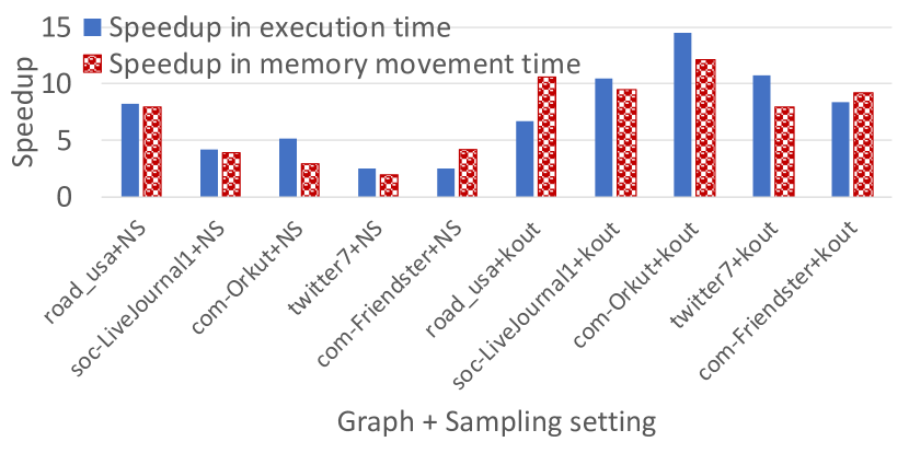
We compare CPU and GPU performance with the five graphs used in $\mathsf{ConnectIt}$ that can fit in the GPU memory (Dhulipala et al., 2020b). To understand the relation between the execution time and the total data movement from/to memory, Figure 11 shows the speedup in execution time achieved by $\mathsf{GConn}$ over $\mathsf{ConnectIt}$ (blue bars), and the speedup in time for the data movement from/to memory at peak memory bandwidth using the GPU compared to the CPU (red bars). Our GPU provides $900/85=10.59$ times higher memory bandwidth compared to the CPU, but the CPU L3 cache is much larger than the GPU L2 cache. Hence, there can be more memory transactions on the GPU, depending on the graph. As shown in Figure 11, there is a strong correlation between the execution time and the time for data movement (a Pearson correlation coefficient of $0.854$ ). Note that the first five pairs of bars are without sampling, and the rest of them are with $k$ -out sampling. For a fair comparison, we did not apply HB sampling because the best variants in $\mathsf{ConnectIt}$ for these graphs always adopt $k$ -out sampling. The best variant of $\mathsf{GConn}$ without HB sampling achieves 8.26–14.51x speedup over the best variant with $\mathsf{ConnectIt}$ . For incremental algorithms, when we treat all of the edges as one large batch, $\mathsf{GConn}$ only achieves 1.85–13.36x speedup over $\mathsf{ConnectIt}$ due to the spin-locks on the $\mathit{labels}$ array being more expensive on GPUs than CPUs.

To obtain a rough estimate of the monetary cost savings for running the connectivity algorithms on the GPU vs. the CPU, we compare two machines on Amazon EC2: the p3.2xlarge configuration, which is very similar to our V100 setup, and the x1.16xlarge configuration, which provides a multicore similar to the Dell PowerEdge R930. On-demand pricing of the p3.2xlarge and x1.16xlarge instances is $3.06 and $6.669 per hour, respectively. The fastest variant of $\mathsf{GConn}$ is 12.02x faster on average than that of $\mathsf{ConnectIt}$ . Hence, for our input graphs, we can expect to save roughly a factor of $(6.669/3.06)\times 12.02=26.2$ in costs by using a similar GPU compared to a similar CPU.

4.7. Takeaways and Guidelines

Based on our experimental study, we found that variants of union-find that have not been studied in prior work on GPU connectivity performed the best. We discovered that the sampling phase mostly dominates the execution time, which indicates that reducing the overhead for the sampling phase is crucial for high performance. We found that many of our static connectivity algorithms can be extended to support spanning forest and incremental connectivity, and can achieve high performance as well. Finally, we found GPUs to be a cost-efficient option for connectivity algorithms compared to CPUs, as long as the graph can fit in the GPU memory.

The fastest implementation is dependent on a given input graph, and as $\mathsf{GConn}$ supports several hundred variants, trying all variants to find the fastest one can be overwhelming. We provide some guidelines below on how to choose an implementation with high performance.

First, a practitioner can simply use the best variant overall based on our experimental evaluation, which is to use $\mathsf{Union\mathchar 45\relax Async}$ or $\mathsf{Union\mathchar 45\relax Rem\mathchar 45\relax CAS}$ combined with $k$ -out sampling. For our input graphs, using this approach achieves performance that is within 20.8% on average of the performance of the fastest implementation for each graph.

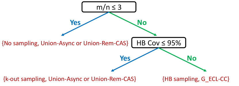
A more sophisticated dynamic mechanism for selecting sampling methods for a fixed finish method is as follows. First, we observed that if the average degree in the graph is small enough, most edges are inspected in the sampling phase, and an additional overhead to access the edge array multiple times is incurred. Therefore, we found that when the average degree is small, sampling is not a worthwhile optimization. Second, we observed that one does not need to consider BFS sampling, as it is always outperformed by either $k$ -out sampling or hook-based search (HB) sampling. From Table 3, we see that when HB Cov (the percentage of vertices in the largest connected component after HB sampling) is high enough, HB sampling is always the best strategy. As shown in Figure 6, in this case, HB sampling samples a minimal number of edges. A rough lower bound of HB Cov can be obtained by applying the first step of HB for a few edges, which is inexpensive, and then using this value to choose between HB or $k$ -out sampling.

Our study also provides insights on choosing finish methods that complement a particular sampling method. First, we found that the fastest finish method is always one of $\{$ $\mathsf{Union\mathchar 45\relax Async}$ , $\mathsf{Union\mathchar 45\relax Rem\mathchar 45\relax}$ $\mathsf{CAS}$ , or $\mathsf{G\_ECL\mathchar 45\relax CC}$ $\}$ . In the no-sampling setting, either $\mathsf{Union\mathchar 45\relax}$ $\mathsf{Async}$ or $\mathsf{Union\mathchar 45\relax Rem\mathchar 45\relax CAS}$ is the fastest. $\mathsf{G\_ECL\mathchar 45\relax CC}$ performs fewer on-the-fly compressions, which normally leads to more path traversal (and thus more cache misses). On the other hand, when HB sampling is used, which implies the input graph is very well connected, $\mathsf{G\_ECL\mathchar 45\relax CC}$ is recommended as only a very few edges are inspected by the union-find algorithms. In this case, $\mathsf{G\_ECL\mathchar 45\relax CC}$ has the lowest overhead as it does not perform much on-the-fly compression, which requires performing additional writes. On our input graphs, using this strategy for choosing the sampling and finish methods gives a slowdown of only 9.4% on average compared to using the fastest implementation for each graph.

Figure 12 presents a decision tree for the strategy above. HB Cov is the lower bound mentioned above, and $\mathsf{Union\mathchar 45\relax Async}$ can be substituted with $\mathsf{Union\mathchar 45\relax Rem\mathchar 45\relax CAS}$ as their performance is similar.

5. Conclusion

We have designed the $\mathsf{GConn}$ framework, which supports several hundred efficient implementations on GPUs for static connectivity, spanning forest, and incremental connectivity. To the best of our knowledge, this paper provides the most comprehensive study of different variants of connectivity algorithms on GPUs. Extensive evaluations show that the best connectivity implementations in $\mathsf{GConn}$ significantly outperform other state-of-the-art libraries and implementations. For future work, we are interested in extending our framework to the multi-GPU or distributed memory settings.

Acknowledgements

We thank the reviewers of this paper for their helpful feedback. This research was supported by DOE Early Career Award #DE-SC0018947, NSF CAREER Award #CCF-1845763, Google Faculty Research Award, DARPA SDH Award #HR0011-18-3-0007, and Applications Driving Architectures (ADA) Research Center, a JUMP Center co-sponsored by SRC and DARPA.

References

(1)
Acar et al. (2019) Umut A. Acar, Daniel Anderson, Guy E. Blelloch, and Laxman Dhulipala. 2019. Parallel Batch-Dynamic Graph Connectivity. In ACM Symposium on Parallelism in Algorithms and Architectures (SPAA). 381–392.
Andoni et al. (2018) Alexandr Andoni, Zhao Song, Clifford Stein, Zhengyu Wang, and Peilin Zhong. 2018. Parallel graph connectivity in log diameter rounds. In IEEE Symposium on Foundations of Computer Science (FOCS). 674–685.
Awerbuch and Shiloach (1987) B. Awerbuch and Y. Shiloach. 1987. New Connectivity and MSF Algorithms for Shuffle-Exchange Network and PRAM. IEEE Trans. Comput. C-36, 10 (1987), 1258–1263.
Bader and Cong (2005) David A. Bader and Guojing Cong. 2005. A fast, parallel spanning tree algorithm for symmetric multiprocessors (SMPs). Journal of Parallel and Distrib. Comput. 65, 9 (2005), 994–1006.
Bader et al. (2005) David A. Bader, Guojing Cong, and John Feo. 2005. On the Architectural Requirements for Efficient Execution of Graph Algorithms. In International Conference on Parallel Processing (ICPP). 547–556.
Bader and JaJa (1996) David A. Bader and Joseph JaJa. 1996. Parallel Algorithms for Image Histogramming and Connected Components with an Experimental Study. J. Parallel Distrib. Comput. 35, 2 (1996), 173–190.
Banerjee and Kothapalli (2011) Dip Sankar Banerjee and Kishore Kothapalli. 2011. Hybrid Algorithms for List Ranking and Graph Connected Components. In International Conference on High Performance Computing (HiPC). 1–10.
Barabasi and Bonabeau (2003) Albert-Laszlo Barabasi and Eric Bonabeau. 2003. Scale-Free Networks. Scientific American (2003).
Beamer et al. (2012) Scott Beamer, Krste Asanovic, and David Patterson. 2012. Direction-optimizing breadth-first search. In ACM/IEEE International Conference for High Performance Computing, Networking, Storage and Analysis (SC). Article 12, 12:1–12:10 pages.
Beamer et al. (2015) Scott Beamer, Krste Asanovic, and David A. Patterson. 2015. The GAP Benchmark Suite. CoRR abs/1508.03619 (2015). http://arxiv.org/abs/1508.03619
Behnezhad et al. (2019a) Soheil Behnezhad, Laxman Dhulipala, Hossein Esfandiari, Jakub Lacki, and Vahab Mirrokni. 2019a. Near-optimal massively parallel graph connectivity. In IEEE Symposium on Foundations of Computer Science (FOCS). 1615–1636.
Behnezhad et al. (2019b) Soheil Behnezhad, Laxman Dhulipala, Hossein Esfandiari, Jakub Lacki, Vahab Mirrokni, and Warren Schudy. 2019b. Massively Parallel Computation via Remote Memory Access. In ACM Symposium on Parallelism in Algorithms and Architectures (SPAA). 59–68.
Ben-Nun et al. (2017) Tal Ben-Nun, Michael Sutton, Sreepathi Pai, and Keshav Pingali. 2017. Groute: An Asynchronous Multi-GPU Programming Model for Irregular Computations. In ACM SIGPLAN Symposium on Principles and Practice of Parallel Programming (PPoPP). 235–248.
Blelloch et al. (2012) Guy E. Blelloch, Jeremy T. Fineman, Phillip B. Gibbons, and Julian Shun. 2012. Internally Deterministic Parallel Algorithms Can Be Fast. In ACM SIGPLAN Symposium on Proceedings of Principles and Practice of Parallel Programming (PPoPP). 181–192.
Bus and Tvrdik (2001) Libor Bus and Pavel Tvrdik. 2001. A Parallel Algorithm for Connected Components on Distributed Memory Machines. In Recent Advances in Parallel Virtual Machine and Message Passing Interface. 280–287.
Busato et al. (2018) Federico Busato, Oded Green, Nicola Bombieri, and David A Bader. 2018. Hornet: An efficient data structure for dynamic sparse graphs and matrices on GPUs. In IEEE High Performance Extreme Computing Conference (HPEC). 1–7.
Caceres et al. (2004) E.N. Caceres, F. Dehne, H. Mongelli, S.W. Song, and J.L. Szwarcfiter. 2004. A Coarse-Grained Parallel Algorithm for Spanning Tree and Connected Components. In Euro-Par.
Catanzaro et al. (2014) Bryan Catanzaro, Alexander Keller, and Michael Garland. 2014. A Decomposition for In-Place Matrix Transposition. In ACM SIGPLAN Symposium on Principles and Practice of Parallel Programming (PPoPP). 193–206.
Chakrabarti et al. (2004) Deepayan Chakrabarti, Yiping Zhan, and Christos Faloutsos. 2004. R-MAT: A Recursive Model for Graph Mining. In SIAM International Conference on Data Mining (SDM). 442–446.
Chin et al. (1982) Francis Y. Chin, John Lam, and I-Ngo Chen. 1982. Efficient Parallel Algorithms for Some Graph Problems. Commun. ACM 25, 9 (Sept. 1982), 659–665.
Chitnis et al. (2013) Laukik Chitnis, Anish Das Sarma, Ashwin Machanavajjhala, and Vibhor Rastogi. 2013. Finding Connected Components in Map-Reduce in Logarithmic Rounds. In IEEE International Conference on Data Engineering (ICDE). 50–61.
Chong and Lam (1995) K.W. Chong and T.W. Lam. 1995. Finding Connected Components in $O(\log n\log\log n)$ Time on the EREW PRAM. Journal of Algorithms 18, 3 (1995), 378–402.
Cole and Vishkin (1991) Richard Cole and Uzi Vishkin. 1991. Approximate parallel scheduling. II. Applications to logarithmic-time optimal parallel graph algorithms. Information and Computation 92, 1 (1991), 1–47.
Cong and Muzio (2014) Guojing Cong and Paul Muzio. 2014. Fast Parallel Connected Components Algorithms on GPUs. In Euro-Par. 153–164.
Cormen et al. (2009) Thomas H. Cormen, Charles E. Leiserson, Ronald L. Rivest, and Clifford Stein. 2009. Introduction to Algorithms (3. ed.). MIT Press.
Davis and Hu (2011) Timothy A. Davis and Yifan Hu. 2011. The University of Florida Sparse Matrix Collection. ACM Trans. Math. Software 38, 1 (Nov. 2011), 1:1–1:25.
Dhulipala et al. (2018) Laxman Dhulipala, Guy E. Blelloch, and Julian Shun. 2018. Theoretically Efficient Parallel Graph Algorithms Can Be Fast and Scalable. In ACM Symposium on Parallelism in Algorithms and Architectures (SPAA). 393–404.
Dhulipala et al. (2020a) Laxman Dhulipala, David Durfee, Janardhan Kulkarni, Richard Peng, Saurabh Sawlani, and Xiaorui Sun. 2020a. Parallel Batch-Dynamic Graphs: Algorithms and Lower Bounds. In ACM-SIAM Symposium on Discrete Algorithms (SODA). 1300–1319.
Dhulipala et al. (2020b) Laxman Dhulipala, Changwan Hong, and Julian Shun. 2020b. ConnectIt: A framework for static and incremental parallel graph connectivity algorithms. https://arxiv.org/abs/2008.03909
Ediger et al. (2012) D. Ediger, R. McColl, J. Riedy, and D. A. Bader. 2012. STINGER: High performance data structure for streaming graphs. In IEEE Conference on High Performance Extreme Computing (HPEC). 1–5.
Elhamifar and Vidal (2013) Ehsan Elhamifar and Rene Vidal. 2013. Sparse subspace clustering: Algorithm, theory, and applications. IEEE Transactions on Pattern Analysis and Machine Intelligence 35, 11 (2013), 2765–2781.
ElTantawy and Aamodt (2018) Ahmed ElTantawy and Tor M Aamodt. 2018. Warp scheduling for fine-grained synchronization. In IEEE International Symposium on High Performance Computer Architecture (HPCA). 375–388.
Ester et al. (1996) Martin Ester, Hans-Peter Kriegel, Jörg Sander, and Xiaowei Xu. 1996. A Density-based Algorithm for Discovering Clusters a Density-based Algorithm for Discovering Clusters in Large Spatial Databases with Noise. In International Conference on Knowledge Discovery and Data Mining (KDD). 226–231.
Gazit (1991) Hillel Gazit. 1991. An Optimal Randomized Parallel Algorithm for Finding Connected Components in a Graph. SIAM J. Comput. 20, 6 (Dec. 1991), 1046–1067.
Green and Bader (2016) O. Green and D. A. Bader. 2016. cuSTINGER: Supporting dynamic graph algorithms for GPUs. In IEEE High Performance Extreme Computing Conference (HPEC). 1–6.
Greiner (1994) John Greiner. 1994. A Comparison of Parallel Algorithms for Connected Components. In ACM Symposium on Parallelism in Algorithms and Architectures (SPAA). 16–25.
Halperin and Zwick (1994) Shay Halperin and Uri Zwick. 1994. An Optimal Randomized Logarithmic Time Connectivity algorithm for the EREW PRAM (Extended Abstract). In ACM Symposium on Parallelism in Algorithms and Architectures (SPAA).
Hambrusch and TeWinkel (1988) S. Hambrusch and L. TeWinkel. 1988. A study of connected component labeling algorithms on the MPP. In International Conference on Supercomputing (ICS). 477–483.
Han and Wagner (1990) Yujie Han and Robert A. Wagner. 1990. An Efficient and Fast Parallel-connected Component Algorithm. J. ACM 37, 3 (July 1990), 626–642.
Hawick et al. (2010) K. A. Hawick, A. Leist, and D. P. Playne. 2010. Parallel Graph Component Labelling with GPUs and CUDA. Parallel Comput. 36, 12 (Dec. 2010), 655–678.
Haythornthwaite (2005) Caroline Haythornthwaite. 2005. Social networks and Internet connectivity effects. Information, Community & Society 8, 2 (2005), 125–147.
Hirschberg et al. (1979) D. S. Hirschberg, A. K. Chandra, and D. V. Sarwate. 1979. Computing Connected Components on Parallel Computers. Commun. ACM 22, 8 (Aug. 1979), 461–464.
Ho et al. (2003) Jeffrey Ho, Ming-Husang Yang, Jongwoo Lim, Kuang-Chih Lee, and David Kriegman. 2003. Clustering appearances of objects under varying illumination conditions. In IEEE Computer Society Conference on Computer Vision and Pattern Recognition, Vol. 1.
Holm et al. (2019) J. Holm, V. King, M. Thorup, O. Zamir, and U. Zwick. 2019. Random $k$ -out Subgraph Leaves only $O(n/k)$ Inter-Component Edges. In IEEE Symposium on Foundations of Computer Science (FOCS). 896–909.
Hong et al. (2020) Changwan Hong, Laxman Dhulipala, and Julian Shun. 2020. Exploring the Design Space of Static and Incremental Graph Connectivity Algorithms on GPUs. arXiv preprint.
Hsu et al. (1997) Tsan-Sheng Hsu, Vijaya Ramachandran, and Nathaniel Dean. 1997. Parallel Implementation of Algorithms for Finding Connected Components in Graphs. In Parallel Algorithms: 3rd DIMACS Implementation Challenge. 23–41.
Iverson et al. (2015) J. Iverson, C. Kamath, and G. Karypis. 2015. Evaluation of Connected-component Labeling Algorithms for Distributed-memory Systems. Parallel Comput. 44, C (May 2015), 53–68.
Iwama and Kambayashi (1994) Kazuo Iwama and Yahiko Kambayashi. 1994. A Simpler Parallel Algorithm for Graph Connectivity. J. Algorithms 16, 2 (March 1994), 190–217.
Jaiganesh and Burtscher (2018) Jayadharini Jaiganesh and Martin Burtscher. 2018. A High-performance Connected Components Implementation for GPUs. In International Symposium on High-Performance Parallel and Distributed Computing (HPDC). 92–104.
Jain et al. (2017) C. Jain, P. Flick, T. Pan, O. Green, and S. Aluru. 2017. An Adaptive Parallel Algorithm for Computing Connected Components. IEEE Transactions on Parallel and Distributed Systems 28, 9 (2017), 2428–2439.
Jason and Edward (2010) Sanders Jason and Kandrot Edward. 2010. CUDA by example: an introduction to general-purpose GPU programming. Addison-Wesley Professional (2010).
Jayanti and Tarjan (2016) Siddhartha V. Jayanti and Robert E. Tarjan. 2016. A Randomized Concurrent Algorithm for Disjoint Set Union. In ACM Symposium on Principles of Distributed Computing (PODC). 75–82.
Jayanti et al. (2019) Siddhartha V. Jayanti, Robert E. Tarjan, and Enric Boix-Adserà. 2019. Randomized Concurrent Set Union and Generalized Wake-Up. In ACM Symposium on Principles of Distributed Computing (PODC). 187–196.
Jia et al. (2018) Zhe Jia, Marco Maggioni, Benjamin Staiger, and Daniele P Scarpazza. 2018. Dissecting the NVIDIA Volta GPU architecture via microbenchmarking. arXiv preprint arXiv:1804.06826 (2018).
Johnson and Metaxas (1997) Donald B Johnson and Panagiotis Metaxas. 1997. Connected Components in $O(\log^{3/2}n)$ Parallel Time for the CREW PRAM. J. Comput. System Sci. 54, 2 (1997), 227–242.
Karger et al. (1999) David R. Karger, Noam Nisan, and Michal Parnas. 1999. Fast Connected Components Algorithms for the EREW PRAM. SIAM J. Comput. 28, 3 (Feb. 1999), 1021–1034.
Kiveris et al. (2014) Raimondas Kiveris, Silvio Lattanzi, Vahab Mirrokni, Vibhor Rastogi, and Sergei Vassilvitskii. 2014. Connected Components in MapReduce and Beyond. In Proceedings of the ACM Symposium on Cloud Computing (SOCC). Article 18, 18:1–18:13 pages.
Koubek and Krsnakova (1985) Vaclav Koubek and Jana Krsnakova. 1985. Parallel algorithms for connected components in a graph. In Fundamentals of Computation Theory. 208–217.
Kruskal et al. (1990) Clyde P. Kruskal, Larry Rudolph, and Marc Snir. 1990. Efficient parallel algorithms for graph problems. Algorithmica 5, 1-4 (1990), 43–64.
Leskovec and Krevl (2019) Jure Leskovec and Andrej Krevl. 2019. SNAP Datasets: Stanford Large Network Dataset Collection. http://snap.stanford.edu/data.
Li and Behjat (2006) Jianhua Li and Laleh Behjat. 2006. A connectivity based clustering algorithm with application to VLSI circuit partitioning. IEEE Transactions on Circuits and Systems II: Express Briefs 53, 5 (2006), 384–388.
Liu and Tarjan (2019) Sixue Liu and Robert E. Tarjan. 2019. Simple Concurrent Labeling Algorithms for Connected Components. In Symposium on Simplicity in Algorithms (SOSA). 3:1–3:20.
Madduri and Bader (2009) Kamesh Madduri and David A. Bader. 2009. Compact graph representations and parallel connectivity algorithms for massive dynamic network analysis. In IEEE International Parallel and Distributed Processing Symposium (IPDPS). 1–11.
McColl et al. (2013) R. McColl, O. Green, and D. A. Bader. 2013. A new parallel algorithm for connected components in dynamic graphs. In IEEE International Conference on High Performance Computing (HiPC). 246–255.
Meng et al. (2019) Ke Meng, Jiajia Li, Guangming Tan, and Ninghui Sun. 2019. A Pattern Based Algorithmic Autotuner for Graph Processing on GPUs. In ACM SIGPLAN Symposium on Principles and Practice of Parallel Programming (PPoPP). 201–213.
Merrill et al. (2012) Duane Merrill, Michael Garland, and Andrew Grimshaw. 2012. Scalable GPU Graph Traversal. In ACM SIGPLAN Symposium on Principles and Practice of Parallel Programming (PPoPP). 117–128.
Nath and Maheshwari (1982) Dhruva Nath and S. N. Maheshwari. 1982. Parallel Algorithms for the Connected Components and Minimal Spanning Tree Problems. Inf. Process. Lett. 14, 1 (1982), 7–11.
Nguyen et al. (2013a) Donald Nguyen, Andrew Lenharth, and Keshav Pingali. 2013a. A Lightweight Infrastructure for Graph Analytics. In ACM Symposium on Operating Systems Principles (SOSP). 456–471.
Nguyen et al. (2013b) Donald Nguyen, Andrew Lenharth, and Keshav Pingali. 2013b. A Lightweight Infrastructure for Graph Analytics. In ACM Symposium on Operating Systems Principles (SOSP). 456–471.
O’Neil et al. (2011) Molly A O’Neil, Dan Tamir, and Martin Burtscher. 2011. A parallel GPU version of the traveling salesman problem. In Proceedings of the International Conference on Parallel and Distributed Processing Techniques and Applications (PDPTA). The Steering Committee of The World Congress in Computer Science, Computer Engineering and Applied Computing (WorldComp), 348–353.
Pai and Pingali (2016) Sreepathi Pai and Keshav Pingali. 2016. A Compiler for Throughput Optimization of Graph Algorithms on GPUs. In ACM SIGPLAN International Conference on Object-Oriented Programming, Systems, Languages, and Applications (OOPSLA). 1–19.
Patwary et al. (2012a) M. M. A. Patwary, D. Palsetia, A. Agrawal, W. k. Liao, F. Manne, and A. Choudhary. 2012a. A new scalable parallel DBSCAN algorithm using the disjoint-set data structure. In ACM/IEEE International Conference on High Performance Computing, Networking, Storage and Analysis (SC). 62:1–62:11.
Patwary et al. (2012b) Md. Mostofa Ali Patwary, Peder Refsnes, and Fredrik Manne. 2012b. Multi-core Spanning Forest Algorithms using the Disjoint-set Data Structure. In IEEE International Parallel and Distributed Processing Symposium (IPDPS). 827–835.
Phillips (1989) C. A. Phillips. 1989. Parallel Graph Contraction. In ACM Symposium on Parallelism in Algorithms and Architectures (SPAA). 148–157.
Reif (1985) J. H. Reif. 1985. Optimal Parallel Algorithms for Integer Sorting and Graph Connectivity. TR-08-85, Harvard University (1985).
Sengupta and Song (2017) Dipanjan Sengupta and Shuaiwen Leon Song. 2017. EvoGraph: On-the-Fly Efficient Mining of Evolving Graphs on GPU. In High Performance Computing. 97–119.
Shiloach and Vishkin (1982) Yossi Shiloach and Uzi Vishkin. 1982. An $O(\log n)$ Parallel Connectivity Algorithm. J. Algorithms 3, 1 (1982), 57–67.
Shun and Blelloch (2013) Julian Shun and Guy E. Blelloch. 2013. Ligra: A Lightweight Graph Processing Framework for Shared Memory. In ACM SIGPLAN Symposium on Principles and Practice of Parallel Programming (PPoPP). 135–146.
Shun et al. (2014) Julian Shun, Laxman Dhulipala, and Guy E. Blelloch. 2014. A Simple and Practical Linear-Work Parallel Algorithm for Connectivity. In ACM Symposium on Parallelism in Algorithms and Architectures (SPAA). 143–153.
Simsiri et al. (2017) Natcha Simsiri, Kanat Tangwongsan, Srikanta Tirthapura, and Kun‐Lung Wu. 2017. Work-efficient parallel union-find. Concurrency and Computation: Practice and Experience 30, 4 (2017).
Slota et al. (2014) George M. Slota, Sivasankaran Rajamanickam, and Kamesh Madduri. 2014. BFS and Coloring-based Parallel Algorithms for Strongly Connected Components and Related Problems. In IEEE International Parallel and Distributed Processing Symposium (IPDPS). 550–559.
Soman et al. (2010) J. Soman, K. Kishore, and P. J. Narayanan. 2010. A fast GPU algorithm for graph connectivity. In IEEE International Parallel and Distributed Processing Symposium (IPDPS). 1–8.
Stergiou et al. (2018) Stergios Stergiou, Dipen Rughwani, and Kostas Tsioutsiouliklis. 2018. Shortcutting Label Propagation for Distributed Connected Components. In ACM International Conference on Web Search and Data Mining (WSDM). 540–546.
Sung et al. (2014) I-Jui Sung, Juan Gómez-Luna, José María González-Linares, Nicolás Guil, and Wen-Mei W Hwu. 2014. In-place transposition of rectangular matrices on accelerators. In ACM SIGPLAN Symposium on Principles and Practice of Parallel Programming (PPoPP). 207–218.
Sutton et al. (2018) M. Sutton, T. Ben-Nun, and A. Barak. 2018. Optimizing Parallel Graph Connectivity Computation via Subgraph Sampling. In IEEE International Parallel and Distributed Processing Symposium (IPDPS). 12–21.
Tarjan and Vishkin (1985) Robert E Tarjan and Uzi Vishkin. 1985. An efficient parallel biconnectivity algorithm. SIAM J. Comput. 14, 4 (1985), 862–874.
Vishkin (1984) Uzi Vishkin. 1984. An optimal parallel connectivity algorithm. Discrete Applied Mathematics 9, 2 (1984), 197–207.
Wang et al. (2016) Yangzihao Wang, Andrew Davidson, Yuechao Pan, Yuduo Wu, Andy Riffel, and John D. Owens. 2016. Gunrock: A High-performance Graph Processing Library on the GPU. In ACM SIGPLAN Symposium on Principles and Practice of Parallel Programming (PPoPP).
Wang et al. (2017) Yangzihao Wang, Yuechao Pan, Andrew Davidson, Yuduo Wu, Carl Yang, Leyuan Wang, Muhammad Osama, Chenshan Yuan, Weitang Liu, Andy T. Riffel, and John D. Owens. 2017. Gunrock: GPU Graph Analytics. ACM Trans. Parallel Comput. 4, 1, Article 3 (Aug. 2017), 3:1–3:49 pages.
Wen et al. (2017) Dong Wen, Lu Qin, Ying Zhang, Lijun Chang, and Xuemin Lin. 2017. Efficient structural graph clustering: an index-based approach. Proceedings of the VLDB Endowment 11, 3 (2017), 243–255.
Xu et al. (2007) Xiaowei Xu, Nurcan Yuruk, Zhidan Feng, and Thomas AJ Schweiger. 2007. Scan: a structural clustering algorithm for networks. In ACM SIGKDD International Conference on Knowledge Discovery and Data Mining (KDD). 824–833.
Zhang et al. (2019) Yongzhe Zhang, Ariful Azad, and Zhenjiang Hu. 2019. FastSV: A Distributed-Memory Connected Component Algorithm with Fast Convergence. CoRR abs/1910.05971 (2019). http://arxiv.org/abs/1910.05971

Appendix A $\mathsf{GConn}$ Pseudocode

A.1. Sampling Schemes

Here we provide the pseudocode for our sampling methods in $\mathsf{GConn}$ . Algorithm 4 provides pseudocode for the $k$ -out sampling method, with parameter $k$ . We set $k=2$ in our experiments. Algorithm 5 provides pseudocode for the HB sampling method, with parameter $N$ . We set $N=4$ in our experiments. Algorithm 6 provides pseudocode for the BFS sampling method. The BFS starts from the vertex with the highest degree in the graph.

Algorithm 4

k

-out sampling

1:procedure

k

-out-Sampling(

G(V,E),\mathit{labels},k

)

\mathit{edges}\leftarrow

\{

First edge from each vertex

\}\cup\{

Sample

k-1

edges uniformly at random from each vertex

\}

\textsc{UnionFind}(\mathit{edges},\mathit{labels})

4: Fully compress the components array in parallel.

5: return

\mathit{labels}

Algorithm 5 HB sampling

1:procedure HB-Sampling(

G(V,E),\mathit{labels},N

)

\mathit{labels}\leftarrow\{\mathit{labels}[v]\leftarrow\min(v,w)\ |\ v\in V\}

\triangleright

w

is the smallest neighbor of

v

\mathit{edges}\leftarrow

\{

First

N

edges from each vertex

v

such that

\mathit{labels[v]}\neq v

\}

\textsc{UnionFind}(\mathit{edges},\mathit{labels})

5: Fully compress the components array in parallel.

6: return

\mathit{labels}

Algorithm 6 BFS sampling

1:procedure BFS-Sampling(

G(V,E),\mathit{labels}

)

s\leftarrow\operatorname{argmax}_{v\in V_{s}}d(v)

\triangleright

V_{s}

is a sampled subset of

V

\mathit{labels}\leftarrow\textsc{LabelSpreadingBFS}(G,s)

\mathit{freq}\leftarrow\textsc{IdentifyFrequent}(\mathit{labels})

5: return

\mathit{labels}

Algorithm 7

\mathsf{Connectivity(Union\mathchar 45\relax Find)}

\mathsf{FindOption}=\{

\triangleright

Shared by union-find algorithms

\mathsf{Naive}{}

\triangleright

No path compression

\mathsf{AtomicSplit}{}

\triangleright

Path splitting

\mathsf{TwoTrySplit}{}

\triangleright

Two-try splitting (only for

\mathsf{\mathsf{Union\mathchar 45\relax JTB}{}}

)

\mathsf{AtomicHalve}{}

\triangleright

Path halving

\mathsf{Compress}{}

\triangleright

Full path compression

\}

\mathsf{SpliceOption}=\{

\triangleright

Used by Rem’s algorithms when path has not yet reached a root

\mathsf{AtomicSplitOne}{}

\triangleright

Performs one path split

10:

\mathsf{AtomicHalveOne}{}

\triangleright

Performs one path halve

11:

\mathsf{SpliceAtomic}{}

\triangleright

Performs a splice operation

12:

\}

13:

\mathsf{UnionOption}=\{

14:

\mathsf{\mathsf{Union\mathchar 45\relax Async}{}}

\triangleright

Asynchronous union-find

15:

\mathsf{\mathsf{Union\mathchar 45\relax Hooks}{}}

\triangleright

Asynchronous hook-based union-find

16:

\mathsf{\mathsf{Union\mathchar 45\relax Early}{}}

\triangleright

Union with early-optimization

17:

\mathsf{\mathsf{Union\mathchar 45\relax Rem\mathchar 45\relax Lock}{}}

\triangleright

Lock-based Rem’s algorithm

18:

\mathsf{\mathsf{Union\mathchar 45\relax Rem\mathchar 45\relax CAS}{}}

\triangleright

CAS-based Rem’s algorithm

19:

\mathsf{\mathsf{Union\mathchar 45\relax JTB}{}}

\triangleright

Randomized algorithm by Jayanti, Tarjan, and Boix-Adserà

20:

\mathsf{\mathsf{G\_ECL\mathchar 45\relax CC}{}}

\triangleright

The union-find algorithm used in

\mathsf{ECL\mathchar 45\relax CC}

21:

\mathsf{\mathsf{G\_Afforest}{}}

\triangleright

The union-find algorithm used in

\mathsf{Afforest}

22:

\}

23:procedure Connectivity(

G

\mathit{labels}

\mathit{L_{\max}}

\mathsf{UnionOption}

\mathsf{FindOption}

\mathsf{SpliceOption}

)

24:

\mathcal{U}=\mathsf{Union\mathchar 45\relax Find}(\mathsf{UnionOption}

\mathsf{FindOption}

\mathsf{SpliceOption})

25: parfor

\{u\ |\ \mathit{labels}[u]\neq\mathit{L_{\max}}\}

26: parfor

\{(u,v)\in d^{+}(u)\}

27:

\mathcal{U}.\mathsf{Union}(u,v,\mathit{labels})

Algorithm 8 Find Algorithms

1:procedure FindNaive(

u,P

)

v\leftarrow u

3: while

v\neq P[v]^{*}

v\leftarrow P[v]

5: return

v

6:procedure FindCompress(

u,P

)

r\leftarrow u

8: if

P[r]=r

then return

r

9: while

r\neq P[r]

10:

r\leftarrow P[r]

11: while

j\leftarrow P[u]>r

12:

P[u]\leftarrow r

u\leftarrow j

13: return

r

14:procedure

\mathsf{AtomicSplit}

(

u,P

)

15:

v\leftarrow P[u],w\leftarrow P[v]

16: while

v\neq w^{*}

17:

\textsc{CAS{}}(\&P[u],v,w)

18:

u\leftarrow v

19: return

v

20:procedure

\mathsf{AtomicHalve}

(

u,P

)

21:

v\leftarrow P[u],w\leftarrow P[v]

22: while

v\neq w^{*}

23:

\textsc{CAS{}}(\&P[u],v,w)

24:

u\leftarrow P[u]

25: return

v

Algorithm 9 Splice Algorithms

1:procedure

\mathsf{AtomicSplitOne}

(

u,x,P

)

v\leftarrow P[r_{u}],w\leftarrow P[v]^{*}

3: if

v\neq w

then

\textsc{CAS{}}(\&P[u],v,w)

5: return

v

6:procedure

\mathsf{AtomicHalveOne}

(

u,x,P

)

v\leftarrow P[r_{u}],w\leftarrow P[v]^{*}

8: if

v\neq w

then

\textsc{CAS{}}(\&P[u],v,w)

10: return

w

11:procedure

\mathsf{SpliceAtomic}

(

u,v,P

)

12:

p_{u}=P[u]^{*}

13:

\textsc{CAS{}}(\&P[u],p_{u},P[v])

14: return

p_{u}

A.2. Union-Find Algorithms

In this section, we provide the pseudocode for our union-find implementations. Algorithm 7 shows our generic union-find template algorithm, which takes a custom union operator, find operator, and splice operator, and runs the resulting algorithm combination. The splice operator is only valid for Rem’s algorithms. Algorithm 8 provides pseudocode for the different find implementations. Algorithm 9 provides pseudocode for the different splice options.

Next, we provide pseudocode for each of the union-find implementations in this paper, other than $\mathsf{Union\mathchar 45\relax JTB}$ , whose pseudocode is presented in their paper (Jayanti et al., 2019).

Asynchronous Union-Find. The first class of algorithms are inspired by a recent paper exploring concurrent union-find implementations by Jayanti and Tarjan (Jayanti and Tarjan, 2016). We implement all of the variants from their paper, as well as a full path compression technique (also considered in (alistarh2019search)) which works better in practice in some cases. We refer to this union-find algorithm as $\bm{\mathsf{Union\mathchar 45\relax Async}{}}$ (Algorithm 10), since it is the classic union-find algorithm directly adapted for an asynchronous shared-memory setting. The algorithm links from higher ID to lower ID vertices to avoid cycles, and only performs links on roots. This algorithm can be combined with one of the following implementations of the find operation: $\bm{\mathsf{FindNaive}}$ , which performs no compression during the operation, $\bm{\mathsf{FindSplit}}$ and $\bm{\mathsf{FindHalve}}$ , which perform path-splitting and path-halving, respectively, and $\bm{\mathsf{FindCompress}}$ , which fully compresses the find path. Jayanti and Tarjan show that this class of algorithms is linearizable for a set of concurrent union and find operations (while they do not consider $\mathsf{FindCompress}$ , it is relatively easy to show that it is linearizable). Note that in Algorithms 8–14, we mark linearization points (which define a total order of the operations and are used to verify the correctness of algorithms (Jayanti et al., 2019)) with an asterisk (e.g., Line 4 in Algorithm 8).

Algorithm 10

\mathsf{Union\mathchar 45\relax Async}

1:Find = one of

\{\mathsf{FindNaive},\mathsf{\mathsf{AtomicSplit}{}},

\mathsf{\mathsf{AtomicHalve}{}},\mathsf{FindCompress}\}

3:procedure Union(

u,v,P

)

p_{u}\leftarrow\textsc{Find}(u,P),p_{v}\leftarrow\textsc{Find}(v,P)

5: while

p_{u}\neq p_{v}

\triangleright

WLOG, let

p_{u}>p_{v}

6: if

p_{u}=P[p_{u}]

and

\textsc{CAS{}}(\&P[u],p_{u},p_{v})

then

7: return

p_{u}\leftarrow\textsc{Find}(u,P),p_{v}\leftarrow\textsc{Find}(v,P)

We also consider two similar variants of the $\mathsf{Union\mathchar 45\relax Async}$ algorithm: $\mathsf{Union\mathchar 45\relax Hooks}$ (Algorithm 11) and $\mathsf{Union\mathchar 45\relax Early}$ (Algorithm 12). $\bm{\mathsf{Union\mathchar 45\relax Hooks}{}}$ is closely related to $\mathsf{Union\mathchar 45\relax Async}$ , with the only difference between the algorithms is that instead of performing a CAS directly on the array storing the connectivity labeling, we perform a CAS on an auxiliary $\mathit{hooks}$ array, and perform an uncontended write on the $\mathit{parents}$ array. $\bm{\mathsf{Union\mathchar 45\relax Early}{}}$ is also similar to $\mathsf{Union\mathchar 45\relax Async}$ , except that the algorithm traverses the paths from both vertices together, and tries to eagerly check and hook a vertex once it is a root. The algorithm can optionally perform a find on the endpoints of the edge after the union operation finishes, which has the effect of compressing the find path. The linearizability proof for $\mathsf{Union\mathchar 45\relax Async}$ by Jayanti and Tarjan (Jayanti and Tarjan, 2016) applies almost verbatim to $\mathsf{Union\mathchar 45\relax Hooks}$ and $\mathsf{Union\mathchar 45\relax Early}$ , and shows that both algorithms are linearizable for a set of concurrent finds and unions.

Algorithm 11

\mathsf{Union\mathchar 45\relax Hooks}

1:Find = one of

\{\mathsf{FindNaive},\mathsf{\mathsf{AtomicSplit}{}},

\mathsf{\mathsf{AtomicHalve}{}},\mathsf{FindCompress}\}

\mathit{H}\leftarrow\{i\rightarrow\infty\ |\ i\in[0,\ldots,n-1]\}

\triangleright

Array of hooks

4:procedure Union(

u,v,P

)

p_{u}\leftarrow\textsc{Find}(u,P),p_{v}\leftarrow\textsc{Find}(v,P)

6: while

p_{u}\neq p_{v}

\triangleright

WLOG, let

p_{u}>p_{v}

7: if

p_{u}=P[p_{u}]

and

\textsc{CAS{}}(\&H[u],\infty,p_{v})

then

P[p_{u}]\leftarrow p_{v}

9: return

10:

p_{u}\leftarrow\textsc{Find}(u,P),p_{v}\leftarrow\textsc{Find}(v,P)

\triangleright

WLOG, let

p_{u}>p_{v}

Algorithm 12

\mathsf{Union\mathchar 45\relax Early}

1:Find = one of

\{\mathsf{FindNaive},\mathsf{\mathsf{AtomicSplit}{}},

\mathsf{\mathsf{AtomicHalve}{}},\mathsf{FindCompress}\}

3:procedure Union(

u,v,P

)

p_{u}\leftarrow u,p_{v}\leftarrow v

5: while

p_{u}\neq p_{v}

\triangleright

WLOG, let

p_{u}>p_{v}

6: if

p_{u}=P[p_{u}]

and

\textsc{CAS{}}(\&P[u],p_{u},p_{v})

then

7: break

z\leftarrow P[p_{u}],w\leftarrow P[z]

\textsc{CAS{}}(\&P[p_{u}],z,w)

10:

p_{u}\leftarrow w

11:

\textsc{Find}(u,P),\textsc{Find}(v,P)

\triangleright

Elided if the find-option is

\mathsf{FindNaive}

Concurrent Rem’s Algorithms. We implement two concurrent versions of Rem’s algorithm, a lock-based version by Patwary et al. (Patwary et al., 2012b) ( $\bm{\mathsf{UnionRemLock}}$ , shown in Algorithm 13) and a lock-free compare-and-swap based implementation ( $\bm{\mathsf{UnionRemCAS}}$ , shown in Algorithm 14). The lock-based version of Rem’s algorithm can be combined with the same rules for path compression described for $\mathsf{Union}$ above, with the exception of $\mathsf{FindCompress}$ . We also implemented another lock-based version of Rem’s algorithm to support NVIDIA GPUs before Volta generation. The CAS-based version of Rem’s algorithm takes, in addition to the same full path compression strategies as $\mathsf{UnionRemCAS}$ , an extra splice strategy, which is used when a step of the union algorithm operates at a non-root vertex. $\mathsf{UnionRemCAS}$ can be combined with one of the following rules: $\bm{\mathsf{HalveAtomicOne}}$ , $\bm{\mathsf{SplitAtomicOne}}$ , and $\bm{\mathsf{SpliceAtomic}}$ . The first two rules perform a single path-halving or path-splitting, and the second rule performs the splicing operation described in Rem’s algorithm. Rem’s algorithm is correct in a phase-concurrent setting, where unions and find queries are separated by a barrier (Dhulipala et al., 2020b).

Randomized Two-Try Splitting. Next, we incorporate a more sophisticated randomized algorithm by Jayanti, Tarjan, and Boix-Adserà (Jayanti et al., 2019), and refer to this algorithm as $\bm{\mathsf{Union\mathchar 45\relax JTB}{}}$ . The algorithm either performs finds naively, without using any path compression ( $\bm{\mathsf{FindSimple}}$ ), or uses a strategy called $\bm{\mathsf{FindTwoTrySplit}}$ , which guarantees provably efficient bounds for their algorithm, assuming a source of random bits. We give a faithful implementation of the algorithm presented by Jayanti, Jayanti, Tarjan, and Boix-Adserà (Jayanti et al., 2019), and refer to their paper for the pseudocode and proofs of correctness. The $\mathsf{Union\mathchar 45\relax JTB}$ algorithm is linearizable, and only links roots.

Algorithm 13

\mathsf{Union\mathchar 45\relax Rem\mathchar 45\relax Lock}

1:Compress = one of

\{\mathsf{FindNaive},\mathsf{\mathsf{AtomicSplit}{}},\mathsf{\mathsf{AtomicHalve}{}}\}

\mathsf{SpliceAtomic}

= one of

\{\mathsf{HalveAtomicOne},\mathsf{SplitAtomicOne},

\mathsf{SpliceAtomic}\}

\mathit{L}\leftarrow

array of

n

locks

5:procedure Union(

u,v,P

)

r_{u}\leftarrow u,r_{v}\leftarrow v

7: while

P[r_{u}]\neq P[r_{v}]^{*}

\triangleright

WLOG, let

P[r_{u}]>P[r_{v}]

8: if

r_{u}=P[r_{u}]

then

L[r_{u}].\textsc{Lock}()

10:

p_{v}\leftarrow P[r_{v}]

11: if

r_{u}=P[r_{u}]

and

r_{u}>p_{v}^{*}

then

12:

P[r_{u}]\leftarrow p_{v}

13:

L[r_{u}].\textsc{Unlock}()

14: return

\mathsf{True}

15: else

16:

r_{u}\leftarrow\textsc{$\mathsf{SpliceAtomic}${}}(r_{u},r_{v},P)

17: if

\textsc{Compress}\neq\mathsf{FindNaive}

then

18:

\textsc{Find}(u,P),\textsc{Find}(v,P)

19: return

\mathsf{False}

Algorithm 14

\mathsf{Union\mathchar 45\relax Rem\mathchar 45\relax CAS}

1:Compress = one of

\{\mathsf{FindNaive},\mathsf{\mathsf{AtomicSplit}{}},\mathsf{\mathsf{AtomicHalve}{}}\}

\mathsf{SpliceAtomic}

= one of

\{\mathsf{HalveAtomicOne},\mathsf{SplitAtomicOne},

\mathsf{SpliceAtomic}\}

4:procedure Union(

(u,v,P)

)

r_{u}\leftarrow u,r_{v}\leftarrow v

6: while

P[r_{u}]\neq P[r_{v}]^{*}

\triangleright

WLOG, let

P[r_{u}]>P[r_{v}]

7: if

r_{u}=P[r_{u}]

and

\textsc{CAS{}}(\&P[r_{u}],r_{u},P[r_{v}])^{*}

then

8: if

\textsc{Compress}\neq\mathsf{Naive}{}

then

\textsc{Compress}(u,P)

10:

\textsc{Compress}(v,P)

11: return

\mathsf{True}

12: else

13:

r_{u}\leftarrow\textsc{$\mathsf{SpliceAtomic}${}}(r_{u},r_{v},P)

14: return

\mathsf{False}

A.3. Shiloach-Vishkin Algorithm

Algorithm 15 shows the pseudocode for our adaptation of the Shiloach-Vishkin algorithm.

Algorithm 15

\mathsf{Shiloach\mathchar 45\relax Vishkin}

1:procedure Connectivity(

G

\mathit{labels}

\mathit{frequentid}

)

\mathit{changed}\leftarrow\mathsf{true}

\mathit{candidates}\leftarrow\{v\in V\ |\ \mathit{labels}[v]\neq\mathit{frequentid}\}

\mathit{prev\_labels}\leftarrow\mathit{parents}

\triangleright

A copy

5: while

\mathit{changed}=\mathsf{true}

\mathit{changed}=\mathsf{false}

7: parfor

\{v\in\mathit{candidates}\}

8: parfor

\{(u,v)\in d^{+}(u)\}

p_{u}=\mathit{labels}[u],p_{v}=\mathit{labels}[v]

10:

l=\min(p_{u},p_{v}),h=\max(p_{u},p_{v})

11: if

l\neq h

and

h=\mathit{prev\_labels}[h]

then

12:

\textsc{writeMin{}}(\&\mathit{labels}[h],l)

13:

\mathit{changed}\leftarrow\mathsf{true}

14: parfor

\{v\in V\}

15:

\textsc{FullShortcut}(v,\mathit{labels})

16:

\mathit{prev\_labels}[v]\leftarrow\mathit{parents}[v]

A.4. Liu-Tarjan Algorithms

Finally, we describe the variants of the Liu-Tarjan framework implemented in $\mathsf{GConn}$ . Liu and Tarjan provide a framework for simple and elegant concurrent connectivity algorithms based on several simple rules which manipulate an array of parent pointers using edges to transmit the connectivity information (Liu and Tarjan, 2019). These algorithms are not traditional concurrent algorithms, but actually parallel algorithms designed for the Massively Parallel Computation ( $\mathsf{MPC}$ ) setting. We implement the framework proposed in their paper as part of $\mathsf{GConn}$ , and also include several variants that can be generated by their framework but were not considered in their paper (only five variants were explored in their original paper). Their framework ensures that the parent array is a minimum labeling, where each vertex’s parent is the minimum value among messages that it has received.

Conceptually, each round of the algorithm processes all of the edges and performs several rules on each edge. In each round, each vertex receives a number of messages and updates its parent at the end of the round to the minimum message it receives. Each round performs a connect phase, an update phase, a shortcut phase, and possibly an alter phase. The connect phase has several operations. A $\mathsf{Connect}$ sends the endpoints of an edge to both vertices. A $\mathsf{ParentConnect}$ sends the parents of the endpoints of an edge to both vertices. An $\mathsf{ExtendedConnect}$ sends the parent values of an edge to the edge endpoints as well as the parents of the endpoints. Next, the framework performs the update phase, where there are two options. The first option, $\mathsf{Update}$ sets the parent of every vertex to the minimum received ID. The second option, $\mathsf{RootUpdate}$ only updates the parents of tree roots using an $\mathsf{Update}$ . Next, the framework performs the shortcut phase, which calls $\mathsf{Shortcut}$ to perform one step of path compression. The algorithm can execute an optional alter phase. $\mathsf{Alter}$ updates the endpoints of an edge to be the current labels of the endpoints, which is necessary when using $\mathsf{Connect}$ .

Below, we list all variants of the Liu-Tarjan algorithm that we consider in this paper.

(1)

$\mathsf{CUSA}$ : $\{\mathsf{Connect}{},\mathsf{Update}{},\mathsf{Shortcut}{},\mathsf{Alter}{}\}$
(2)

$\mathsf{CRSA}$ : $\{\mathsf{Connect}{},\mathsf{RootUpdate}{},\mathsf{Shortcut}{},\mathsf{Alter}{}\}$
(3)

$\mathsf{PUSA}$ : $\{\mathsf{ParentConnect}{},\mathsf{Update}{},\mathsf{Shortcut}{},\mathsf{Alter}{}\}$
(4)

$\mathsf{PRSA}$ : $\{\mathsf{ParentConnect}{},\mathsf{RootUpdate}{},\mathsf{Shortcut}{},\mathsf{Alter}{}\}$
(5)

$\mathsf{PUS}$ : $\{\mathsf{ParentConnect}{},\mathsf{Update}{},\mathsf{Shortcut}{}\}$
(6)

$\mathsf{PRS}$ : $\{\mathsf{ParentConnect}{},\mathsf{RootUpdate}{},\mathsf{Shortcut}{}\}$
(7)

$\mathsf{EUSA}$ : $\{\mathsf{ExtendedConnect}{},\mathsf{Update}{},\mathsf{Shortcut}{},\mathsf{Alter}{}\}$
(8)

$\mathsf{EUS}$ : $\{\mathsf{ExtendedConnect}{},\mathsf{Update}{},\mathsf{Shortcut}{}\}$
(9)

$\mathsf{CUFA}$ : $\{\mathsf{Connect}{},\mathsf{Update}{},\mathsf{FullShortcut}{},\mathsf{Alter}{}\}$
(10)

$\mathsf{CRFA}$ : $\{\mathsf{Connect}{},\mathsf{RootUpdate}{},\mathsf{FullShortcut}{},\mathsf{Alter}{}\}$
(11)

$\mathsf{PUFA}$ : $\{\mathsf{ParentConnect}{},\mathsf{Update}{},\mathsf{FullShortcut}{},\mathsf{Alter}{}\}$
(12)

$\mathsf{PRFA}$ : $\{\mathsf{ParentConnect}{},\mathsf{RootUpdate}{},\mathsf{FullShortcut}{},\mathsf{Alter}{}\}$
(13)

$\mathsf{PUF}$ : $\{\mathsf{ParentConnect}{},\mathsf{Update}{},\mathsf{FullShortcut}{}\}$
(14)

$\mathsf{PRF}$ : $\{\mathsf{ParentConnect}{},\mathsf{RootUpdate}{},\mathsf{FullShortcut}{}\}$
(15)

$\mathsf{EUFA}$ : $\{\mathsf{ExtendedConnect}{},\mathsf{Update}{},\mathsf{FullShortcut}{},\mathsf{Alter}{}\}$
(16)

$\mathsf{EUF}$ : $\{\mathsf{ExtendedConnect}{},\mathsf{Update}{},\mathsf{FullShortcut}{}\}$

Exploring the Design Space of Static and Incremental Graph Connectivity Algorithms on GPUs

Abstract.

1. Introduction

2. Notation, Preliminaries, and Prior Work

3. 𝖦𝖢𝗈𝗇𝗇𝖦𝖢𝗈𝗇𝗇\mathsf{GConn} Overview

3.1. Overview of 𝖢𝗈𝗇𝗇𝖾𝖼𝗍𝖨𝗍𝖢𝗈𝗇𝗇𝖾𝖼𝗍𝖨𝗍\mathsf{ConnectIt}

3.2. 𝖦𝖢𝗈𝗇𝗇𝖦𝖢𝗈𝗇𝗇\mathsf{GConn} Framework

3.3. Sampling Algorithms

3.4. Finish Algorithms

3.5. Iterative GPU Optimizations

3.6. Incremental Connectivity Support

4. Evaluation

4.1. Static Parallel Connectivity without Sampling

4.2. Static Parallel Connectivity with Sampling

4.3. Comparison with State-of-the-art

4.4. Incremental Parallel Graph Connectivity

4.5. Evaluation on Titan Xp (Pascal)

4.6. Performance analysis on CPUs vs. GPUs

4.7. Takeaways and Guidelines

5. Conclusion

Acknowledgements

References

Appendix A 𝖦𝖢𝗈𝗇𝗇𝖦𝖢𝗈𝗇𝗇\mathsf{GConn} Pseudocode

A.1. Sampling Schemes

A.2. Union-Find Algorithms

A.3. Shiloach-Vishkin Algorithm

A.4. Liu-Tarjan Algorithms

3. $\mathsf{GConn}$ Overview

3.1. Overview of $\mathsf{ConnectIt}$

3.2. $\mathsf{GConn}$ Framework

Appendix A $\mathsf{GConn}$ Pseudocode