Prospects of Indirect Detection for the Heavy S3 Dark Doublet

Abstract

We present an analysis of the Dark S3 model in the heavy DM mass region, this model features an S3 symmetric extension of the scalar sector of the SM including a scalar $SU(2)$ doublet dark matter candidate. We use publicly available tools to compute, in addition to conventional physical constraints on the parameter space of the model, the Sommerfeld enhancement factors for the present day annihilation cross section and the likelihood profile for a simulation of an observation run by the Cherenkov Telescope Array of the Coma Berenices dwarf galaxy. Our results disfavour masses above $\sim$5 TeV mainly because of overproduction of dark matter not consistent with the relic abundance observations; we also find a moderately large region with masses in between 1.2 and 4.9 TeV which predict the correct value of the DM relic and in addition have a light scalar with the characteristics of the SM Higgs boson (i.e. within the decoupling limit akin to the THDM). Comparison of our results with model independent exclusion curves from HESS and other CTA simulations show that these limits fall short only an order of magnitude in the value of the annihilation cross section in order to exclude the best fit point of the model.

1 Introduction

The study of extensions of the Standard Model (SM) capable of tackling one or more of the well known issues present in this paradigm of particle physics continues to be one of the most active fields of contemporary research. One strategy is to approach the subject from the scalar sector of the SM, enlarging its field content with extra scalars while keeping the rest of the sectors untouched. As demonstrated by the vast literature on the Two Higgs Doublet Model (THDM), the simplest of such extensions, the possibility of stumbling into rich and interesting phenomenology is just around the corner (see e.g. [1] and references therein). Moreover, by taking the extra scalar doublet as inert (the Inert Doublet Model (IDM) [2]) we end up with a very simple and at the same time highly illustrative model containing a candidate for dark matter with rich phenomenology, e.g. see for example [3, 4, 5, 6, 7, 8, 9, 10, 11, 12, 13, 14, 15, 16, 17, 18, 19, 20, 21, 22, 23, 24, 25, 26, 27, 28, 29, 30, 31, 32, 33, 34, 35, 36, 37].

Multihiggs models are natural generalizations of this scheme, including those with additional symmetries imposed, for example the $S3$ symmetric model where a total of three Higgs doublets are present and it is assumed that these scalars (and the matter sector) belong to irreducible representations of the permutation group $S3$ reflecting a hypothesized discrete symmetry of the model, motivated in part by the fact that matter particles of a given flavor are only distinguishable from other flavors by their masses and therefore are identical to each other before electroweak symmetry breaking (EWSB). The study of these models was pioneered in [38, 39, 40] which has led to subsequent interesting research, see e.g. [41, 42, 43, 44, 45, 46, 47, 48, 49, 50, 51, 52, 53, 54, 55, 56, 57, 58, 59].

In this letter we continue our research initiated in [53] wherein we exploit the fact that the permutation group $S3$ has four irreducible representations, this leaves just enough space to augment to the $S3$ symmetric model a fourth scalar doublet which, when taken as inert, comprises a simple IDM-like dark sector. This time, we focus our attention on the high ($1-20$ TeV) DM candidate mass region of the parameter space of the model exploring the possibilities of indirect detection (ID) of gamma ray signals specifically in the Cherenkov Telescope Array (CTA), from a simulated observation of the dwarf spheroidal galaxy Coma Berenices. In this large mass regime it is important to take into account the nonperturbative phenomenon of Sommerfeld enhancement which is a manifestation of the multiple exchanges of gauge bosons and higgses between two annihilating DM particles, specially for the correct analysis of the gamma ray fluxes predicted by the model whose detection is the holy grail of dark matter ID experiments. This phenomenon occurs because the DM particles move at present with nonrelativistic (NR) velocities ($\sim 10^{-3}$) and (colloquially speaking) they have enough time to exchange (on-shell) mediators before the actual annihilation. As a result, the wave function of the DM pair is no longer a plane wave and to correctly predict the annihilation cross section it is necessary to find out the modified wave function. This process becomes particular important when the mass of the DM candidate is much larger than the gauge bosons and higgses because then the electroweak force between the DM pair becomes “long range”, and also when there are other particles in the dark sector such as those part of the same multiplet of $SU(2)$ as the DM candidate, because then the EWSB induced mass splitting between these particles is relatively small and as a result the exchange of mediators can induce transitions of the original annihilating DM pair to other states in the multiplet, which potentially enhances the annihilation cross section.

Thus, for our analysis we compute the predicted DM annihilating gamma ray flux with Sommerfeld corrections from the mentioned dwarf galaxy and use this prediction to obtain a likelihood estimate from a simulated observation at the CTA. Specifically, we simulate a null-result experiment, meaning that we assume that during the observation period no significant gamma ray signal above background was encountered, this permits us to obtain a likelihood estimate and a test statistics (TS) from the comparison of both hypothesis, the existence or non-existence of a signal from DM annihilation, which in turn leads to the estimate of limiting or exclusion regions for the parameter space of the model. In order to obtain such information of the parameter space we perform a directed scan, for each probed point (set of values of the independent parameters) in the model we feed the predicted flux to the public CTA analysis tools obtaining a likelihood estimate and a TS, we then supplement the estimated likelihood with information regarding unitarity and collider constraints on heavy scalars as well as the comparison with the relic abundance experimental value. For simplicity, we neither reject points on account of violating unitarity or collider bounds nor define additional likelihood functions to deal with these constraints. Instead, equivalently, we simply penalize the CTA likelihood estimate when this happens as well as when the predicted relic abundance is above the experimental value, but we allow for points with relic abundance predictions below this bound to account for the possibility of under-abundant DM component. Our analysis allows us to present a likelihood profile of the parameter space of the model and estimate to what extend future observations of the CTA array can probe the model.

2 Flux from annihilating DM pairs

2.1 The model

The $S3$-model is an extension of the scalar sector of the SM with a total of three $SU(2)$ doublets which, together with the matter sector, are assumed to transform under the permutation group $S3$ in such a manner that the Lagrangian respects the symmetry even after EWSB. Two of the EW doublets, $\Phi_{1}$ and $\Phi_{2}$ are chosen to form an $S3$ doublet while the third one $\Phi_{s}$ transforms as a symmetric singlet of $S3$; the matter sector is chosen to have transformation properties as in reference [47]. We take advantage of the fact that the $S3$ group has four irreducible representations which allows us to introduce a dark sector in the model by including an extra $SU(2)$ doublet, $\Phi_{a}$, transforming as an antisymmetric singlet of $S3$ and imposing a $Z_{2}$ discrete symmetry under which the only field with nontrivial transformation is $\Phi_{a}$. The dark sector scalar potential is constructed as follows:

$$V_{\textrm{DM}}=V_{2a}+V_{4a}+V_{4sa}$$ (1)

where each term is given respectively by:

$$V_{2a}=\mu_{2}^{2}\Phi_{a}^{\dagger}\Phi_{a}$$ (2)

$$V_{4a} = \lambda_{10}(\Phi_{a}^{\dagger}\Phi_{a})(\Phi_{1}^{\dagger}\Phi_{1}+\Phi_{2}^{\dagger}\Phi_{2})$$ (3)

$$+\lambda_{11}[(\Phi_{a}^{\dagger}\Phi_{1})(\Phi_{1}^{\dagger}\Phi_{a})+(\Phi_{a}^{\dagger}\Phi_{2})(\Phi_{2}^{\dagger}\Phi_{a})]$$

$$+\lambda_{12}[(\Phi_{a}^{\dagger}\Phi_{1})(\Phi_{a}^{\dagger}\Phi_{1})+(\Phi^{\dagger}_{a}\Phi_{2})(\Phi^{\dagger}_{a}\Phi_{2})+\mathrm{h.c.}]$$

$$+\lambda_{13}(\Phi^{\dagger}_{a}\Phi_{a})^{2}$$

$$V_{4sa}=\lambda_{14}(\Phi_{s}^{\dagger}\Phi_{a}\Phi_{a}^{\dagger}\Phi_{s})$$ (4)

For the full Lagrangian and complete details of the model we refer the reader to our previous work [53], here we’ll just give some expressions not explicitly given there which we’ll use in the recount of this research. After EWSB the $Z_{2}$ even scalars acquire vacuum expectation values (vev) $v_{1}$, $v_{2}$ and $v_{s}$, but from the consistency of the minimization conditions of the scalar potential two of the vevs are aligned $v_{1}=\sqrt{3}v_{2}$. This, together with the requirement $v=\sqrt{v_{s}^{2}+4v_{2}^{2}}=$ 246 GeV, where $v$ is the SM vev leads to only one independent vev parameter, we choose $\tan{\theta}=2v_{2}/v_{s}$ as independent parameter in the numerical calculations. EWSB induces mixing between the $Z_{2}$ even scalars, the CP even ones mix through the matrix:

$$Z^{h}=\left(\begin{array}[]{ccc}\cos(\alpha)&0&\sin(\alpha)\\ 0&1&0\\ -\sin(\alpha)&0&\cos(\alpha)\\ \end{array}\right)\left(\begin{array}[]{ccc}1&0&0\\ 0&\frac{1}{2}&-\frac{\sqrt{3}}{2}\\ 0&\frac{\sqrt{3}}{2}&\frac{1}{2}\\ \end{array}\right)$$ (5)

while the charged and CP-odd scalars mix respectively with the matrices:

$$Z^{C}=Z^{A}=\left(\begin{array}[]{ccc}\cos({\theta})\sin({\theta})&0&\sin^{2}({\theta})\\ 0&1&0\\ -\cos({\theta})\sin({\theta})&0&\cos^{2}({\theta})\\ \end{array}\right)\left(\begin{array}[]{ccc}1&0&0\\ 0&\frac{1}{2}&-\frac{\sqrt{3}}{2}\\ 0&\frac{\sqrt{3}}{2}&\frac{1}{2}\\ \end{array}\right)$$ (6)

i.e. both matrices coincide. Explicit expressions for the mixing angle $\alpha$ and the masses of all the scalars can be found in [53], these are given in terms of the 15 free parameters of the model: $\lambda_{1}$ - $\lambda_{8}$, $\lambda_{10}$ - $\lambda_{14}$, $\tan{\theta}$ and $\mu_{2}$ (there are only 15 free parameters because we are assuming a simple form of the Yukawa matrices, see the above reference for details and justification). There are 10 physical scalars in the model, we use interchangeably the following two notations, $\tilde{h}_{k}$ with $k=1,2,3$ for the neutral scalars $H$, $H_{3}$ and $h$ (i.e. $\tilde{h}_{1}=H$, $\tilde{h}_{2}=H_{3}$ and $\tilde{h}_{3}=h$), $\tilde{A}_{k}$ for the neutral pseudo-scalars $G^{0}$, $A_{3}$ and $A$, and $\tilde{H}^{\pm}_{k}$ for the charged scalars $G^{\pm}$, $H_{3}^{\pm}$ and $H^{\pm}$, and in the dark sector we have the fields $h_{a}$, $A_{a}$ and $H_{a}^{\pm}$ with $h_{a}$ the DM candidate. Here $G^{0}$ and $G^{\pm}$ are the Goldstone fields which must be taken into account when it is advantageous to work in Feynman gauge. The second notation is intended to facilitate comparison with the Two Higgs Doublet Model (THDM) since a subset of the field content of the $S3$ model resembles the corresponding content of the THDM. It is favorable to work with the set of physical masses of the scalars as independent variables alongside with the parameters $\mu_{2}$, $\lambda_{13}$, $\lambda_{14}$, $\tan{\theta}$ and $\alpha$, so we invert the expressions for the masses obtaining:

$$\begin{array}[]{l@{}l}\lambda_{1}&{}=\left(\csc^{2}\theta(9\cos(2{\alpha})({M^{2}_{h}}-{M^{2}_{H}})+9{M^{2}_{h}}+9{M^{2}_{H}}+18{M^{2}_{H_{3}^{\pm}}}-2{M^{2}_{H_{3}}}-18{M^{2}_{H^{\pm}}})+18{M^{2}_{H^{\pm}}}\right)/(36v^{2})\\ \lambda_{2}&{}=\left(\csc^{2}\theta(-{M^{2}_{A_{3}}}+{M^{2}_{H_{3}^{\pm}}}+{M^{2}_{A}}-{M^{2}_{H^{\pm}}})-{M^{2}_{A}}+{M^{2}_{H^{\pm}}}\right)/(2v^{2})\\ \lambda_{3}&{}=\csc^{2}\theta(9{M^{2}_{H^{\pm}}}\cos(2{\theta})-18{M^{2}_{H_{3}^{\pm}}}+8{M^{2}_{H_{3}}}+9{M^{2}_{H^{\pm}}})/(36v^{2})\\ \lambda_{4}&{}=-2M^{2}_{H_{3}}\csc\theta\sec\theta/(9v^{2})\\ \lambda_{5}&{}=\left(9\sin(2{\alpha})\csc\theta\sec\theta({M^{2}_{H}}-{M^{2}_{h}})+2{M^{2}_{H_{3}}}\sec^{2}\theta+36{M^{2}_{H^{\pm}}}\right)/(18v^{2})\\ \lambda_{6}&{}=\left({M^{2}_{H_{3}}}\sec^{2}\theta+9{M^{2}_{A}}-18{M^{2}_{H^{\pm}}}\right)/(9v^{2})\\ \lambda_{7}&{}=\left({M^{2}_{H_{3}}}\sec^{2}\theta-9{M^{2}_{A}}\right)/(18v^{2})\\ \lambda_{8}&{}=\sec^{2}\theta\left(9\cos(2{\alpha})({M^{2}_{H}}-{M^{2}_{h}})-2{M^{2}_{H_{3}}}\tan^{2}({\theta})+9({M^{2}_{h}}+{M^{2}_{H}})\right)/(36v^{2})\\ \lambda_{10}&{}=2({M^{2}_{H_{a}^{\pm}}}-{\mu^{2}_{2}})\csc^{2}\theta/v^{2}\\ \lambda_{11}&{}=-\left({\lambda_{14}}v^{2}\cot\theta^{2}-{M^{2}_{h_{a}}}\csc^{2}\theta-{M^{2}_{A_{a}}}\csc^{2}\theta+2{M^{2}_{H_{a}^{\pm}}}\csc^{2}\theta\right)/v^{2}\\ \lambda_{12}&{}=\left(\csc^{2}\theta(M^{2}_{h_{a}}-M^{2}_{A_{a}})\right)/(2v^{2})\end{array}$$ (7)

These expressions are useful because in the directed scan it is simpler to vary the masses to probe the regions we are interested the most.

2.2 Enhanced annihilating cross section

As explained in the introduction, in the region of large DM masses it is important to take into account the Sommerfeld enhancement of the annihilation cross section, specially since we will assume the DM sector quasi-degenerate in mass $M_{h_{a}}\simeq M_{A_{a}}\simeq M_{H_{a}^{\pm}}$. These type of corrections are mandatory to include since the perturbative calculation of this cross section violates unitarity bounds in the large DM mass limit already at the one loop order, as can be seen for example in the process of DM annihilation into a pair of gammas which does not happens at the tree level. Thus, higher order corrections are needed to predict correctly this observable. The dominant contributions of higher order are the ladder type diagrams where multiple exchanges of on-shell mediators take place before the actual annihilation of the DM pairs. A complete formulation for the treatment of Sommerfeld corrections can be found e.g. in [60, 61, 62]; for our model we follow their handling as done for the IDM in [29] since both dark sectors are very much alike.

As a first step it is necessary to find out the effective NR potentials induced by the exchange of the different gauge bosons and scalars, this is most simply done by calculating the allowed tree level scattering amplitudes in the complete theory and directly take the NR limit on them; also importantly to remember is to rescale the fields in order to have the NR Hamiltonian in canonical form otherwise the correct dependence of the potentials on the DM mass won’t be attained. Also, it is useful to display the potential as a matrix in a basis of two-particle states in accordance with the possible scattering amplitudes $h_{a}h_{a}\rightarrow\mathrm{DMDM}$, $A_{a}A_{a}\rightarrow\mathrm{DMDM}$ and $H_{a}^{+}H_{a}^{-}\rightarrow\mathrm{DMDM}$ where $\mathrm{DMDM}$ here means either of $h_{a}h_{a}$, $A_{a}A_{a}$ or $H_{a}^{+}H_{a}^{-}$. Note that the first process here, on account of the mass quasi-degeneracy, can induce the other two as part of the multi-scattering “ladder” but those latter processes cannot happen on its own reflecting the fact that $h_{a}$, being the DM candidate, is the only DM particle of the model present today. Explicitly the basis of two-particle states is $\{h_{a}h_{a},A_{a}A_{a},H_{a}^{+}H_{a}^{-}\}$ and the elements of the matrix potential in this basis are obtained from the Fourier transform of the NR amplitude, for instance:

$$V_{11}(r)=\frac{1}{4M^{2}_{h_{a}}}\int\frac{d^{3}q}{(2\pi)^{3}}e^{i\mathbf{q}\cdot\mathbf{r}}iA^{\textrm{2-body}}_{\textrm{NR}}(h_{a}h_{a}\rightarrow h_{a}h_{a})$$ (8)

where $r$ is the relative coordinate of the two-particle state; the prefactor $1/4M^{2}_{h_{a}}$ comes from the rescaling of the NR fields. In general, the two body amplitudes in momentum space $A^{\textrm{2-body}}_{\textrm{NR}}$ differ by a factor of $\sqrt{2}$ relative to the “raw” amplitude calculated from the tree level Feynman diagram due to symmetrization of the two particle state when it is form by identical particles in the initial state and distinguishable particles in the final state or vice versa. To understand this factors it is useful to visualize this amplitudes in the equivalent basis $\{h_{a}h_{a},A_{a}A_{a},H_{a}^{+}H_{a}^{-},H_{a}^{-}H_{a}^{+}\}$ where the last two states are treated as different; the equivalency of both basis is discussed in [63] in the context of the MSSM.

In this manner we obtain for the potential matrix:

$$V(r)=V_{1}(r)+V_{2}(r)$$ (9)

$$V_{1}(r)=\left(\begin{array}[]{ccc}\frac{{-|s_{\tilde{h}_{k}}^{h_{a}h_{a}}|^{2}e^{-M_{\tilde{h}_{k}}r}}}{16\pi M_{h_{a}}^{2}r}&\frac{-{|s_{\tilde{A}_{k}}^{h_{a}A_{a}}|^{2}e^{-M_{\tilde{A}_{k}}r}}}{16\pi M_{h_{a}}^{2}r}&\frac{-{|s_{\tilde{H}^{\pm}_{k}}^{h_{a}H_{a}^{\pm}}|^{2}e^{-M_{\tilde{H}^{\pm}_{k}}r}}}{16\pi M_{h_{a}}^{2}r}\\ \frac{-{|s_{\tilde{A}_{k}}^{h_{a}A_{a}}|^{2}e^{-M_{\tilde{A}_{k}}r}}}{16\pi M_{h_{a}}^{2}r}&\frac{-{|s_{\tilde{h}_{k}}^{A_{a}A_{a}}|^{2}e^{-M_{\tilde{h}_{k}}r}}}{16\pi M_{h_{a}}^{2}r}{\scriptstyle+2(M_{A_{a}}-M_{h_{a}})}&\frac{-{|s_{\tilde{H}^{\pm}_{k}}^{A_{a}H_{a}^{\pm}}|^{2}e^{-M_{\tilde{H}^{\pm}_{k}}r}}}{16\pi M_{h_{a}}^{2}r}\\ \frac{-{|s_{\tilde{H}^{\pm}_{k}}^{h_{a}H_{a}^{\pm}}|^{2}e^{-M_{\tilde{H}^{\pm}_{k}}r}}}{16\pi M_{h_{a}}^{2}r}&\frac{-{|s_{\tilde{H}^{\pm}_{k}}^{A_{a}H_{a}^{\pm}}|^{2}e^{-M_{\tilde{H}^{\pm}_{k}}r}}}{16\pi M_{h_{a}}^{2}r}&\frac{-{|s_{\tilde{h}_{k}}^{H_{a}^{\pm}H_{a}^{\pm}}|^{2}e^{-M_{\tilde{h}_{k}}r}}}{16\pi M_{h_{a}}^{2}r}{\scriptstyle+2(M_{H^{\pm}_{a}}-M_{h_{a}})}\\ \end{array}\right)$$ (10)

$$V_{2}(r)=\left(\begin{array}[]{ccc}0&-\frac{g_{2}^{2}e^{-M_{Z}r}}{16\pi c_{w}^{2}r}&-\frac{g_{2}^{2}e^{-M_{W}r}}{16\pi r}\\ -\frac{g_{2}^{2}e^{-M_{Z}r}}{16\pi c_{w}^{2}r}&0&-\frac{g_{2}^{2}e^{-M_{W}r}}{16\pi r}\\ -\frac{g_{2}^{2}e^{-M_{W}r}}{16\pi r}&-\frac{g_{2}^{2}e^{-M_{W}r}}{16\pi r}&-\frac{g_{2}^{2}(s_{w}^{2}+(1-2s_{w}^{2})^{2}e^{-M_{Z}r})}{16\pi c_{w}^{2}r}\\ \end{array}\right)$$ (11)

with implicit sums over $k$ and we have included the terms corresponding to the mass splittings; in the numerical calculation we will vary the two mass gaps as free parameters instead of the masses $M_{A_{a}}$, and $M_{H_{a}^{\pm}}$. Here $g_{2}$ is the weak coupling constant, $s_{w}=\sin\theta_{w}$, $c_{w}=\cos\theta_{w}$ with $\theta_{w}$ the Weinberg angle and the couplings are of the form:

$$\begin{array}[]{l@{}l}s_{\tilde{h}_{k}}^{h_{a}h_{a}}&{}=-i[v\sin\theta(\lambda_{10}+\lambda_{11}+\lambda_{12})(\sqrt{3}Z^{h}_{k2}+Z^{h}_{k3})/2+v\cos\theta\lambda_{14}Z^{h}_{k1}]\\ s_{\tilde{h}_{k}}^{A_{a}A_{a}}&{}=-i[v\sin\theta(\lambda_{10}+\lambda_{11}-2\lambda_{12})(\sqrt{3}Z^{h}_{k2}+Z^{h}_{k3})/2+v\cos\theta\lambda_{14}Z^{h}_{k1}]\\ s_{\tilde{h}_{k}}^{H_{a}^{\pm}H_{a}^{\pm}}&{}=-i\lambda_{10}v\sin\theta(\sqrt{3}Z^{h}_{k2}+Z^{h}_{k3})/2\\ s_{\tilde{A}_{k}}^{h_{a}A_{a}}&{}=-2i\lambda_{12}v\sin\theta(\sqrt{3}Z^{A}_{k2}+Z^{A}_{k3})/2\\ s_{\tilde{H}^{\pm}_{k}}^{h_{a}H_{a}^{\pm}}&{}=(-i/2)[\lambda_{14}v\cos\theta Z^{C}_{k1}+v\sin\theta(2\lambda_{12}+\lambda_{11})(\sqrt{3}Z^{C}_{k2}+Z^{C}_{k3})/2]\\ s_{\tilde{H}^{\pm}_{k}}^{A_{a}H_{a}^{\pm}}&{}=(-i/2)[\lambda_{14}v\cos\theta Z^{C}_{k1}+v\sin\theta(-2\lambda_{12}+\lambda_{11})(\sqrt{3}Z^{C}_{k2}+Z^{C}_{k3})/2]\\ \end{array}$$ (12)

With the matrix potential at hand, a Schrödinger like system of equations for the deformed wave function [61] is solve numerically. Here we follow [64] where an equivalent equation with advantageous numerical properties is put forward:

$$h^{\prime}(r)+h^{2}(r)+\frac{1}{4}M^{2}_{h_{a}}v_{\textrm{rel}}^{2}-M_{h_{a}}V(r)=0$$ (13)

with the matrix $h(r)$ satisfying the boundary condition

$$h(\infty)=(iM_{h_{a}}v_{\textrm{rel}}/2)\sqrt{1-4V(\infty)/(M_{h_{a}}v_{\textrm{rel}}^{2})}$$ (14)

where $v_{\textrm{rel}}\sim 2\times 10^{3}$ is the present day relative velocity of annihilating DM. The column vector defined as $d\equiv(d_{11}\,d_{12}\,d_{13})^{\textrm{T}}$ contains the Sommerfeld factors which are calculated from the relation:

$$dd^{\dagger}=\frac{1}{iM_{h_{a}}v_{\textrm{rel}}}(h(0)-h^{\dagger}(0))$$ (15)

the matrix $dd^{\dagger}$ has only one nonzero eigenvalue corresponding to its eigenvector $d$, note that this eigenvalue is just the modulus square of $d$. In figure 1 (b) we show the variation of the Sommerfeld factors with the DM mass, other free parameters are taken as in the benchmark or Best Fit Point (BFP) of section 5. We note that the three factors become slightly negative and close to zero around a DM mass of $\sim$ 2.3 TeV, suggesting that around these values of parameter space a marked destructive interference is at work. On the other hand, for masses below 5 TeV the maximum occurs around $\sim$ 2.1 TeV, with another local maximum close to $\sim$ 3 TeV, with enhancements not surpassing a factor of ten. The BFP does not occurs in the vicinity of the highest enhancements and thus other important physical constraints weight in to shift it to a higher mass. In figure 1 (a) we also present the differential flux for the BFP as computed in the next section, including the Sommerfeld corrections.

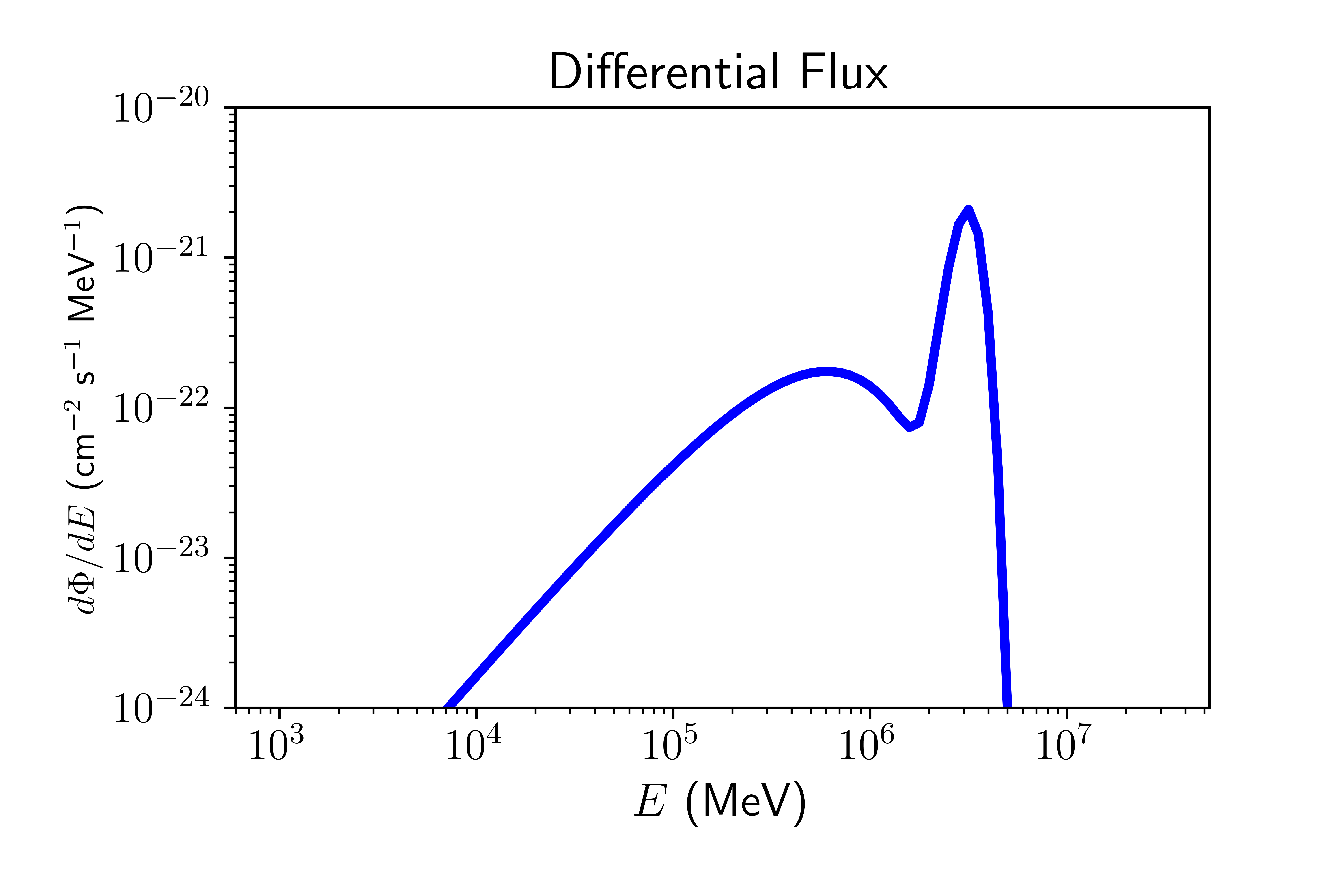
(a)

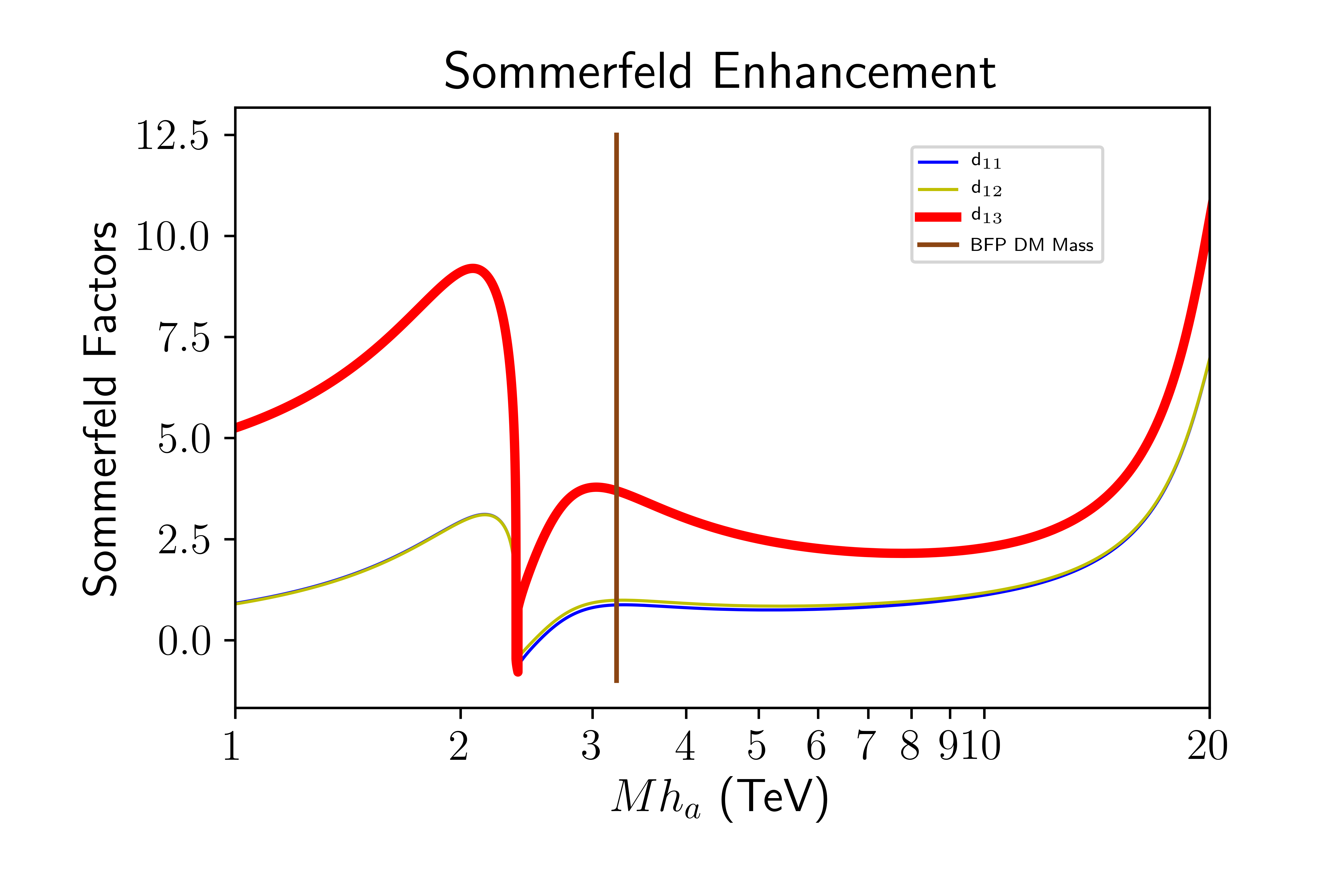
(b)

Figure 1: (a) Differential flux from DM pair annihilation (eq. 21) for the benchmark point of the model computed in section 5. (b) Sommerfeld enhancing factors as a function of the DM candidate mass, other parameters are taken as in the benchmark point. The vertical line signals the value of the benchmark DM mass.

The enhanced cross sections are then obtained with the aid of the Optical Theorem which relates the Forward Scattering Amplitude with the (tree level) annihilating amplitudes of the DM particles in the multiplet (for full details see the above references). The annihilating cross section in the limit of zero relative velocity for a given final state $f$ is given by:

$$\sigma v_{\mathrm{rel}}(h_{a}\,h_{a}\rightarrow f)=\frac{1}{2}(D\Gamma^{f}D^{\dagger})_{11}$$ (16)

where $\Gamma=\sum_{f}\Gamma^{f}$ is the total matrix of absorptive terms to all final states $f$, and $D$ is the matrix whose only nonzero row (in our basis the first row) is $d^{\mathrm{T}}$. The elements of $\Gamma^{f}$ are given explicitly by

$$\Gamma^{f}_{ij}=\frac{N_{i}N_{j}}{4M^{2}_{h_{a}}}\int\prod_{a\in f}\frac{d^{3}q_{a}}{(2\pi)^{3}2E_{a}}{\cal M}(i\rightarrow f){\cal M}^{*}(j\rightarrow f)(2\pi)^{4}\delta^{4}(p_{i}-p_{j})$$ (17)

here the indexes $i$ and $j$ refer to any element of the two-particle basis (the annihilating pair), $f$ is any allowed final state of non-DM particles in the model, $p_{i}$ and $p_{j}$ are the 4-momenta of the initial and final states and the symmetry factors are given by $N_{h_{a}h_{a}}=N_{A_{a}A_{a}}=1/\sqrt{2}$ and $N_{H_{a}^{+}H_{a}^{-}}=1$, with ${\cal M}$ the tree level corresponding annihilating amplitudes.

We compute $\Gamma^{f}$ for the following final states: $\gamma\gamma$, $\gamma Z$, $ZZ$, $W^{+}W^{-}$, $HH$, $H_{3}H_{3}$, $hh$ and $Hh$ (for $HH_{3}$ and $H_{3}h$, $\Gamma^{f}$ is zero). For example, $\Gamma^{H_{3}H_{3}}$ is given by:

$$\Gamma^{H_{3}H_{3}}=\frac{1}{32\pi M_{h_{a}}^{2}}\left(\begin{array}[]{ccc}\frac{1}{2}\lambda_{+}^{2}&\frac{9}{2}\lambda_{-}\lambda_{+}&\frac{9}{\sqrt{2}}\lambda_{10}\lambda_{+}\\ \frac{9}{2}\lambda_{-}\lambda_{+}&\frac{1}{2}\lambda_{-}^{2}&\frac{9}{\sqrt{2}}\lambda_{10}\lambda_{-}\\ \frac{9}{\sqrt{2}}\lambda_{10}\lambda_{+}&\frac{9}{\sqrt{2}}\lambda_{10}\lambda_{-}&\lambda_{10}^{2}\\ \end{array}\right)$$ (18)

where $\lambda_{\pm}\equiv\lambda_{10}+\lambda_{11}\pm 2\lambda_{12}$. Note that for this calculations we approximate the DM mass splittings as zero and we also neglect terms of the form $M_{X}/M_{h_{a}}$ with $X$ any gauge boson or scalar, for the numerical calculation we thus will keep the masses of the scalars to relatively light values. We list in appendix A the rest of the matrices.

2.3 Flux

The total differential cross section into gammas is given by

$$\frac{d\sigma v_{\mathrm{rel}}}{dE_{\gamma}}=\sum_{f}\sigma v_{\mathrm{rel}}(h_{a}h_{a}\rightarrow f)\times\frac{dN^{f}}{dE\gamma}$$ (19)

Following [29], for the case of continuous yields ($f$ = EW or scalar boson pair as final state) we use the parametrization [65]:

$$\frac{dN^{f}}{dE\gamma}=(0.73/M_{h_{a}})\,x^{1.5}\,\exp{-7.8\,x}$$ (20)

with $x=E\gamma/M_{h_{a}}$. For the $\gamma\gamma$ or the $\gamma Z$ final states the yield is a Dirac delta centered respectively at $M_{h_{a}}$ or $M_{h_{a}}-M_{Z}^{2}/(4M_{h_{a}})$. We model the delta as a Gaussian centered at the corresponding energy and of width equal to (conservatively) 15% the energy of the line, this since a delta would be a “monochromatic line” which in the context of ID experiments refers to spectral features with energy width much smaller than the energy resolution of the detector, typically 15% is achieved e.g. in HESS and therefore such value would be conservative for the CTA. Thus, with Gaussian width = 0.15 $M_{h_{a}}$: $(dN/dE\gamma)^{\gamma\gamma}=2\delta(E_{\gamma}-M_{h_{a}})=2(2.66/M_{h_{a}})\exp(-22.22(x-M_{h_{a}})^{2}/M_{h_{a}}^{2})$ and similar for $\gamma Z$.

Finally, the predicted gamma ray flux from annihilation of DM particles is given by the expression:

$$\frac{d\Phi_{\gamma}}{dE_{\gamma}}=\frac{1}{4\pi}\left(\int_{\Delta\Omega}d\Omega\int_{l.o.s}ds\rho^{2}_{\chi}\right)\left[\frac{1}{2M_{h_{a}}^{2}}\sum_{f}\sigma v_{\mathrm{rel}}(h_{a}h_{a}\rightarrow f)\frac{dN^{f}}{dE_{\gamma}}\right]$$ (21)

here we have deliberately separated the equation into two parts, since the computation involved for each part is of very different nature. The first part (the astrophysical part) is well establish for example in the case of dwarf spheroidal galaxies from astrophysical observations and it is known as the “J-factor”, we will take the dwarf as a point source with constant J-factor of $\log_{10}J=19.52$ (with $J$ in GeV² cm^-5) [66]. With the analysis of the previous section and the expressions for the yields given above we complete the second part and the flux prediction from the model.

3 Likelihood estimate

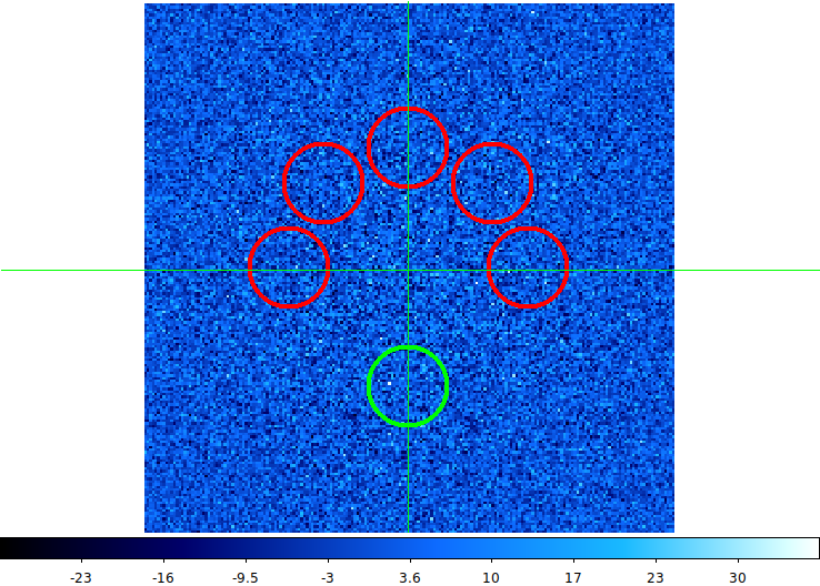
Figure 2: On and Off-regions for the observation of the Coma Berenices spherical dwarf and the determination of the background. The dwarf is located in the center of the green circle at the bottom, and five adjacent regions (red circles) located in symmetric points with respect to the observation point are use to determine the background signal, the telescope aim is located at the center of the intersecting lines. The color axis represents the signal detection significance, the absence of notorious bright spots in the region means that no known sources of gamma rays need to be taken into account in the determination of the background.

We choose to make our analysis based on a simulation of future observations of the dwarf spheroidal (dSph) galaxy Coma Berenices (or Coma) by the Cherenkov Telescope Array (southern hemisphere branch). Coma Berenices was discovered in 2006 by the Sloan Digital Sky Survey [67] and is a faint Milky Way satellite at a distance of 44 kpc from the Sun with right ascension of 12 h 26 min 59 sec and declination of 23 deg 54 min 15 sec; it is estimated to have a $J$-factor of $\log_{10}J=19.52$, $J$ in GeV² cm^-5 [66]. dSph galaxies are recurrent targets for searches of DM signals in ID experiments by virtue of their large inferred DM density and no known natural sources of gamma rays, Coma for example was part of a recent study of several dSphs in a DM signal search from HESS [68]; here, we try to follow their general analysis strategy in as much as possible as the available public tools allow us.

We simulate an observation run of Coma of 20 hours with the southern hemisphere CTA array in which we further assume a no-result experiment, in other words we assume that no significant excess of gamma rays above nominal background is found throughout the observation period. This will allow us to predict, based on current estimations of CTA’s expected baseline performance, exclusion limits on the parameter space of this particular model. We perform our analysis employing the reflected background technique [69] where the position of the telescope aim is slightly offset from the objective, the latter defined as a circular region (the On region) centered around Coma from which the simulated observation is used to fit against the predicted flux from the model. To compute the background in this technique several twin regions (the Off regions) are defined in symmetrical positions around the telescope aim (see figure 2) from which the background rate is extracted from the public Instrument Response Function (IRF) provided by the CTA Consortium. Background rates are expected to be fairly symmetric with respect to the position of the camera aim and thus this method minimizes a possible source of systematic errors from modeling the background from Monte Carlo simulations.

In an On/Off analysis the model $M$ is composed of the signal (predicted number of gamma rays) and the background $M=M_{s}+M_{b}$, the background model $M_{b}$ is taken from the background information provided in the IRF and the signal $M_{s}$ is calculated from the predicted differential gamma ray flux. The likelihood estimate is constructed from the formula:

$$-\log{\cal L}(M)=\sum_{i}{s_{i}(M_{s})+a_{i}(M_{b})b_{i}(M_{b})-n_{i}^{\mathrm{on}}\log[s_{i}(M_{s})+a_{i}(M_{b})b_{i}(M_{b})]+b_{i}(M_{b})-n_{i}^{\mathrm{off}}\log{b_{i}(M_{b})}}$$ (22)

where $n_{i}^{\mathrm{on}}$ ($n_{i}^{\mathrm{off}}$) is the number of events in bin $i$ of the On (Off) region, $s_{i}(M_{s})$ ($b_{i}(M_{b})$) is the number of expected signal (background) counts in bin $i$ of the On (Off) region and $a_{i}(M_{b})$ is the ratio between the spatial integral over the background model in the On region and the Off region for bin $i$.

The detection significance of the model is estimated using the Test Statistic (TS) which is defined as:

$$\mathrm{TS}=2[\log{{\cal L}(M_{s}+M_{b})}-\log{{\cal L}(M_{b})}]$$ (23)

which involves the log-likelihood value obtained when fitting the model and the background together to the simulated data, and also the log-likelihood value when fitting only the background.

Note that for the calculation of this quantities all the parameters of the theoretical model remain fixed because the construction of the likelihood profile is done by an external (to the CTA tools) minimizer which in each step provides a set of model parameter values along with the predicted differential flux, requests the value of the CTA likelihood function (from the CTA tools), computes additional likelihood components and based on this information moves around in parameter space searching for the maximum of the total likelihood function, as explained in the next section.

4 Numerical analysis

The setup for the numerical computation is very simple, we define a function $F$ which accepts as input a set of values for the free parameters of the model and returns the value of the total likelihood function. The problem is then reduced to the maximization of this function, for this we use Diver [70] in standalone mode, the differential evolution scanner available in the Gambit [71] package, and for post-processing of the resulting data sets we use Pippi [72]. To reduce the number of free parameters of the model in the scan we fix the value of the scalar $h$ to the Higgs mass [73, 74], for simplicity we fix $\lambda_{13}=0.001$ to easily satisfy inequalities that ensure no tunneling to vacua that breaks the $Z_{2}$ discrete symmetry [20], and we take $\mu_{2}^{2}$ given in terms of the DM mass ($M_{h_{a}}^{2}-\mu_{2}^{2}$ small constant) so that the gaps $M_{H_{a}^{\pm}}-M_{h_{a}}$ and $M_{A_{a}}-M_{h_{a}}$ can be taken relatively small in order to explore regions that presumably have big enhancement factors of the annihilation cross section. For the same reason, we take the masses of the heavy scalars in-between 200 and 800 GeV, since the larger the masses of these particles the minor the contribution to the deforming potential in the Sommerfeld factor.

The layout of $F$ is a little bit more technically challenging though. Basically we divide points of the model’s parameter space into two categories, the ones that satiate the physical constraints and the ones that doesn’t. In the latter case we don’t discard the points, instead equivalently, we assign a bad likelihood to them. Construction of the constraint filters is done with the aid of several public tools: we implement the model in SARAH [75, 76, 77, 78] from which we generate corresponding model files for the rest of the tools. Tree level LQT [79] and finite energy [80] unitarity conditions are calculated with the SARAH-SPheno [81, 82, 83] framework, and we check current experimental limits from Higgs and heavy scalar searches using HiggsBounds [84, 85, 86, 87, 88]. For a more complete description of the implementation of the constraints see our previous work [53].

Next we compute the Sommerfeld factors (15) by solving the corresponding coupled equations (13) by means of a fourth-order Rosenbrock method [89], the non-relativistic potentials, scattering and annihilation amplitudes are obtained with the aid of FeynArts [90], FormCalc [91] and FeynCalc [92, 93, 94]. This allow us to calculate the enhanced annihilation cross sections from which we compute the differential gamma ray flux using (21).

From the predicted differential flux a file with energy and differential flux columns is created which is then fed to ctools [95, 96], the public software package for the scientific analysis of Cherenkov Telescope Array data and simulations. With the aid of ctools, an On/Off analysis of the model is performed along the lines described in the previous section deriving one piece of the likelihood value up to this point. We treat Coma as a point-like source and the size of the on and off regions are taken to be 0.3 degrees in radius. We note that this part of the calculation is the most expensive in terms of computational time, with so much free parameters and taking into account that a total of approximately $4.5\times 10^{7}$ $F$-function evaluations are needed for the algorithm to converge and find the absolute maximum of the likelihood function, this makes the inclusion of more than one dwarf in the analysis unpractical with the computational resources at hand, because the position of the dwarfs in the sky are very different and an independent analysis for each one of them has to be done and therefore the time expended in each dwarf would be the same, increasing linearly the total time of the run.

Finally the computation of the value of the relic abundance is made with the aid of MicrOMEGAS [97]. To allow for the possibility of under-abundant DM candidate we penalize only relic abundance values above the Planck experimental measured interval [98], points with a value of this observable conforming to or below the Planck value are assigned a likelihood value of $1/(\sqrt{2\pi}\sigma)$ with $\sigma$ the Planck measured interval, this likelihood value is added to the previously calculated one.

More technical details of the procedure described here can be found in the source codes of the modules used to generate the results of this research, see [99].

Figure 3: Spectrum of masses of the scalar particles in the model evaluated at the BFP.

5 Results

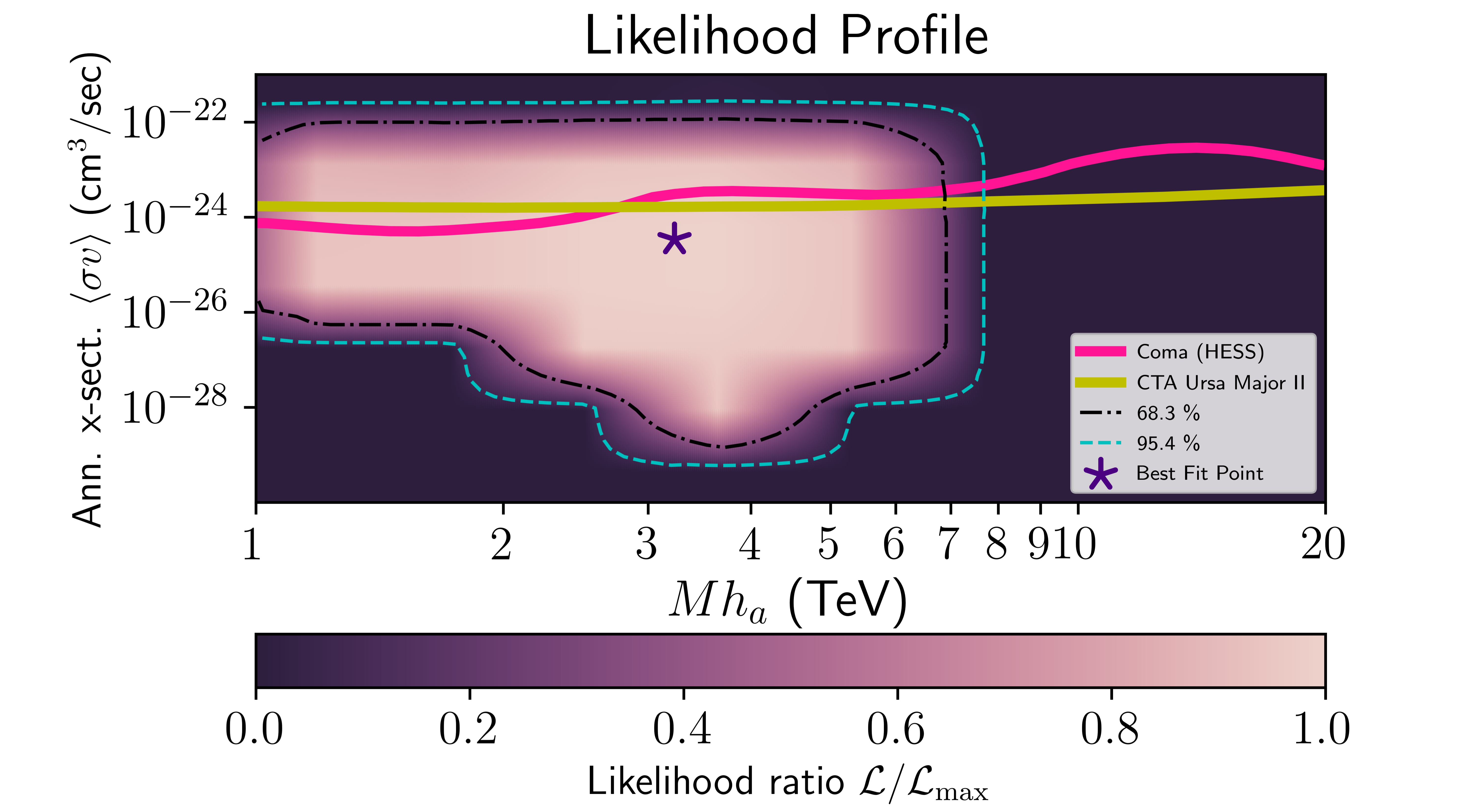
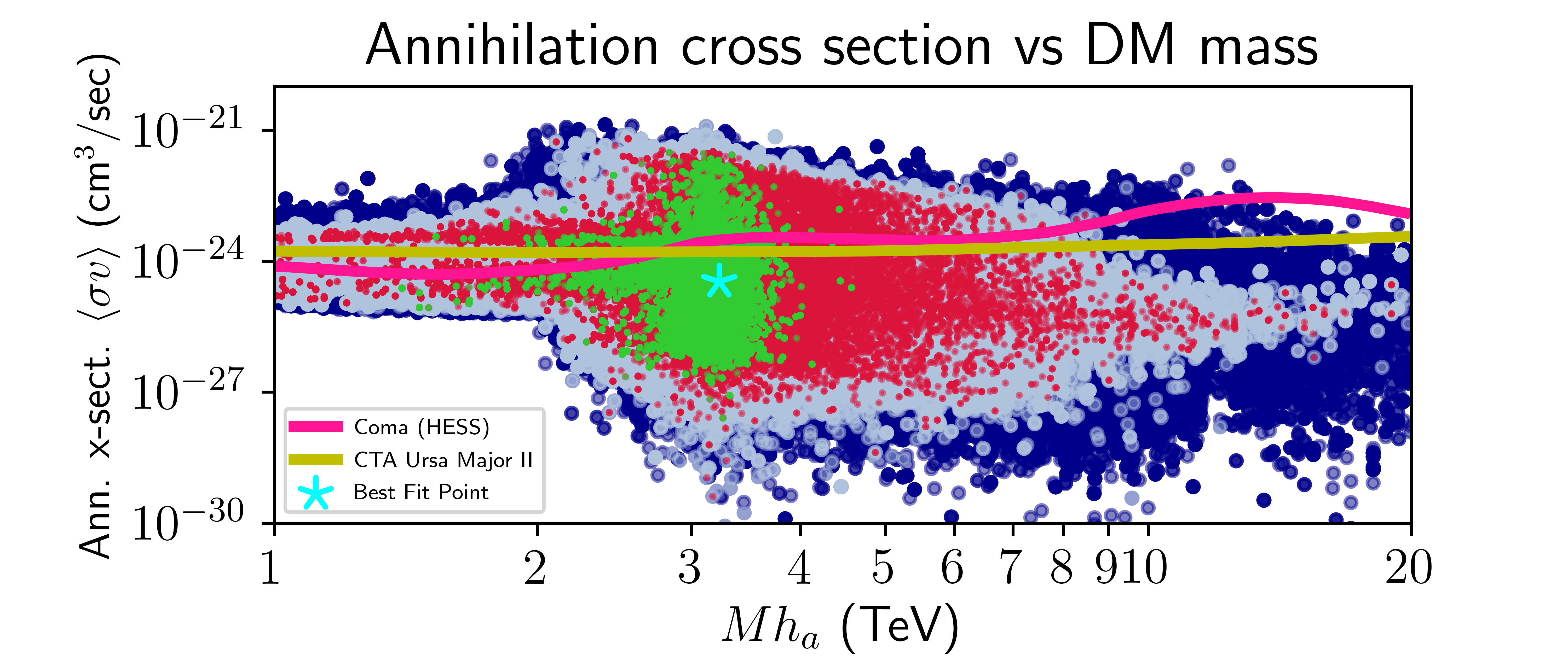
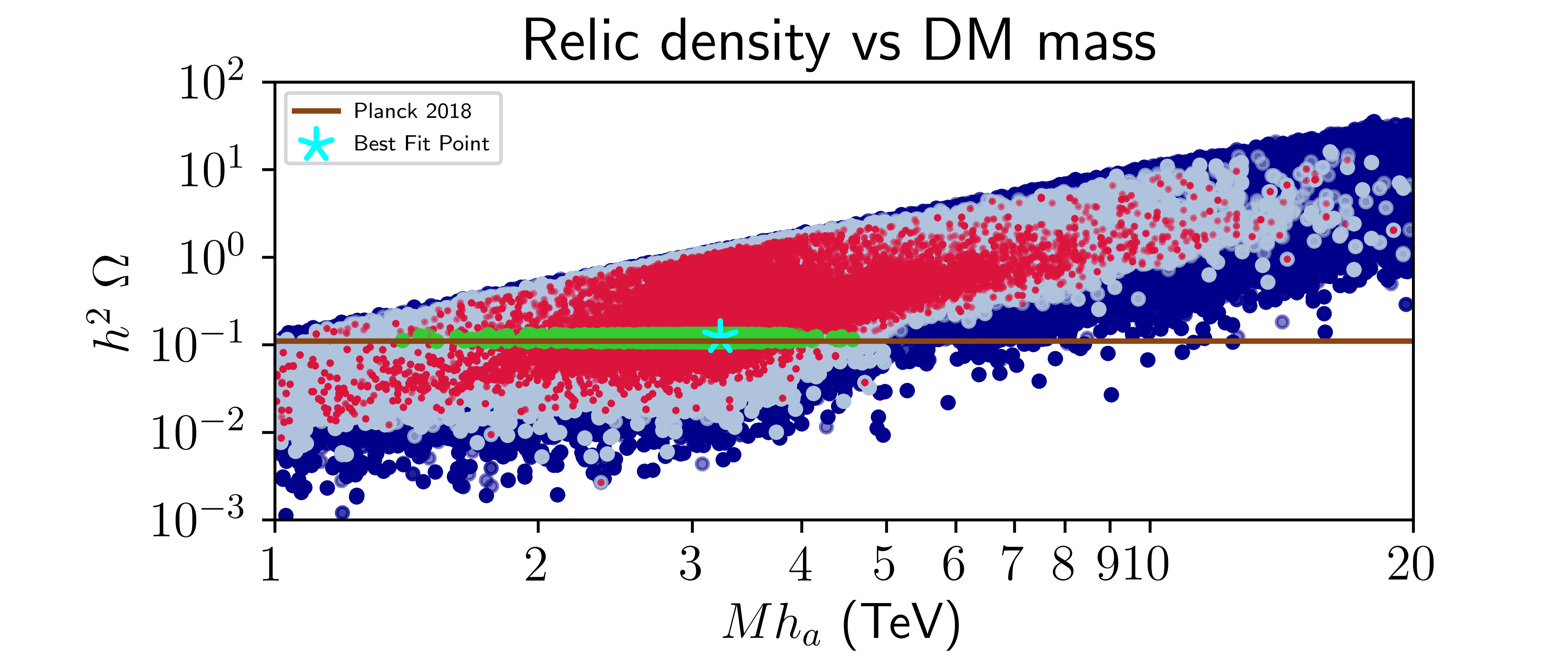
Figure 4: (Color online) Top panel: Normalized likelihood profile as a function of the zero-velocity averaged annihilation cross section and the DM candidate mass. Contours for a coverage probability of 68.3% and 95.4% for two degrees of freedom are shown as dot dashed and dashed respectively, and the BFP is marked as a star. For comparison we show exclusion curves from an analysis of an observation of Coma by HESS [68] and a simulation of a CTA observation of Ursa Major II [100] (both model independent analysis). Middle panel: Scatter plot of the annihilation cross section as a function of the DM mass, navy blue points are consistent with unitarity and stability bounds but are excluded from experimental scalar searches; light blue points are consistent with all of these constraints while the red points in addition satisfy the decoupling limit for $h$; green points predict a relic abundance within the experimental Planck value [98]. Bottom panel: Scatter plot of the predicted relic abundance as a function of the DM mass, the color code of the points is the same as the middle panel.

We report here our results obtained from a final run with a population of 40 thousand points for the minimizer. The spectrum of masses of the scalar sector at the best fit point is presented in figure 3, the DM sector masses are intentionally kept quasi-degenerate in order to facilitate the occurrence of the Sommerfeld effect by allowing the production of on-shell DM intermediate states other than $h_{a}$ (by keeping the DM mass gaps small), we find that the heavy (non DM) scalars lie with masses in between 278 and 509 GeV.

In figure 4 bottom panel, we present a scatter plot of points in the parameter space of the model and their predictions of the value of the relic abundance as a function of the mass of the DM candidate, the points are color coded according to weather or not they satisfy all physical constraints. With navy blue points excluded from heavy scalar experimental searches, the rest of the points satisfy this constraint as well as unitarity and stability and thus this plot makes it clear that only the region below the Planck value (the horizontal line) represents physically acceptable points (assuming also the possibility of an under-abundant DM candidate). Therefore, the region with DM masses above $\sim$5 TeV is clearly excluded. The difference between the light blue points and the red ones is that for the latter the scalar $h$ is within the decoupling limit and thus has all the characteristics of the SM Higgs particle. In addition, green points (a subset of the red ones) predict a relic abundance within the experimental Planck interval, note that we found this kind of points within a region approximately from $\sim$1.3 to $\sim$4.9 TeV masses.

In the middle panel of figure 4 we present a scatter plot of the annihilation cross section versus the DM candidate mass with the same color code for the points as above. We include in the plot two exclusion curves from independent analysis. The first, labeled Coma (HESS), is an analysis of the Coma Dwarf from observations with the HESS Imaging Atmospheric Cherenkov Telescopes [68] and represents a 95% C.L. exclusion limit on the velocity weighted cross section for DM self-annihilation into gamma ray lines ($\gamma\gamma$ lines). They also include combined analysis with other dwarfs but we chose to present the comparison only with the limits from the observations of Coma Berenices; note that this limits assume generic DM (or model independent). The second exclusion curve, labeled CTA Ursa Major II, is from a simulation of the CTA sensitivity to DM annihilation in the channel DM DM $\rightarrow W^{+}W^{-}$ assuming a 500 hour observation of the Ursa Major II dwarf [100], also for generic dark matter; while in this reference there are also limits from Coma Berenices (but only 50 hour observation simulation), we chose to compare with Ursa Major II because it has more stringent limits. We note from this scatter plot that there is a “depression” starting around masses of 2 TeV where the cross section begins to take smaller values, this may be indicative that the destructive interference in the enhancement factors found in the BFP (figure 1) in between 2 and 3 TeV values of the DM mass is a generic feature of the parameter space and not only of the BFP.

Next, in the top panel of figure 4 we present the normalized likelihood profile as a function of the annihilation cross section and the DM candidate mass, the best fit point of the analysis is marked as a star (in all panels); we note how the region above a DM mass of 5 TeV is gradually disfavored mostly because it is already ruled out by an overproduction of DM not consistent with observations. It is apparent from this plot that close to a third of the viable region of plausible physical points lie above the two exclusion curves which are very similar in the region of masses below 7 TeV, with the HESS limits slightly better below $\sim$3 TeV and the CTA limits slightly better above this mass. Both exclusion curves come very close to disfavour the best fit point of the model, probably with an improvement of the limits by an order of magnitude the BFP could be excluded. Notice that we are assuming the possibility of under-abundant DM, had we imposed penalization of the likelihood function also for points below the Planck interval by the assumption that this DM candidate comprises the totality of the observed DM in the Universe, then the bright region of this plot would appear shrunken horizontally reflecting the fact that green points in the other plots lie mostly around a mass of $\sim$3.1 TeV, as noted before.

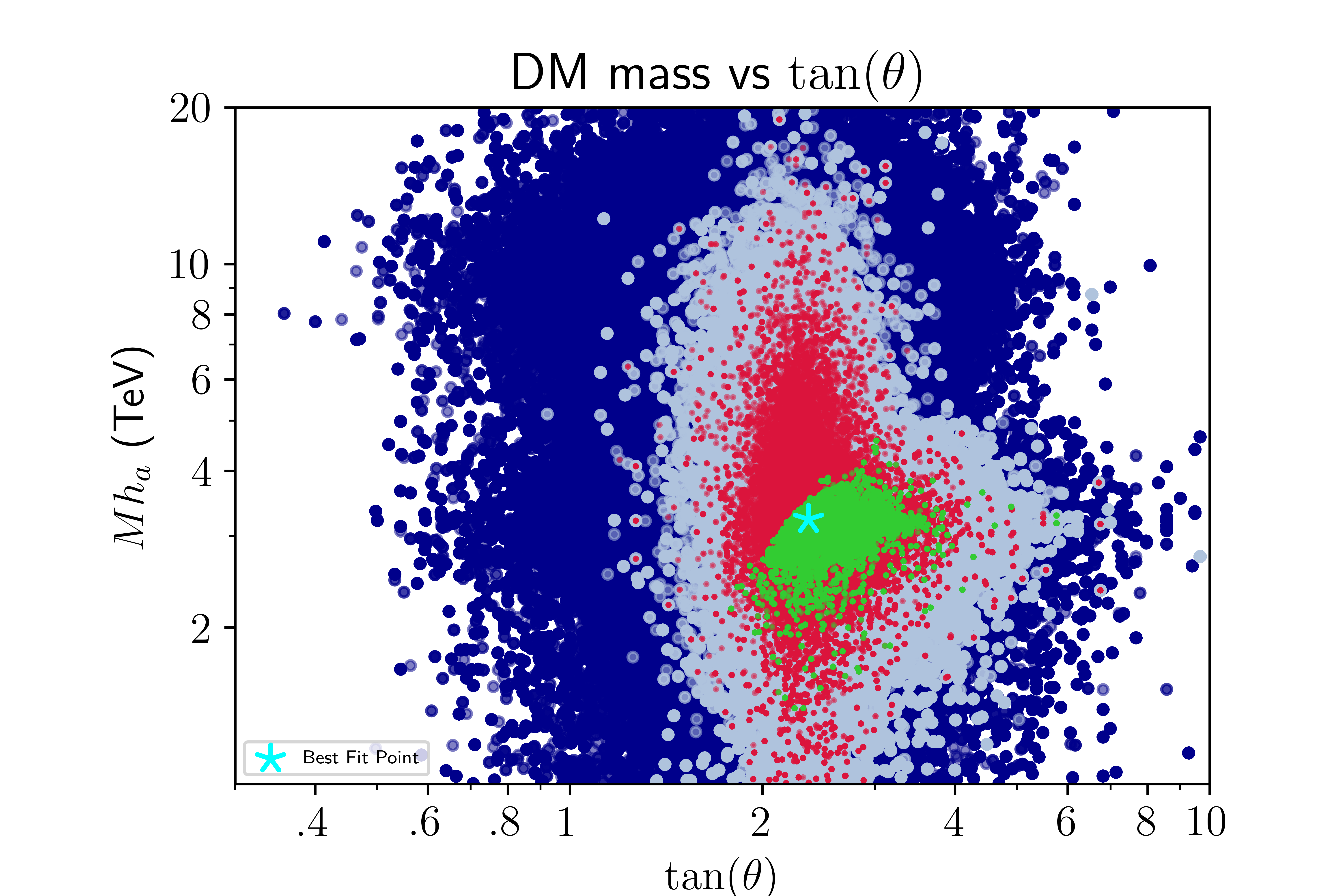
Figure 5: (Color online) Scatter plot of the DM mass as a function of $\tan\theta$, the color code of the points is as in figure 4.

In figure 5 we show an scatter plot of the DM mass candidate as a function of $\tan\theta$ with the color coding the same as in the previous scatter plots. We see clearly the approximately formation of subregions contained within regions of a lesser restraining level, thus points that satisfy the decoupling limit cover around two thirds of the region of points satisfying unitariry, stability and Higgs searches, while points predicting a relic abundance value within the experimental interval lie mostly between values of $\tan\theta$ equal 2 and 4, with the BFP attaining a value of 2.34.

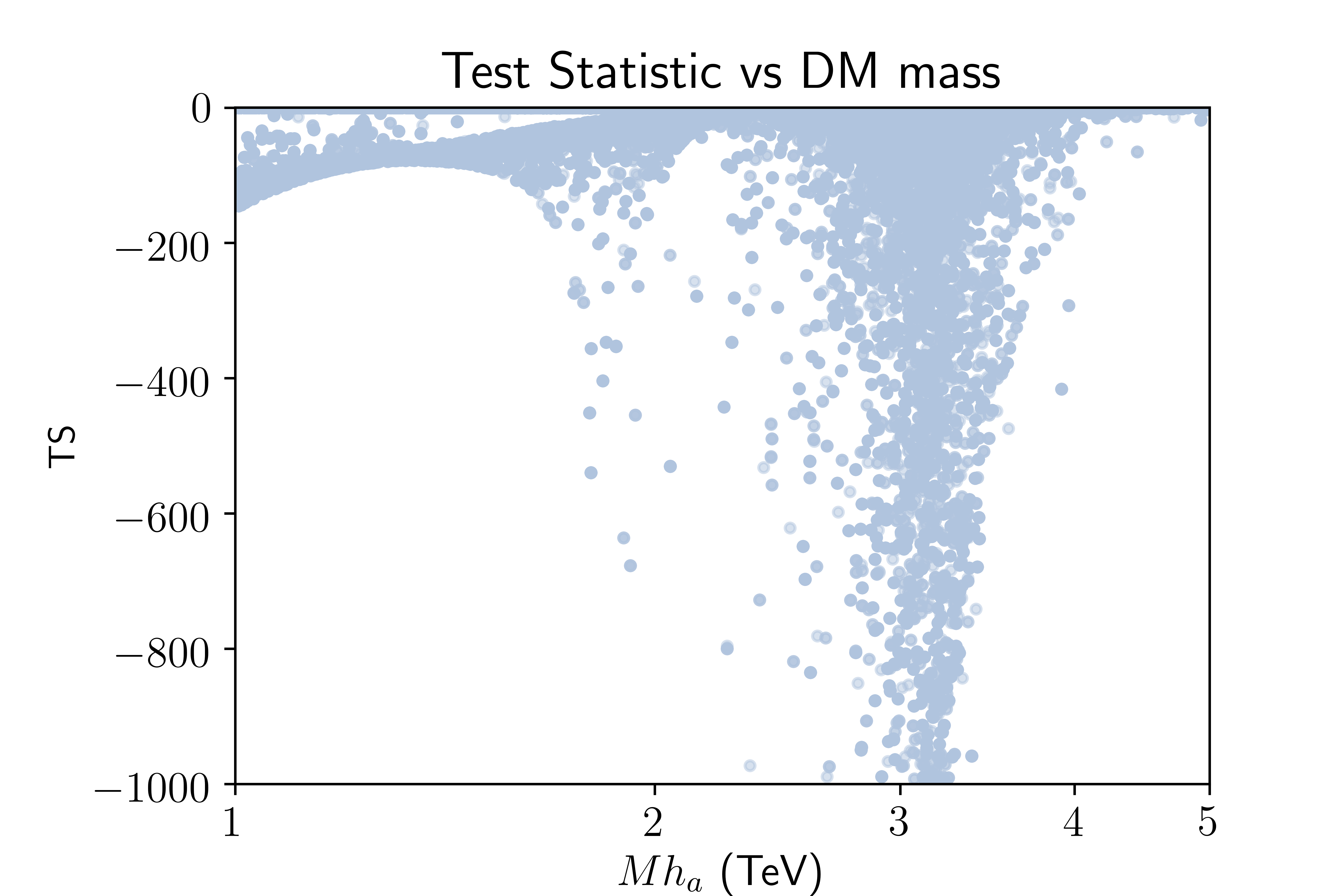
(a)

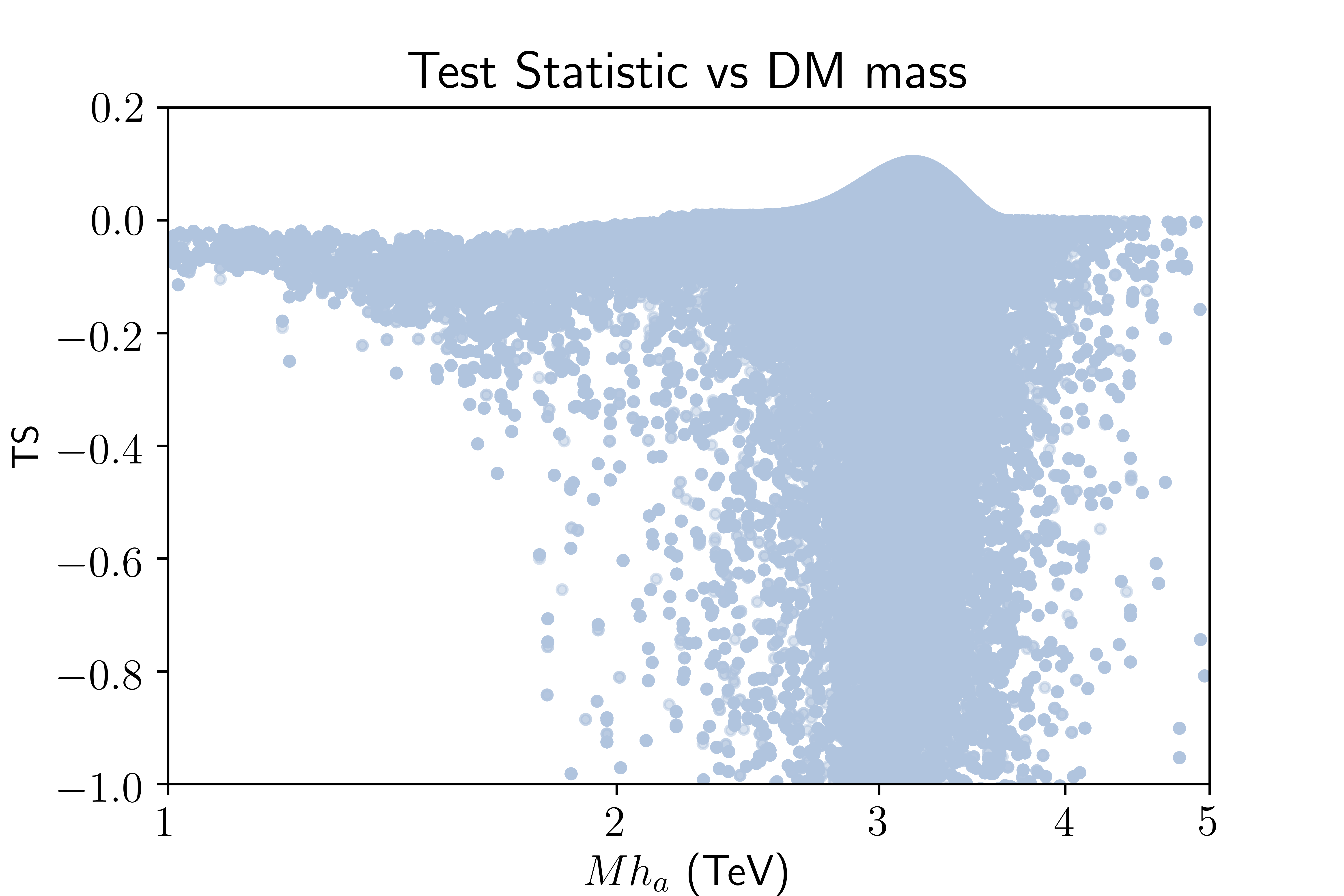
(b)

Figure 6: (a) Scatter plot of the Test Statistic as a function of the DM mass, all the points shown satisfy unitarity, stability and experimental higgs searches constraints and in addition predict a relic abundance within the experimental Planck value or below it. (b) Same as (a) but shows only values above a TS > -1.0.

Since we are simulating a null-result experiment, the best indicator of the actual sensibility of the experiment would be the computation of the Test Statistic to compare to what is expected under the null hypothesis (no DM present), this technique is employed in current ID experiments to construct exclusion limits from their non-observation of significant gamma ray signals above the background. With this in mind, we present in figure 6 (a) the scatter plot of the TS as a function of the DM mass in the DM mass range between 1 and 5 TeV, this accounting for the fact that higher masses predict overproduction of DM in conflict with the observed abundance as was discussed before. In fact, during the computational runs the calculation of the CTA likelihood and the TS was not performed for points predicting a relic above the Planck interval. Instead, these points were automatically assigned a “bad” value of the likelihood for purposes of optimization of the code. Figure 6 (b) shows the same plot but only for TS > -1.0, here we note that the TS reaches an almost constant maximum value very close to zero for a given mass, with a small bulb around a DM mass of $\sim$3.2 TeV, attaining a maximum TS close to 0.1.

For points in figure 6 lying in a (vertical) ray of constant DM mass, we consider the difference $TS_{\textrm{max}}-TS\equiv\Delta TS$, since the Test Statistic approaches a $\chi^{2}$ function in the large data sample limit, a value of $\Delta TS=1$ corresponds to a coverage probability of 68.3% for estimation of 1 parameter [101], which we take as the annihilation cross section. Therefore, we interpret points in such a ray with $\Delta TS>1$ as excluded with a C.L. of 68%. In this manner we construct a “Test Statistic profile”, shown in figure 7 as a function of the annihilation cross section and the DM mass. Since the value of $TS_{\textrm{max}}$ is very small, for points such that $\Delta TS\gtrsim 1$ we approximate $\Delta TS\approx|TS|$ and the limit condition becomes $|TS|>1$ for them. Following these arguments, we consider the points in the upper region of this figure excluded by our analysis (at the corresponding C.L.) while the points in the bottom region are not. We can then interpret the boundary of the upper (green) region as an approximate exclusion curve, except that there is an overlapping of the two regions, which we take as a consequence of the error bars of the analysis, though a precise determination of these errors will not be pursued here.

6 Conclusions

We have presented in this letter an analysis of the Dark $S3$ model in the region of high dark matter candidate mass pursuing a determination of the prospects of indirect detection specific to this model. In order to take into account most of the important theoretical predictions of the model we calculated the non-relativistic potentials which potentially can cause enhancements on the value of the annihilation cross section by means of the Sommerfeld effect. We computed the enhancement factors and the annihilation matrices leading to a proper determination of the cross sections and the differential gamma ray flux from annihilation of DM pairs in the Coma Berenices dwarf galaxy. We determined then the likelihood profile in parameter space from a simulation of observations of such dwarf galaxy at the CTA assuming a null-result experiment using available public tools. We conclude from our results that DM masses above 5 TeV are definitely exclude mainly because of overproduction of DM not consistent with the observed value of the relic abundance. For masses below 5 TeV the best fit point of the likelihood analysis suggest a DM value of $\sim$ 3.14 TeV, somewhat higher than the value where the highest cross section enhancement occurs indicating that other constraints such as unitarity and scalar searches are also important for the precise determination of the best fit. Comparison of our results with independent analysis in the literature shows that current as well as estimated exclusion limits are close to disfavour the model’s BFP, at least under the conditions of the present analysis. Perhaps the inclusion of a combined analysis taking into consideration several more dwarf galaxies will allow more stringent limits on the model.

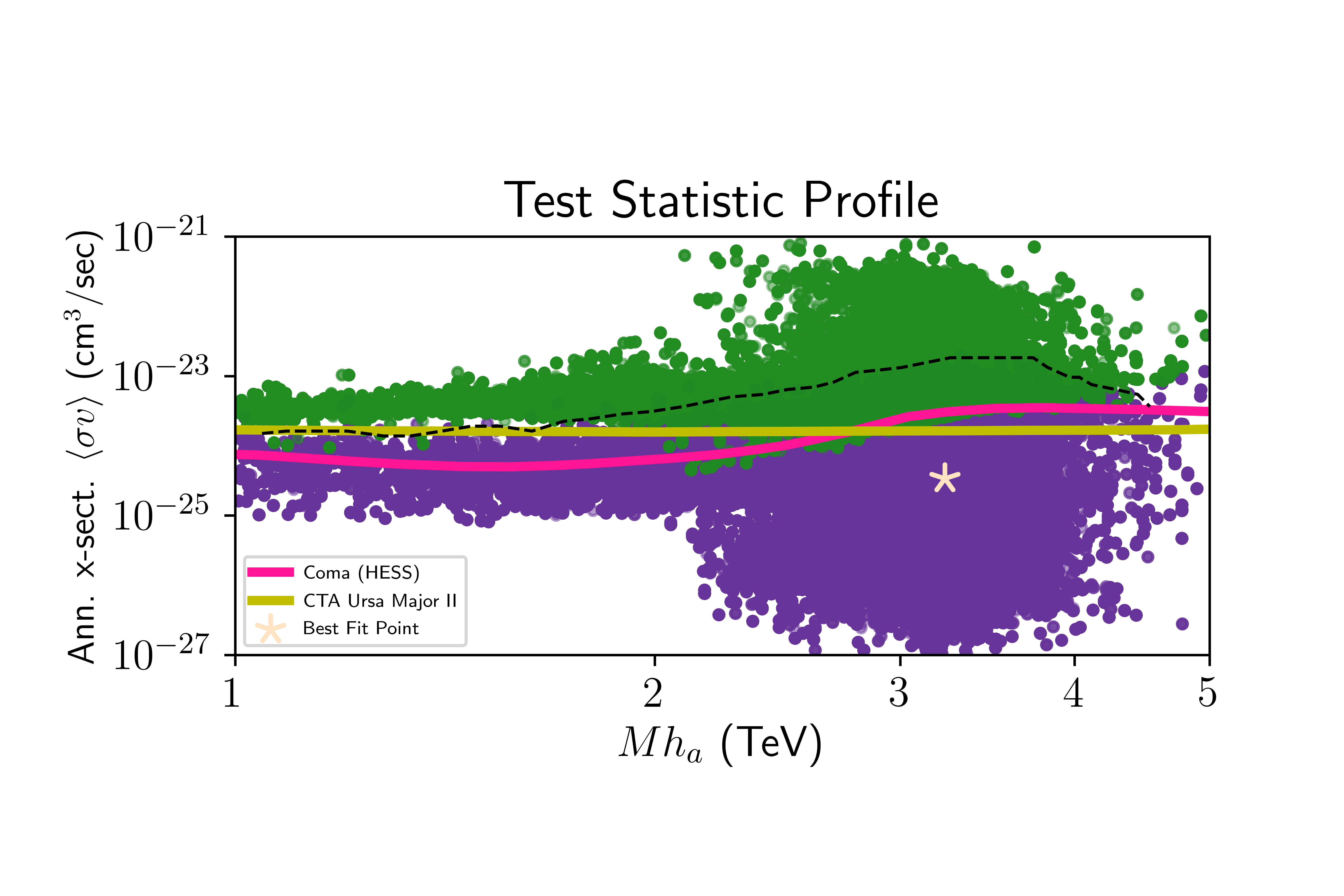
Figure 7: (Color online) Scatter plot of the annihilation cross section as a function of the DM mass with the points colored according to their value of the Test Statistic: purple points (mostly bottom region) have a TS less than 1 in absolute value, while green points (mostly top region) have a TS greater than 1 in absolute value. The exclusion curves are as in figure 4 and the dashed black line shows the extend to which the purple and the green points overlap (for more details see main text).

Appendix A Absorptive terms

In this appendix we list the non-zero (symmetric) matrices of absorptive terms for the calculation of the enhanced annihilation DM cross section that complement equation (18).

Channel $\gamma\gamma$:

$$\Gamma^{\gamma\gamma}=\frac{e^{4}}{4\pi M_{h_{a}}^{2}}\times\mathrm{diag}(0,0,1)$$ (24)

Channel $\gamma Z$:

$$\Gamma^{\gamma Z}=\frac{e^{4}\cot^{2}(2\theta_{w})}{4\pi M_{h_{a}}^{2}}\times\mathrm{diag}(0,0,1)$$ (25)

Channel $ZZ$:

$$\begin{array}[]{l@{}l}\Gamma^{ZZ}_{11}&{}=\frac{1}{1024\pi M_{h_{a}}^{2}}(8g_{2}^{4}\sec^{4}(\theta_{w})+4(-\cos(2\theta)(\lambda_{+}-\lambda_{14})+\lambda_{+}+\lambda_{14})^{2})\\ \Gamma^{ZZ}_{12}&{}=\frac{1}{512\pi M_{h_{a}}^{2}}(4g_{2}^{4}\sec^{4}(\theta_{w})-4\cos(2\theta)\left((\lambda_{10}+\lambda_{11})^{2}-4\lambda_{12}^{2}-\lambda_{14}^{2}\right)+\cos(4\theta)(\lambda_{+}-\lambda_{14})(\lambda_{-}-\lambda_{14})\\ &{}+2\lambda_{14}(\lambda_{10}+\lambda_{11})+3(\lambda_{10}+\lambda_{11})^{2}-12\lambda_{12}^{2}+3\lambda_{14}^{2})\\ \Gamma^{ZZ}_{13}&{}=\frac{1}{64\sqrt{2}\pi M_{h_{a}}^{2}}(g_{2}^{4}\cos^{2}(2\theta_{w})\sec^{4}(\theta_{w})+\lambda_{10}\sin^{2}(\theta)(-\cos(2\theta)(\lambda_{+}-\lambda_{14})+\lambda_{+}+\lambda_{14}))\\ \Gamma^{ZZ}_{22}&{}=\frac{1}{1024\pi M_{h_{a}}^{2}}(8g_{2}^{4}\sec^{4}(\theta_{w})+4(-\cos(2\theta)(\lambda_{-}-\lambda_{14})+\lambda_{-}+\lambda_{14})^{2})\\ \Gamma^{ZZ}_{23}&{}=\frac{1}{64\sqrt{2}\pi M_{h_{a}}^{2}}(g_{2}^{4}\cos^{2}(2\theta_{w})\sec^{4}(\theta_{w})+\lambda_{10}\sin^{2}(\theta)(-\cos(2\theta)(\lambda_{-}-\lambda_{14})+\lambda_{-}+\lambda_{14}))\\ \Gamma^{ZZ}_{33}&{}=\frac{1}{64\pi M_{h_{a}}^{2}}(g_{2}^{4}\cos^{4}(2\theta_{w})\sec^{4}(\theta_{w})+2\lambda_{10}^{2}\sin^{4}(\theta))\end{array}$$ (26)

Channel $W^{+}W^{-}$:

$$\begin{array}[]{l@{}l}\Gamma^{W^{+}W^{-}}_{11}&{}=\frac{1}{512\pi M_{h_{a}}^{2}}(4g_{2}^{4}-4\cos(2\theta)(\lambda_{+}-\lambda_{14})(\lambda_{+}+\lambda_{14})+\cos(4\theta)(\lambda_{+}-\lambda_{14})^{2}\\ &{}+2\lambda_{14}(\lambda_{+})+3(\lambda_{+})^{2}+3\lambda_{14}^{2})\\ \Gamma^{W^{+}W^{-}}_{12}&{}=\frac{1}{512\pi M_{h_{a}}^{2}}(4g_{2}^{4}-4\cos(2\theta)\left((\lambda_{10}+\lambda_{11})^{2}-4\lambda_{12}^{2}-\lambda_{14}^{2}\right)+\cos(4\theta)(\lambda_{+}-\lambda_{14})(\lambda_{-}-\lambda_{14})\\ &{}+2\lambda_{14}(\lambda_{10}+\lambda_{11})+3(\lambda_{10}+\lambda_{11})^{2}-12\lambda_{12}^{2}+3\lambda_{14}^{2})\\ \Gamma^{W^{+}W^{-}}_{13}&{}=\frac{1}{256\sqrt{2}\pi M_{h_{a}}^{2}}(4g_{2}^{4}+\lambda_{10}\cos(4\theta)(\lambda_{+}-\lambda_{14})+\lambda_{10}(3(\lambda_{+})+\lambda_{14})-4\lambda_{10}\cos(2\theta)\lambda_{+})\\ \Gamma^{W^{+}W^{-}}_{22}&{}=\frac{1}{512\pi M_{h_{a}}^{2}}(4g_{2}^{4}-4\cos(2\theta)(\lambda_{-}-\lambda_{14})(\lambda_{-}+\lambda_{14})+\cos(4\theta)(\lambda_{-}-\lambda_{14})^{2}+2\lambda_{14}(\lambda_{-})\\ &{}+3(\lambda_{-})^{2}+3\lambda_{14}^{2})\\ \Gamma^{W^{+}W^{-}}_{23}&{}=\frac{1}{256\sqrt{2}\pi M_{h_{a}}^{2}}(4g_{2}^{4}+\lambda_{10}\cos(4\theta)(\lambda_{-}-\lambda_{14})+\lambda_{10}(3(\lambda_{-})+\lambda_{14})-4\lambda_{10}\cos(2\theta)(\lambda_{-}))\\ \Gamma^{W^{+}W^{-}}_{33}&{}=\frac{1}{256\pi M_{h_{a}}^{2}}(4g_{2}^{4}+\lambda_{10}^{2}(\cos(4\theta)-4\cos(2\theta))+3\lambda_{10}^{2})\\ \end{array}$$ (27)

Channel $HH$:

$$\begin{array}[]{l@{}l}\Gamma^{HH}_{11}&{}=\frac{1}{64\pi M_{h_{a}}^{2}}(\left(\sin^{2}(\alpha)(\lambda_{+})+\lambda_{14}\cos^{2}(\alpha)\right)^{2})\\ \Gamma^{HH}_{12}&{}=\frac{1}{64\pi M_{h_{a}}^{2}}(9\left(\sin^{2}(\alpha)(\lambda_{-})+\lambda_{14}\cos^{2}(\alpha)\right)\left(\sin^{2}(\alpha)(\lambda_{+})+\lambda_{14}\cos^{2}(\alpha)\right))\\ \Gamma^{HH}_{13}&{}=\frac{1}{32\sqrt{2}\pi M_{h_{a}}^{2}}(9\lambda_{10}\sin^{2}(\alpha)\left(\sin^{2}(\alpha)(\lambda_{+})+\lambda_{14}\cos^{2}(\alpha)\right))\\ \Gamma^{HH}_{22}&{}=\frac{1}{64\pi M_{h_{a}}^{2}}(\left(\sin^{2}(\alpha)(\lambda_{-})+\lambda_{14}\cos^{2}(\alpha)\right)^{2})\\ \Gamma^{HH}_{23}&{}=\frac{1}{32\sqrt{2}\pi M_{h_{a}}^{2}}(9\lambda_{10}\sin^{2}(\alpha)\left(\sin^{2}(\alpha)(\lambda_{-})+\lambda_{14}\cos^{2}(\alpha)\right))\\ \Gamma^{HH}_{33}&{}=\frac{1}{32\pi M_{h_{a}}^{2}}(\lambda_{10}^{2}\sin^{4}(\alpha))\\ \end{array}$$ (28)

Channel $hh$:

$$\begin{array}[]{l@{}l}\Gamma^{hh}_{11}&{}=\frac{1}{64\pi M_{h_{a}}^{2}}(\left(\cos^{2}(\alpha)(\lambda_{+})+\lambda_{14}\sin^{2}(\alpha)\right)^{2})\\ \Gamma^{hh}_{12}&{}=\frac{1}{64\pi M_{h_{a}}^{2}}(9\left(\cos^{2}(\alpha)(\lambda_{-})+\lambda_{14}\sin^{2}(\alpha)\right)\left(\cos^{2}(\alpha)(\lambda_{+})+\lambda_{14}\sin^{2}(\alpha)\right))\\ \Gamma^{hh}_{13}&{}=\frac{1}{32\sqrt{2}\pi M_{h_{a}}^{2}}(9\lambda_{10}\cos^{2}(\alpha)\left(\cos^{2}(\alpha)(\lambda_{+})+\lambda_{14}\sin^{2}(\alpha)\right))\\ \Gamma^{hh}_{22}&{}=\frac{1}{64\pi M_{h_{a}}^{2}}(\left(\cos^{2}(\alpha)(\lambda_{-})+\lambda_{14}\sin^{2}(\alpha)\right)^{2})\\ \Gamma^{hh}_{23}&{}=\frac{1}{32\sqrt{2}\pi M_{h_{a}}^{2}}(9\lambda_{10}\cos^{2}(\alpha)\left(\cos^{2}(\alpha)(\lambda_{-})+\lambda_{14}\sin^{2}(\alpha)\right))\\ \Gamma^{hh}_{33}&{}=\frac{1}{32\pi M_{h_{a}}^{2}}(\lambda_{10}^{2}\cos^{4}(\alpha))\\ \end{array}$$ (29)

Channel $Hh$:

$$\begin{array}[]{l@{}l}\Gamma^{Hh}_{11}&{}=\frac{1}{64\pi M_{h_{a}}^{2}}(\sin^{2}(\alpha)\cos^{2}(\alpha)(\lambda_{+}-\lambda_{14})^{2})\\ \Gamma^{Hh}_{12}&{}=\frac{1}{64\pi M_{h_{a}}^{2}}(9\sin^{2}(\alpha)\cos^{2}(\alpha)(\lambda_{-}-\lambda_{14})(\lambda_{+}-\lambda_{14}))\\ \Gamma^{Hh}_{13}&{}=\frac{1}{32\sqrt{2}\pi M_{h_{a}}^{2}}(9\lambda_{10}\sin^{2}(\alpha)\cos^{2}(\alpha)(\lambda_{+}-\lambda_{14}))\\ \Gamma^{Hh}_{22}&{}=\frac{1}{64\pi M_{h_{a}}^{2}}(\sin^{2}(\alpha)\cos^{2}(\alpha)(\lambda_{-}-\lambda_{14})^{2})\\ \Gamma^{Hh}_{23}&{}=\frac{1}{32\sqrt{2}\pi M_{h_{a}}^{2}}(9\lambda_{10}\sin^{2}(\alpha)\cos^{2}(\alpha)(\lambda_{-}-\lambda_{14}))\\ \Gamma^{Hh}_{33}&{}=\frac{1}{32\pi M_{h_{a}}^{2}}(\lambda_{10}^{2}\sin^{2}(\alpha)\cos^{2}(\alpha))\\ \end{array}$$ (30)

References

- [1] G.. Branco et al. “Theory and phenomenology of two-Higgs-doublet models” In Phys. Rept. 516, 2012, pp. 1–102 DOI: 10.1016/j.physrep.2012.02.002
- [2] Nilendra G. Deshpande and Ernest Ma “Pattern of Symmetry Breaking with Two Higgs Doublets” In Phys. Rev. D18, 1978, pp. 2574 DOI: 10.1103/PhysRevD.18.2574
- [3] John McDonald “Gauge singlet scalars as cold dark matter” In Phys. Rev. D50, 1994, pp. 3637–3649 DOI: 10.1103/PhysRevD.50.3637
- [4] Ernest Ma “Verifiable radiative seesaw mechanism of neutrino mass and dark matter” In Phys. Rev. D73, 2006, pp. 077301 DOI: 10.1103/PhysRevD.73.077301
- [5] Riccardo Barbieri, Lawrence J. Hall and Vyacheslav S. Rychkov “Improved naturalness with a heavy Higgs: An Alternative road to LHC physics” In Phys. Rev. D74, 2006, pp. 015007 DOI: 10.1103/PhysRevD.74.015007
- [6] Laura Lopez Honorez, Emmanuel Nezri, Josep F. Oliver and Michel H.. Tytgat “The Inert Doublet Model: An Archetype for Dark Matter” In JCAP 0702, 2007, pp. 028 DOI: 10.1088/1475-7516/2007/02/028
- [7] Debasish Majumdar and Ambar Ghosal “Dark Matter candidate in a Heavy Higgs Model - Direct Detection Rates” In Mod. Phys. Lett. A23, 2008, pp. 2011–2022 DOI: 10.1142/S0217732308025954
- [8] Thomas Hambye and Michel H.. Tytgat “Electroweak symmetry breaking induced by dark matter” In Phys. Lett. B659, 2008, pp. 651–655 DOI: 10.1016/j.physletb.2007.11.069
- [9] Michael Gustafsson, Erik Lundstrom, Lars Bergstrom and Joakim Edsjo “Significant Gamma Lines from Inert Higgs Dark Matter” In Phys. Rev. Lett. 99, 2007, pp. 041301 DOI: 10.1103/PhysRevLett.99.041301
- [10] Qing-Hong Cao, Ernest Ma and G. Rajasekaran “Observing the Dark Scalar Doublet and its Impact on the Standard-Model Higgs Boson at Colliders” In Phys. Rev. D76, 2007, pp. 095011 DOI: 10.1103/PhysRevD.76.095011
- [11] Prateek Agrawal, Ethan M. Dolle and Christopher A. Krenke “Signals of Inert Doublet Dark Matter in Neutrino Telescopes” In Phys. Rev. D79, 2009, pp. 015015 DOI: 10.1103/PhysRevD.79.015015
- [12] Erik Lundstrom, Michael Gustafsson and Joakim Edsjo “The Inert Doublet Model and LEP II Limits” In Phys. Rev. D79, 2009, pp. 035013 DOI: 10.1103/PhysRevD.79.035013
- [13] T. Hambye, F.. Ling, L. Lopez Honorez and J. Rocher “Scalar Multiplet Dark Matter” [Erratum: JHEP05,066(2010)] In JHEP 07, 2009, pp. 090 DOI: 10.1007/JHEP05(2010)066, 10.1088/1126-6708/2009/07/090
- [14] Sarah Andreas, Michel H.. Tytgat and Quentin Swillens “Neutrinos from Inert Doublet Dark Matter” In JCAP 0904, 2009, pp. 004 DOI: 10.1088/1475-7516/2009/04/004
- [15] Emmanuel Nezri, Michel H.. Tytgat and Gilles Vertongen “e+ and anti-p from inert doublet model dark matter” In JCAP 0904, 2009, pp. 014 DOI: 10.1088/1475-7516/2009/04/014
- [16] Chiara Arina, Fu-Sin Ling and Michel H.. Tytgat “IDM and iDM or The Inert Doublet Model and Inelastic Dark Matter” In JCAP 0910, 2009, pp. 018 DOI: 10.1088/1475-7516/2009/10/018
- [17] Ethan Dolle, Xinyu Miao, Shufang Su and Brooks Thomas “Dilepton Signals in the Inert Doublet Model” In Phys. Rev. D81, 2010, pp. 035003 DOI: 10.1103/PhysRevD.81.035003
- [18] Laura Lopez Honorez and Carlos E. Yaguna “A new viable region of the inert doublet model” In JCAP 1101, 2011, pp. 002 DOI: 10.1088/1475-7516/2011/01/002
- [19] Laura Lopez Honorez and Carlos E. Yaguna “The inert doublet model of dark matter revisited” In JHEP 09, 2010, pp. 046 DOI: 10.1007/JHEP09(2010)046
- [20] I.. Ginzburg, K.. Kanishev, M. Krawczyk and D. Sokolowska “Evolution of Universe to the present inert phase” In Phys. Rev. D82, 2010, pp. 123533 DOI: 10.1103/PhysRevD.82.123533
- [21] M. Hirsch, S. Morisi, E. Peinado and J… Valle “Discrete dark matter” In Phys. Rev. D82, 2010, pp. 116003 DOI: 10.1103/PhysRevD.82.116003
- [22] Xinyu Miao, Shufang Su and Brooks Thomas “Trilepton Signals in the Inert Doublet Model” In Phys. Rev. D82, 2010, pp. 035009 DOI: 10.1103/PhysRevD.82.035009
- [23] Abdesslam Arhrib, Rachid Benbrik and Naveen Gaur “ in Inert Higgs Doublet Model” In Phys. Rev. D85, 2012, pp. 095021 DOI: 10.1103/PhysRevD.85.095021
- [24] Bogumila Swiezewska and Maria Krawczyk “Diphoton rate in the inert doublet model with a 125 GeV Higgs boson” In Phys. Rev. D88.3, 2013, pp. 035019 DOI: 10.1103/PhysRevD.88.035019
- [25] Michael Klasen, Carlos E. Yaguna and Jose D. Ruiz-Alvarez “Electroweak corrections to the direct detection cross section of inert higgs dark matter” In Phys. Rev. D87, 2013, pp. 075025 DOI: 10.1103/PhysRevD.87.075025
- [26] Camilo Garcia-Cely and Alejandro Ibarra “Novel Gamma-ray Spectral Features in the Inert Doublet Model” In JCAP 1309, 2013, pp. 025 DOI: 10.1088/1475-7516/2013/09/025
- [27] Maria Krawczyk, Dorota Sokolowska, Pawel Swaczyna and Bogumila Swiezewska “Constraining Inert Dark Matter by and WMAP data” In JHEP 09, 2013, pp. 055 DOI: 10.1007/JHEP09(2013)055
- [28] A. Goudelis, B. Herrmann and O. Stål “Dark matter in the Inert Doublet Model after the discovery of a Higgs-like boson at the LHC” In JHEP 09, 2013, pp. 106 DOI: 10.1007/JHEP09(2013)106
- [29] Camilo Garcia-Cely, Michael Gustafsson and Alejandro Ibarra “Probing the Inert Doublet Dark Matter Model with Cherenkov Telescopes” In JCAP 1602.02, 2016, pp. 043 DOI: 10.1088/1475-7516/2016/02/043
- [30] Farinaldo S. Queiroz and Carlos E. Yaguna “The CTA aims at the Inert Doublet Model” In JCAP 1602.02, 2016, pp. 038 DOI: 10.1088/1475-7516/2016/02/038
- [31] Alexander Belyaev et al. “Anatomy of the Inert Two Higgs Doublet Model in the light of the LHC and non-LHC Dark Matter Searches” In Phys. Rev. D97.3, 2018, pp. 035011 DOI: 10.1103/PhysRevD.97.035011
- [32] Benedikt Eiteneuer, Andreas Goudelis and Jan Heisig “The inert doublet model in the light of Fermi-LAT gamma-ray data: a global fit analysis” In Eur. Phys. J. C77.9, 2017, pp. 624 DOI: 10.1140/epjc/s10052-017-5166-1
- [33] S. Biondini and M. Laine “Re-derived overclosure bound for the inert doublet model” In JHEP 08, 2017, pp. 047 DOI: 10.1007/JHEP08(2017)047
- [34] Bhaskar Dutta, Guillermo Palacio, Jose D. Ruiz-Alvarez and Diego Restrepo “Vector Boson Fusion in the Inert Doublet Model” In Phys. Rev. D97.5, 2018, pp. 055045 DOI: 10.1103/PhysRevD.97.055045
- [35] Neng Wan et al. “Searches for Dark Matter via Mono-W Production in Inert Doublet Model at the LHC” In Commun. Theor. Phys. 69.5, 2018, pp. 617 DOI: 10.1088/0253-6102/69/5/617
- [36] A. Belyaev et al. “Advancing LHC probes of dark matter from the inert two-Higgs-doublet model with the monojet signal” In Phys. Rev. D99.1, 2019, pp. 015011 DOI: 10.1103/PhysRevD.99.015011
- [37] Jan Kalinowski et al. “Exploring Inert Scalars at CLIC” In JHEP 07, 2019, pp. 053 DOI: 10.1007/JHEP07(2019)053
- [38] Sandip Pakvasa and Hirotaka Sugawara “Discrete Symmetry and Cabibbo Angle” In Phys. Lett. B73, 1978, pp. 61–64 DOI: 10.1016/0370-2693(78)90172-7
- [39] Emanuel Derman “Flavor Unification, Decay and Decay Within the Six Quark Six Lepton Weinberg-Salam Model” In Phys. Rev. D19, 1979, pp. 317–329 DOI: 10.1103/PhysRevD.19.317
- [40] Emanuel Derman and Hung-Sheng Tsao “SU(2) X U(1) X S() Flavor Dynamics and a Bound on the Number of Flavors” In Phys. Rev. D20, 1979, pp. 1207 DOI: 10.1103/PhysRevD.20.1207
- [41] A. Mondragon and E. Rodriguez-Jauregui “Breaking of flavor permutational symmetry and the CKM matrix” [AIP Conf. Proc.490,393(1999)] In Proceedings, 7th Mexican Workshop on Particles and Fields (MWPF 1999) 531, 2000, pp. 310–314 DOI: 10.1063/1.1315055
- [42] J. Kubo, A. Mondragon, M. Mondragon and E. Rodriguez-Jauregui “The Flavor symmetry” [Erratum: Prog. Theor. Phys.114,287(2005)] In Prog. Theor. Phys. 109, 2003, pp. 795–807 DOI: 10.1143/PTP.109.795
- [43] Jisuke Kubo, Hiroshi Okada and Fumiaki Sakamaki “Higgs potential in minimal S(3) invariant extension of the standard model” In Phys. Rev. D70, 2004, pp. 036007 DOI: 10.1103/PhysRevD.70.036007
- [44] A. Mondragon, M. Mondragon and E. Peinado “Lepton masses, mixings and FCNC in a minimal S(3)-invariant extension of the Standard Model” In Phys. Rev. D76, 2007, pp. 076003 DOI: 10.1103/PhysRevD.76.076003
- [45] F. Gonzalez Canales, A. Mondragon and M. Mondragon “The Flavour Symmetry: Neutrino Masses and Mixings” In Fortsch. Phys. 61, 2013, pp. 546–570 DOI: 10.1002/prop.201200121
- [46] Tadayuki Teshima “Higgs potential in invariant model for quark-lepton mass and mixing” In Phys. Rev. D85, 2012, pp. 105013 DOI: 10.1103/PhysRevD.85.105013
- [47] F. González Canales et al. “Quark sector of S3 models: classification and comparison with experimental data” In Phys. Rev. D88, 2013, pp. 096004 DOI: 10.1103/PhysRevD.88.096004
- [48] Dipankar Das and Ujjal Kumar Dey “Analysis of an extended scalar sector with symmetry” [Erratum: Phys. Rev.D91,no.3,039905(2015)] In Phys. Rev. D89.9, 2014, pp. 095025 DOI: 10.1103/PhysRevD.91.039905, 10.1103/PhysRevD.89.095025
- [49] E. Barradas-Guevara, O. Félix-Beltrán and E. Rodriguez-Jáuregui “Trilinear self-couplings in an S(3) flavored Higgs model” In Phys. Rev. D90.9, 2014, pp. 095001 DOI: 10.1103/PhysRevD.90.095001
- [50] D. Emmanuel-Costa, O.. Ogreid, P. Osland and M.. Rebelo “Spontaneous symmetry breaking in the -symmetric scalar sector” In JHEP 02, 2016, pp. 154 DOI: 10.1007/JHEP02(2016)154
- [51] Dipankar Das, Ujjal Kumar Dey and Palash B. Pal “ symmetry and the quark mixing matrix” In Phys. Lett. B753, 2016, pp. 315–318 DOI: 10.1016/j.physletb.2015.12.038
- [52] E. Barradas-Guevara, O. Félix-Beltrán and E. Rodríguez-Jáuregui “CP breaking in flavoured Higgs model”, 2015 arXiv:1507.05180 [hep-ph]
- [53] C. Espinoza, E.. Garcés, M. Mondragón and H. Reyes-González “The Symmetric Model with a Dark Scalar” In Phys. Lett. B788, 2019, pp. 185–191 DOI: 10.1016/j.physletb.2018.11.028
- [54] Juan Carlos Gómez-Izquierdo and Myriam Mondragón “B–L Model with symmetry: Nearest Neighbor Interaction Textures and Broken Symmetry” In Eur. Phys. J. C79.3, 2019, pp. 285 DOI: 10.1140/epjc/s10052-019-6785-5
- [55] E.. Garcés, Juan Carlos Gómez-Izquierdo and F. Gonzalez-Canales “Flavored non-minimal left–right symmetric model fermion masses and mixings” In Eur. Phys. J. C78.10, 2018, pp. 812 DOI: 10.1140/epjc/s10052-018-6271-5
- [56] Subhasmita Mishra “Majorana dark matter and neutrino mass with symmetry”, 2019 arXiv:1911.02255 [hep-ph]
- [57] Nabarun Chakrabarty and Indrani Chakraborty “Flavour-alignment in an -symmetric Higgs sector and its RG-behaviour”, 2019 arXiv:1903.09388 [hep-ph]
- [58] A. Kuncinas, O.. Ogreid, P. Osland and M.. Rebelo “A class of -inspired Three-Higgs-Doublet Models with complex vacuum”, 2020 arXiv:2001.01994 [hep-ph]
- [59] A.. Cárcamo Hernández et al. “Fermion spectrum and anomalies in a low scale 3-3-1 model”, 2020 arXiv:2002.07347 [hep-ph]
- [60] Junji Hisano, S. Matsumoto and Mihoko M. Nojiri “Unitarity and higher order corrections in neutralino dark matter annihilation into two photons” In Phys. Rev. D67, 2003, pp. 075014 DOI: 10.1103/PhysRevD.67.075014
- [61] Junji Hisano, Shigeki. Matsumoto, Mihoko M. Nojiri and Osamu Saito “Non-perturbative effect on dark matter annihilation and gamma ray signature from galactic center” In Phys. Rev. D71, 2005, pp. 063528 DOI: 10.1103/PhysRevD.71.063528
- [62] Junji Hisano, Shigeki Matsumoto and Mihoko M. Nojiri “Explosive dark matter annihilation” In Phys. Rev. Lett. 92, 2004, pp. 031303 DOI: 10.1103/PhysRevLett.92.031303
- [63] M. Beneke, C. Hellmann and P. Ruiz-Femenia “Non-relativistic pair annihilation of nearly mass degenerate neutralinos and charginos III. Computation of the Sommerfeld enhancements” In JHEP 05, 2015, pp. 115 DOI: 10.1007/JHEP05(2015)115
- [64] Camilo Garcia-Cely, Alejandro Ibarra, Anna S. Lamperstorfer and Michel H.. Tytgat “Gamma-rays from Heavy Minimal Dark Matter” In JCAP 1510.10, 2015, pp. 058 DOI: 10.1088/1475-7516/2015/10/058
- [65] Lars Bergstrom, Piero Ullio and James H. Buckley “Observability of gamma-rays from dark matter neutralino annihilations in the Milky Way halo” In Astropart. Phys. 9, 1998, pp. 137–162 DOI: 10.1016/S0927-6505(98)00015-2
- [66] Alex Geringer-Sameth, Savvas M. Koushiappas and Matthew Walker “Dwarf galaxy annihilation and decay emission profiles for dark matter experiments” In Astrophys. J. 801.2, 2015, pp. 74 DOI: 10.1088/0004-637X/801/2/74
- [67] V. Belokurov “Cats and Dogs, Hair and A Hero: A Quintet of New Milky Way Companions” In Astrophys. J. 654, 2007, pp. 897–906 DOI: 10.1086/509718
- [68] H. Abdalla “Searches for gamma-ray lines and ’pure WIMP’ spectra from Dark Matter annihilations in dwarf galaxies with H.E.S.S” In JCAP 1811.11, 2018, pp. 037 DOI: 10.1088/1475-7516/2018/11/037
- [69] F. Aharonian “Observations of the Crab Nebula with H.E.S.S” In Astron. Astrophys. 457, 2006, pp. 899–915 DOI: 10.1051/0004-6361:20065351
- [70] Gregory D. Martinez et al. “Comparison of statistical sampling methods with ScannerBit, the GAMBIT scanning module” In Eur. Phys. J. C77.11, 2017, pp. 761 DOI: 10.1140/epjc/s10052-017-5274-y
- [71] Peter Athron “GAMBIT: The Global and Modular Beyond-the-Standard-Model Inference Tool” [Addendum: Eur. Phys. J.C78,no.2,98(2018)] In Eur. Phys. J. C77.11, 2017, pp. 784 DOI: 10.1140/epjc/s10052-017-5513-2, 10.1140/epjc/s10052-017-5321-8
- [72] Pat Scott “Pippi - painless parsing, post-processing and plotting of posterior and likelihood samples” In Eur. Phys. J. Plus 127, 2012, pp. 138 DOI: 10.1140/epjp/i2012-12138-3
- [73] Georges Aad “Observation of a new particle in the search for the Standard Model Higgs boson with the ATLAS detector at the LHC” In Phys. Lett. B716, 2012, pp. 1–29 DOI: 10.1016/j.physletb.2012.08.020
- [74] Serguei Chatrchyan “Observation of a new boson at a mass of 125 GeV with the CMS experiment at the LHC” In Phys. Lett. B716, 2012, pp. 30–61 DOI: 10.1016/j.physletb.2012.08.021
- [75] Florian Staub “SARAH 4 : A tool for (not only SUSY) model builders” In Comput. Phys. Commun. 185, 2014, pp. 1773–1790 DOI: 10.1016/j.cpc.2014.02.018
- [76] Florian Staub “From Superpotential to Model Files for FeynArts and CalcHep/CompHep” In Comput. Phys. Commun. 181, 2010, pp. 1077–1086 DOI: 10.1016/j.cpc.2010.01.011
- [77] Florian Staub “Automatic Calculation of supersymmetric Renormalization Group Equations and Self Energies” In Comput. Phys. Commun. 182, 2011, pp. 808–833 DOI: 10.1016/j.cpc.2010.11.030
- [78] Florian Staub “SARAH 3.2: Dirac Gauginos, UFO output, and more” In Comput. Phys. Commun. 184, 2013, pp. 1792–1809 DOI: 10.1016/j.cpc.2013.02.019
- [79] Benjamin W. Lee, C. Quigg and H.. Thacker “Weak Interactions at Very High-Energies: The Role of the Higgs Boson Mass” In Phys. Rev. D16, 1977, pp. 1519 DOI: 10.1103/PhysRevD.16.1519
- [80] Mark D. Goodsell and Florian Staub “Unitarity constraints on general scalar couplings with SARAH” In Eur. Phys. J. C78.8, 2018, pp. 649 DOI: 10.1140/epjc/s10052-018-6127-z
- [81] Florian Staub “Exploring new models in all detail with SARAH” In Adv. High Energy Phys. 2015, 2015, pp. 840780 DOI: 10.1155/2015/840780
- [82] Werner Porod “SPheno, a program for calculating supersymmetric spectra, SUSY particle decays and SUSY particle production at e+ e- colliders” In Comput. Phys. Commun. 153, 2003, pp. 275–315 DOI: 10.1016/S0010-4655(03)00222-4
- [83] W. Porod and F. Staub “SPheno 3.1: Extensions including flavour, CP-phases and models beyond the MSSM” In Comput. Phys. Commun. 183, 2012, pp. 2458–2469 DOI: 10.1016/j.cpc.2012.05.021
- [84] Philip Bechtle et al. “HiggsBounds: Confronting Arbitrary Higgs Sectors with Exclusion Bounds from LEP and the Tevatron” In Comput. Phys. Commun. 181, 2010, pp. 138–167 DOI: 10.1016/j.cpc.2009.09.003
- [85] Philip Bechtle et al. “HiggsBounds 2.0.0: Confronting Neutral and Charged Higgs Sector Predictions with Exclusion Bounds from LEP and the Tevatron” In Comput. Phys. Commun. 182, 2011, pp. 2605–2631 DOI: 10.1016/j.cpc.2011.07.015
- [86] Philip Bechtle “Recent Developments in HiggsBounds and a Preview of HiggsSignals” In PoS CHARGED2012, 2012, pp. 024 arXiv:1301.2345 [hep-ph]
- [87] Philip Bechtle “HiggsBounds-4: Improved Tests of Extended Higgs Sectors against Exclusion Bounds from LEP, the Tevatron and the LHC” In Eur. Phys. J. C74, 2014, pp. 2693 arXiv:1311.0055 [hep-ph]
- [88] Philip Bechtle et al. “Applying Exclusion Likelihoods from LHC Searches to Extended Higgs Sectors”, 2015 arXiv:1507.06706 [hep-ph]
- [89] William H. Press, Saul A. Teukolsky, William T. Vetterling and Brian P. Flannery “Numerical Recipes in C (2nd Ed.): The Art of Scientific Computing” USA: Cambridge University Press, 1992
- [90] Thomas Hahn “Generating Feynman diagrams and amplitudes with FeynArts 3” In Comput. Phys. Commun. 140, 2001, pp. 418–431 DOI: 10.1016/S0010-4655(01)00290-9
- [91] T. Hahn and M. Perez-Victoria “Automatized one loop calculations in four-dimensions and D-dimensions” In Comput. Phys. Commun. 118, 1999, pp. 153–165 DOI: 10.1016/S0010-4655(98)00173-8
- [92] R. Mertig, M. Bohm and Ansgar Denner “FEYN CALC: Computer algebraic calculation of Feynman amplitudes” In Comput. Phys. Commun. 64, 1991, pp. 345–359 DOI: 10.1016/0010-4655(91)90130-D
- [93] Vladyslav Shtabovenko, Rolf Mertig and Frederik Orellana “New Developments in FeynCalc 9.0” In Comput. Phys. Commun. 207, 2016, pp. 432–444 DOI: 10.1016/j.cpc.2016.06.008
- [94] Vladyslav Shtabovenko, Rolf Mertig and Frederik Orellana “FeynCalc 9.3: New features and improvements”, 2020 arXiv:2001.04407 [hep-ph]
- [95] J. Knödlseder “GammaLib and ctools: A software framework for the analysis of astronomical gamma-ray data” In Astron. Astrophys. 593, 2016, pp. A1 DOI: 10.1051/0004-6361/201628822
- [96] CTA Consortium “CTA Scientific Analysis Software” http://ascl.net/1601.005 and http://ascl.net/1110.007, 2020 URL: http://cta.irap.omp.eu/ctools/
- [97] D. Barducci et al. “Collider limits on new physics within micrOMEGAs 4.3” In Comput. Phys. Commun. 222, 2018, pp. 327–338 DOI: 10.1016/j.cpc.2017.08.028
- [98] N. Aghanim “Planck 2018 results. VI. Cosmological parameters”, 2018 arXiv:1807.06209 [astro-ph.CO]
- [99] URL: https://gitlab.com/catalina.ehdz/heavyS3
- [100] Valentin Lefranc, Gary A. Mamon and Paolo Panci “Prospects for annihilating Dark Matter towards Milky Way’s dwarf galaxies by the Cherenkov Telescope Array” In JCAP 09, 2016, pp. 021 DOI: 10.1088/1475-7516/2016/09/021
- [101] M. Tanabashi “Review of Particle Physics” In Phys. Rev. D 98.3, 2018, pp. 030001 DOI: 10.1103/PhysRevD.98.030001
- [102] CTA Consortium “CTA’s expected baseline performance”, 2020 URL: https://www.cta-observatory.org/science/cta-performance/
- [103] W.. Joye and E. Mandel “New Features of SAOImage DS9” In Astronomical Data Analysis Software and Systems XII 295, Astronomical Society of the Pacific Conference Series, 2003, pp. 489