Generic transport formula for a system driven by Markovian reservoirs

Abstract

We present a generic, compact formula for the current flowing in interacting and non-interacting systems which are driven out-of-equilibrium by biased reservoirs described by Lindblad jump operators. We show that, in the limit of high temperature and chemical potential, our formula is equivalent to the well-known Meir-Wingreen formula, which describes the current flowing through a system connected to fermionic baths, therefore bridging the gap between the two formalisms. Our formulation gives a systematic way to address the transport properties of correlated systems strongly driven out of equilibrium. As an illustration, we provide explicit calculations of the current in three cases : i) a single-site impurity ii) a free fermionic chain iii) a fermionic chain with loss/gain terms along the chain. In this last case, we find that the current across the system has the same behavior for loss or gain terms and depends on the loss/gain rate in a non-monotonic way.

I Introduction

The formulation by Landauer and Büttiker Landauer (1970); Büttiker (1986); Lesovik and Sadovskyy (2011) of the current through mesoscopic regions underpins our understanding of electron transport in quantum-coherent systems. It makes explicit the connection between the current and the local properties of the finite region (its transmission coefficients) and the distribution functions of connected reservoirs, and has been extremely successful to deal with transport in non-interacting systems, such as disordered systems or Fermi liquids. Moving from the transport in non-interacting systems to the understanding of strongly correlated systems remains one of the most challenging and not yet fully achieved tasks in quantum Physics. Beyond the well-established and practical interest in the context of transport measurements in bulk solid-state systems Ashcroft (2003); Ziman (1960); Coleman (2015) and nanoscopic devices Bruus and Flensberg (2004); Nazarov and Blanter (2009); Akkermans and Montambaux (2007); Moskalets (2011), the recent realization of novel experimental platforms, probing stationary quantum transport in synthetic quantum matter systems relying on circuit-QED Fitzpatrick et al. (2017); Chiaro et al. (2020); Ma et al. (2019); Dutta and Cooper (2020), quantum dot arrays Zajac et al. (2016); Hensgens et al. (2017); Mills et al. (2019) and atomtronics Amico et al. (2020, 2005); Seaman et al. (2007); Stadler et al. (2012); *brantut_conduction_2012; *brantut_thermoelectric_2013; *krinner_observation_2015; Lebrat et al. (2018); Jepsen et al. (2020); Husmann et al. (2015); Eckel et al. (2014); *eckel_contact_2016; Cominotti et al. (2014); *gutman_cold_2012; *Filippone2016b; *papoular_increasing_2012; *simpson_one-dimensional_2014; *Salerno2019; *Filippone2019; *Greschner2019; *nietner_transport_2014; *rancon_bosonic_2014, paves the way to accessing novel and unexplored transport regimes also far away from equilibrium.

One step towards the understanding of such transport properties in interacting systems, was provided by a remarkable generalization, by Meir and Wingreen Meir and Wingreen (1992) (MW), of the Landauer-Büttiker formula to the case of an interacting system. This generalization, expressing the current in terms of local Green’s functions of the system in presence of the reservoirs, provided a unified framework in which understanding the transport was akin to finding approximate (or exact) ways of computing such Green’s function of the system in presence of two fermionic reservoirs (see Fig. 1). Indeed in such class of systems a stationary current is usually generated by letting the system exchange particles at different rates with two (or multiple) reservoirs.

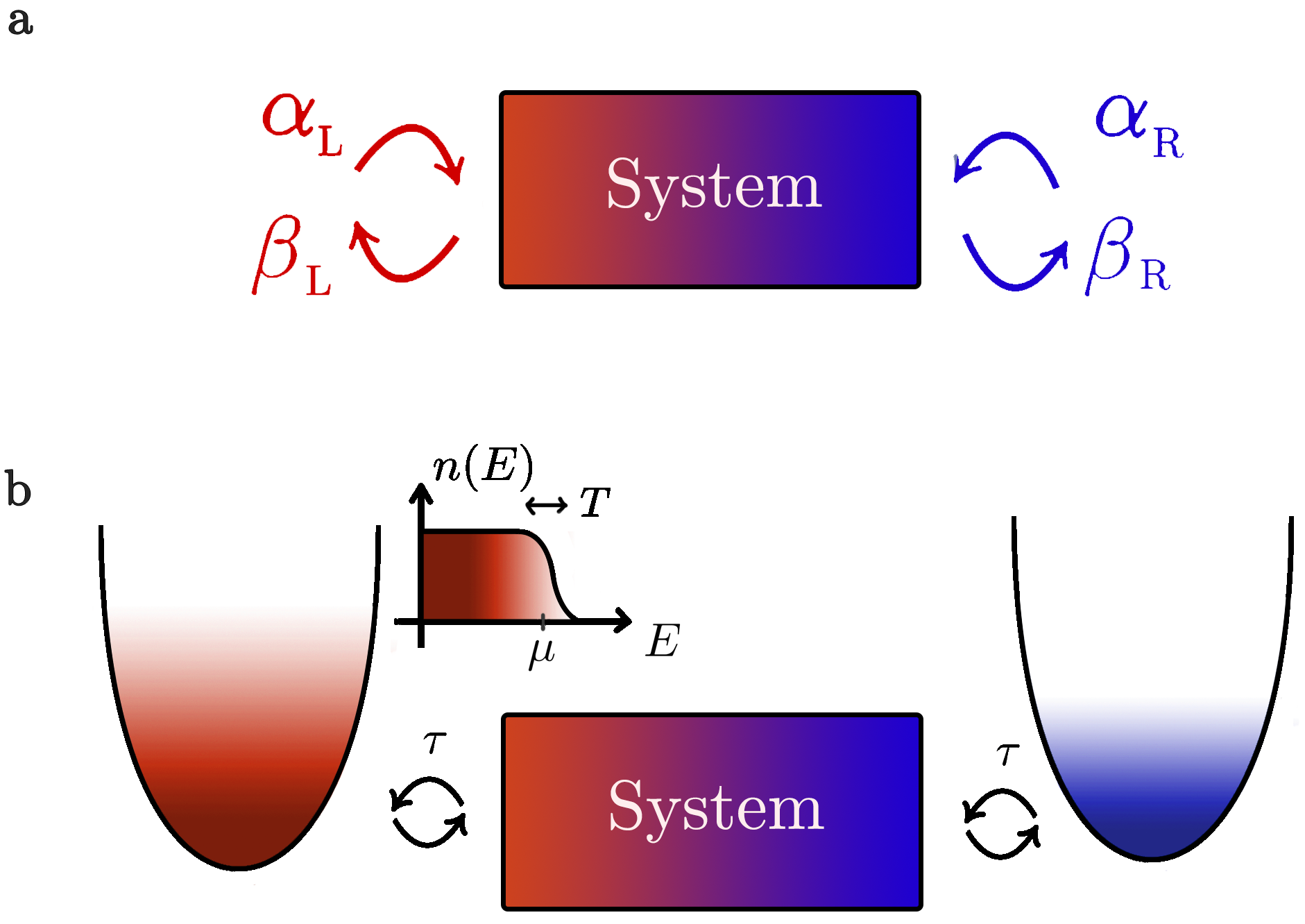
Figure 1: The two type of systems considered in this study. a. System coupled to the exterior via Lindblad-type creation and annihilation operators. There is no knowledge of the structure of the environment. All memory effects are discarded in this setting. b. Explicit coupling to a fermionic bath described at equilibrium by the Fermi-Dirac distribution.

An alternative way to view the coupling of a quantum system to the external world, used in particular routinely in the context of quantum optics (Breuer and Petruccione, 2002; Gardiner and Zoller, 2000), is to describe the evolution of the system by Lindblad-type generators (Lindblad, 1976; Gorini et al., 1976). Such description consists of Markovian processes by which the system has a non-unitary evolution due to some coupling to the external world. The Lindblad description where the operators would either inject or absorb particles could thus replace the coupling to external fermionic reservoirs in order to generate a steady state current through a quantum system, as depicted in Fig. 1. The Lindblad evolution, fully Markovian, is a priori simpler, although of course not equivalent to the fermionic reservoirs, and as such has been widely used coupled with a Liouvillian formalism (Wichterich et al., 2007; Bertini et al., 2020; Žnidarič, 2010a, b; Prosen, 2011a; Medvedyeva and Kehrein, 2013; Karevski et al., 2013; Buča and Prosen, 2014; Guimarães et al., 2016; Guo and Poletti, 2017; Žnidarič, 2019; Bernard and Jin, 2019; Debnath et al., 2017; Frassek et al., 2020; Damanet et al., 2019a, b; Zerah-Harush and Dubi, 2020), to tackle out of equilibrium issues. Beyond experimental interest, for which the Lindblad coupling is the proper microscopic description, on the theory side, this approach has allowed to unveil non-trivial properties of highly excited and correlated systems: integrable structures, traditionally restrained to closed systems in the quantum realm (Prosen, 2008; Medvedyeva et al., 2016; Ziolkowska and Essler, 2020; Bernard and Jin, 2020); the existence of ballistics spin-transport Zotos et al. (1997); Zotos (1999); Prosen (2011b) and anomalous diffusion Gopalakrishnan and Vasseur (2019); Žnidarič (2011); Ljubotina et al. (2017) in the integrable XXZ model, thus allowing for the discovery of Kardar-Parisi-Zhang correlations Kardar et al. (1986); Kriecherbauer and Krug (2010) in the quantum realm Ljubotina et al. (2019); De Nardis et al. (2020); Jin et al. (2020); Bernard and Doussal (2020). Additionally, it has allowed to characterize the anomalous transport properties of disordered  Žnidarič et al. (2016); Mendoza-Arenas et al. (2019a) and quasi-periodic Žnidarič and Ljubotina (2018) interacting systems, the persistence of ballistic transport in the presence of level repulsion induced by single impurities Brenes et al. (2018, 2020a, 2020b) and ballistic-to-diffusive transition induced by integrability-breaking in finite-sized systems Znidaric (2020); Ferreira and Filippone (2020).

However, the study of transport with Lindblad boundary conditions is mostly done on a case by case basis, and it remains unclear which properties of the interacting region determine the current in systems driven by Lindblad reservoirs. In a similar way, although some connection between the fermionic reservoir description and the Lindblad one can be found in the literature Dorda et al. (2017); Arrigoni and Dorda (2018), generic consequences for the transport properties have not been carried out. In particular, an equivalent of the Meir and Wingreen’s formulation Meir and Wingreen (1992) for Lindblad boundary conditions was not worked out yet, and it is yet unclear whether a systematic evaluation of transport properties in arbitrary Markovian settings is possible.

We address this question in the present paper and develop such formalism. We show, by using a Keldysh description Kamenev (2011); Sieberer et al. (2016) of an arbitrary system in presence of Lindblad boundary conditions injecting and extracting particles, that one can derive a generic transport formula in the spirit of the one of Meir-Wingreen. Quite remarkably, this formula relates the transport properties of an arbitrary system uniquely to its Keldysh Green’s function and the injection/extraction rates of the Lindblad boundaries. We also generalize the transport formula to the case when the system itself can have losses and gains of particles by coupling to other Lindblad reservoirs. We then illustrate the usefulness of our generic formula by deriving the current in various settings, summarized in Fig. 2, and in particular a one dimensional tight-binding chain in presence of losses/gains in the bulk.

The paper is structured as follows. In Sec. II, we introduce the general setup and its description in the Hamiltonian and Lindbladian formulation. In Sec. III, we introduce the Keldysh formalism and compute the effective contribution of reservoirs onto the system in both cases. We show how they map onto each other in the limit of high chemical potential and temperature for the fermionic reservoirs. In Sec. IV, we apply our mapping to derive the generic transport formula for Lindblad type boundaries, and a generic system, potentially containing both interactions and dissipation. In Sec. V, we show applications of our formula to three examples. The two first ones, a single level and a one-dimensional chain, were already studied in the literature by other methods and serve to show how or formula allows to recover easily the previous results. The last example, a one-dimensional chain with dissipation, is to the best of our knowledge new and exhibits unusual properties of the current in presence of the dissipative terms. Sec. VI is the conclusion and perspectives. Finally, several technical points have been put in appendices.

II Models

In this section, we detail the two sets of models that we examine in the present paper, as sketched in Fig. 1a. In the fist class of models, generically denoted by a subscript $\mathcal{L}$, Lindblad jump operators inject and extract particles at the left ($L$) and right ($R$) edge of a generic system at different rates. In the second class, generically denoted by a subscript $\mathcal{F}$, the system exchanges particles with two fermionic baths, at the temperature $T$, with different chemical potential $\mu_{L,R}$.

II.1 Lindblad boundary conditions

For the Lindblad boundary condition, the contact with the environment is described by the action of a Lindblad operator ${\cal L}$ (Gorini et al., 1976; Lindblad, 1976; Breuer and Petruccione, 2002). The non-unitary evolution of the density matrix of the system $\rho_{\rm S}$ obeys the Lindblad master equation

$$\frac{d\rho_{\rm S}}{dt}=-i[H_{{\rm S}},\rho_{{\rm S}}]+{\cal L}(\rho_{{\rm S}})\,,$$ (1)

where $H_{{\rm S}}$ is the Hamiltonian of the system. In general, $\mathcal{L}(\rho)=\sum_{n,m}\lambda_{m,n}(\Lambda_{n}\rho\Lambda_{m}^{\dagger}-\frac{1}{2}\{\Lambda_{m}^{\dagger}\Lambda_{n},\rho\})$ where $\{\}$ denotes anticommutation of generic jump operators $\Lambda_{n}$, acting with rates $\lambda_{m,n}$ on the system. We focus here for simplicity on spinless fermions on a lattice. The extension including additional degrees of freedom is straightforward. The experimentally relevant situation, sketched in Fig. 1, involves an external environment which injects particles at site $r=L/R$ at rates $\alpha_{r}$ and extracts them at rates $\beta_{r}$. Injecting and extracting particles at different rates at each end of the system allows to drive currents through it.

This situation is described by the Lindblad operator Prosen (2008); Medvedyeva et al. (2016); Ziolkowska and Essler (2020); Bernard and Jin (2020); Prosen (2011b); Žnidarič (2011); Ljubotina et al. (2017, 2019); De Nardis et al. (2020); Žnidarič et al. (2016); Mendoza-Arenas et al. (2019a); Žnidarič and Ljubotina (2018); Brenes et al. (2018, 2020a, 2020b); Znidaric (2020); Ferreira and Filippone (2020)

$$\begin{split}{\cal L}(\rho_{\rm S})=\sum_{r=L,R}&\Big{\{}\alpha_{r}\Big{[}2c_{r}^{\dagger}\rho_{\rm S}c_{r}-\{c_{r}c_{r}^{\dagger},\rho_{\rm S}\}\Big{]}\\ &\hskip 10.00002pt+\beta_{r}\Big{[}2c_{r}\rho_{\rm S}c_{r}^{\dagger}-\{c_{r}^{\dagger}c_{r},\rho_{\rm S}\}\Big{]}\Big{\}}\,,\end{split}$$ (2)

in which ($c_{r}$,$c_{r}^{\dagger}$) are fermionic annihilation and creation operators acting on the system on site $r$.

The description (2) of the reservoirs relies on the Markovian approximation, which discards all memory effects and correlations between the system and the environment. This is visible in the fact that the action of ${\cal L}$ only depends on the current state $\rho_{\rm S}$ of the system.

II.2 Fermionic reservoirs

The other canonical description, in particular heavily used in solid-state mesoscopic systems Bruus and Flensberg (2004); Nazarov and Blanter (2009); Akkermans and Montambaux (2007); Moskalets (2011), consists of coupling the system to two free fermionic baths, see Fig.1b. These baths mimic large metallic contacts exchanging particles with the edges $r=L/R$ of the system. This setting is described by a Hamiltonian of the form

$$H=H_{{\rm S}}+H_{\rm F}+H_{\tau}\,,$$ (3)

in which $H_{\rm S}$ is the Hamiltonian of the system and $H_{\rm F}$ the Hamiltonian describing the $L$- and $R$-reservoirs:

$$H_{{\rm F}}=\sum_{k,r\in\{L,R\}}\Big{(}\epsilon_{k}-\mu_{r}\Big{)}a_{k,r}^{\dagger}a_{k,r}\,,$$ (4)

where the $a_{k,r}$ denote the usual fermionic annihilation operators. We assume that these fermions have a continuous spectrum $\epsilon_{k}$ and chemical potential $\mu_{r}$. The exchange of fermions between system and reservoirs is described by the tunnelling Hamiltonian

$$H_{\tau}=-\tau\sum_{k,r\in\{L,R\}}\Big{(}a_{k,r}^{\dagger}c_{r}+{\rm h.c.}\Big{)}\,.$$ (5)

The systems described by (1–2) and (3–5) correspond in general to different physical situations. In general they thus lead to different transport properties. For the case of the Lindblad boundaries the current is controlled by the asymmetry of the injection and extraction rates between the $L$ and $R$ sides. For the fermionic case the current is controlled by the chemical potential difference between the two reservoirs. It is thus interesting to connect these two situations, this would allow to gain physical insight by transferring well-established results obtained in each of the two formulations of the problem.

III Keldysh formulation

In this section we give a Keldysh description Keldysh (1965) of the two situations of the previous section. Using the Keldysh formalism allows us to trace out in both cases the reservoirs and boundary conditions and provides a natural path for connecting the two approaches. Given the fact that the reservoirs are coupled locally at each end of the system, it is enough to consider the case where reservoirs are coupled to a single site to see how its action gets modified. In this case, the system is described by the simple Hamiltonian

$$H_{{\rm S}}=\epsilon_{0}c^{\dagger}c\,,$$ (6)

in which $\epsilon_{0}$ describes the local chemical potential for the site occupation.

We operate in the Keldysh path-integral formalism  (Kamenev, 2011; Altland and Simons, 2006), that we summarize here mainly to fix notations. The object of interest is the Keldysh action $\mathcal{S}$, appearing in the partition function $\mathcal{Z}$ of the system:

$$\mathcal{Z}=\int{\cal D}[\psi,\bar{\psi}]e^{i\mathcal{S}[\psi,\bar{\psi}]}\,.$$ (7)

We assume implicitly the standard Keldysh matrix structure in which $\psi=(\psi^{+},\psi^{-})$ are vectors of fermionic Grassmann variables defined on the upper and lower Keldysh branches $\mathcal{C}_{\pm}$. We also follow the Larkin and Ovchinnikov convention (Larkin and Ovchinnikov, 1977) to perform the Keldysh rotation.

In this basis, the Keldysh action is expressed in terms of the retarded, advanced and Keldysh green functions $G^{{\mathcal{R}}}$, $G^{{\mathcal{A}}}$ and $G^{{\mathcal{K}}}$:

$$\mathcal{S}=\int\frac{d\epsilon}{2\pi}(\bar{\psi}^{1},\bar{\psi}^{2})_{(\epsilon)}\begin{pmatrix}[G^{{\mathcal{R}}}]^{-1}&[G^{-1}]^{{\mathcal{K}}}\\ 0&[G^{{\mathcal{A}}}]^{-1}\end{pmatrix}_{(\epsilon)}\begin{pmatrix}\psi^{1}\\ \psi^{2}\end{pmatrix}_{(\epsilon)}\,.$$ (8)

For the single-site Hamiltonian (6), initially at thermodynamic equilibrium of temperature $T_{\rm S}$ and chemical potential $\mu_{\rm S}$, the Green functions read

$$[G_{{\rm S}}^{{\mathcal{R}(\mathcal{A})}}]^{-1} =\epsilon-\epsilon_{0}\pm i\eta\,,$$ (9)

$$G_{{\rm S}}^{{\mathcal{K}}} =-2\pi i\tanh\left(\frac{\epsilon-\mu_{\rm S}}{2T_{{\rm S}}}\right)\delta(\epsilon-\epsilon_{0})\,,$$ (10)

in which $\eta$ is an infinitesimally small quantity. We remind that $[G^{-1}]^{\rm K}=2i\eta\tanh[(\varepsilon-\mu)/2T_{\rm S}]$ is also infinitesimal and formally keeps memory about the initial state of the system Kamenev (2011); Altland and Simons (2006). As we are going to illustrate below, by comparing the effect of adding Lindblad and fermionic reservoirs on the single level, this infinitesimal term can be neglected as soon as the system is coupled to external baths.

III.1 Lindblad reservoirs

In the case of reservoirs described by Lindblad operators as in Eq. (2), the description within the Keldysh formalism is given in Appendix A, following the method outlined in Sieberer et al. (2016). A single reservoir, injecting and extracting particles with rates $\alpha$ and $\beta$, leads to an additional contribution to the action (8), which reads

$$S_{{\cal L}} =i\int\frac{d\epsilon}{2\pi}(\bar{\psi}^{1},\bar{\psi}^{2})_{(\epsilon)}\begin{pmatrix}\alpha+\beta&-2(\alpha-\beta)\\ 0&-(\alpha+\beta)\end{pmatrix}\begin{pmatrix}\psi^{1}\\ \psi^{2}\end{pmatrix}_{(\epsilon)}.$$ (11)

Notice that the upper right element of the action is now finite and the contribution from the initial Keldysh component (10) can be neglected. As an important consequence, the energy of the single level $\epsilon_{0}$ fully disappears from the action, by making the shift $\epsilon\to\epsilon+\epsilon_{0}$ in the integral. This has direct consequences for a certain number of physical properties of the system which will become fully controlled by the bath. For instance, for the case of a single site, the level occupation in the stationary state is given, in terms of Green functions, by

$$\langle n\rangle_{\infty}=\frac{i}{2}\int\frac{d\epsilon}{2\pi}\Big{[}G^{{\mathcal{R}}}(\epsilon)-G^{{\mathcal{A}}}(\epsilon)-G^{{\mathcal{K}}}(\epsilon)\Big{]}\,,$$ (12)

where the Green functions are derived by inverting the full action obtained by adding (8) and (11). One obtains, in the case of Lindblad boundaries Arrigoni and Dorda (2018):

$$\langle n\rangle_{\infty}^{{\cal L}}=\frac{\alpha}{\alpha+\beta},$$ (13)

which exclusively depends on the injection and extraction rates $\alpha$ and $\beta$, irrespective of the local chemical potential $\epsilon_{0}$. The Lindblad case will thus “erase” certain characteristics of the system.

It is also interesting to note that in (11) the retarded and advanced parts of the action depend only on the sum $\alpha+\beta$ and thus are insensitive on whether the boundary condition is injecting or extracting particles. The difference between extraction and injection only appears in the Keldysh component. As we will see below, this has remarkable consequences on some transport properties of systems with losses.

III.2 Fermionic reservoirs

In the case of a fermionic bath, it is useful to obtain simple analytical expressions by making certain approximations on the properties of the reservoirs which correctly describe typical metallic contacts, without loss of generality. In particular, we assume in what follows that the reservoir has a constant density of states. We also make the approximation that the tunnelling takes place on a single site of the system so that the momentum is not conserved during the tunnelling.

These two assumptions allow us to analytically integrate over the reservoirs in (3) and obtain the effective boundary terms for the system. The details of this derivation are given in Appendix B. The single level action thus becomes (we adopt the convention $e=\hbar=k_{B}=1$):

$$S_{\mathcal{F}}=i\int\frac{d\epsilon}{2\pi}(\bar{\psi}^{1},\bar{\psi}^{2})_{(\epsilon)}\Delta\begin{pmatrix}1&2\tanh(\frac{\epsilon-\mu}{2T})\\ 0&-1\end{pmatrix}\begin{pmatrix}\psi^{1}\\ \psi^{2}\end{pmatrix}_{(\epsilon)}\,,$$ (14)

where we introduced the hybridization constant $\Delta=\tau^{2}/v_{F}$, in which $v_{F}$ is the Fermi velocity of the reservoirs and thus a direct measure of the density of states.

III.3 Mapping between the two boundary conditions

The comparison between (11) and (14) shows that the main difference lies in the $\epsilon$–dependence of the Keldysh component of the action for $S_{\mathcal{F}}$. This energy dependence has for consequence that the fermionic boundary term is non-local in time and thus encodes the memory effects of the fermionic bath. Contrarily, the absence of such energy dependence in the action for the Lindblad boundaries $S_{{\mathcal{L}}}$ is directly encoding the Markovian aspect.

It is possible to get rid of the $\epsilon$ dependence of the fermionic reservoirs by taking the limit $\mu\to\infty$, $T\to\infty$, while keeping the ratio $\mu/T$ fixed. One thus obtains the mapping $S_{\mathcal{F}}\to S_{{\cal L}}$ by making the identification

$$\begin{split}\alpha&=\frac{1}{2}\Delta\left[1+\tanh\left(\frac{\mu}{2T}\right)\right]\,,\\ \beta&=\frac{1}{2}\Delta\left[1-\tanh\left(\frac{\mu}{2T}\right)\right]\,.\end{split}$$ (15)

Such limiting mapping between the fermionic reservoirs and the Lindblad boundaries was already noted in general terms in the literature Breuer and Petruccione (2002); Dorda et al. (2017). This precise mapping between the two formalisms allows us to derive the transport properties, as will be done in the next section.

In connection with this limit, it is instructive to consider the single level occupation for the fermionic reservoirs. It is readily derived relying on (12):

$$\langle n\rangle_{\infty}^{{\mathcal{F}}} =\int\frac{d\epsilon}{2\pi}\left[1-\tanh\left(\frac{\epsilon-\mu}{2T}\right)\right]\frac{\Delta}{(\epsilon-\epsilon_{0})^{2}+\Delta^{2}}\,.$$ (16)

First we note that in the limit $\Delta\to 0$ the coupling to the reservoirs becomes extremely small. The density then becomes:

$$\lim_{\Delta\to 0}\langle n\rangle_{\infty}^{{\mathcal{F}}}=\frac{1}{1+e^{\frac{\epsilon_{0}-\mu}{T}}}\,.$$ (17)

In that case we recover the Fermi-Dirac distribution for a single site with energy $\epsilon_{0}$ and at a temperature of the reservoirs, showing that in this limit the only effect of the reservoirs is to thermalize the single site. Note that in our formalism we always implicitly take first the limit of infinitely long time and assume that we have reached a stationary state before taking other limits.

On the other hand, if we take the infinite chemical potential and temperature limit (15), we get back the Lindblad result (13), as can be expected. It is however important to stress that the spectrum of the system has to be bounded to allow to take such limit. In the specific case of the single site case considered in (16), the condition $\mu,T\gg\Delta,\epsilon_{0}$ is sufficient to enforce the correspondence with (13).

IV Generic transport formula for Lindblad boundaries

We are now in a position to tackle the main question of the paper, namely a generic transport formula for Lindblad ($\mathcal{L}$) type boundaries.

IV.1 Generic formula

Let us thus consider a generic quantum system driven out of equilibrium by a a $L$- and $R$- fermionic reservoir (see Fig. 1). Since we want to be able to address the more general case in which the system itself can potentially lose or gain particles, we define two currents

$$\frac{dn_{L}}{dt}=-J_{L},\quad\frac{dn_{R}}{dt}=J_{R}\,,$$ (18)

in which $n_{L/R}$ is the occupation of the sites $L/R$ attached to the reservoirs $L/R$. As a consequence, $J_{L}$ is the current leaving the left reservoir, while $J_{R}$ is the one entering the right reservoir. As a result two generic currents can be defined: $J=(J_{L}+J_{R})/2$ is the current going through the system, while $J_{D}=(J_{L}-J_{R})$ is the current representing the loss (or gain) of particles in the bulk. In the absence of such extraction or injection of charges in the system $J_{D}=0$ and $J$ is the usual conserved current. Let $\boldsymbol{G^{a}}$ with $a\in\{\mathcal{R},\mathcal{A},\mathcal{K}\}$, be the matrices whose elements are the different Green’s function in a given basis. A generic derivation of the current for Lindblad boundary conditions ($\mathcal{L}$) is presented in Appendix C and leads to

$$J_{{\cal L}} =\frac{1}{2}\left\{\big{(}\alpha_{L}-\beta_{L}-\alpha_{R}+\beta_{R}\big{)}+\frac{i}{2}\int\frac{d\epsilon}{2\pi}{\rm Tr}\Big{[}\Big{(}(\alpha_{L}+\beta_{L})\boldsymbol{\gamma_{L}}-(\alpha_{R}+\beta_{R})\boldsymbol{\gamma_{R}}\Big{)}\boldsymbol{G^{{\mathcal{K}}}}\Big{]}\right\}\,,$$ (19)

$$J_{D,{\cal L}} =\frac{i}{2}\int\frac{d\epsilon}{2\pi}{\rm Tr}\Big{[}\Big{(}(\alpha_{L}+\beta_{L})\boldsymbol{\gamma_{L}}+(\alpha_{R}+\beta_{R})\boldsymbol{\gamma_{R}}\Big{)}\boldsymbol{G^{\mathcal{K}}}\Big{]}.$$ (20)

with $\gamma_{r,ij}=2\delta_{i,r}\delta_{i,j}$ in the position basis. This is the main result of the paper.

While Appendix C presents the full derivation of (19–20), we show in the main text how one can also derive (19) by using the mapping (15) and the MW formula for fermionic reservoirs ($\mathcal{F}$). We consider the Hamiltonian of the system in the form $H_{\rm S}=H_{0}+V$, in which $H_{0}=\sum_{i,j}c^{\dagger}_{i}h_{i,j}c_{j}$ is the kinetic part of the Hamiltonian written in position basis and $h_{i,j}$ describes hopping between sites $i$ and $j$. The operator $V$ describes many-body interactions. For such a system the MW formula for the current reads (Meir and Wingreen, 1992)

$$\begin{split}J_{{\mathcal{F}}}&=\frac{i}{2}\int\frac{d\epsilon}{2\pi}{\rm Tr}\left\{\left[\left(f_{L}(\epsilon)-\frac{1}{2}\right)\boldsymbol{\Gamma_{L}}-\left(f_{R}(\epsilon)-\frac{1}{2}\right)\boldsymbol{\Gamma_{R}}\right](\boldsymbol{G^{{\mathcal{R}}}}-\boldsymbol{G}^{\boldsymbol{{\mathcal{A}}}})+\frac{1}{2}(\boldsymbol{\Gamma}_{L}-\boldsymbol{\Gamma}_{R})\boldsymbol{G^{{\mathcal{K}}}}\right\}\end{split}$$ (21)

where the matrices $\Gamma_{r,ij}=\Delta_{r}\gamma_{r,ij}$ in position basis describe the coupling between the system and the baths at the edge site $r$, and $f_{r}(\epsilon)$ is the Fermi-Dirac distribution associated to the $r$-bath.

Using the correspondence (15) in (21) one notices that, after performing the transformation, the term between square brackets becomes constant as a function of energy. This allows to use the additional relation

$$i\int\frac{d\epsilon}{2\pi}(\boldsymbol{G^{{\mathcal{R}}}}-\boldsymbol{G^{{\mathcal{A}}}})=\boldsymbol{\mathbb{I}}\,,$$ (22)

which follows from the fermionic anticommutation relations. Using that $\mbox{Tr}[\mathbf{\Gamma}^{r}]=2\Delta_{r}$, we obtain the formula (19) giving the current for a generic system driven by Lindblad boundary conditions. Note that this result is also valid in presence of dissipation in the system (see Appendix C).

One of the remarkable properties of the Lindblad boundary condition is the fact that the current is fully determined by the Keldysh component of the local Green’s function $\boldsymbol{G^{{\mathcal{K}}}}$. Note that the first term in (19) depends on the difference between injection and extraction rates $\alpha-\beta$ for each of the reservoirs. We could naively expect that this difference plays a similar role to the voltage or chemical potential difference for fermionic reservoirs and thus control the current flow. Nevertheless, this term is not sensitive to the properties of the system, which are encoded in the Keldysh Green’s function appearing in the second term. The second term is also sensitive to the sum of the injection and extraction $\alpha+\beta$ rates of each of the reservoirs. These considerations apply also for the current (20), which quantifies dissipative gains and losses in the system. The Keldysh Green function $\boldsymbol{G^{{\mathcal{K}}}}$ is thus the central object to understand transport in dissipative systems driven by Lindblad boundaries, as we will examine in the examples of the next section.

IV.2 Non-interacting systems

As for the case of fermionic reservoirs, a non-interacting and non-dissipative system allows for further simplifications of the transport formula. In that case, we can rely on two additional relations (Caroli et al., 1971):

$$\begin{split}\frac{1}{2}(&\boldsymbol{G^{{\mathcal{A}}}-G^{{\mathcal{R}}}+G^{{\mathcal{K}}}})=\\ &if_{L}(\epsilon)\boldsymbol{G^{{\mathcal{R}}}}\boldsymbol{\Gamma_{L}}\boldsymbol{G^{{\mathcal{A}}}}+if_{R}(\epsilon)\boldsymbol{G^{{\mathcal{R}}}}\boldsymbol{\Gamma_{R}}\boldsymbol{G^{{\mathcal{A}}}}\,,\end{split}$$ (23)

$$\boldsymbol{G^{{\mathcal{R}}}}- \boldsymbol{G^{{\mathcal{A}}}}=i\boldsymbol{G^{{\mathcal{R}}}}(\boldsymbol{\Gamma_{L}}+\boldsymbol{\Gamma_{R}})\boldsymbol{G^{{\mathcal{A}}}}\,,$$ (24)

leading to the following expression for the current in the fermionic and Lindblad setting

$$J_{{\mathcal{F}}} =\int\frac{d\epsilon}{2\pi}\Big{[}f_{L}(\epsilon)-f_{R}(\epsilon)\Big{]}{\rm Tr}\Big{[}\boldsymbol{\Gamma}_{\boldsymbol{R}}\boldsymbol{G^{{\mathcal{R}}}}\mathbf{\Gamma}_{\boldsymbol{L}}\boldsymbol{G^{{\mathcal{A}}}}\Big{]},$$ (25)

$$J_{{\cal L}} =\int\frac{d\epsilon}{2\pi}\Big{[}\alpha_{L}\beta_{R}-\beta_{L}\alpha_{R}\Big{]}{\rm Tr}\Big{[}\boldsymbol{\gamma_{R}G^{{\mathcal{R}}}\gamma_{L}G^{{\mathcal{A}}}}\Big{]}.$$ (26)

In position basis these expressions become:

$$J_{{\mathcal{F}}} =\int\frac{d\epsilon}{2\pi}\Big{[}f_{L}(\epsilon)-f_{R}(\epsilon)\Big{]}4\Delta_{R}\Delta_{L}|G_{L,R}^{{\mathcal{R}}}|^{2}\,,$$ (27)

$$J_{{\cal L}} =\int\frac{d\epsilon}{2\pi}\Big{[}\alpha_{L}\beta_{R}-\beta_{L}\alpha_{R}\Big{]}4|G_{L,R}^{{\mathcal{R}}}|^{2}\,,$$ (28)

where we used the fact that $\boldsymbol{G^{{\mathcal{R}}*}=G^{{\mathcal{A}}}}$ and $\boldsymbol{G^{{\mathcal{R}}}}$ is symmetric.

For the fermionic reservoirs, Eq. (27) reproduces Landauer-Büttiker formula, where the current is directly related to the probability of transmission through the system at a given energy $\epsilon$. The transmission probability is given by the Green’s function $G^{\mathcal{R}}_{L,R}$ connecting the two reservoirs. The expressions of the currents for the Lindblad and the fermionic bath boundaries both depend on this transmission probability. These probabilities coincide for these two cases, as can be seen from Eqs. (8) and (14), by making the identification $\Delta=\alpha+\beta$. It is thus possible to draw a connection between the two driving protocols in terms of transport coefficients.

Indeed, the corresponding formula for Lindblad boundaries allows further simplifications. For non-interacting and non-dissipative systems, the retarded Green function $\boldsymbol{G^{\mathcal{R}}}$ only depends on the hybridization coefficients $\Delta_{r}=\alpha_{r}+\beta_{r}$. This has the remarkable consequence in (28) that the current $J_{\cal L}$ is always linear in the bias $\alpha_{L}\beta_{R}-\beta_{L}\alpha_{R}$. This allows us to exactly connect the linear response for fermionic systems to the Lindblad driving. For the fermionic case, we consider the linear response limit of (25–27), in which $\delta\mu=\mu_{L}-\mu_{R}\rightarrow 0$ and $T_{R}=T_{L}=T$. In this limit, $f_{L}(\epsilon)-f_{R}(\epsilon)\sim-\partial_{\varepsilon}f(\varepsilon)\delta\mu/T$, which, in the limit of large temperatures, scales as $\delta\mu/4T$. We stress again that such limit makes sense if the transmission amplitude ${\rm Tr}\Big{[}\boldsymbol{\Gamma}_{\boldsymbol{R}}\boldsymbol{G^{{\mathcal{R}}}}\mathbf{\Gamma}_{\boldsymbol{L}}\boldsymbol{G^{{\mathcal{A}}}}\Big{]}$ is non-zero only on a finite energy window. In such a high temperature limit the conductance becomes

$$\begin{split}g(T\rightarrow\infty)&=\lim_{\delta\mu\rightarrow 0}\frac{J_{\mathcal{F}}}{\delta\mu}=\frac{1}{4T}\int\frac{d\epsilon}{2\pi}{\rm Tr}\Big{[}\boldsymbol{\Gamma}_{\boldsymbol{R}}\boldsymbol{G^{{\mathcal{R}}}}\mathbf{\Gamma}_{\boldsymbol{L}}\boldsymbol{G^{{\mathcal{A}}}}\Big{]}\,,\end{split}$$ (29)

which vanishes as the inverse temperature $T$, as expected. Comparing (29) with (26), one gets

$$J_{\cal L}=c\,Tg(T\rightarrow\infty)\,,$$ (30)

where $c=(\alpha_{L}\beta_{R}-\beta_{L}\alpha_{R})/4\Delta_{R}\Delta_{L}$ is a constant which depends on the choice of the Lindblad driving. There is thus a perfect connection between the large temperature conductance of a fermionic system and the transport measured with Lindblad driving. Note that the condition of large chemical potential necessary to derive the mapping (15) is not required here, the limit of large temperature is sufficient. Whether such an exact connection applies in the presence of interactions remains an open question, which is left for further investigations.

V Applications

We provide some applications of the general formula (19) for the systems sketched in Fig. 2. We will compute the current for : i) a single site of energy $\epsilon_{0}$ as described by the Hamiltonian (6); ii) a free fermionic chain of $N$ sites; iii) the same free-fermionic chain but with loss or gain terms modelled by injecting or extracting Lindblad terms acting throughout the chain.

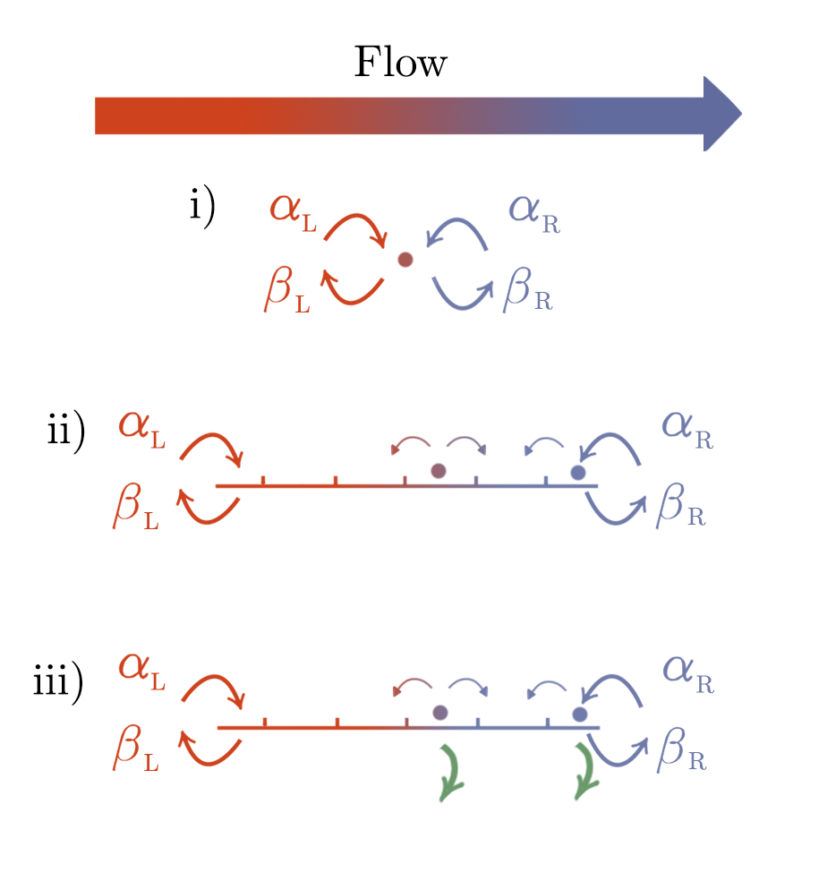
Figure 2: The different situations for which the current is computed with the transport formulae (19–20): i) Single level coupled to reservoirs; ii) Free fermionic chain; iii) Fermionic chain with loss terms along the chain.

i Single site connected to biased reservoirs

A single site connected to biased reservoirs leads to standard Breit-Wigner resonances Breit and Wigner (1936). In this case, $\Gamma_{L/R}=2\Delta_{L/R}$ and the Green function reads, in the case of fermionic bath boundaries, $G^{{\mathcal{R}(\mathcal{A})}}=(\epsilon-\epsilon_{0}\pm i(\Delta_{R}+\Delta_{L}))^{-1}$. Equation (25) leads to the well known result for the current Nazarov and Blanter (2009):

$$J_{{\mathcal{F}}}=\int\frac{d\epsilon}{2\pi}\frac{4\Delta_{R}\Delta_{L}[f_{L}(\epsilon)-f_{R}(\epsilon)]}{(\epsilon-\epsilon_{0})^{2}+(\Delta_{L}+\Delta_{R})^{2}}\,.$$ (31)

For Lindblad type boundaries we have instead

$$G^{{\mathcal{R(A)}}}=(\epsilon-\epsilon_{0}\pm i(\alpha_{R}+\beta_{R}+\alpha_{L}+\beta_{L}))^{-1}\,.$$ (32)

Using the relation 28 for the current leads to

$$J_{{\cal L}}=2e\frac{(\alpha_{L}\beta_{R}-\beta_{L}\alpha_{R})}{\alpha_{L}+\beta_{L}+\alpha_{R}+\beta_{R}}\,.$$ (33)

Comparing (31) and (33) one sees that, as can be expected, all dependence of the current on $\epsilon_{0}$ is lost for the Lindblad case. Thus, the current is fixed entirely by the boundary conditions, in analogy to the occupation (13) of the impurity in the presence of a single Lindblad reservoir. On the other hand, it is clear that for the fermionic baths case, the conductivity depends on the relative values of the chemical potentials of the bath and the Fermi energy of the system.

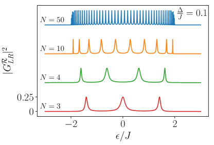
Figure 3: Resonance spectrum (38) of the tight-binding chain as a function of energy and different system sizes $N$. We consider $\Delta/J=0.1$. The plots are shifted vertically for different $N$, for readability.

ii 1D free fermionic chain

The current flowing through a non-interacting fermionic chain attached to Lindblad reservoirs has been recently derived relying on variational (Žnidarič, 2010a) and third-quantization methods Prosen (2008); Guo and Poletti (2017). Our formulation allows to derive the above results in a systematic way relying on standard techniques. Let $N\geq 2$ be the size of the system. The Hamiltonian is $H_{\rm S,chain}=J\sum_{j=1}^{N-1}[c_{j}^{\dagger}c_{j+1}+\mbox{h.c.}]$. According to (31) and (33), we need to compute for fermionic baths boundaries

$${\rm Tr}(\boldsymbol{\Gamma_{R}G^{{\mathcal{R}}}\Gamma_{L}G^{{\mathcal{A}}}})=4\Delta_{R}\Delta_{L}|G_{L,R}^{{\mathcal{R}}}|^{2}$$ (34)

where the indices $L,R$ refer to the sites where the left and right reservoir are connected, i.e $1$ and $N$. For Lindblad boundaries we have similarly

$${\rm Tr}(\boldsymbol{\gamma_{R}G^{{\mathcal{R}}}\gamma_{L}G^{{\mathcal{A}}}})=4|G_{L,R}^{{\mathcal{R}}}|^{2}\,.$$ (35)

In the position basis, for fermionic bath boundaries these functions are given by tridiagonal matrices of the form

$$[\boldsymbol{G}^{\boldsymbol{{\mathcal{R}(\mathcal{A})}}}]^{-1}=\begin{pmatrix}\epsilon+i\Delta_{L}&J&\cdots&0&0\\ J&\epsilon&J&\cdots&0\\ \vdots&J&\ddots&J&\vdots\\ 0&\cdots&J&\epsilon&J\\ 0&0&\cdots&J&\epsilon+i\Delta_{R}\end{pmatrix}\,,$$ (36)

in which the presence of boundaries affects only the first and last diagonal term. The Green functions for Lindblad type boundaries are simply obtained by making the substitution $\Delta_{L}\to\alpha_{L}+\beta_{L}$, $\Delta_{R}\to\alpha_{R}+\beta_{R}$. To simplify notations, we will suppose in what follows that $\Delta_{L}=\Delta_{R}=\Delta$ and $|J|=1$. The inverse of such tridiagonal matrices has been derived in Ref. (Tan, 2019). For the element $(i,j)$ with $i<j$, the Green function reads:

$$G_{i,j}^{{\mathcal{R(A)}}}=(-J)^{i+j}\frac{B_{i-1}^{\mathcal{R(A)}}B_{N-j}^{\mathcal{R(A)}}}{(\epsilon\pm i\Delta)B_{N-1}^{\mathcal{R(A)}}-B_{N-2}^{\mathcal{R(A)}}}\,,$$ (37)

where $B_{i}^{\mathcal{R(A)}}=\frac{(r_{+}\pm i\Delta)r_{+}^{i}-(r_{-}\pm i\Delta)r_{-}^{i}}{(r_{+}\pm i\Delta)-(r_{-}\pm i\Delta)}$ (one has to take the $+$ sign for $\mathcal{R}$ and the $-$ sign for $\mathcal{A}$), and $r^{\pm}_{\epsilon}=(\epsilon\pm\sqrt{\epsilon^{2}-4J^{2}})/2$. Equations (34-37) lead to

$$|G^{\mathcal{R}}_{L,R}(\varepsilon,\Delta)|^{2}=\frac{4|(\epsilon^{2}-4)|}{\bigg{|}(\epsilon-\Delta^{2}\epsilon+4i\Delta)\big{[}(r^{+}_{\epsilon})^{N}-(r^{-}_{\epsilon})^{N}\big{]}+(\Delta^{2}+1)\sqrt{\epsilon^{2}-4}\big{[}(r^{+}_{\epsilon})^{N}+(r^{-}_{\epsilon})^{N}\big{]}\bigg{|}^{2}}\,,$$ (38)

which, inserted in (25-26), gives the current flowing through the system. Equation (38) is plotted in Fig. 3 as a function of energy $\epsilon$. It features $N$ peaks whose width is controlled by the hybridization constant $\Delta$. These peaks correspond to the $N$ single-particle resonances of a chain of $N$ sites, appearing within an energy band of width $4J$.

For the fermionic baths, there is no simple way of carrying the integral in general but, for large values of $N$, there is a simple way of bounding $J_{\mathcal{F}}$ up to corrections of order $e^{-N}$:

$$J_{3}<J_{\mathcal{F}}<J_{1}\,,$$ (39)

with

$$J_{\alpha} =\int_{-\pi/2}^{\pi/2}\frac{d\theta}{\pi}\Big{[}f_{L}(2\sin\theta)-f_{R}(2\sin\theta))\cos^{\alpha}(\theta)\Big{]}$$ (40)

where we took $\Delta=1$ to simplify and made the trigonometric change of variable $\epsilon\to 2\sin\theta$.

For Lindblad boundaries, a numerical evaluation of the expression (28) shows that the current is independent of the system size $N$, namely

$$J_{{\cal L}}=\frac{(\alpha_{L}\beta_{R}-\beta_{L}\alpha_{R})}{\Delta(1+\Delta^{2})}\,,$$ (41)

in agreement with the result of Ref. (Žnidarič, 2010a). As it may be expected for ballistic systems, this result does not depend on the size of the system $N$. Nevertheless, this should be contrasted with the case in which the system is coherently driven by fermionic reservoirs. In this case, the current depends in general on the system size $N$, as it is shown in Fig. 4. This is particularly clear when considering the conductance as defined in Eq. (29), but at zero temperature ($T\to 0$). In this limit, the conductance corresponds to the transmission probability $|G^{\mathcal{R}}_{L,R}(\mu,\Delta)|^{2}$, taken at the chemical potential $\mu$. When plotted as a function of the system size $N$, it displays pronounced even/odd oscillations corresponding to the appearance/disappearance of Fabry-Perot resonances at the energy $\mu=0$ (see also Fig. 3). As expected, and accordingly to the Lindblad limit exemplified by Eq. (30), the size dependence disappears in the $T\rightarrow\infty$ limit, in which the temperature acts as if effectively broadening the single-particle peaks, and making them indistinguishable.

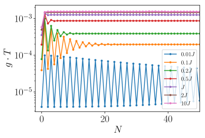
Figure 4: Linear conductance $g$ (29), multiplied by the temperature $T$, as function of the chain size $N$, for $\Delta/J=0.1$ and $\mu=0$ for fermionic baths boundaries. Different colors correspond to different temperatures $T$, listed in the legend.

iii 1D fermionic chain with loss/gain terms

We restrict in this case to Linblad type boundary conditions and add on top of the free fermionic Hamiltonian $H_{S,{\rm chain}}$ the following Lindblad terms in the dynamics $\nu\sum_{j}2c_{j}\rho_{t}c_{j}^{\dagger}-\{c_{j}^{\dagger}c_{j},\rho_{t}\}$, which describes the loss of particles at rate $\nu$ on each site. The gain of particles is instead described by a Lindblad term of the form $\nu\sum_{j}2c^{\dagger}_{j}\rho_{t}c_{j}-\{c_{j}c_{j}^{\dagger},\rho_{t}\}$. Remarkably, the advanced and retarded Green’s functions in the position basis do not discriminate between losses and gains and read, in both cases Dorda et al. (2014):

$$\begin{split}&[\boldsymbol{G}^{\boldsymbol{\mathcal{R}(\mathcal{A})}}]^{-1}=\\ &\begin{pmatrix}\epsilon\pm i\Delta_{L}\pm i\nu&J&\cdots&0&0\\ J&\epsilon\pm i\nu&J&\cdots&0\\ \vdots&J&\ddots&J&\vdots\\ 0&\cdots&J&\epsilon\pm i\nu&J\\ 0&0&\cdots&J&\epsilon\pm i\Delta_{R}\pm i\nu\end{pmatrix}\end{split}$$ (42)

The equivalence of gains and losses for the advanced and retarded Green functions is also apparent in Eq. (11), where the injection/extraction rates $\alpha/\beta$ appears with the same sign on the diagonal.

Importantly, this is not the case for the Keldysh Green function, which, in the case of losses, reads

$$\begin{split}&[\boldsymbol{G}^{\boldsymbol{\mathcal{K}}}]^{-1}=\\ &\begin{pmatrix}-2i((\alpha_{L}-\beta_{L})-\nu)&0&\cdots&0\\ 0&2i\nu&&\vdots\\ \vdots&0&\ddots&0\\ 0&\cdots&0&-2i((\alpha_{R}-\beta_{R})-\nu)\end{pmatrix}\end{split}$$ (43)

while the case with gains is obtained by making the substition $\nu\to-\nu$. Differently from the retarded and advanced components, the Keldysh Green’s function discriminates between losses and gains in the bulk, with important consequences on transport. For instance, the presence of loss/gain terms invalidates the relations (23,24). Thus, standard identities for non-interacting fermion do not apply anymore, but the complexity remains manageable because the loss/gain terms are quadratic in fermionic operators. We thus compute the current from (19). More specifically, we have to compute $G_{1,1}^{\mathcal{K}}$ and $G_{N,N}^{\mathcal{K}}$ (recall that the left site index $L$ is $1$ and the right-site index is $N$ here). As before, we will consider the symmetric case. In addition, to lighten the final formulae we choose $\alpha_{R/L}+\beta_{R/L}=\Delta$ and take $|J|=1$. We also suppose that $\alpha_{L}-\beta_{L}=-(\alpha_{R}-\beta_{R})=\delta\tilde{\mu}$, to be distinguished from the bias in chemical potential $\delta\mu$ in Eq. (29). We also recall the relation $\boldsymbol{G^{\mathcal{K}}}=-\boldsymbol{G^{\mathcal{R}}[G^{\mathcal{K}}]^{-1}G^{\mathcal{A}}}$ (Kamenev, 2011). Since the loss term simply adds a term on the diagonal, we get the inverse of $[\boldsymbol{G}^{\boldsymbol{\mathcal{R}(\mathcal{A})}}]^{-1}$ by making the substitution $\epsilon\to\epsilon\pm i\nu$ in the expression of the inverse for the free case in Section ii.

As it is shown in App. D, it is also in this case possible to reexpress the current as a function of $\boldsymbol{G^{\mathcal{R}}}$, but differently from the Landauer-Büttiker like expressions (27) and (28), namely:

$$J_{{\cal L}}=\delta\tilde{\mu}\left[1+2\Delta\int\frac{d\epsilon}{2\pi}\bigg{(}-|G_{1,1}^{{\rm\mathcal{R}}}|^{2}+|G_{1,N}^{\mathcal{R}}|^{2}\bigg{)}\right]\,.$$ (44)

$G_{i,j}^{\mathcal{R}}$ is given by the expression (37) where one made the substitution $\epsilon\to\epsilon+i\nu$. The behavior of the current with respect to $\nu$ is shown in Fig. 5 for different system sizes. In this case the current does depend on the system size and, for $N>2$, we observe first a decrease of the current and then an increase with respect to the loss of particles $\nu$. For large values of $\nu$ all the curves collapse towards the same value $J_{\mathcal{L}}=\alpha_{R}-\alpha_{L}=\delta\tilde{\mu}$. The reason for this counter-intuitive non-monotonous behavior is due to the fact that, in the large $\nu$ limit, the bulk dynamic doesn’t matter anymore: a particle injected from the left never reaches the right reservoir. As a consequence, the current $J_{L}$ injected from the left is equal to the rate of injection of the left reservoir $2\alpha_{L}$ and, inversely, $J_{R}$ to minus the rate of injection at the right reservoir $2\alpha_{R}$.

Another counterintuitive feature of this model, which is not apparent in Fig. 5, is that the behavior of the current $J_{\mathcal{L}}$ does not discriminate between loss and gain terms. Indeed, $J_{\cal{L}}$ is entirely expressed in terms of elements of $\boldsymbol{G^{\mathcal{R}}}$ (see App. D) which, as previously discussed, has the same expression whether we inject particles at rate $\nu$ along the chain or we extract them. This interesting dependence of the current show that the dissipative model deserves further scrutiny, which will be done in future studies.

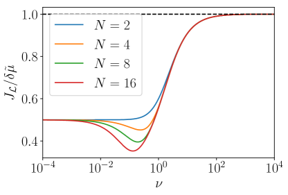
Figure 5: Plot of the behavior of the current as a function of the loss of particles $\nu$ in the system for Lindblad boundary conditions. The different colors correspond to different system sizes $N$. Here $\Delta/J=1$.

Additionally, we can use the formula (20) to compute the current of particles going from the system to the environment. Again, we provide the proof in App. D. It leads to

$$J_{D,{\cal L}}=\pm 4\int\frac{d\epsilon}{2\pi}\sum_{j=1}^{N}\nu\,|G_{1,j}^{\mathcal{R}}|^{2}\,,$$ (45)

where the $+/-$ sign corresponds to the situation in which we consider a loss/gain term weighted by $\nu$ in the Lindbladian. Differently from the direct current $J_{\mathcal{L}}$, the current $J_{D,{\cal L}}$ discriminates between injection or extraction of particles, as expected. For loss terms, we show the behavior of $J_{D,{\cal L}}$ for different system sizes on Fig. 6. For a gain term, we would just have gotten the symmetric of this curve with respect to the horizontal axis. Notice that $J_{D,\mathcal{L}}$ does not depend on the bias $\delta\tilde{\mu}$ and that it tends towards $2$ in the $\nu\rightarrow\infty$ limit.

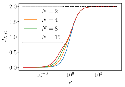
Figure 6: Plot of $J_{D,{\cal L}}$ for Lindblad boundary conditions for different system sizes. We see that as $\nu$ increases, the current leaking from the system to the environment also increases as expected.

VI Conclusion and perspectives

In this work, we derived a generic expression for the stationary current flowing in a general interacting system, potentially with loss or gain of particles, driven by Lindblad jump operators. This expression is the equivalent for Markovian reservoirs of the Meir-Wingreen formula for the fermionic reservoirs. These two situations are related by a limit of high temperature and chemical potential for the fermionic reservoirs. In the non-interacting regime, an additional number of simplifications are possible in this generic transport formula. Using our general transport formula, we showed that, for Lindblad boundaries, the current is always in a linear regime no matter the values of the injecting and extracting rates. We illustrated how our approach can be systematically applied on three different examples concerning non-interacting fermions. For each application, we witnessed drastic differences in the behavior of the current between fermionic bath boundaries and Lindblad ones. Of particular interest is the example of a fermionic tight-binding chain with loss of gain of particles. This system shows a non monotonic dependence of the current in the strength of the dissipation. In addition it has the very counterintuitive feature that the behavior of the current is independent on whether one injects or extracts particles in the bulk.

Our work thus provides a path to tackle transport properties of open systems driven by Lindblad boundaries, with methodology similar to the one used in for mesoscopic systems in contact with fermionic reservoirs and should help bridge the gap between the phenomena in these two situations.

There are of course several directions in which it would be interesting to extend our study.

Concerning the reservoirs, the study of the present paper has been done for Lindbladians that described injection and extraction of particles. It would be interesting to understand whether similar mappings exist for other types of Lindblad action and whether it can be done in a systematic way. For instance, it is possible to generate diffusive behaviors in lattice models of spins or fermions by putting local, independent dephasing noise at each site whose mean actions are described by quartic Lindblad terms Žnidarič and Horvat (2013); Žnidarič (2010c); Bauer et al. (2017); Dolgirev et al. (2020). In this case, the noise is introduced by hand and is supposed to model interaction with an external environment. It would be interesting to make this description more physically grounded by seeing it as emerging from the interaction with an actual environment taken within a certain limit.

Concerning the systems themselves, the models for which we provided explicit evaluations of the transport formulas (19) and (20) here were only non-interacting models. It would be natural to apply our formula to interacting models and give a general interpretation in terms of Keldysh Green functions of the emergence of ballistic and anomalous diffusion in integrable systems Zotos et al. (1997); Zotos (1999); Prosen (2011b); Gopalakrishnan and Vasseur (2019); Žnidarič (2011); Ljubotina et al. (2017). In this spirit, future and interesting research directions could be concerned with single impurity problems Hewson (1993); Bulla et al. (2008); Gull et al. (2011). Given the simplifications that we observed in the studies of this paper for the case of Markovian reservoirs, one can have the hope that tackling such systems will be simpler than for their fermionic counterparts. Finally, extending our approach to describe transport of either matter or energy in interacting systems driven by Lindbladians Mendoza-Arenas et al. (2019b) beyond the strictly one-dimensional case could be tackled by addressing the transport properties in quantum ladder systems.

Appendix A Derivation of the action associated to Lindblad type boundaries

Here, for completeness, we briefly show how to derive (11) from the main text. This derivation was carried out in (Sieberer et al., 2016) and we simply transcribe it here.

Let $\mathfrak{L}$ be the Liouvillian generating the total evolution, i.e $\mathfrak{L}(\rho)=-i[H,\rho]+{\cal L}(\rho)$. where we choose for ${\cal L}$ the injecting and extracting terms introduced in the main text : ${\cal L}(\bullet)=\alpha(2c^{\dagger}\bullet c-\{cc^{\dagger},\bullet\}_{+})+\beta(2c\bullet c^{\dagger}-\{c^{\dagger}c,\bullet\}_{+}$.

By definition

$$\rho_{t}=\lim_{N\to\infty}(\mathbb{I}+\delta t{\cal\mathfrak{L}})^{N}\rho_{0}$$ (46)

with $N\delta t=t$. To get the Keldysh action, we have to insert $2N$ identity resolutions in the above equation, $N$ in the forward direction of time and $N$ in the backward direction of time. The contribution of ${\cal L}$ to the action for an elementary time step is :

$$\left\langle\psi_{n+1}^{+}\right|{\cal L}(\left|\psi_{n}^{+}\right\rangle\left\langle-\psi_{n}^{-}\right|)\left|-\psi_{n+1}^{-}\right\rangle$$ (47)

$$=-\left\langle\psi_{n+1}^{+}|\psi_{n}^{+}\right\rangle\left\langle\psi_{n}^{-}|\psi_{n+1}^{-}\right\rangle$$

$$\hskip 10.00002pt\bigg{(}\alpha(2\bar{\psi}_{n+1}^{+}\psi_{n+1}^{-}+(2-\bar{\psi}_{n+1}^{+}\psi_{n}^{+}-\bar{\psi}_{n}^{-}\psi_{n+1}^{-}))$$

$$\hskip 10.00002pt+\beta(2\psi_{n}^{+}\bar{\psi}_{n}^{-}+(\bar{\psi}_{n+1}^{+}\psi_{n}^{+}+\bar{\psi}_{n}^{-}\psi_{n+1}^{-}))\bigg{)}$$

where $\psi_{n}^{\pm}\bar{\psi}_{n}^{\pm}$ are the usual Grassman fields. Summing over all elementary steps and performing the Keldysh rotation one gets the contribution to the action :

$$S_{{\cal{L}}} =\int\frac{d\epsilon}{2\pi}(\bar{\psi}_{1},\bar{\psi}_{2})_{(\epsilon)}\begin{pmatrix}\alpha+\beta&2(\beta-\alpha)\\ 0&-(\alpha+\beta)\end{pmatrix}\begin{pmatrix}\psi_{1}\\ \psi_{2}\end{pmatrix}_{(\epsilon)}$$ (48)

Appendix B Derivation of the effective action for fermionic bath boundary condition

The starting point is the Hamiltonian (4) from the main text :

$$H =H_{{\rm S}}+H_{{\rm F}}-\mu N_{{\rm F}}+H_{{\rm\tau}},$$

$$H_{{\rm F}} =\sum_{k}\epsilon_{k}\tilde{c}_{{\rm F},k}^{\dagger}\tilde{c}_{{\rm F},k},$$ (49)

$$H_{\tau} =-\tau(c_{{\rm F},0}^{\dagger}c_{\rm F,j}+{\rm h.c}).$$

As explained in the main text, we take the continuous limit in $k$ and the dispersion relation is linearized around the Fermi points

$$\epsilon_{k}=\begin{cases}v_{F}(k-k_{F})&-\Lambda\leq k\leq\Lambda\\ -v_{F}(k+k_{F})&-\Lambda\leq k\leq\Lambda\end{cases}$$ (50)

The total Keldysh action of the full system is composed of three parts,

$$S_{{\rm tot}}=S_{{\rm S}}+S_{{\rm F}}+S_{{\rm\tau}}$$ (51)

The goal is to get an effective action for the system alone by integrating over the degrees of freedom of the bath contained in $S_{{\rm F}}$ and $S_{{\rm\tau}}$.

The Keldysh action for the reservoir is (Kamenev, 2011)

$$S_{\rm F}=$$

$$\int_{-\Lambda}^{\Lambda}\frac{dk}{2\pi}\int\frac{d\epsilon}{2\pi}(\bar{\tilde{\psi}}_{{\rm F}}^{1},\bar{\tilde{\psi}}_{{\rm F}}^{2})_{(\epsilon,k)}\begin{pmatrix}[G_{{\rm F}}^{{\mathcal{R}}}]^{-1}&[G_{{\rm F}}^{-1}]^{{\mathcal{K}}}\\ 0&[G_{{\rm F}}^{{\mathcal{A}}}]^{-1}\end{pmatrix}_{(\epsilon,k)}\begin{pmatrix}\tilde{\psi}_{{\rm F}}^{1}\\ \tilde{\psi}_{{\rm F}}^{2}\end{pmatrix}_{(\epsilon,k)}$$ (52)

with

$$G_{{\rm F}}^{{\mathcal{R(A)}}}(\epsilon,k) =\frac{1}{\epsilon-(\epsilon_{k}-\mu)\pm i\delta},$$ (53)

$$G_{{\rm F}}^{{\mathcal{K}}}(\epsilon,k) =-2\pi i\tanh(\frac{\epsilon-\mu}{2T})\delta(\epsilon-(\epsilon_{k}-\mu)).$$ (54)

where $\delta=0^{+}$.

The Keldysh action associated to $H_{\tau}$ is

$$S_{\tau}=$$

$$\tau\int_{-\Lambda}^{\Lambda}\frac{dk}{2\pi}\int\frac{d\epsilon}{2\pi}\bigg{(}(\bar{\tilde{\psi}}_{{\rm F}}^{1},\bar{\tilde{\psi}}_{{\rm F}}^{2})_{(\epsilon,k)}\begin{pmatrix}\psi_{j}^{1}\\ \psi_{j}^{2}\end{pmatrix}_{(\epsilon)}$$ (55)

$$+(\bar{\psi}_{j}^{1},\bar{\psi}_{j}^{2})_{(\epsilon,k)}\begin{pmatrix}\tilde{\psi}_{{\rm F}}^{1}\\ \tilde{\psi}_{{\rm F}}^{2}\end{pmatrix}_{(\epsilon)}\bigg{)}$$ (56)

Since the theory is quadratic, we can use usual Gaussian integrals formula to integrate over $\tilde{\psi}_{{\rm F}},\bar{\tilde{\psi}}_{{\rm F}}$

$$\int\prod d\bar{\psi}_{j}d\psi_{j}e^{-\sum_{ij}\bar{\psi}_{i}M_{ij}\psi_{j}+\sum_{j}\bar{\psi}_{j}\chi_{j}+\bar{\chi}_{j}\psi_{j}}$$ (57)

$$=\det(M)e^{\sum\bar{\chi}_{i}M_{ij}^{-1}\chi_{j}}$$ (58)

identifying $\psi\to i\begin{pmatrix}\psi^{1}\\ \psi^{2}\end{pmatrix}$, $M\to i\begin{pmatrix}[G_{{\rm F}}^{{\mathcal{R}}}]^{-1}&[G_{{\rm F}}^{-1}]^{{\mathcal{K}}}\\ 0&[G_{{\rm F}}^{{\mathcal{A}}}]^{-1}\end{pmatrix}_{(\epsilon,k)}$, $\chi\to-i\tau\begin{pmatrix}\psi^{1}\\ \psi^{2}\end{pmatrix}_{(\epsilon)}$in the above formula and using $\det(M)=1$ yields the effective action of the bath on the system :

$$S_{\mathcal{F}}=-\int_{-\Lambda}^{\Lambda}\frac{dk}{2\pi}\int\frac{d\epsilon}{2\pi}\tau^{2}(\bar{\psi}_{j}^{1},\bar{\psi}_{j}^{2})_{(\epsilon)}\begin{pmatrix}G_{{\rm F}}^{{\mathcal{R}}}&G_{{\rm F}}^{{\mathcal{K}}}\\ 0&G_{\rm F}^{{\mathcal{A}}}\end{pmatrix}_{(\epsilon,k)}\begin{pmatrix}\psi_{j}^{1}\\ \psi_{j}^{2}\end{pmatrix}_{(\epsilon)}$$ (59)

So we need to compute $\int_{-\Lambda}^{\Lambda}\frac{dk}{2\pi}G_{{\rm F}}^{{\mathcal{R}}({\mathcal{A}})}(\epsilon,k)$ and $\int_{-\Lambda}^{\Lambda}\frac{dk}{2\pi}G_{{\rm F}}^{{\mathcal{K}}}(\epsilon,k)$:

$$\int_{-\Lambda}^{\Lambda}\frac{dk}{2\pi}G_{{\rm F}}^{{\mathcal{R}}({\mathcal{A}})}(\epsilon,k)$$

$$=\int_{-\Lambda}^{\Lambda}\frac{dk}{2\pi}\frac{1}{\epsilon-(\epsilon_{k}-\mu)\pm i\delta}$$

$$=\int_{-\Lambda v_{F}}^{\Lambda v_{F}}\frac{d\epsilon_{k}}{\pi v_{F}}\frac{1}{\epsilon-(\epsilon_{k}-\mu)\pm i\delta}$$

$$=\int_{-\Lambda v_{F}}^{\Lambda v_{F}}\frac{d\epsilon_{k}}{\pi v_{F}}\big{(}{\rm vp}(\frac{1}{\epsilon-(\epsilon_{k}-\mu)})\mp i\pi\delta(\epsilon-(\epsilon_{k}-\mu))\big{)}$$

$$=\frac{1}{\pi v_{F}}(\ln\frac{\epsilon-(-\Lambda v_{F}-\mu)}{\epsilon-(\Lambda v_{F}-\mu)}\mp i\pi)+O(\frac{1}{\Lambda})$$

$$=_{\lim\Lambda\to\infty}\mp\frac{i}{v_{F,L}}.$$ (60)

$$\int_{-\Lambda}^{\Lambda}\frac{dk}{2\pi}G_{{\rm F}}^{{\mathcal{K}}}(\epsilon,k)$$

$$=-\int_{-\Lambda}^{\Lambda}\frac{dk}{2\pi}2\pi i\tanh(\frac{\epsilon-\mu}{2T})\delta(\epsilon-(\epsilon_{k}-\mu))$$

$$=-\int_{-\Lambda v_{F}}^{\Lambda v_{F}}\frac{d\epsilon_{k}}{\pi v_{F}}2\pi i\tanh(\frac{\epsilon-\mu}{2T})\delta(\epsilon-(\epsilon_{k}-\mu))$$

$$=_{\lim\Lambda\to\infty}-\frac{2i}{v_{F}}\tanh(\frac{\epsilon-\mu}{2T}),$$ (61)

which proves (14)

$$S_{{\mathcal{F}}}=i\int\frac{d\epsilon}{2\pi}(\bar{\psi}_{j}^{1},\bar{\psi}_{j}^{2})_{(\epsilon)}\Delta\begin{pmatrix}1&2\tanh(\frac{\epsilon-\mu}{2T})\\ 0&-1\end{pmatrix}\begin{pmatrix}\psi_{j}^{1}\\ \psi_{j}^{2}\end{pmatrix}_{(\epsilon)}$$ (62)

Appendix C Derivation of the transport formula for Lindblad boudaries

In this appendix we give the full derivation of the equation for the current (19) for a generic system, potentially with interactions and loss/gain of particles. The dynamical evolution of the density $n_{L}={\rm tr}(\rho_{t}c_{L}^{\dagger}c_{L})$ of the site connected to the left reservoir is given by

$$\frac{dn_{L}}{dt}=2\alpha_{L}(1-n_{L})-\beta_{L}n_{L}+\mathfrak{L}^{*}(n_{L})$$ (63)

$\mathfrak{L}^{*}$ is the dual of the Liouvillian, generating the time evolution of operators in the Heisenberg picture. The first term corresponds to the current from the reservoir to the site, the second term represents interaction with the rest of the system and/or other external degrees of freedom. In the stationary state, these two are equal. We have a similar equation for the right site:

$$\frac{dn_{R}}{dt}=2\alpha_{R}(1-n_{R})-\beta_{R}n_{R}+\mathfrak{L}^{*}(n_{R})$$ (64)

Hence the stationary current is given by

$$J_{{\cal L}}=\frac{1}{2}(J_{L}+J_{R})$$ (65)

with $J_{L}=2\alpha_{L}(1-n_{L})-\beta_{L}n_{L}$, $J_{R}=-(2\alpha_{R}(1-n_{R})-\beta_{R}n_{R})$.

The expression of the density at site $j$ in terms of Green’s functions is given by $n_{j}=\frac{i}{2}\int\frac{d\epsilon}{2\pi}(G_{j,j}^{{\mathcal{R}}}-G_{j,j}^{{\mathcal{A}}}+G_{j,j}^{{\mathcal{K}}})$. We then have

$$n_{L} =\frac{i}{4}\frac{d\epsilon}{2\pi}{\rm tr}(\boldsymbol{\gamma^{L}}(\boldsymbol{G^{{\mathcal{R}}}}-\boldsymbol{G^{{\mathcal{A}}}}+\boldsymbol{G^{{\mathcal{K}}}}))$$ (66)

$$n_{R} =\frac{i}{4}\frac{d\epsilon}{2\pi}{\rm tr}(\boldsymbol{\gamma^{R}}(\boldsymbol{G^{{\mathcal{R}}}}-\boldsymbol{G^{{\mathcal{A}}}}+\boldsymbol{G^{{\mathcal{K}}}}))$$ (67)

Inserting these two equations in (65) and using that $i\int\frac{d\epsilon}{2\pi}(\boldsymbol{G^{{\mathcal{R}}}}-\boldsymbol{G^{{\mathcal{A}}}})=\boldsymbol{\mathbb{I}}$, we arrive at (19).

Similarly, one can get the current from the chain to the external environment $J_{D,\cal L}=(J_{L}-J_{R})$. When there is no loss in the system, this current is just $0$ by conservation of the number of particle. If $J_{D,\cal L}>0$ it means, that there are loss of particles in the system while if $J_{D,\cal L}<0$, it means that there is a gain of particles in the system. Using again (66,67) and $i\int\frac{d\epsilon}{2\pi}(\boldsymbol{G^{{\mathcal{R}}}}-\boldsymbol{G^{{\mathcal{A}}}})=\boldsymbol{\mathbb{I}}$, we get after some elementary computations that for Lindblad type boundary conditions:

$$J_{D,{\cal L}}=\frac{i}{2}\int\frac{d\epsilon}{2\pi}{\rm tr}(((\alpha_{L}+\beta_{L})\boldsymbol{\gamma_{L}}+(\alpha_{R}+\beta_{R})\boldsymbol{\gamma_{R}})\boldsymbol{G^{\mathcal{K}}}).$$ (68)

which is Eq.(20) of the main text.

Appendix D Transport through dissipative fermionic chains

In this appendix, we provide more details on the calculations presented in Sec. iii.

As explained in the main text, we compute the current from (19). For that, we need to calculate the elements $G_{1,1}^{\mathcal{K}}$ and $G_{N,N}^{\mathcal{K}}$. The starting point is the relation $\boldsymbol{G^{\mathcal{K}}}=-\boldsymbol{G^{{\cal R}}[G^{\mathcal{K}}]^{-1}G^{\mathcal{A}}}$:

$$G_{k,l}^{{\rm\mathcal{K}}}=-\sum_{ij}G_{k,i}^{\mathcal{R}}[G^{\mathcal{K}}]_{i,j}^{-1}G_{j,l}^{\mathcal{A}}$$

$$=\sum_{ij}G_{k,i}^{{\rm\mathcal{R}}}2i\delta_{i,j}\big{(}(\alpha_{L}-\beta_{L})\delta_{i,1}$$ (69)

$$+(\alpha_{R}-\beta_{R})\delta_{i,L}-\nu\big{)}G_{j,l}^{\mathcal{A}}$$

Thus,

$$G_{1,1}^{\mathcal{K}}= 2i\big{(}|G_{1,1}^{\mathcal{R}}|^{2}(\alpha_{L}-\beta_{L})+|G_{1,N}^{\mathcal{R}}|^{2}(\alpha_{R}-\beta_{R})$$ (70)

$$-\sum_{j}\nu|G_{1,j}^{\mathcal{R}}|^{2}\big{)}$$

$$G_{N,N}^{\mathcal{K}}= 2i\big{(}|G_{1,N}^{\mathcal{R}}|^{2}(\alpha_{L}-\beta_{L})+|G_{N,N}^{\mathcal{R}}|^{2}(\alpha_{R}-\beta_{R})$$ (71)

$$-\sum_{j}\nu|G_{j,N}^{\mathcal{R}}|^{2}\big{)}$$

Now let us make the simplifying approximations $\alpha_{L}+\beta_{L}=\alpha_{R}+\beta_{R}=\Delta$, $\alpha_{L}-\beta_{L}=-(\alpha_{R}-\beta_{R})=\delta\tilde{\mu}$. The expression for the current then simplifies into :

$$J_{{\cal L}} =\delta\tilde{\mu}+\frac{i}{2}\Delta\int\frac{d\epsilon}{2\pi}\big{(}G_{1,1}^{\mathcal{K}}-G_{N,N}^{\mathcal{K}}\big{)}\,,$$ (72)

$$J_{D,{\cal L}} =i\Delta\int\frac{d\epsilon}{2\pi}\big{(}G_{1,1}^{\mathcal{K}}+G_{N,N}^{\mathcal{K}}\big{)}$$ (73)

Substituting the found values for $G_{1,1}^{\mathcal{K}}$ and $G_{N,N}^{\mathcal{K}}$ in these last expressions, we arrive at

$$J_{{\cal L}} =\delta\tilde{\mu}-\Delta\int\frac{d\epsilon}{2\pi}\bigg{[}2\delta\tilde{\mu}(|G_{1,1}^{\mathcal{R}}|^{2}-|G_{1,N}^{\mathcal{R}}|^{2})$$ (74)

$$\hskip 10.00002pt-\sum_{j}\nu(|G_{1,j}^{\mathcal{R}}|^{2}-|G_{j,N}^{\mathcal{R}}|^{2})\bigg{]}\,,$$

$$J_{D,{\cal L}} =2\Delta\int\frac{d\epsilon}{2\pi}\sum_{j}\nu\big{(}|G_{1,j}^{\mathcal{R}}|^{2}+|G_{j,N}^{\mathcal{R}}|^{2}\big{)}$$ (75)

Now from (37) one can remark that $G_{1,N-j+1}^{\mathcal{R}}=G_{j,N}^{\mathcal{R}}$. By re indexing the terms in the sum we have that $\sum_{j}|G_{1,j}^{\mathcal{R}}|^{2}=\sum_{j}|G_{j,N}^{\mathcal{R}}|^{2}$ so that :

$$J_{{\cal L}} =\delta\tilde{\mu}\big{(}1-2\Delta\int\frac{d\epsilon}{2\pi}(|G_{1,1}^{\mathcal{R}}|^{2}-|G_{1,N}^{\mathcal{R}}|^{2})\big{)}\,,$$ (76)

$$J_{D,{\cal L}} =4\Delta\int\frac{d\epsilon}{2\pi}\sum_{j}\nu|G_{1,j}^{\mathcal{R}}|^{2}$$ (77)

For gain terms instead of loss terms, the proof follows exactly the same lines. We end up with the same expression for $J_{{\cal L}}$ while

$$J_{D,{\cal L}}=-4\Delta\int\frac{d\epsilon}{2\pi}\sum_{j}\nu|G_{1,j}^{\mathcal{R}}|^{2}$$ (78)

References

- Landauer (1970) R. Landauer, Philosophical magazine 21, 863 (1970).
- Büttiker (1986) M. Büttiker, Physical Review Letters 57, 1761 (1986), publisher: American Physical Society.
- Lesovik and Sadovskyy (2011) G. B. Lesovik and I. A. Sadovskyy, Physics-Uspekhi 54, 1007 (2011).
- Ashcroft (2003) N. W. Ashcroft, Solid State Physics (Thomson Press, New Delhi, 2003).
- Ziman (1960) J. M. Ziman, Electrons and phonons: the theory of transport phenomena in solids (Oxford university press, 1960).
- Coleman (2015) P. Coleman, Introduction to many-body physics (Cambridge University Press, 2015).
- Bruus and Flensberg (2004) H. Bruus and K. Flensberg, Many-Body Quantum Theory in Condensed Matter Physics. An Introduction (Oxford University Press, USA, 2004).
- Nazarov and Blanter (2009) Y. V. Nazarov and Y. M. Blanter, Quantum Transport: Introduction to Nanoscience (Cambridge University Press, Cambridge, 2009).
- Akkermans and Montambaux (2007) E. Akkermans and G. Montambaux, Mesoscopic Physics of Electrons and Photons (Cambridge University Press, 2007).
- Moskalets (2011) M. V. Moskalets, Scattering matrix approach to non-stationary quantum transport (World Scientific, 2011).
- Fitzpatrick et al. (2017) M. Fitzpatrick, N. M. Sundaresan, A. C. Y. Li, J. Koch, and A. A. Houck, Phys. Rev. X 7, 011016 (2017).
- Chiaro et al. (2020) B. Chiaro, C. Neill, A. Bohrdt, M. Filippone, F. Arute, K. Arya, R. Babbush, D. Bacon, J. Bardin, R. Barends, S. Boixo, D. Buell, B. Burkett, Y. Chen, Z. Chen, R. Collins, A. Dunsworth, E. Farhi, A. Fowler, B. Foxen, C. Gidney, M. Giustina, M. Harrigan, T. Huang, S. Isakov, E. Jeffrey, Z. Jiang, D. Kafri, K. Kechedzhi, J. Kelly, P. Klimov, A. Korotkov, F. Kostritsa, D. Landhuis, E. Lucero, J. McClean, X. Mi, A. Megrant, M. Mohseni, J. Mutus, M. McEwen, O. Naaman, M. Neeley, M. Niu, A. Petukhov, C. Quintana, N. Rubin, D. Sank, K. Satzinger, A. Vainsencher, T. White, Z. Yao, P. Yeh, A. Zalcman, V. Smelyanskiy, H. Neven, S. Gopalakrishnan, D. Abanin, M. Knap, J. Martinis, and P. Roushan, arXiv:1910.06024 [cond-mat, physics:quant-ph] (2020), arXiv: 1910.06024.
- Ma et al. (2019) R. Ma, B. Saxberg, C. Owens, N. Leung, Y. Lu, J. Simon, and D. I. Schuster, Nature 566, 51 (2019), number: 7742 Publisher: Nature Publishing Group.
- Dutta and Cooper (2020) S. Dutta and N. R. Cooper, arXiv:2007.08938 [cond-mat] (2020), arXiv: 2007.08938.
- Zajac et al. (2016) D. M. Zajac, T. M. Hazard, X. Mi, E. Nielsen, and J. R. Petta, Physical Review Applied 6, 054013 (2016), publisher: American Physical Society.
- Hensgens et al. (2017) T. Hensgens, T. Fujita, L. Janssen, X. Li, C. J. Van Diepen, C. Reichl, W. Wegscheider, S. Das Sarma, and L. M. K. Vandersypen, Nature 548, 70 (2017), number: 7665 Publisher: Nature Publishing Group.
- Mills et al. (2019) A. R. Mills, D. M. Zajac, M. J. Gullans, F. J. Schupp, T. M. Hazard, and J. R. Petta, Nature Communications 10, 1063 (2019), number: 1 Publisher: Nature Publishing Group.
- Amico et al. (2020) L. Amico, M. Boshier, G. Birkl, A. Minguzzi, C. Miniatura, L.-C. Kwek, D. Aghamalyan, V. Ahufinger, N. Andrei, A. S. Arnold, M. Baker, T. A. Bell, T. Bland, J. P. Brantut, D. Cassettari, F. Chevy, R. Citro, S. De Palo, R. Dumke, M. Edwards, R. Folman, J. Fortagh, S. A. Gardiner, B. M. Garraway, G. Gauthier, A. Günther, T. Haug, C. Hufnagel, M. Keil, W. von Klitzing, P. Ireland, M. Lebrat, W. Li, L. Longchambon, J. Mompart, O. Morsch, P. Naldesi, T. W. Neely, M. Olshanii, E. Orignac, S. Pandey, A. Pérez-Obiol, H. Perrin, L. Piroli, J. Polo, A. L. Pritchard, N. P. Proukakis, C. Rylands, H. Rubinsztein-Dunlop, F. Scazza, S. Stringari, F. Tosto, A. Trombettoni, N. Victorin, K. Xhani, and A. Yakimenko, arXiv:2008.04439 [cond-mat, physics:quant-ph] (2020), arXiv: 2008.04439.
- Amico et al. (2005) L. Amico, A. Osterloh, and F. Cataliotti, Physical Review Letters 95, 063201 (2005), publisher: American Physical Society.
- Seaman et al. (2007) B. T. Seaman, M. Krämer, D. Z. Anderson, and M. J. Holland, Physical Review A 75, 023615 (2007), publisher: American Physical Society.
- Stadler et al. (2012) D. Stadler, S. Krinner, J. Meineke, J.-P. Brantut, and T. Esslinger, Nature 491, 736 (2012).
- Brantut et al. (2012) J.-P. Brantut, J. Meineke, D. Stadler, S. Krinner, and T. Esslinger, Science 337, 1069 (2012).
- Brantut et al. (2013) J.-P. Brantut, C. Grenier, J. Meineke, D. Stadler, S. Krinner, C. Kollath, T. Esslinger, and A. Georges, Science 342, 713 (2013).
- Krinner et al. (2015) S. Krinner, D. Stadler, D. Husmann, J.-P. Brantut, and T. Esslinger, Nature 517, 64 (2015).
- Lebrat et al. (2018) M. Lebrat, P. Grišins, D. Husmann, S. Häusler, L. Corman, T. Giamarchi, J.-P. Brantut, and T. Esslinger, Physical Review X 8, 011053 (2018).
- Jepsen et al. (2020) N. Jepsen, J. Amato-Grill, I. Dimitrova, W. W. Ho, E. Demler, and W. Ketterle, arXiv:2005.09549 [cond-mat, physics:physics, physics:quant-ph] (2020), arXiv: 2005.09549.
- Husmann et al. (2015) D. Husmann, S. Uchino, S. Krinner, M. Lebrat, T. Giamarchi, T. Esslinger, and J.-P. Brantut, Science 350, 1498 (2015).
- Eckel et al. (2014) S. Eckel, F. Jendrzejewski, A. Kumar, C. J. Lobb, and G. K. Campbell, Physical Review X 4, 031052 (2014).
- Eckel et al. (2016) S. Eckel, J. G. Lee, F. Jendrzejewski, C. J. Lobb, G. K. Campbell, and W. T. Hill, Physical Review A 93, 063619 (2016), publisher: American Physical Society.
- Cominotti et al. (2014) M. Cominotti, D. Rossini, M. Rizzi, F. Hekking, and A. Minguzzi, Physical Review Letters 113, 025301 (2014).
- Gutman et al. (2012) D. B. Gutman, Y. Gefen, and A. D. Mirlin, Physical Review B 85, 125102 (2012).
- Filippone et al. (2016) M. Filippone, F. Hekking, and A. Minguzzi, Physical Review A 93, 011602 (2016).
- Papoular et al. (2012) D. J. Papoular, G. Ferrari, L. P. Pitaevskii, and S. Stringari, Physical Review Letters 109, 084501 (2012).
- Simpson et al. (2014) D. P. Simpson, D. M. Gangardt, I. V. Lerner, and P. Krüger, Physical Review Letters 112, 100601 (2014).
- Salerno et al. (2019) G. Salerno, H. M. Price, M. Lebrat, S. Häusler, T. Esslinger, L. Corman, J.-P. Brantut, and N. Goldman, Physical Review X 9, 041001 (2019).
- Filippone et al. (2019) M. Filippone, C.-E. Bardyn, S. Greschner, and T. Giamarchi, Physical Review Letters 123, 086803 (2019).
- Greschner et al. (2019) S. Greschner, M. Filippone, and T. Giamarchi, Physical Review Letters 122, 083402 (2019), arXiv:1809.10927 .
- Nietner et al. (2014) C. Nietner, G. Schaller, and T. Brandes, Physical Review A 89, 013605 (2014).
- Rançon et al. (2014) A. Rançon, C. Chin, and K. Levin, New Journal of Physics 16, 113072 (2014), publisher: IOP Publishing.
- Meir and Wingreen (1992) Y. Meir and N. S. Wingreen, Phys. Rev. Lett. 68, 2512 (1992).
- Breuer and Petruccione (2002) H. P. Breuer and F. Petruccione, The theory of open quantum systems (Oxford University Press, Great Clarendon Street, 2002).
- Gardiner and Zoller (2000) C. Gardiner and P. Zoller, Quantum Noise: A Handbook of Markovian and Non-Markovian Quantum Stochastic Methods with Applications to Quantum Optics, Springer series in synergetics (Springer, 2000).
- Lindblad (1976) G. Lindblad, Communications in Mathematical Physics 48, 119 (1976).
- Gorini et al. (1976) V. Gorini, A. Kossakowski, and E. C. G. Sudarshan, Journal of Mathematical Physics 17, 821 (1976).
- Wichterich et al. (2007) H. Wichterich, M. J. Henrich, H.-P. Breuer, J. Gemmer, and M. Michel, Phys. Rev. E 76, 031115 (2007).
- Bertini et al. (2020) B. Bertini, F. Heidrich-Meisner, C. Karrasch, T. Prosen, R. Steinigeweg, and M. Znidaric, arXiv:2003.03334 [cond-mat, physics:quant-ph] (2020).
- Žnidarič (2010a) M. Žnidarič, Journal of Physics A: Mathematical and Theoretical 43, 415004 (2010a).
- Žnidarič (2010b) M. Žnidarič, Journal of Statistical Mechanics: Theory and Experiment 2010, L05002 (2010b).
- Prosen (2011a) T. Prosen, Phys. Rev. Lett. 106, 217206 (2011a).
- Medvedyeva and Kehrein (2013) M. V. Medvedyeva and S. Kehrein, arXiv e-prints , arXiv:1310.4997 (2013), arXiv:1310.4997 [cond-mat.mes-hall] .
- Karevski et al. (2013) D. Karevski, V. Popkov, and G. M. Schütz, Phys. Rev. Lett. 110, 047201 (2013).
- Buča and Prosen (2014) B. Buča and T. Prosen, Phys. Rev. Lett. 112, 067201 (2014).
- Guimarães et al. (2016) P. H. Guimarães, G. T. Landi, and M. J. de Oliveira, Phys. Rev. E 94, 032139 (2016).
- Guo and Poletti (2017) C. Guo and D. Poletti, Phys. Rev. A 95, 052107 (2017).
- Žnidarič (2019) M. Žnidarič, Physical Review B 99, 035143 (2019), publisher: American Physical Society.
- Bernard and Jin (2019) D. Bernard and T. Jin, Phys. Rev. Lett. 123, 080601 (2019).
- Debnath et al. (2017) K. Debnath, E. Mascarenhas, and V. Savona, New Journal of Physics 19, 115006 (2017), publisher: IOP Publishing.
- Frassek et al. (2020) R. Frassek, C. Giardina, and J. Kurchan, arXiv e-prints , arXiv:2008.03476 (2020), arXiv:2008.03476 [cond-mat.stat-mech] .
- Damanet et al. (2019a) F. Damanet, E. Mascarenhas, D. Pekker, and A. J. Daley, New Journal of Physics 21, 115001 (2019a), publisher: IOP Publishing.
- Damanet et al. (2019b) F. Damanet, E. Mascarenhas, D. Pekker, and A. J. Daley, Physical Review Letters 123, 180402 (2019b), publisher: American Physical Society.
- Zerah-Harush and Dubi (2020) E. Zerah-Harush and Y. Dubi, Phys. Rev. Research 2, 023294 (2020).
- Prosen (2008) T. Prosen, New Journal of Physics 10, 043026 (2008).
- Medvedyeva et al. (2016) M. V. Medvedyeva, F. H. L. Essler, and T. c. v. Prosen, Phys. Rev. Lett. 117, 137202 (2016).
- Ziolkowska and Essler (2020) A. A. Ziolkowska and F. H. Essler, SciPost Phys. 8, 44 (2020).
- Bernard and Jin (2020) D. Bernard and T. Jin, arXiv e-prints , arXiv:2006.12222 (2020), arXiv:2006.12222 [math-ph] .
- Zotos et al. (1997) X. Zotos, F. Naef, and P. Prelovsek, Physical Review B 55, 11029 (1997).
- Zotos (1999) X. Zotos, Physical Review Letters 82, 1764 (1999).
- Prosen (2011b) T. Prosen, Physical Review Letters 106, 2 (2011b), arXiv:1103.1350 .
- Gopalakrishnan and Vasseur (2019) S. Gopalakrishnan and R. Vasseur, Physical Review Letters 122, 127202 (2019).
- Žnidarič (2011) M. Žnidarič, Physical Review Letters 106, 10.1103/PhysRevLett.106.220601 (2011), arXiv:1103.4094 .
- Ljubotina et al. (2017) M. Ljubotina, M. Žnidaric, and T. Prosen, Nature Communications 8, 1 (2017), arXiv:1702.04210 .
- Kardar et al. (1986) M. Kardar, G. Parisi, and Y.-C. Zhang, Physical Review Letters 56, 889 (1986), publisher: American Physical Society.
- Kriecherbauer and Krug (2010) T. Kriecherbauer and J. Krug, Journal of Physics A: Mathematical and Theoretical 43, 403001 (2010), publisher: IOP Publishing.
- Ljubotina et al. (2019) M. Ljubotina, M. Žnidarič, and T. Prosen, Physical Review Letters 122, 210602 (2019), publisher: American Physical Society.
- De Nardis et al. (2020) J. De Nardis, M. Medenjak, C. Karrasch, and E. Ilievski, Physical Review Letters 124, 210605 (2020), publisher: American Physical Society.
- Jin et al. (2020) T. Jin, A. Krajenbrink, and D. Bernard, Phys. Rev. Lett. 125, 040603 (2020).
- Bernard and Doussal (2020) D. Bernard and P. L. Doussal, EPL (Europhysics Letters) 131, 10007 (2020).
- Žnidarič et al. (2016) M. Žnidarič, A. Scardicchio, and V. K. Varma, Physical Review Letters 117, 040601 (2016).
- Mendoza-Arenas et al. (2019a) J. J. Mendoza-Arenas, M. Žnidarič, V. K. Varma, J. Goold, S. R. Clark, and A. Scardicchio, Physical Review B 99, 094435 (2019a), publisher: American Physical Society.
- Žnidarič and Ljubotina (2018) M. Žnidarič and M. Ljubotina, Proceedings of the National Academy of Sciences 115, 4595 (2018).
- Brenes et al. (2018) M. Brenes, E. Mascarenhas, M. Rigol, and J. Goold, Physical Review B 98, 235128 (2018).
- Brenes et al. (2020a) M. Brenes, T. LeBlond, J. Goold, and M. Rigol, (2020a), arXiv:2004.04755 .
- Brenes et al. (2020b) M. Brenes, J. Goold, and M. Rigol, arXiv:2005.12309 [cond-mat] (2020b).
- Znidaric (2020) M. Znidaric, arXiv:2006.09793 [cond-mat, physics:nlin, physics:quant-ph] (2020), arXiv: 2006.09793.
- Ferreira and Filippone (2020) J. S. Ferreira and M. Filippone, arXiv:2006.13891 [cond-mat, physics:quant-ph] (2020), arXiv: 2006.13891.
- Dorda et al. (2017) A. Dorda, M. Sorantin, W. v. d. Linden, and E. Arrigoni, New Journal of Physics 19, 063005 (2017), publisher: IOP Publishing.
- Arrigoni and Dorda (2018) E. Arrigoni and A. Dorda, in Out-of-Equilibrium Physics of Correlated Electron Systems (Springer International Publishing, 2018) pp. 121–188.
- Kamenev (2011) A. Kamenev, Field Theory of Non-Equilibrium Systems (Cambridge University Press, 2011).
- Sieberer et al. (2016) L. M. Sieberer, M. Buchhold, and S. Diehl, Reports on Progress in Physics 79, 096001 (2016).
- Keldysh (1965) L. V. Keldysh, JETP 20, 1018 (1965).
- Altland and Simons (2006) A. Altland and B. Simons, Condensed matter field theory (Cambridge University Press, 2006).
- Larkin and Ovchinnikov (1977) A. Larkin and Y. N. Ovchinnikov, Journal of Experimental and Theoretical Physics 46, 155 (1977).
- Caroli et al. (1971) C. Caroli, R. Combescot, P. Nozieres, and D. Saint-James, Journal of Physics C: Solid State Physics 4, 916 (1971).
- Breit and Wigner (1936) G. Breit and E. Wigner, Physical Review 49, 519 (1936), publisher: American Physical Society.
- Tan (2019) L. S. L. Tan, IMA Journal of Applied Mathematics 84, 679 (2019), https://academic.oup.com/imamat/article-pdf/84/4/679/29027895/hxz010.pdf .
- Dorda et al. (2014) A. Dorda, M. Nuss, W. von der Linden, and E. Arrigoni, Phys. Rev. B 89, 165105 (2014).
- Žnidarič and Horvat (2013) M. Žnidarič and M. Horvat, The European Physical Journal B 86, 67 (2013).
- Žnidarič (2010c) M. Žnidarič, New Journal of Physics 12, 043001 (2010c).
- Bauer et al. (2017) M. Bauer, D. Bernard, and T. Jin, SciPost Phys. 3, 033 (2017).
- Dolgirev et al. (2020) P. E. Dolgirev, J. Marino, D. Sels, and E. Demler, (2020).
- Hewson (1993) A. C. Hewson, The Kondo Problem to Heavy Fermions (Cambridge University Press, Cambridge, 1993).
- Bulla et al. (2008) R. Bulla, T. A. Costi, and T. Pruschke, Reviews of Modern Physics 80, 395 (2008).
- Gull et al. (2011) E. Gull, A. J. Millis, A. I. Lichtenstein, A. N. Rubtsov, M. Troyer, and P. Werner, Rev. Mod. Phys. 83, 349 (2011).
- Mendoza-Arenas et al. (2019b) J. J. Mendoza-Arenas, M. Žnidarič, V. K. Varma, J. Goold, S. R. Clark, and A. Scardicchio, Physical Review B 99, 094435 (2019b), arXiv:1803.11555 .