Abstract

Einstein-Maxwell-scalar models allow for different classes of black hole solutions, depending on the non-minimal coupling function $f(\phi)$ employed, between the scalar field and the Maxwell invariant. Here, we address the linear mode stability of the black hole solutions obtained recently for a quartic coupling function, $f(\phi)=1+\alpha\phi^{4}$ [1]. Besides the bald Reissner-Nordström solutions, this coupling allows for two branches of scalarized black holes, termed cold and hot, respectively. For these three branches of black holes we calculate the spectrum of quasinormal modes. It consists of polar scalar-led modes, polar and axial electromagnetic-led modes, and polar and axial gravitational-led modes. We demonstrate that the only unstable mode present is the radial scalar-led mode of the cold branch. Consequently, the bald Reissner-Nordström branch and the hot scalarized branch are both mode-stable. The non-trivial scalar field in the scalarized background solutions leads to the breaking of the degeneracy between axial and polar modes present for Reissner-Nordström solutions. This isospectrality is only slightly broken on the cold branch, but it is strongly broken on the hot branch.

1 Introduction

The phenomenon of spontaneous scalarization of black holes has received much interest in recent years. In certain scalar-tensor theories, the well-known black holes of General Relativity (GR) remain solutions of the field equations, while in certain regions of the parameter space, additional branches of black hole solutions arise, that are endowed with scalar hair. Spontaneous scalarization can, for instance, be charge-induced, when a scalar field is suitably coupled to the Maxwell invariant $F^{2}$ [2]. Whereas the onset of the instability is universal, the properties of the resulting scalarized black holes and the branch structure of the solutions then depend significantly on the coupling function $f(\phi)$ [1, 2, 3, 4, 5, 6, 7, 8, 9, 10, 11, 12, 13, 14, 15].

Einstein-Maxwell-scalar (EMs) models include two distinctive classes, depending on the choice of $f(\phi)$: models that have black holes with scalar hair only (and do not allow the GR solutions) or models that allow both the GR solutions and new hairy black holes. The latter splits into two further sub-classes: models wherein the GR black holes are unstable, in some region of parameter space, against the tachyonic instability that promotes scalarization and models wherein the GR black holes are never afflicted by this instability. The last two sub-classes have been labelled as classes IIA and IIB, respectively, in [10].

Many previous studies on EMs BHs in the last few years have been motivated by charge-induced spontaneous scalarization, and thus have focused on black holes of class IIA [2, 3, 4, 5, 6, 7, 8, 9, 10, 11, 12, 13, 14, 15]. In the static case, the branch of Reissner-Nordström (RN) black holes then develops a zero mode at a critical charge to mass ratio $q_{\text{cr}}(\alpha)$, that depends on the coupling strength $\alpha$. At this bifurcation point, a new branch of scalarized black holes emerges. The zero mode of the RN black hole branch then turns into an unstable mode, while the new scalarized branch may or may not be stable, depending on the coupling function [3, 5, 9, 14]. Of course, unstable excited scalarized branches exist as well. Let us note at this point that this observed pattern of branches and instabilities is very similar to the one seen in curvature-induced spontaneously scalarized black holes [16, 17, 18, 19, 20, 21, 22, 23, 24, 25, 26, 27, 28, 29, 30, 31, 32, 33].

Recently, we have considered an EMs model employing the quartic coupling function $f(\phi)=1+\alpha\phi^{4}$, which qualifies as class IIB, since the RN branch does not become unstable against scalar perturbations [1]. Instead, we have observed the following interesting pattern: Close to the extremal RN solution, corresponding to the mass to charge ratio $q=1$, a first branch of scalarized black holes emerges. This first branch then exists in the range $q_{\text{min}}(\alpha)\leq q\leq 1$. At $q_{\text{min}}(\alpha)$, it bifurcates with a second branch of scalarized black holes, which extends throughout the interval $q_{\text{min}}(\alpha)\leq q\leq q_{\text{max}}(\alpha)$, and ends in an extremal singular solution at $q_{\text{max}}(\alpha)>1$. Considering the properties of these three branches, we have termed the RN branch as the bald branch, since it does not carry scalar hair, while we have termed the first and the second branches as the cold and the hot branches, respectively, according to the black hole horizon temperatures.

In this first study [1], we have also addressed the radial modes of the black holes for these three branches, since the radial modes signal instabilities with respect to scalar perturbations and thus the onset of scalar hair. While our analysis has shown that there are no unstable radial modes on the RN branch and on the hot scalarized branch, we have found that the cold scalarized branch develops an unstable mode close to the point $q=1$. This instability is present throughout the interval $q_{\text{min}}(\alpha)<q<1$ and ends with a zero mode at the bifurcation point $q_{\text{min}}(\alpha)$ with the hot scalarized branch. Thus, the cold scalarized branch is clearly unstable. However, it remained an open issue whether there are really two stable coexisting branches, the bald RN branch and the hot scalarized branch. This question has motivated our present investigation.

Here, we study linear mode stability of the black holes on all three branches. To that end, we calculate the lowest quasinormal modes for each type of mode. In particular, since the theory has scalar and vector fields coupled to gravity, we have to consider the perturbations of all these fields. In the presence of non-trivial background fields, i.e., when the black hole solutions carry scalar hair and electromagnetic charge, the different types of perturbations generically couple to each other, leading to scalar-led, electromagnetic-led and gravitational-led modes instead of pure scalar, electromagnetic or gravitational modes, which one would find for a Schwarzschild black hole, for instance. Since parity even (polar) and parity odd (axial) perturbations decouple, we arrive at the following set of modes when expanding in spherical harmonics: polar scalar-led $l\geq 0$ modes, axial and polar electromagnetic-led $l\geq 1$ modes, and axial and polar gravitational-led $l\geq 2$ modes.

In Section II, we present the EMs theory studied and the general set of equations. We specify the Ansatz for the spherically symmetric background solutions and give the resulting set of ordinary differential equations (ODEs). We discuss the asymptotic expansions for asymptotically flat black hole solutions with a regular horizon in Section III. Here, we also recall basic properties of the three branches of black hole solutions. In Section IV, we formulate the sets of perturbation equations for spherical, axial and polar perturbations, deferring more details to the Appendix. We present our numerical results for the quasinormal modes in Section V. Here, we show that no further unstable modes arise on any of the three branches. Moreover, we discuss the breaking of isospectrality, i.e., the splitting of the axial and polar electromagnetic-led and gravitational-led modes, caused by the presence of the scalar hair. We conclude in Section V.

2 EMs theory

We consider EMs theory described by the action

$$\mathcal{S}=\int d^{4}x\sqrt{-g}\Big{[}R-2\partial_{\mu}\phi\partial^{\mu}\phi-f(\phi)F_{\mu\nu}F^{\mu\nu}\Big{]}\ ,$$ (1)

where $R$ is the Ricci scalar, $\phi$ is a real scalar field, and $F_{\mu\nu}$ is the Maxwell field strength tensor. The coupling between the scalar and Maxwell fields is determined by the coupling function $f(\phi)$, for which we assume a quartic dependence,

$$f(\phi)=1+\alpha\phi^{4}\ .$$ (2)

For a positive coupling constant $\alpha$, the global minimum of the coupling function is at $\phi=0$.

The set of coupled field equations is obtained via the variational principle and reads

$$R_{\mu\nu}-\frac{1}{2}g_{\mu\nu}R=T_{\mu\nu}^{\phi}+T_{\mu\nu}^{EM}\ ,$$ (3)

$$\nabla_{\mu}(\sqrt{-g}f(\phi)F^{\mu\nu})=0\ ,$$ (4)

$$\frac{1}{\sqrt{-g}}\partial_{\mu}(\sqrt{-g}g^{\mu\nu}\partial_{\nu}\phi)=\dot{f}(\phi)F_{\mu\nu}F^{\mu\nu}\ ,$$ (5)

where $\dot{f}(\phi)=df(\phi)/d\phi$, and $T_{\mu\nu}^{\phi}$ and $T_{\mu\nu}^{EM}$ are the scalar stress-energy tensor and the electromagnetic stress-energy tensor, respectively.

$$T_{\mu\nu}^{\phi}\equiv\frac{1}{2}\partial_{\mu}\phi\partial_{\nu}\phi-\frac{1}{2}g_{\mu\nu}\left(\frac{1}{2}(\partial_{\alpha}\phi)^{2}+V(\phi)\right)\ ,$$ (6)

$$T_{\mu\nu}^{EM}\equiv 2f(\phi)\left(F_{\mu\alpha}F_{\nu}^{\,\,\alpha}-\frac{1}{4}g_{\mu\nu}F^{2}\right)\ .$$ (7)

To construct static spherically symmetric EMs black holes, we employ the line element

$$ds^{2}=-g(r)dt^{2}+\frac{dr^{2}}{1-2m(r)/r}+r^{2}(d\theta^{2}+\sin^{2}\theta d\varphi^{2})\ ,$$ (8)

where the metric functions $g$ and $m$ depend on the radial coordinate $r$. The black holes are supposed to carry electric charge and, in the scalarized case, also scalar charge. We therefore parametrize the gauge potential and the scalar field by

$$A = a_{0}(r)dt\ ,$$

$$\phi = \phi_{0}(r)\ ,$$ (9)

where $a_{0}$ and $\phi_{0}$ are the electric and the scalar field function, respectively, which depend on the radial coordinate $r$. Inserting this Ansatz into the general set of EMs equations (3)-(5), we obtain the following set of ODEs for the functions $g$, $m$, $a_{0}$ and $\phi_{0}$:

$$\partial_{r}\delta = -\frac{r}{4}\,\left(\partial_{r}\phi_{0}\right)^{2}\ ,$$

$$\partial_{r}m = \frac{1}{2}\,f(\phi_{0}){e}^{2\delta}{r}^{2}\left(\partial_{r}a_{0}\right)^{2}+\frac{r}{8}\left(r-2m\right)\left(\partial_{r}\phi_{0}\right)^{2}\ ,$$

$$\partial^{2}_{r}\phi_{0} = \frac{e^{2\delta}r}{r-2m}\left(r(\partial_{r}\phi_{0})f(\phi_{0})-2\dot{f}(\phi_{0})\right)\left(\partial_{r}a_{0}\right)^{2}$$

$$+2\frac{m-r}{\left(r-2m\right)r}(\partial_{r}\phi_{0})\ ,$$

$$\partial^{2}_{r}a_{0} = \left(\frac{1}{4}\,\left(\partial_{r}\phi_{0}\right)^{2}r-\frac{\dot{f}(\phi_{0})}{f(\phi_{0})}(\partial_{r}\phi_{0})-\frac{2}{r}\right)(\partial_{r}a_{0})\ ,$$ (10)

where we have introduced the function $\delta(r)$ via $g=\left(1-\frac{2m}{r}\right)e^{-2\delta}$. Inserting the first equation into the last yields a first integral for the electromagnetic field

$$\partial_{r}a_{0}=\frac{Q}{f(\phi_{0})e^{\delta}r^{2}}\ ,$$ (11)

where $Q$ is the electric charge of the black holes. With this first integral, the above set of equations can be simplified.

3 EMs black holes

We here briefly recall the properties of static spherically symmetric electrically charged EMs black hole solutions with the quartic coupling function (2). First of all, the RN black hole, which is also a solution of the EMs equations, is given by

$$g=1-\frac{2M}{r}+\frac{Q^{2}}{r^{2}}\ ,\ m=M-\frac{Q^{2}}{2r}\ ,\ a_{0}=-\frac{Q}{r}\ ,\ \phi_{0}=0\ .$$ (12)

The scalarized EMs solutions are obtained numerically [1]. Their asymptotic behavior yields their global charges

$$g = 1-\frac{2M}{r}+O(r^{-2})\ ,$$

$$m = M-\left(Q^{2}+Q_{s}^{2}/4\right)\frac{1}{2r}+O(r^{-2})\ ,$$

$$\phi_{0} = \frac{Q_{s}}{r}+\left(MQ_{s}-Q^{2}\frac{\dot{f}(0)}{f(0)}\right)\frac{1}{r^{2}}+O(r^{-3})\ ,$$

$$a_{0} = -\frac{Q}{r}+\frac{QQ_{s}}{2r^{2}}\frac{\dot{f}(0)}{f(0)}+O(r^{-3})\ ,$$ (13)

with black hole mass $M$, electric charge $Q$, and scalar charge $Q_{s}$. Note that there is no conservation law for the scalar field, and that the existence of a horizon imposes a non-trivial relation $Q_{s}=Q_{s}(M,Q)$ [34].

Close to the horizon $r=r_{H}$, the global charges have the expansion

$$g = g_{1}\left(r-r_{H}\right)+O(\left(r-r_{H}\right)^{2})\ ,$$

$$m = \frac{r_{H}}{2}+\frac{Q^{2}}{2r_{H}^{2}f(\phi_{H})}\left(r-r_{H}\right)+O(\left(r-r_{H}\right)^{2})\ ,$$

$$\phi_{0} = \phi_{H}-\frac{2Q^{2}\dot{f}(\phi_{H})}{r_{H}f(\phi_{H})(r_{H}^{2}f(\phi_{H})-Q^{2})}\left(r-r_{H}\right)+O(\left(r-r_{H}\right)^{2})\ ,$$

$$a_{0} = -\Psi_{H}+Q\sqrt{\frac{g_{1}}{r_{H}f(\phi_{H})(r_{H}^{2}f(\phi_{H})-Q^{2})}}\left(r-r_{H}\right)+O(\left(r-r_{H}\right)^{2})\ ,$$ (14)

where $\phi_{0}(r_{H})=\phi_{H}$ and $a_{0}(\infty)-a_{0}(r_{H})=\Psi_{H}$ are the value of the scalar field and the electrostatic potential at the horizon. Further physically relevant horizon properties are, for instance, the temperature $T_{H}$ and the horizon area $A_{H}$, respectively given by

$$T_{H} = \frac{1}{4\pi}\sqrt{\frac{g_{1}}{r_{H}^{3}f(\phi_{H})}(r_{H}^{2}-Q^{2}f(\phi_{H}))}\ ,$$

$$A_{H} = 4\pi r_{H}^{2}\ .$$ (15)

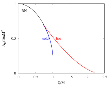
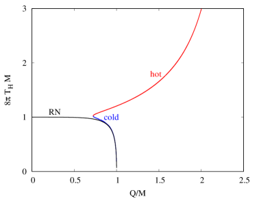
Figure 1: Scalarised black holes (red, blue) for $\alpha=200$ and RN black holes (black): (left) reduced area vs. reduced charge; (right) reduced temperature vs. reduced charge. Scalarised black holes are cold (blue) on the first branch and hot (red) on the second branch.

The EMs black hole solutions can be characterized by three dimensionless quantities: by their charge to mass ratio $q$, their reduced horizon area $a_{H}$ and their reduced horizon temperature $t_{H}$:

$$q\equiv\frac{Q}{M}\ ,\qquad a_{H}\equiv\frac{A_{H}}{16\pi M^{2}}\ ,\qquad t_{H}\equiv 8\pi MT_{H}\ .$$ (16)

In the following we will focus on the case with $\alpha=200$, since for other values of the coupling constant the general properties of the black holes are qualitatively similar. We illustrate the EMs black hole branches in Fig. 1, where we exhibit their reduced area $a_{H}$ (left) and reduced temperature $t_{H}$ (right) versus their charge to mass ratio $q$ [1]. The RN black holes are shown in black. The first scalarized branch emerges close to the extremal RN black hole solution. Along the branch, the mass to charge ratio $q$ decreases, while the reduced area $a_{H}$ and temperature $t_{H}$ increase. At a minimal value of $q$, the first branch bifurcates with the second branch. Along the second branch, $a_{H}$ decreases while $t_{H}$ increases monotonically with increasing $q$. Thus, the first branch represents the cold (blue) branch, and the second branch the hot (red) branch.

4 Linear perturbation theory

Previously, we have addressed the radial stability of these EMs black holes, by looking for radially unstable modes [1]. Our analysis has revealed radial stability for the RN branch and for the hot scalarized branch. In contrast, for the cold scalarized branch, we have found an unstable radial mode. Here, our goal is more ambitious, since we want to fully clarify the linear mode stability of the RN and the hot scalarized branch. As we shall see these are both stable.

To show linear mode stability, we will evaluate the quasinormal mode spectrum of the black holes on these branches. For completeness, we will consider the spectrum on all three branches, including the unstable cold scalarized branch. The symmetry of the background solutions suggests to consider perturbations for the following three cases: purely spherical perturbations ($l=0$), axial or odd-parity ($(-1)^{l+1}$) perturbations, and polar or even-parity ($(-1)^{l}$) perturbations.

4.1 Spherical perturbations

To study the spherical perturbations, we have to perturb all the fields: the scalar field, the electromagnetic field and the metric. For the scalar and the electromagnetic field, we introduce the perturbation functions $\phi_{1}$ and $F_{a_{0}}$, and employ the Ansatz

$$\phi=\phi_{0}(r)+\epsilon e^{-i\omega t}\phi_{1}(r)\ ,$$ (17)

$$A=a_{0}(r)(1+\epsilon e^{-i\omega t}F_{a_{0}}(r))dt\ .$$ (18)

For the metric, we introduce the perturbations functions $F_{t}$ and $F_{r}$ and employ the Ansatz

$$ds^{2}=-g(r)(1+\epsilon e^{-i\omega t}F_{t}(r))dt^{2}+\frac{1+\epsilon e^{-i\omega t}F_{r}(r)}{1-2m(r)/r}dr^{2}+r^{2}(d\theta^{2}+\sin^{2}\theta d\varphi^{2})\ .$$ (19)

We use $\epsilon$ as the control parameter in the linear expansion. The complex quantity $\omega=\omega_{R}+i\omega_{I}$ corresponds to the sought-after eigenvalue of the respective quasinormal mode. Its real part is the oscillation frequency; its imaginary part is the damping rate.

Inserting the Ansatz (17)-(19) into the general set of field equations (3)-(5) and utilizing the set of equations for the background functions (2) leads to the Master equation for the spherical perturbations. This is a single Schrödinger-like ODE for the function $Z=r\phi_{1}$:

$$\frac{d^{2}Z}{d(R^{*})^{2}} = (U_{0}(r)-\omega^{2})Z\ ,$$ (20)

which involves the tortoise coordinate $R^{*}$, where

$$\partial_{r}R^{*} = \frac{1}{\sqrt{g(1-2m/r)}}\ ,$$ (21)

and the potential $U_{0}$, reading

$$U_{0}(r) = \frac{r-2m}{2r^{5}f(\phi_{0})e^{2\delta}}\left[\left(Q^{2}-r^{2}f(\phi_{0})\right)\left(r\partial_{r}\phi_{0}\right)^{2}-4\frac{\dot{f}(\phi_{0})}{f(\phi_{0})}Q^{2}r\partial_{r}\phi_{0}\right.$$ (22)

$$+ \left.2Q^{2}\left(2\left(\frac{\dot{f}(\phi_{0})}{f(\phi_{0})}\right)^{2}-1\right)+4rmf(\phi_{0})\right]\ .$$

To determine the quasinormal modes, we need to impose an adequate set of boundary conditions. As the perturbation propages toward infinity, we have to impose an outgoing wave behavior, i.e.,

$$Z=A_{\phi}^{+}e^{i\omega R^{*}}\left(1+\frac{iM}{2\omega}\frac{1}{r^{2}}+O(r^{-3})\right)\ \,,$$ (23)

for $r\to\infty$. As the perturbation propagates toward the horizon, we have to impose an ingoing wave behavior, i.e.,

$$Z = A_{\phi}^{-}e^{-i\omega R^{*}}$$

$$\left(1+2r_{H}f(\phi_{H})\frac{\left(i\left(\frac{\dot{f}(\phi_{H})}{f(\phi_{H})}\right)^{2}+e^{\delta_{H}}\omega r_{H}\right)Q^{2}-f(\phi_{H})e^{\delta_{H}}\omega r_{H}^{3}}{\left(f(\phi_{H})r_{H}^{2}-Q^{2}\right)\left(-iQ^{2}+f(\phi_{H})r_{H}^{2}(i+2r_{H}e^{\delta_{H}}\omega)\right)}(r-r_{H})+O((r-r_{H})^{2})\right)\,,$$

for $r\to r_{H}$. In these expansions, the quantities $A_{\phi}^{\pm}$ denote arbitrary amplitudes for the perturbation, while all other terms are fixed by the background solution.

4.2 Axial perturbations

When considering axial perturbations, the scalar field does not get affected due to symmetry. Here, only the electromagnetic field and the metric enter. An appropriate Ansatz for the electromagnetic field involves the perturbation function $W_{2}$:

$$A=a_{0}(r)dt-\epsilon W_{2}(r)e^{-i\omega t}\frac{\partial_{\varphi}Y_{lm}(\theta,\varphi)}{\sin{\theta}}d\theta+\epsilon W_{2}(r)e^{-i\omega t}\sin{\theta}{\partial_{\theta}Y_{lm}(\theta,\varphi)}d\varphi\ ,$$ (25)

where $Y_{lm}$ are the standard spherical harmonics. The corresponding Ansatz for the metric

$$ds^{2} = -g(r)dt^{2}+\frac{1}{1-2m(r)/r}dr^{2}+r^{2}(d\theta^{2}+\sin^{2}\theta d\varphi^{2})$$ (26)

$$+2\epsilon h_{0}(r)e^{-i\omega t}\frac{\partial_{\varphi}Y_{lm}(\theta,\varphi)}{\sin{\theta}}dtd\theta+2\epsilon h_{0}(r)e^{-i\omega t}\sin{\theta}\partial_{\theta}Y_{lm}(\theta,\varphi)dtd\varphi$$

$$+2\epsilon h_{1}(r)e^{-i\omega t}\frac{\partial_{\varphi}Y_{lm}(\theta,\varphi)}{\sin{\theta}}drd\theta+2\epsilon h_{1}(r)e^{-i\omega t}\sin{\theta}\partial_{\theta}Y_{lm}(\theta,\varphi)drd\varphi\,,$$

introduces the perturbation functions $h_{0}$ and $h_{1}$.

Inserting this Ansatz into the field equations (3)-(5) leads to a set of coupled differential equations, which is shown in the Appendix. It involves first order equations for the metric perturbation functions $h_{0}$ and $h_{1}$, and a second order equation for the electromagnetic perturbation function $W_{2}$. This system can be put into the form

$$\partial_{r}\Psi_{A}=M_{A}\Psi_{A}\ ,$$ (27)

where $\Psi_{A}$ denotes the perturbation functions in the form

$$\Psi_{A}=\left[\begin{array}[]{c}h_{0}\\ h_{1}\\ W_{2}\\ \partial_{r}W_{2}\end{array}\right]\ ,$$ (32)

and $M_{A}$ denotes a $4\times 4$ matrix which contains the background functions, the angular number $l$, and the eigenvalue $\omega$ of the quasinormal mode. To determine the axial quasinormal modes, as for the radial ones, we have to impose the proper set of boundary conditions at infinity (outgoing) and at the horizon (ingoing). These can be found in the Appendix.

4.3 Polar perturbations

Since the radial perturbations are a set of polar perturbations ($l=0$), it is clear that the general polar perturbations involve again all the fields. For the scalar field, we introduce the perturbation function $\phi_{1}$ and the Ansatz

$$\phi = \phi_{0}(r)+\epsilon e^{-i\omega t}\phi_{1}(r)Y_{lm}(\theta,\varphi)\ .$$ (33)

For the electromagnetic field, we employ the perturbation functions $a_{1}$, $W_{1}$ and $V_{1}$ and the Ansatz

$$A = (a_{0}(r)+\epsilon e^{-i\omega t}a_{1}(r)Y_{lm}(\theta,\varphi))dt+\epsilon W_{1}(r)e^{-i\omega t}Y_{lm}(\theta,\varphi)dr$$ (34)

$$+\epsilon V_{1}(r)e^{-i\omega t}\partial_{\theta}Y_{lm}(\theta,\varphi)d\theta+\epsilon V_{1}(r)e^{-i\omega t}\partial_{\varphi}Y_{lm}(\theta,\varphi)d\varphi\ .$$

Finally, for the metric, we introduce the perturbation functions $N$, $H_{1}$, $L$ and $T$, and employ the Ansatz

$$ds^{2} = -g(r)(1+\epsilon e^{-i\omega t}N(r)Y_{lm}(\theta,\varphi))dt^{2}-2\epsilon e^{-i\omega t}H_{1}(r)Y_{lm}(\theta,\varphi)dtdr+\frac{1-\epsilon e^{-i\omega t}L(r)Y_{lm}(\theta,\varphi)}{1-2m(r)/r}dr^{2}$$ (35)

$$+(r^{2}-2\epsilon e^{-i\omega t}T(r)Y_{lm}(\theta,\varphi))(d\theta^{2}+\sin^{2}\theta d\varphi^{2})\ .$$

Inserting this Ansatz into the field equations (3)-(5) then again results in a set of coupled differential equations, which are shown in the Appendix. In fact, this system of equations can be simplified when one introduces the new functions $F_{0}$, $F_{1}$ and $F_{2}$, that are defined in terms of the perturbation functions $W_{1}$, $V_{1}$ and $a_{1}$ (as discussed in the Appendix). The resulting Master equations can again be put in vectorial form,

$$\partial_{r}\Psi_{P}=M_{P}\Psi_{P}\ .$$ (36)

The vector now contains 6 components:

$$\Psi_{P}=\left[\begin{array}[]{c}H_{1}\\ T\\ F_{0}\\ F_{1}\\ \phi_{1}\\ \partial_{r}\phi_{1}\end{array}\right]\ .$$ (43)

The $6\times 6$ matrix $M_{P}$ depends again on the background functions, the angular number $l$ and the eigenvalue $\omega$ of the quasinormal mode.

We remark that for a RN black hole, the equations for the scalar perturbations are decoupled. However, the equations for the electromagnetic perturbations couple with the equations for the metric perturbations. When the charged black hole also carries scalar hair, all equations are coupled to each other.

Again, we must impose the proper boundary conditions at infinity (outgoing) and at the horizon (ingoing) to determine the quasinormal modes. As in the axial case, these are shown in the Appendix.

5 Quasinormal mode spectrum

In the following, we briefly discuss the method used to extract the quasinormal mode spectrum of the EMs black holes and recall the nomenclature for the modes. Then, we present our numerical results for the $l=0$, $l=1$ and $l=2$ cases and discuss isospectrality breaking.

5.1 Numerics and nomenclature

We calculate the quasinormal modes of the black holes on all three branches, bald, cold and hot, making sure that the respective spectra match, when the background solutions get close. Since the RN quasinormal modes are well-known (see e.g., [35, 36, 37, 38]), this provides an independent check of the numerics used, as well as a first guess for the spectrum of the cold branch, which is typically close to the RN branch for large values of the electric charge. All calculations are performed for a coupling constant $\alpha=200$.

In a first step, we obtain the background solutions with high precision, solving numerically the set of ODEs (2), subject to the boundary conditions following from the expansions at infinity (3) and at the horizon (3). For this purpose, we employ the solver COLSYS [39], which uses a collocation method for boundary-value ODEs together with a damped Newton method of quasi-linearization. The problem is linearized and solved at each iteration step, employing a spline collocation at Gaussian points. The solver features an adaptive mesh selection procedure, refining the grid until the required accuracy is reached.

Once the background solutions are known, we follow the procedure that is analogous to the one we have used before to calculate the quasinormal modes of hairy black holes [32, 33, 40, 41, 42]. We split the space-time into two regions, the inner region $r_{H}+\epsilon_{H}\leq r\leq r_{J}$, and the outer region $r_{J}\leq r\leq r_{\infty}$. In the inner region, we impose the respective ingoing wave behavior; in the outer region, we impose the respective outgoing wave behavior. Then, we calculate sets of linearly independent solutions numerically and match them at the common border $r_{J}$ of the two regions. The eigenvalue $\omega$ of the quasinormal modes is found when the functions and their derivatives are continuous at the matching point $r_{J}$.

We follow a common nomenclature for quasinormal modes, that is used when scalar and electromagnetic fields are coupled in the background solutions. Without such a coupling in the background solutions, one would simply obtain scalar or electromagnetic or gravitational modes by solving the respective scalar, electromagnetic or gravitational perturbation equations, since the different types of perturbations would not be coupled to each other. However, when all fields are already present in the background solutions, the different types of perturbations couple. By taking the respective charges, $Q_{s}$ and $Q$, to zero, the perturbations decouple again. Therefore, we employ a nomenclature that reveals this decoupling limit.

• Modes that are connected with purely scalar perturbations are called scalar-led modes. Typically they have dominant amplitude $A_{\phi}^{\pm}$.

• Modes that are connected with purely electromagnetic perturbations are called EM-led modes. Typically they have dominant amplitude $A_{F}^{\pm}$.

• Modes that are connected with purely gravitational perturbations are called grav-led modes. Typically they have dominant amplitude $A_{g}^{\pm}$.

Scalar-led modes exist for $l\geq 0$, EM-led modes for $l\geq 1$ and grav-led for $l\geq 2$. In the following, we present our results for the quasinormal modes for the cases $l=0$, $1$ and $2$, successively.

5.2 Spectrum of $l=0$ quasinormal modes

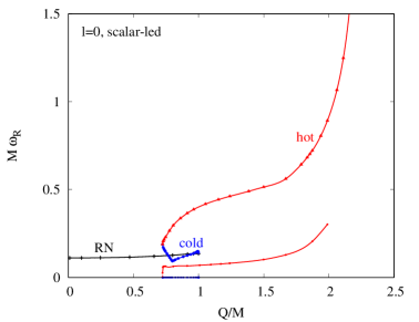
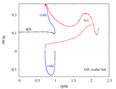
Figure 2: Scalar-led modes for $l=0$ perturbations: scaled real part $\omega_{R}/M$ (a) and scaled imaginary part $-\omega_{I}/M$ (b) vs. reduced charge $q$ for RN (black), and cold (blue) and hot (red) scalarized black holes ($\alpha=200$).

The $l=0$ perturbations are most interesting, since they are the ones that discriminate between stable and unstable EMs black hole solutions. In particular, they feature an unstable mode on the cold black hole branch, whereas the bald and the hot black hole branches possess only stable modes, as our study shows.

We exhibit the lowest scalar-led $l=0$ modes vs. the charge to mass ratio $q$ in Fig. 2, showing the scaled real part of the frequency, $\omega_{R}/M$, in Fig. 2(a) and the scaled imaginary part $-\omega_{I}/M$ in Fig. 2(b). A positive imaginary part signals instability, whereas a negative imaginary part yields the damping time of the mode. Following the color coding of Fig. 1, the bald RN branch is shown in black, the cold EMs branch in blue, and the hot EMs branch in red.

As seen in Fig. 2, the fundamental RN branch has only little dependence on $q$, deviating only slightly from the Schwarzschild mode all the way up to the extremal black hole. The full RN branch is also free of unstable modes.

The cold EMs branch features an unstable scalar-led mode throughout its domain of existence. The mode tend to vanish for the largest charge to mass ratio of the cold branch, $q=1$. The purely imaginary frequency grows as $q$ decreases. At a certain value of $q$ it reaches a maximum, from where it decreases again to the end point of the branch, where it reaches a zero mode. Here the bifurcation with the hot branch is encountered, and thus the minimal charge to mass ratio $q_{\text{min}}$ of both EMs branches is reached. Continuity then requires that at $q_{\text{min}}$, also the hot EMs branch has a zero mode.

Besides the unstable mode, the cold branch features a stable scalar-led mode, which is close to the scalar-led mode of the RN black hole. Along this branch, from $q=1$ to $q_{\text{min}}$ the frequency $\omega_{R}/M$ first decreases slowly and then increases, becoming larger than the frequency of the RN branch, while the damping rate $|\omega_{I}/M|$ increases monotonically.

The corresponding stable scalar-led modes of the hot EMs branch extend from $q_{\text{min}}$ to $q_{\text{max}}$, where an extremal singular EMs solution is reached. The fundamental branch starts at the zero mode at $q_{\text{min}}$, from where both the frequency $\omega_{R}/M$ and the damping rate $|\omega_{I}/M|$ rise at first almost vertically. They continue to rise monotonically, reaching final values above those of the extremal RN branch. The first overtone branch starts at the stable scalar-led mode at the bifurcation point. Its frequency $\omega_{R}/M$ rises also monotonically, but its damping rate $|\omega_{I}/M|$ exhibits an overall but not monotonic decrease.

The reason, we exhibit not only the fundamental stable mode for the hot EMs branch but also the first overtone is to demonstrate continuity of the modes at the bifurcation with the cold EMs branch. The zero mode of the cold EMs branch turns into the fundamental mode of the hot EMs branch, whereas the fundamental mode of the RN branch can be followed via the first stable mode of the cold EMs branch to the first stable overtone of the hot EMs branch.

Of course, all three classical branches feature sequences of (further) overtones, not studied here in detail. In the RN case, they are well known. There, the rapidly damped modes possess several peculiar features. For instance, the higher modes of the non-extremal black holes have been observed to spiral towards the modes of the extremal black hole with increasing $q$ [35, 36].

5.3 Spectrum of $l=1$ quasinormal modes

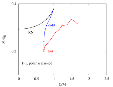
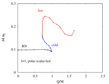
Figure 3: Scalar-led modes for polar $l=1$ perturbations: scaled frequency $\omega_{R}/M$ (a) and scaled damping rate $-\omega_{I}/M$ (b) vs. reduced charge $q$ for RN (black), and cold (blue) and hot (red) scalarized black holes ($\alpha=200$).

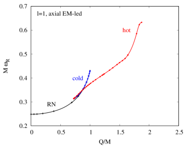
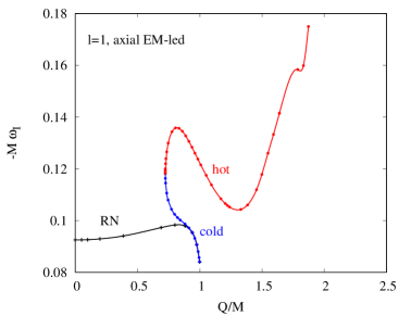
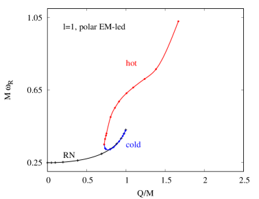
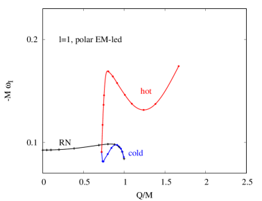
Figure 4: EM-led modes for axial (a)-(b) and polar (c)-(d) $l=1$ perturbations: scaled frequency $\omega_{R}/M$ (a), (c) and scaled damping rate $-\omega_{I}/M$ (b), (d) vs. reduced charge $q$ for RN (black), and cold (blue) and hot (red) scalarized black holes ($\alpha=200$).

The $l=1$ modes consist of polar scalar-led modes and both axial and polar EM-led modes. We start the discussion with the scalar-led modes, shown in Fig. 3. Again, the lowest RN mode changes smoothly with increasing charge to mass ratio $q$. The frequency $\omega_{R}/M$ increases monotonically, while the damping rate $|\omega_{I}/M|$ remains almost constant, showing a slight decrease towards the extremal endpoint $q=1$.

The lowest scalar-led $l=1$ mode of the cold EMs branch changes smoothly from the $q=1$ point to the bifurcation point with the hot EMs branch at $q_{\text{min}}$, exhibiting a monotonic decrease of the frequency $\omega_{R}/M$ and a monotonic increase of damping rate $|\omega_{I}/M|$. Along the hot EMs branch, the change of the eigenvalue with increasing $q$ is no longer monotonic. As compared to the mode of the extremal RN solution, the frequency $\omega_{R}/M$ of the extremal EMs solution is lower and the damping rate $|\omega_{I}/M|$ is higher.

In Fig. 4 we exhibit the axial and polar EM-led $l=1$ modes. The RN black holes are known to exhibit isospectrality, i.e., the axial and polar EM-led modes are degenerate. The EM-led RN modes have an analogous $q$-dependence to the scalar-led RN modes, but their absolute values differ somewhat.

Starting from the $q=1$ bifurcation point, the axial and polar modes of the cold EMs branch follow closely the RN modes at first. The frequencies $\omega_{R}/M$ of both axial and polar modes are slightly higher than the RN frequencies, but do not deviate strongly even at the bifurcation point $q_{\text{min}}$ with the hot EMs branch. The damping rates $|\omega_{I}/M|$ start to deviate from the RN damping rate earlier, showing an opposite behavior for the axial and polar modes. For the axial modes, the damping rates increase monotonically, whereas for the polar modes, a more sinusoidal pattern is seen.

Along the hot EMs branch from $q_{\text{min}}\leq q\leq q_{\text{max}}$, the frequencies $\omega_{R}/M$ of both axial and polar EM-led modes rise monotonically, with the polar frequencies rising almost twice as much compared to the axial ones. The damping rates $|\omega_{I}/M|$ change in a non-monotonic manner again, first rising from the bifurcation point, and then exhibiting some oscillation. At the extremal EMs solution, the damping rates reach similar values, corresponding to about twice the extremal RN value.

5.4 Spectrum of $l=2$ quasinormal modes

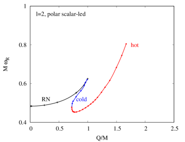
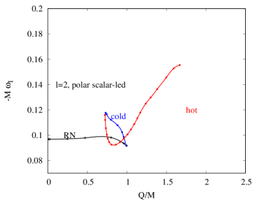
Figure 5: Scalar-led modes for polar $l=2$ perturbations: scaled frequency $\omega_{R}/M$ (a) and scaled damping rate $-\omega_{I}/M$ (b) vs. reduced charge $q$ for RN (black), and cold (blue) and hot (red) scalarized black holes ($\alpha=200$).

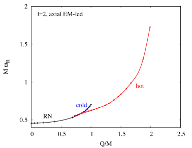
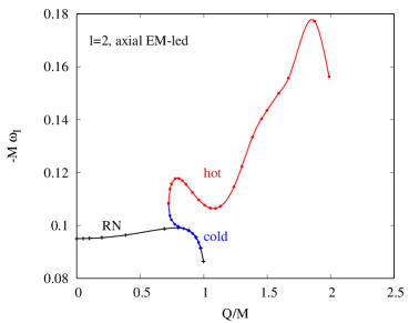
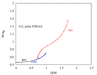
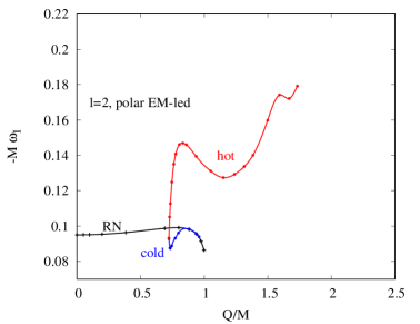
Figure 6: EM-led modes for axial (a)-(b) and polar (c)-(d) $l=2$ perturbations: scaled frequency $\omega_{R}/M$ (a), (c) and scaled damping rate $-\omega_{I}/M$ (b), (d) vs. reduced charge $q$ for RN (black), and cold (blue) and hot (red) scalarized black holes ($\alpha=200$).

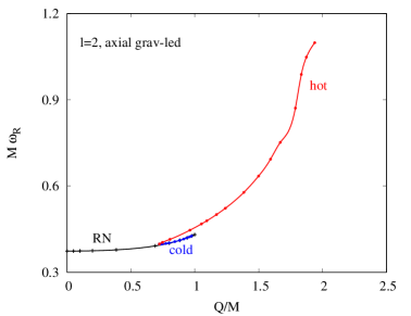
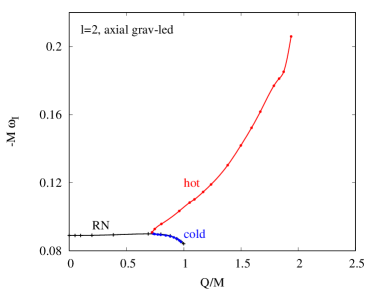
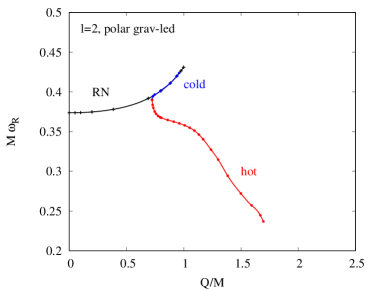
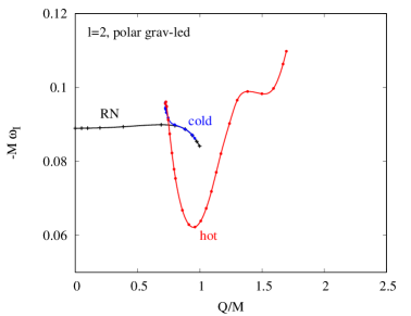
Figure 7: Grav-led modes for axial (a)-(b) and polar (c)-(d) $l=2$ perturbations: scaled frequency $\omega_{R}/M$ (a), (c) and scaled damping rate $-\omega_{I}/M$ (b), (d) vs. reduced charge $q$ for RN (black), and cold (blue) and hot (red) scalarized black holes ($\alpha=200$).

We now turn to the $l=2$ modes, which consist of polar scalar-led modes, axial and polar EM-led modes, and additionally axial and polar grav-led modes. Thus, we now have five types of modes for generic EMs black holes. For the RN case, however, there is again isospectrality of the axial and polar EM-led modes, and there is also isospectrality of the axial and polar grav-led modes. Thus, basically only three types of modes are left, which all show a very similar pattern. It also resembles the pattern seen for $l=0$ and $l=1$. We will therefore now focus the discussion on the more interesting and varied behavior of the modes of the EMs black holes.

As seen in Fig. 5, the scalar-led $l=2$ modes change monotonically on the cold EMs branch. The frequency $\omega_{R}/M$ decreases, and the damping rate $|\omega_{I}/M|$ increases toward the bifurcation point $q_{\text{min}}$. Along the hot EMs branch, the frequency $\omega_{R}/M$ rapidly reaches a minimum and then increases, while the damping rate $|\omega_{I}/M|$ exhibits a sinusoidal behavior. At the extremal EMs solution, both the frequency and the damping rate are higher than that at the extremal RN solution.

The EM-led $l=2$ modes are exhibited in Fig 6. They show a pattern that is very similar to the pattern of the EM-led $l=1$ modes, although the numerical values of the frequencies and damping rates differ, of course. The grav-led $l=2$ modes are exhibited in Fig. 7. The frequencies $\omega_{R}/M$ on the axial and polar cold EMs branches follow very closely the RN branch almost up to the bifurcation point $q_{\text{min}}$. This also holds for the damping rate $|\omega_{I}/M|$ on the axial cold EMs branch. Only the damping rate along the polar EMs branch starts to deviate from the RN one somewhat earlier. Along the hot EMs branch, the frequencies $\omega_{R}/M$ show opposite behavior with the frequency increasing monotonically on the axial branch, while decreasing monotonically along the polar branch. The damping rate $|\omega_{I}/M|$ also increases monotonically along the axial branch, whereas it exhibits a strong sinusoidal behavior along the polar branch.

5.5 Isospectrality

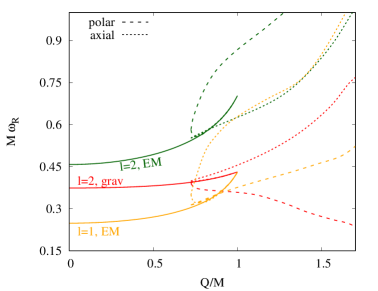
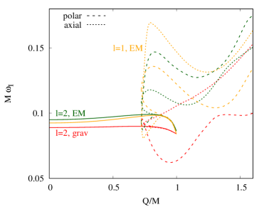
Figure 8: Isospectrality and its breaking for axial (dotted) and polar (dashed) EM-led ($l=1$ yellow, $l=2$ green) and grav-led ($l=2$ red) perturbations: scaled frequency $\omega_{R}/M$ (a) and scaled damping rate $-\omega_{I}/M$ (b) vs. reduced charge $q$ for RN, and cold and hot scalarized black holes ($\alpha=200$).

As addressed in the above discussion, for RN black holes, isospectrality of axial and polar quasinormal modes holds. Here, axial and polar modes coincide for EM-led modes as well as for grav-led modes, for any allowed angular number $l$. Moreover, in the extremal case, the EM-led modes with angular number $l$ agree closely with the grav-led modes with angular number $l+1$ [35, 36]. As seen above and once more highlighted in Fig. 8, this isospectrality survives to a large extent along the cold EMs branch, since the EMs modes follow the RN modes closely over a large range of their existence. In view of Fig. 1, this may, however, not be too surprising, since the cold EMs branch itself follows closely the RN branch almost up to the bifurcation point $q_{\text{min}}$.

In contrast, the hot EMs branch reaches far beyond the RN branch and thus also far beyond the cold EMs branch. Its modes are therefore expected to show a generic behavior on their own. In particular, this branch features a significant background scalar field. The presence of a background scalar field, however, leads to a coupling of all the different perturbations, scalar, vector and gravitational in the polar modes, whereas the axial modes remain free of scalar perturbations. Therefore it should not be surprising that isospectrality gets strongly broken along the hot EMs branch, as illustrated in Fig. 8.

The breaking of isospectrality in the presence of a scalar field has been observed before, of course, notably in Einstein-Maxwell-dilaton black holes [42, 43, 44], and Einstein-scalar-Gauss-Bonnet black holes [32, 33, 40, 41].

6 Conclusion

EMs theories represent an interesting simple setting to study generic properties of spontaneous scalarization of black holes and, more generically, the interplay between bald and hairy black holes. Although the presence of scalar hair is charge-induced, many similarities with the more realistic curvature-induced spontaneous scalarization and scalar hairy black holes have been observed, lending weight to EMs studies beyond an intrinsic theoretical interest.

Here, we have investigated the linear mode stability of EMs black hole solutions with a quadratic coupling function, representing type IIB characteristics: the presence of scalarized black black holes, while the RN branch remains stable throughout. In particular, the system features besides the bald RN branch a cold EMs branch and a hot EMs branch. The cold EMs branch exists in the interval $q_{\text{min}}(\alpha)\leq q\leq 1$, and the hot EMs branch in $q_{\text{min}}(\alpha)\leq q\leq q_{\text{max}}(\alpha)$.

The EMs black holes on the cold branch has an unstable scalar-led mode, present for all $q_{\text{min}}(\alpha)\leq q\leq 1$. At $q_{\text{min}}(\alpha)$, this instability becomes a zero mode that is shared with the hot branch. By continuity, the hot branch then exhibits a stable scalar-led mode, starting at $q_{\text{min}}(\alpha)$.

In our mode analysis, we have calculated the lowest quasinormal modes of all types of perturbations, scalar-led modes, axial and polar EM-led modes, and axial and polar grav-led modes for all three (bald, cold, hot) branches. For the stable modes on the cold EMs branch, we have found close similarity with the respective RN modes, almost up to the bifurcation point with the hot EMs branch $q_{\text{min}}(\alpha)$. Since the cold EMs branch itself follows closely the RN branch, this behavior could have been anticipated. In contrast, the modes of the hot EMs branch show a wide variation and large deviations from the modes of RN branch. But again, the hot EMs branch reaches far beyond the RN branch (for sufficiently large $\alpha$).

RN black holes possess degenerate axial and polar modes in the EM-led and grav-led sectors. As expected, this isospectrality gets broken in the presence of a non-trivial background scalar field, since scalar perturbations contribute in the polar case but not in the axial case. Not surprisingly, the breaking of isospectrality is very limited on the cold EMs branch, but becomes very strong on the hot EMs branch, away from the bifurcation point.

The analysis here has focused on an illustrative value of the coupling $\alpha=200$ and for $\ell=0,1,2$, but the results concerning instability are generic for all values of $\alpha$; moreover, it is not to be expected that higher $l$ modes introduce more instabilities. Thus our analysis has shown that there are no further unstable modes apart from the unstable scalar-led $l=0$ mode of the cold EMs branch. This implies that there are two linearly mode-stable branches in the system, the bald RN branch and the hot EMs branch. While both branches have large regions in parameter space, where their black holes are the only existing black holes, there is also an overlap region $q_{\text{min}}(\alpha)\leq q\leq 1$. Here, both branches coexist and both are mode-stable.

However, when these branches are considered from a thermodynamical point of view, their reduced horizon areas differ except at one critical point $q_{\text{th}}(\alpha)$, where the two curves cross, as seen in Fig. 1. This might suggest that the RN black holes represent the physically preferred state for $0<q<q_{\text{th}}(\alpha)$, whereas the hot EMs black holes represent the physically preferred state for $q_{\text{th}}(\alpha)<q\leq q_{\text{max}}(\alpha)$. Here, dynamical calculations of the EMs evolution equations might give further insight into the interesting question of which type of black hole will represent the end state of collapse in the overlap region.

Acknowledgments

JLBS, SK and JK gratefully acknowledge support by the DFG Research Training Group 1620 Models of Gravity and the COST Action CA16104 GWverse. JLBS would like to acknowledge support from the DFG Project No. BL 1553. AMP is supported by the FCT grant PD/BD/142842/2018. This work was supported by the Center for Research and Development in Mathematics and Applications (CIDMA) through the Portuguese Foundation for Science and Technology (FCT - Fundação para a Ciência e a Tecnologia), references UIDB/04106/2020 and UIDP/04106/2020, by national funds (OE), through FCT, I.P., in the scope of the framework contract foreseen in the numbers 4, 5 and 6 of the article 23, of the Decree-Law 57/2016, of August 29, changed by Law 57/2017, of July 19 and by the projects PTDC/FIS-OUT/28407/2017 and CERN/FIS-PAR/0027/2019. This work has further been supported by the European Union’s Horizon 2020 research and innovation (RISE) programme H2020-MSCA-RISE-2017 Grant No. FunFiCO-777740. We would like to acknowledge networking support by the COST Action GWverse CA16104.

Appendix A Perturbation equations

In this appendix we present the explicit form of the perturbation equations for the axial and polar case, and also the first terms in the asymptotic expansion of the perturbation functions.

A.1 Axial perturbations

By substituting the Ansatz (26) and (25) into the field equations (3)-(5), we obtain a set of differential equations for the axial perturbations:

$$\partial_{r}h_{0}=-i\omega h_{1}-4f(\phi_{0})(\partial_{r}{a_{0}})W_{2}+\frac{2}{r}h_{0}-{\frac{{i}}{2\omega\,{r}^{3}g}h_{1}}\Big{[}-\left(\partial_{r}\phi_{0}\right)^{2}g^{2}{r}^{2}(r-2m)$$

$$-2rg^{2}l(l+1)+2rg\left(\partial_{r}g\right)\left(r\partial_{r}m+m-r\right)-2{r}^{2}g\left(\partial_{r}^{2}g\right)(r-2m)+4{r}^{2}{f(\phi_{0})}g\left(\partial_{r}{a_{0}}\right)^{2}(r-2m)$$

$$+\left(\partial_{r}g\right)^{2}{r}^{2}(r-2m)+4\,\left(\partial_{r}m\right)rg^{2}+4g^{2}(r-m)\Big{]}\ ,$$

$$\partial_{r}h_{1}={\frac{-i\omega rh_{0}}{g\left(r-2m\right)}}+h_{1}\frac{2g\left(\partial_{r}m\right)r-r\left(\partial_{r}g\right)\left(r-2m\right)-2gm}{2rg\left(r-2m\right)}\ ,$$

$$\partial_{r}^{2}{W_{2}}={\left(\frac{4}{g}{f(\phi_{0})}\left(\partial_{r}a_{0}\right)^{2}-\frac{{\omega}^{2}{r}}{g(r-2m)}+\frac{l(l+1)}{r(r-2m)}\right){W_{2}}}-\left[\frac{\partial_{r}g}{2g}-\frac{\partial_{r}m}{r-2m}+\frac{\dot{f}(\phi_{0})}{f(\phi_{0})}\partial_{r}\phi_{0}+\frac{m}{r(r-2m)}\right]{\partial_{r}{W_{2}}}$$

$$+\frac{i(\partial_{r}a_{0})h_{1}}{2\omega r^{3}g^{2}}\Big{[}4g^{2}(r-m)+4rg^{2}\partial_{r}m-r^{2}g^{2}(r-2m)(\partial_{r}\phi_{0})^{2}-2rg^{2}l(l+1)$$

$$+4gr^{2}f(\phi_{0})(r-2m)(\partial_{r}a_{0})^{2}-2gr^{2}(r-2m)(\partial_{r}^{2}g)+r^{2}(r-2m)(\partial_{r}g)^{2}+(2r^{2}g\partial_{r}m+2rg(m-r))\partial_{r}g\Big{]}$$

$$+h_{0}\left[\left(\frac{\partial_{r}g}{2g^{2}}+\frac{\partial_{r}m}{m(r-2m)}-\frac{\dot{f}(\phi_{0})}{f(\phi_{0})}\frac{\partial_{r}\phi_{0}}{g}+\frac{3m-2r}{gr(r-2m)}\right)\partial_{r}a_{0}-\frac{\partial_{r}^{2}a_{0}}{g}\right]\ .$$ (44)

This system of coupled differential equations consists of two first order differential equations for $h_{0}$ and $h_{1}$, plus a second order differential equation for $W_{2}$.

A perturbation with an outgoing wave behavior satisfying this system of equations has to behave like

$$h_{0}=re^{i\omega R}\left[A_{g}^{+}\left(-\omega+O(r^{-1})\right)+A_{F}^{+}\left(\frac{Q}{r^{2}}+O(r^{-3})\right)\right]\ ,$$

$$h_{1}=r\omega e^{i\omega R}\left[A_{g}^{+}\left(1+O(r^{-1})\right)+A_{F}^{+}\left(\frac{-Q}{\omega r^{2}}+O(r^{-3})\right)\right]\ ,$$

$$W_{2}=e^{i\omega R}\left[A_{g}^{+}\left(\frac{Q(l-1)(l+2)}{4\omega r^{2}}+O(r^{-3})\right)+A_{F}^{+}\left(1+O(r^{-1})\right)\right]\ .$$ (45)

In addition, close to the horizon, a perturbation with an ingoing wave behavior has to satisfy

$$h_{0} = e^{-i\omega R}\left[A_{g}^{-}\left(1+O(r-r_{H})\right)+A_{F}^{-}\left(O(r-r_{H})\right)\right]\ ,$$

$$h_{1} = \frac{\omega}{r-r_{H}}e^{-i\omega R}\left[A_{g}^{-}\left(\frac{r_{H}^{3/2}\sqrt{f(\phi_{H})}}{\omega\sqrt{g_{1}\left(r_{H}^{2}f(\phi_{H})-Q^{2}\right)}}+O(r-r_{H})\right)+A_{F}^{-}\left(O(r-r_{H})\right)\right]\ ,$$

$$W_{2} = e^{-i\omega R}\left[A_{g}^{-}\left(O(r-r_{H})\right)+A_{F}^{-}\left(1+O(r-r_{H})\right)\right]\ .$$ (46)

The asymptotic expansion is determined by two independent amplitudes, one related to the space-time perturbation $A_{g}^{\pm}$ and another related to the electromagnetic perturbation $A_{F}^{\pm}$.

A.2 Polar case

By substituting the Ansatz for the polar perturbations (33)-(35) into the field equations (3)-(5), we obtain the following set of equations

$$L+N=0\ ,$$

$$\partial_{r}H_{1}=4{f(\phi_{0})}\left(\partial_{r}a_{0}\right)(W_{1}-\partial_{r}V_{1})+\frac{\left(\partial_{r}\delta\right)r(r-2m)+2\left(\partial_{r}m\right)r-2m}{r\left(r-2m\right)}H_{1}-\frac{2i\omega r^{2}}{r\left(r-2m\right)}(T+L)\ ,$$

$$\partial_{r}(N+T)={\frac{{r}^{3}\left(\partial_{r}\phi_{0}\right)^{2}(r-2m)f(\phi_{0})-4{Q}^{2}}{8\left(r-2m\right){r}^{2}f(\phi_{0})}(L-N)}+\frac{r-3m}{r(r-2m)}N$$

$$+\frac{r-m}{r(r-2m)}L-\frac{2e^{2\delta}}{r(r-2m)}\left(Q(i\omega V_{1}+a_{1})-\frac{i}{4}\omega r^{2}H_{1}\right)+\frac{1}{2}\phi_{1}(\partial_{r}\phi_{0})\ ,$$

$$\partial_{r}N=-\frac{r}{4}\left(\partial_{r}\phi_{0}\right)(\partial_{r}\phi_{1})-\frac{1}{r-2m}\Big{[}\Big{(}-\left(\partial_{r}\delta\right)r(r-2m)-\left(\partial_{r}m\right)r-m+r\Big{)}(\partial_{r}T)-{e^{2\delta}f(\phi_{0}){r}^{2}\left(\partial_{r}a_{0}\right)(\partial_{r}a_{1})}$$

$$-{ie^{2\delta}\omega rH_{1}}-L-\frac{1}{2}\Big{(}2{e^{2\delta}f(\phi_{0})}{r}^{2}\left(\partial_{r}a_{0}\right)^{2}+l(l+1)\Big{)}N-{\frac{1}{2}{e^{2\delta}\dot{f}(\phi_{0})\left(\partial_{r}a_{0}\right)^{2}{r}^{2}\phi_{1}}}$$

$$+{\frac{2{r}^{3}e^{2\delta}{\omega}^{2}-l(l+1)(r-2m)+2(r-2m)}{2\left(r-2m\right)}T}-i\left(\partial_{r}a_{0}\right)e^{2\delta}f(\phi_{0})\omega\,{r}^{2}W_{1}\Big{]}\ ,$$

$$\partial_{r}T={\frac{i}{8\omega r^{2}}\left(4{e^{2\delta}f(\phi_{0})}{r}^{2}\left(\partial_{r}a_{0}\right)^{2}+r\left(\partial_{r}\phi_{0}\right)^{2}(r-2m)+2{l}(l+1)-8(\partial_{r}m)\right)H_{1}}$$

$$+{\frac{L}{r}}+\frac{1}{4}\phi_{1}(\partial_{r}\phi_{0})-{\frac{1}{r\left(r-2m\right)}\Big{[}r\left(\partial_{r}\delta\right)(r-2m)+r((\partial_{r}m)+1)-3m\Big{]}T}\ ,$$

$$\partial_{r}^{2}T={\frac{1}{r}}(\partial_{r}L)+\frac{1}{4}\,\left(\partial_{r}\phi_{0}\right)(\partial_{r}\phi_{1})+\frac{1}{4r(r-2m)}\Big{[}4\left(r\left(\partial_{r}m\right)+5\,m-3\,r\right)(\partial_{r}T)+{4\left(\partial_{r}a_{0}\right){e^{2\delta}f(\phi_{0})}r^{2}(\partial_{r}a_{1})}$$

$$+2{r^{2}{e^{2\delta}}\dot{f}(\phi_{0})\left(\partial_{r}a_{0}\right)^{2}\phi_{1}}+{\left(4\,{e^{2\delta}f(\phi_{0})}{r}^{2}\left(\partial_{r}a_{0}\right)^{2}+r\left(\partial_{r}\phi_{0}\right)^{2}(r-2m)+2l(l+1)-4\,(2(\partial_{r}m)-1)\right)L}$$

$$-{\left(r\left(\partial_{r}\phi_{0}\right)^{2}(r-2m)-8\,\partial_{r}m\right)N}+2\,{\left(l+2\right)\left(l-1\right)T}+{4i\left(\partial_{r}a_{0}\right){e^{2\delta}f(\phi_{0})}{\omega\,r^{2}W_{1}}}\Big{]}\ ,$$

$$\partial_{r}^{2}(T+N)=\frac{i\omega re^{2\delta}}{r-2m}(\partial_{r}H_{1})-\frac{2-3r(\partial_{r}\delta)-4(\partial_{r}m)+6m(\partial_{r}\delta)}{r-2m}(\partial_{r}N)+\frac{1}{2}(\partial_{r}\phi_{0})(\partial_{r}\phi_{1})$$

$$+\frac{r(r-2m)(\partial_{r}\delta)+2m-2r+2r(\partial_{r}m)}{r-2m}(\partial_{r}T)-\frac{2re^{2\delta}f(\phi_{0})}{r-2m}(\partial_{r}a_{0})(\partial_{r}a_{1})-\frac{i\omega e^{2\delta}(m-r+r\partial_{r}m)}{(r-2m)^{2}}H_{1}$$

$$-\frac{2ri\omega e^{2\delta}f(\phi_{0})(\partial_{r}a_{0})}{r-2m}W_{1}-\frac{re^{2\delta}\dot{f}(\phi_{0})(\partial_{r}a_{0})^{2}}{r-2m}\phi_{1}+\frac{e^{2\delta}\omega^{2}r^{2}}{(r-2m)^{2}}(N-T)+\frac{2re^{2\delta}f(\phi_{0})(\partial_{r}a_{0})^{2}}{r-2m}T$$

$$+\left[2\partial_{r}^{2}\delta+\frac{2}{r-2m}\partial_{r}^{2}m-\frac{1}{2}(\partial_{r}\phi_{0})^{2}-2(\partial_{r}\delta)^{2}+\frac{2(\partial_{r}\delta)(m+r-3r(\partial_{r}m))}{r(r-2m)}\right](N+T)\ ,$$

$$\partial_{r}V_{1}=\frac{i{e^{2\delta}}\omega{r}^{3}}{l(l+1)(r-2m)}\left[(\partial_{r}a_{1})+\left(\partial_{r}a_{0}\right)\left(L+N-2T+\frac{\dot{f}(\phi_{0})}{f(\phi_{0})}\phi_{1}\right)\right]+\Big{[}1-\frac{\omega^{2}r^{3}e^{2\delta}}{l(l+1)(r-2m)}\Big{]}W_{1}\ ,$$

$$\partial_{r}^{2}V_{1}=-{\frac{{r}^{2}e^{2\delta}{\omega}}{(r-2m)^{2}}\Big{[}\omega V_{1}-ia_{1}\Big{]}}+\partial_{r}W_{1}$$

$$-\frac{1}{r(r-2m)}\left[2(m-r\partial_{r}m)+r(r-2m)\left(\frac{\dot{f}(\phi_{0})}{f(\phi_{0})}(\partial_{r}\phi_{0})-(\partial_{r}\delta)\right)\right][\partial_{r}V_{1}-W_{1}]\ ,$$

$$\partial_{r}^{2}a_{1}=-i\omega(\partial_{r}W_{1})-\left(\partial_{r}a_{0}\right)\left[\partial_{r}\left(L+N-2T+\frac{\dot{f}(\phi_{0})}{f(\phi_{0})}\phi_{1}\right)\right]$$

$$+{\frac{l(l+1)}{r\left(r-2m\right)}}(i\omega V_{1}+a_{1})-\left(\frac{\dot{f}(\phi_{0})}{f(\phi_{0})}\left(\partial_{r}\phi_{0}\right)+(\partial_{r}\delta)+\frac{2}{r}\right)\big{[}(\partial_{r}a_{1})+i\omega W_{1}\big{]}$$

$$-{\left[\left(\partial_{r}a_{0}\right)\left(\partial_{r}\phi_{0}\right)\frac{\dot{f}(\phi_{0})}{f(\phi_{0})}+\left(\partial_{r}\delta\right)(\partial_{r}a_{0})+(\partial_{r}^{2}a_{0})+\frac{2}{r}(\partial_{r}a_{0})\right]\left[\frac{\dot{f}(\phi_{0})}{f(\phi_{0})}\,\phi_{1}+2(L+N)\right]}\ ,$$

$$\partial_{r}^{2}\phi_{1}=\left(\partial_{r}\phi_{0}\right)\Big{[}\partial_{r}(N+2T-L)\Big{]}-\frac{ir\omega e^{2\delta}\partial_{r}\phi_{0}}{r-2m}H_{1}-\frac{4re^{2\delta}\dot{f}(\phi_{0})}{r-2m}N-\frac{4ri\omega e^{2\delta}\dot{f}(\phi_{0})}{r-2m}W_{1}$$

$$-\frac{4re^{2\delta}\dot{f}(\phi_{0})(\partial_{r}a_{0})}{r-2m}(\partial_{r}a_{1})+\frac{2r(\partial_{r}m)+2m-2r+r(r-2m)(\partial_{r}\delta)}{r(r-2m)}(\partial_{r}\phi_{1})$$

$$+\left[2\partial_{r}\phi_{0}\partial_{r}\delta-2\partial_{r}^{2}\phi_{0}-\frac{4re^{2\delta}\dot{f}(\phi_{0})(\partial_{r}a_{0})^{2}}{r-2m}+\frac{4(\partial_{r}\phi_{0})(m-r+r\partial_{r}m)}{r(r-2m)}\right]L$$

$$+\left[\frac{l(l+1)}{r(r-2m)}-\frac{r^{2}\omega^{2}e^{2\delta}}{(r-2m)^{2}}-\left(\frac{\dot{f}(\phi_{0})}{f(\phi_{0})}\right)^{2}\frac{2re^{2\delta}f(\phi_{0})(\partial_{r}a_{0})^{2}}{r-2m}\right]\phi_{1}\ .$$ (47)

An useful redefinition of the electromagnetic perturbations is

$$F_{0}(r) = -i\omega W_{1}(r)-\frac{dW_{1}(r)}{dr}\ ,$$ (48)

$$F_{1}(r) = -i\omega V_{1}(r)-a_{1}(r)\ ,$$ (49)

$$F_{2}(r) = -W_{1}(r)+\frac{dV_{1}(r)}{dr}\ ,$$ (50)

which allows to simplify the system of equations in a way that is more convenient for numerical calculations. After some algebra, the minimal set of differential equations, or Master equations, can be written in vectorial form by defining a $6\times 6$ matrix (see equation (36)).

Polar perturbations with an outgoing wave behavior at infinity satisfying the previous equations behave like

$$H_{1}=re^{i\omega R}\left[A_{g}^{+}\left(-2+O(r^{-1})\right)+A_{F}^{+}\left(\frac{2iQ}{\omega r^{2}}+O(r^{-3})\right)+A_{\phi}^{+}\left(\frac{-i}{4\omega^{2}r^{4}}\left(\omega\left.\frac{\dot{f}}{f}\right|_{\infty}Q^{2}-iQ_{S}\right)+O(r^{-5})\right)\right]\ ,$$

$$T=e^{i\omega R}\left[A_{g}^{+}\left(1+O(r^{-1})\right)+A_{F}^{+}\left(\frac{-iQ}{\omega r^{2}}+O(r^{-3})\right)+A_{\phi}^{+}\left(\frac{iQ_{S}}{4\omega r^{3}}+O(r^{-4})\right)\right]\ ,$$

$$F_{0}=\frac{1}{r^{2}}e^{i\omega R}\left[A_{g}^{+}\left(-2Q+O(r^{-1})\right)+A_{F}^{+}\left(\frac{-il(l+1)}{\omega}+O(r^{-1})\right)+A_{\phi}^{+}\left(\left.\frac{\dot{f}}{f}\right|_{\infty}\frac{Q}{r}+O(r^{-2})\right)\right]\ ,$$

$$F_{1}=e^{i\omega R}\left[A_{g}^{+}\left(\frac{Q}{r}+O(r^{-2})\right)+A_{F}^{+}\left(1+O(r^{-1})\right)+A_{\phi}^{+}\left(-\left.\frac{\dot{f}}{f}\right|_{\infty}\frac{Q}{4r^{2}}+O(r^{-3})\right)\right]\ ,$$ (51)

$$\phi_{1}=\frac{1}{r}e^{i\omega R}\left[A_{g}^{+}\left(\frac{2Q_{S}M}{r}-\left.\frac{\dot{f}}{f}\right|_{\infty}\frac{2Q^{2}}{r}+O(r^{-1})\right)+A_{F}^{+}\left(\frac{Ql(l+1)}{\omega^{2}r^{2}}-\frac{iQQ_{S}}{\omega r^{2}}+O(r^{-3})\right)+A_{\phi}^{+}\left(1+O(r^{-1})\right)\right]\ .$$

Note that, since the background solutions we have considered satisfy $\phi(\infty)=0$, and the theory coupling is such that $\left.\frac{\dot{f}}{f}\right|_{\infty}=0$, some of the terms in this expansion vanish.

On the other hand, polar perturbations with an ingoing wave behavior at the horizon satisfy

$$H_{1}=\frac{1}{r-r_{H}}e^{-i\omega R}\left[A_{g}^{-}\left(\frac{2ir_{H}^{2}(2ie^{\delta_{H}}f(\phi_{H})\omega r_{H}^{3}+f(\phi_{H})r_{H}^{2}-Q^{2})}{(2r_{H}e^{\delta_{H}}\omega+il(l+1))(f(\phi_{H})r_{H}^{2}-Q^{2})}+O(r-r_{H})\right)\right.$$

$$\left.+A_{F}^{-}\left(\frac{4e^{\delta_{H}}f(\phi_{H})Qr_{H}^{3}}{(r_{H}^{2}f(\phi_{H})-Q^{2})l(l+1)}(r-r_{H})+O((r-r_{H})^{2})\right)\right.$$

$$\left.+A_{\phi}^{-}\left(\frac{\dot{f}(\phi_{H})}{f(\phi_{H})}\frac{-4r_{H}Q^{2}r_{H}^{3}}{(r_{H}^{2}f(\phi_{H})-Q^{2})l(l+1)}(r-r_{H})+O((r-r_{H})^{2})\right)\right]\ ,$$

$$T=e^{-i\omega R}\left[A_{g}^{-}\left(1+O(r-r_{H})\right)\right.\ \ \ \ \ \ \ \ \ \ \ \ \ \ \ \ \ \ \ \ \ \ \ \ \ \ \ \ \ \ \ \ \ \ \ \ \ \ \ \ \ \ \ \ \ \ \ \ \ \ \ \ \ \ \ \ \ \$$

$$\left.+A_{F}^{-}\left(\frac{-2e^{\delta_{H}}f(\phi_{H})Qr_{H}(2r_{H}e^{\delta_{H}}\omega+il(l+1))}{(2r_{H}^{3}e^{\delta_{H}}f(\phi_{H})\omega+if(\phi_{H})r_{H}^{2}-iQ^{2})l(l+1)}(r-r_{H})+O((r-r_{H})^{2})\right)\right.$$

$$\left.+A_{\phi}^{-}\left(\frac{\dot{f}(\phi_{H})}{f(\phi_{H})}\frac{-Q^{2}(2r_{H}e^{\delta_{H}}\omega+il(l+1))}{(2r_{H}^{3}e^{\delta_{H}}f(\phi_{H})\omega+if(\phi_{H})r_{H}^{2}-iQ^{2})l(l+1)}(r-r_{H})+O((r-r_{H})^{2})\right)\right]\ ,$$

$$F_{0}=e^{-i\omega R}\left[A_{g}^{-}\left(O(r-rH)\right)+A_{F}^{-}\left(1+O(r-r_{H})\right)+A_{\phi}^{-}\left(O(r-rH)\right)\right]\ ,$$

$$F_{1}=e^{-i\omega R}\left[A_{g}^{-}\left(\frac{-2i\omega}{f(\phi_{H})l(l+1)}+O(r-r_{H}))\right)+A_{F}^{-}\left(\frac{-ie^{\delta_{H}}\omega r_{H}^{2}}{l(l+1)}+O(r-rH)\right)\right.$$

$$\left.+A_{\phi}^{-}\left(\frac{\dot{f}(\phi_{H})}{f(\phi_{H})^{2}}\frac{i\omega Q}{l(l+1)}+O(r-rH)\right)\right]\ ,$$

$$\phi_{1}=e^{-i\omega R}\left[A_{g}^{-}\left(O(r-rH)\right)+A_{F}^{-}\left(O(r-rH)\right)+A_{\phi}^{-}\left(1+O(r-r_{H})\right)\right]\ .$$ (52)

The asymptotic expansion of the polar perturbations is characterized by three undetermined amplitudes: $A_{g}^{\pm}$ (space-time perturbation amplitude), $A_{F}^{\pm}$ (electromagnetic perturbation amplitude) and $A_{\phi}^{\pm}$ (scalar perturbation amplitude).

References

- [1] J. L. Blázquez-Salcedo, C. A. Herdeiro, J. Kunz, A. M. Pombo, and E. Radu, “Einstein-Maxwell-scalar black holes: the hot, the cold and the bald,” Phys. Lett. B, vol. 806, p. 135493, 2020.
- [2] C. A. Herdeiro, E. Radu, N. Sanchis-Gual, and J. A. Font, “Spontaneous Scalarization of Charged Black Holes,” Phys. Rev. Lett., vol. 121, no. 10, p. 101102, 2018.
- [3] Y. S. Myung and D.-C. Zou, “Instability of Reissner–Nordström black hole in Einstein-Maxwell-scalar theory,” Eur. Phys. J. C, vol. 79, no. 3, p. 273, 2019.
- [4] M. Boskovic, R. Brito, V. Cardoso, T. Ikeda, and H. Witek, “Axionic instabilities and new black hole solutions,” Phys. Rev. D, vol. 99, no. 3, p. 035006, 2019.
- [5] Y. S. Myung and D.-C. Zou, “Quasinormal modes of scalarized black holes in the Einstein–Maxwell–Scalar theory,” Phys. Lett. B, vol. 790, pp. 400–407, 2019.
- [6] P. G. Fernandes, C. A. Herdeiro, A. M. Pombo, E. Radu, and N. Sanchis-Gual, “Spontaneous Scalarisation of Charged Black Holes: Coupling Dependence and Dynamical Features,” Class. Quant. Grav., vol. 36, no. 13, p. 134002, 2019. [Erratum: Class.Quant.Grav. 37, 049501 (2020)].
- [7] Y. Brihaye and B. Hartmann, “Spontaneous scalarization of charged black holes at the approach to extremality,” Phys. Lett. B, vol. 792, pp. 244–250, 2019.
- [8] C. A. Herdeiro and J. M. Oliveira, “On the inexistence of solitons in Einstein–Maxwell-scalar models,” Class. Quant. Grav., vol. 36, no. 10, p. 105015, 2019.
- [9] Y. S. Myung and D.-C. Zou, “Stability of scalarized charged black holes in the Einstein–Maxwell–Scalar theory,” Eur. Phys. J. C, vol. 79, no. 8, p. 641, 2019.
- [10] D. Astefanesei, C. Herdeiro, A. Pombo, and E. Radu, “Einstein-Maxwell-scalar black holes: classes of solutions, dyons and extremality,” JHEP, vol. 10, p. 078, 2019.
- [11] R. Konoplya and A. Zhidenko, “Analytical representation for metrics of scalarized Einstein-Maxwell black holes and their shadows,” Phys. Rev. D, vol. 100, no. 4, p. 044015, 2019.
- [12] P. G. Fernandes, C. A. Herdeiro, A. M. Pombo, E. Radu, and N. Sanchis-Gual, “Charged black holes with axionic-type couplings: Classes of solutions and dynamical scalarization,” Phys. Rev. D, vol. 100, no. 8, p. 084045, 2019.
- [13] C. A. Herdeiro and J. M. Oliveira, “On the inexistence of self-gravitating solitons in generalised axion electrodynamics,” Phys. Lett. B, vol. 800, p. 135076, 2020.
- [14] D.-C. Zou and Y. S. Myung, “Scalarized charged black holes with scalar mass term,” Phys. Rev. D, vol. 100, no. 12, p. 124055, 2019.
- [15] Y. Brihaye, C. Herdeiro, and E. Radu, “Black Hole Spontaneous Scalarisation with a Positive Cosmological Constant,” Phys. Lett. B, vol. 802, p. 135269, 2020.
- [16] D. D. Doneva and S. S. Yazadjiev, “New Gauss-Bonnet Black Holes with Curvature-Induced Scalarization in Extended Scalar-Tensor Theories,” Phys. Rev. Lett., vol. 120, no. 13, p. 131103, 2018.
- [17] G. Antoniou, A. Bakopoulos, and P. Kanti, “Evasion of No-Hair Theorems and Novel Black-Hole Solutions in Gauss-Bonnet Theories,” Phys. Rev. Lett., vol. 120, no. 13, p. 131102, 2018.
- [18] H. O. Silva, J. Sakstein, L. Gualtieri, T. P. Sotiriou, and E. Berti, “Spontaneous scalarization of black holes and compact stars from a Gauss-Bonnet coupling,” Phys. Rev. Lett., vol. 120, no. 13, p. 131104, 2018.
- [19] G. Antoniou, A. Bakopoulos, and P. Kanti, “Black-Hole Solutions with Scalar Hair in Einstein-Scalar-Gauss-Bonnet Theories,” Phys. Rev. D, vol. 97, no. 8, p. 084037, 2018.
- [20] J. L. Blázquez-Salcedo, D. D. Doneva, J. Kunz, and S. S. Yazadjiev, “Radial perturbations of the scalarized Einstein-Gauss-Bonnet black holes,” Phys. Rev. D, vol. 98, no. 8, p. 084011, 2018.
- [21] D. D. Doneva, S. Kiorpelidi, P. G. Nedkova, E. Papantonopoulos, and S. S. Yazadjiev, “Charged Gauss-Bonnet black holes with curvature induced scalarization in the extended scalar-tensor theories,” Phys. Rev. D, vol. 98, no. 10, p. 104056, 2018.
- [22] M. Minamitsuji and T. Ikeda, “Scalarized black holes in the presence of the coupling to Gauss-Bonnet gravity,” Phys. Rev. D, vol. 99, no. 4, p. 044017, 2019.
- [23] H. O. Silva, C. F. Macedo, T. P. Sotiriou, L. Gualtieri, J. Sakstein, and E. Berti, “Stability of scalarized black hole solutions in scalar-Gauss-Bonnet gravity,” Phys. Rev. D, vol. 99, no. 6, p. 064011, 2019.
- [24] Y. Brihaye and L. Ducobu, “Hairy black holes, boson stars and non-minimal coupling to curvature invariants,” Phys. Lett. B, vol. 795, pp. 135–143, 2019.
- [25] D. D. Doneva, K. V. Staykov, and S. S. Yazadjiev, “Gauss-Bonnet black holes with a massive scalar field,” Phys. Rev. D, vol. 99, no. 10, p. 104045, 2019.
- [26] Y. S. Myung and D.-C. Zou, “Black holes in Gauss–Bonnet and Chern–Simons-scalar theory,” Int. J. Mod. Phys. D, vol. 28, no. 09, p. 1950114, 2019.
- [27] P. V. Cunha, C. A. Herdeiro, and E. Radu, “Spontaneously Scalarized Kerr Black Holes in Extended Scalar-Tensor–Gauss-Bonnet Gravity,” Phys. Rev. Lett., vol. 123, no. 1, p. 011101, 2019.
- [28] C. F. Macedo, J. Sakstein, E. Berti, L. Gualtieri, H. O. Silva, and T. P. Sotiriou, “Self-interactions and Spontaneous Black Hole Scalarization,” Phys. Rev. D, vol. 99, no. 10, p. 104041, 2019.
- [29] S. Hod, “Spontaneous scalarization of Gauss-Bonnet black holes: Analytic treatment in the linearized regime,” Phys. Rev. D, vol. 100, no. 6, p. 064039, 2019.
- [30] L. G. Collodel, B. Kleihaus, J. Kunz, and E. Berti, “Spinning and excited black holes in Einstein-scalar-Gauss–Bonnet theory,” Class. Quant. Grav., vol. 37, no. 7, p. 075018, 2020.
- [31] A. Bakopoulos, P. Kanti, and N. Pappas, “Large and ultracompact Gauss-Bonnet black holes with a self-interacting scalar field,” Phys. Rev. D, vol. 101, no. 8, p. 084059, 2020.
- [32] J. L. Blázquez-Salcedo, D. D. Doneva, S. Kahlen, J. Kunz, P. Nedkova, and S. S. Yazadjiev, “Axial perturbations of the scalarized Einstein-Gauss-Bonnet black holes,” Phys. Rev. D, vol. 101, no. 10, p. 104006, 2020.
- [33] J. L. Blázquez-Salcedo, D. D. Doneva, S. Kahlen, J. Kunz, P. Nedkova, and S. S. Yazadjiev, “Polar quasinormal modes of the scalarized Einstein-Gauss-Bonnet black holes,” 6 2020.
- [34] C. A. Herdeiro and E. Radu, “Asymptotically flat black holes with scalar hair: a review,” Int. J. Mod. Phys. D, vol. 24, no. 09, p. 1542014, 2015.
- [35] H. Onozawa, T. Mishima, T. Okamura, and H. Ishihara, “Quasinormal modes of maximally charged black holes,” Phys. Rev. D, vol. 53, pp. 7033–7040, 1996.
- [36] N. Andersson and H. Onozawa, “Quasinormal modes of nearly extreme Reissner-Nordstrom black holes,” Phys. Rev. D, vol. 54, pp. 7470–7475, 1996.
- [37] K. Kokkotas and B. F. Schutz, “Black Hole Normal Modes: A WKB Approach. 3. The Reissner-Nordstrom Black Hole,” Phys. Rev. D, vol. 37, pp. 3378–3387, 1988.
- [38] E. W. Leaver, “Quasinormal modes of Reissner-Nordstrom black holes,” Phys. Rev. D, vol. 41, pp. 2986–2997, 1990.
- [39] U. Ascher, J. Christiansen, and R. Russell, “A Collocation Solver for Mixed Order Systems of Boundary Value Problems,” Math. Comput., vol. 33, no. 146, pp. 659–679, 1979.
- [40] J. L. Blázquez-Salcedo, C. F. B. Macedo, V. Cardoso, V. Ferrari, L. Gualtieri, F. S. Khoo, J. Kunz, and P. Pani, “Perturbed black holes in Einstein-dilaton-Gauss-Bonnet gravity: Stability, ringdown, and gravitational-wave emission,” Phys. Rev. D, vol. 94, no. 10, p. 104024, 2016.
- [41] J. L. Blázquez-Salcedo, F. S. Khoo, and J. Kunz, “Quasinormal modes of Einstein-Gauss-Bonnet-dilaton black holes,” Phys. Rev. D, vol. 96, no. 6, p. 064008, 2017.
- [42] J. L. Blázquez-Salcedo, S. Kahlen, and J. Kunz, “Quasinormal modes of dilatonic Reissner–Nordström black holes,” Eur. Phys. J. C, vol. 79, no. 12, p. 1021, 2019.
- [43] V. Ferrari, M. Pauri, and F. Piazza, “Quasinormal modes of charged, dilaton black holes,” Phys. Rev. D, vol. 63, p. 064009, 2001.
- [44] R. Brito and C. Pacilio, “Quasinormal modes of weakly charged Einstein-Maxwell-dilaton black holes,” Phys. Rev. D, vol. 98, no. 10, p. 104042, 2018.