Complex Modulation of Rapidly Rotating Young M Dwarfs: Adding Pieces to the Puzzle

Abstract

New sets of young M dwarfs with complex, sharp-peaked, and strictly periodic photometric modulations have recently been discovered with Kepler/K2 (scallop shells) and TESS (complex rotators). All are part of star-forming associations, are distinct from other variable stars, and likely belong to a unified class. Suggested hypotheses include star spots, accreting dust disks, co-rotating clouds of material, magnetically constrained material, spots and misaligned disks, and pulsations. Here, we provide a comprehensive overview and add new observational constraints with TESS and SPECULOOS Southern Observatory (SSO) photometry. We scrutinize all hypotheses from three new angles: (1) we investigate each scenario’s occurrence rates via young star catalogs; (2) we study the features’ longevity using over one year of combined data; and (3) we probe the expected color dependency with multi-color photometry. In this process, we also revisit the stellar parameters accounting for activity effects, study stellar flares as activity indicators over year-long time scales, and develop toy models to simulate typical morphologies. We rule out most hypotheses, and only (i) co-rotating material clouds and (ii) spots and misaligned disks remain feasible - with caveats. For (i), co-rotating dust might not be stable enough, while co-rotating gas alone likely cannot cause percentage-scale features; and (ii) would require misaligned disks around most young M dwarfs. We thus suggest a unified hypothesis, a superposition of large-amplitude spot modulations and sharp transits of co-rotating gas clouds. While the complex rotators’ mystery remains, these new observations add valuable pieces to the puzzle going forward.

Complex Modulation of Rapidly Rotating Young M DwarfsComplex Rotators II

1 Introduction

1.1 Morphologies of young M dwarfs

Young M dwarf stars (here 20–150 Myr) are often fast rotators, with rotational periods ranging from hours to one or two days. Their rotation is one of the drivers of their magnetic dynamos and thus stellar activity (e.g., Moffatt, 1978; Parker, 1979; Browning, 2008). This can be observed in terms of activity indicators, such as hydrogen and calcium H & K emission lines, frequent and strong flaring activity, and significant star spot coverage (e.g., Benz & Güdel, 2010; West et al., 2015; Newton et al., 2017; Wright et al., 2018; Günther et al., 2020).

In photometric observations, young M dwarfs with spots often show smooth, semi-sinusoidal rotational modulation with amplitudes of a few percent. Their patterns are rather ‘simple’, manifesting only a few peaks in a Fourier transform, even in the presence of multiple spots and differential rotation (Fig. 1 first row). Thus, even the most extreme rotational modulations discovered so far can be described by just a handful of spots (e.g., Rappaport et al., 2014; Strassmeier et al., 2017).

One of the first phenomena clearly standing out from this norm were dipper and burster stars. These show abrupt dips or bursts of light in a quasi-periodic or stochastic manner (Alencar et al., 2010; Morales-Calderón et al., 2011; Cody et al., 2014; Ansdell et al., 2016, Fig. 1 second row), and were grouped by their photometric morphology into seven distinct classes.

Shortly after, Stauffer et al. (2017, 2018) discovered yet again three new morphology classes in Kepler/K2 data. As these three share common features, we refer to them collectively as scallop shells throughout this paper (Fig. 1 third row). These scallop shells differ from the dippers/bursters in two substantial ways: (1) the objects discussed by Stauffer et al. (2018) are strictly periodic; and (2) they rotate much more rapidly, typically on timescales of $\lesssim$2 days, compared to the timescales of multiple days to weeks for the dippers/bursters.

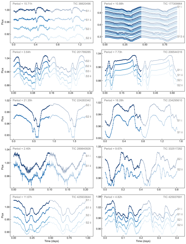
Figure A1: All available TESS light curves of young M dwarfs with complex photometric variability, spanning multiple Sectors of TESS observations. Each light curve shows the data of one TESS orbit (14 days of observations) phase-folded onto the rotational period of each star, with, e.g., ”S1 i” denoting the first orbit of Sector 1 and ”S13 ii” denoting the second orbit of Sector 13. Flares have been removed prior to phase-folding and plotting. All complex rotators’ features show remarkable stability and longevity over many weeks to a year (at least). See also Fig. 8 for a closer view of TIC 17730996.

Most recently, Zhan et al. (2019) discovered ten very similar objects in TESS Sectors 1 & 2,, dubbed complex rotators (Fig. 1 fourth row; see also Fig. A1 for a collage of all light curves per TESS orbit). All complex rotators and scallop shells show rapid rotation, strict periodicity, and dozens of harmonics in their frequency spectra indicating their sharp light curve features. We thus argue that they are likely the same class of objects, and any differences are only due to Kepler’s and TESS’ observing cadences (30 min vs. 2 min). This makes them strictly distinct from ‘normal’ spotted stars (even those with differential rotation), which only show one or two peaks in their frequency spectra, and from dippers, which are far less periodic and morphological stable.

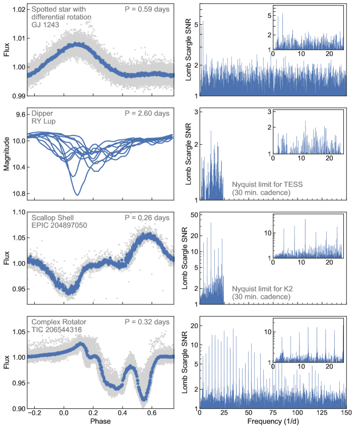
Figure 1: A collage of different morphology classes of young M dwarfs with complex photometric variability. First row: a typical complex rotator (TIC 206544316) with a period of 0.32 days. Its phase-folded light curve highlights the complex modulation, and its frequency spectrum shows dozens of harmonics down to time scales of minutes. Second row: a typical scallop shell (EPIC 204897050) with a period of 0.26 days. It is apparent that these targets share the same morphology class as the complex rotators, even though the data are constrained by the Nyquist limit for K2 (30 min. cadence). Third row: a typical spotted M dwarf with a period of 0.58 days (GJ 1243; see e.g. Davenport et al., 2015, 2020; Günther & Daylan, 2021), showing a simple modulation and only two peaks in the frequency spectrum (two peaks rather than one due to differential rotation). Fourth row: a typical dipper star observed with TESS (RY Lup; Bredall et al., 2020), usually showing no strict periodicity, no presence of multiple clear harmonics, and a wider range of periods (multiple days to weeks). Not shown are the more standard variability classes, such as single spot modulation and binary stars.

1.2 Hypotheses for complex modulations and their limitations

All dipper and burster classes were linked to the presence of dusty disks and a viewing-angle dependency, suggested by observations of strong infrared excess (accreting dust disks; Bodman et al., 2017, Fig. 2 first panel).

The scallop shells were first suggested to arise from a patchy torus of material clouds at the Keplerian co-rotation radius periodically transiting the star (co-rotating clouds; Stauffer et al., 2017, 2018, Fig. 2 second panel). Such material might be warm coronal gas, dust, or a mixture of both.

When studying the complex rotators, however, Zhan et al. (2019) suggested a new idea: spotted, rapidly rotating stars that host an inner dust disk at a few stellar radii, and show a spin-orbit misalignment between their rotation axis and the dust ring (spots and misaligned disk; Fig. 2 third panel). Spots might then pass behind the dust disk and get (partially) occulted, leading to sudden increases in photometric brightness.

In particular, Zhan et al. (2019) presented the following counterarguments to the previous hypotheses:

• Spots only: even the superposition of multiple cold and hot stellar spots leads to smooth variations and can only explain 1–2 peaks in the frequency spectrum (also Kővári & Bartus, 1997; Stauffer et al., 2017).

• Accreting dust disk: (i) complex rotators’ stable periodicity is in stark contrast to the semi-periodic and stochastic nature of morphologies caused by accreting disks; (ii) the absence of significant infrared excess in their spectral energy distributions (SEDs) contradicts the presence of accreting disks; (iii) their roation periods are much shorter than those of dippers (also Stauffer et al., 2017).

• Co-rotating clouds: (i) if the material is gas, it is challenging to explain the large amplitudes of the modulation; (ii) the material cannot be dust, as it cannot be stably confined at the required distances of several stellar radii because the magnetic field at those large distances from the surface would be too weak; (iii) any material (be it gas or dust) trapped in the magnetic field closer to the stellar surface could not reproduce the observations of sharp features with amplitudes of several percent.

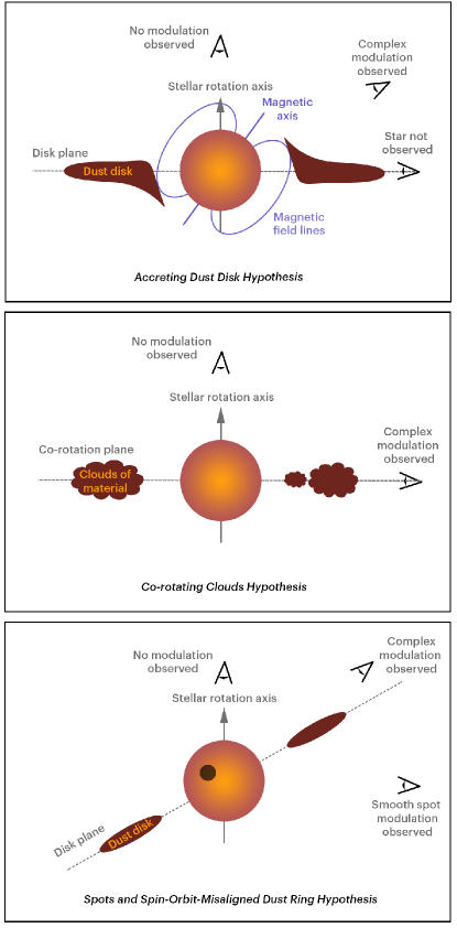
Figure 2: Three hypotheses to explain complex morphologies of young M dwarfs. First panel: Accreting dust disk hypothesis (Bodman et al., 2017), where an accreting dust disk seen from different observing angles could explain dipper and burster stars. Second panel: Co-rotating clouds hypothesis (Stauffer et al., 2017, 2018), where a patchy torus of gas clouds at the Keplerian co-rotation orbit periodically blocks out stellar light and might cause scallop shell modulation. Third panel: Spots and misaligned disk hypothesis (Zhan et al., 2019), where spot occultations might explain the complex rotator’s modulation.

1.3 This paper

This paper focuses on the ten targets discovered by Zhan et al. (2019) to further scrutinize the plausibility of several hypotheses by three means:

1. investigating their occurrence rates,

2. studying the morphologies’ stability and longevity over one (non-continuous) year, and

3. probing the feature’s chromaticity.

We give an overview of all observations in Section 2, and revise the stellar parameters in Section 3. Then, we study stellar flares and other brightenings in Section 4. Next, we scrutinize all hypotheses with respect to occurrence rates, stability and longevity, and color dependency in Section 5. Finally, we discuss our findings and present our conclusion in Sections 6 and 7.

2 Observations

2.1 TESS photometry

The ten complex rotators were discovered in TESS short-cadence data from Sector 1 (2018-07-25 to 2018-08-22) and Sector 2 (2018-08-22 to 2018-09-10) and observed as part of the cool dwarf catalog (Stassun et al., 2018; Muirhead et al., 2018). Here, we also add new data taken over the full first year of operations (Tab. 1). Light curves were prepared with the Science Processing Operations Center (SPOC) pipeline (Jenkins et al., 2016), a descendant of the Kepler mission pipeline (Jenkins, 2002; Jenkins et al., 2010; Jenkins, 2017; Stumpe et al., 2014; Smith et al., 2012). We use the pre-search data conditioned simple aperture (PDC-SAP) light curves, which are detrended for instrumental systematics.

2.2 SPECULOOS Southern Observatory photometry

The SPECULOOS Southern Observatory (SSO; Gillon, 2018; Burdanov et al., 2018; Delrez et al., 2018) is located at ESO’s Paranal Observatory in Chile and is part of the SPECULOOS network. The facility consists of four robotic 1-m telescopes (Callisto, Europa, Ganymede, and Io), each equipped with a near-infrared-sensitive CCD camera with a resolution of 0.35 arcsec per pixel. We observed four targets, TIC 201789285, TIC 206544316, TIC 332517282, and TIC 425933644, each simultaneously in at least two wavelength bands (g’, r’, i’, and z’ band filters) for an entire observing night (Table A1). We extracted light curves using the SSO pipeline (Murray et al., 2020), which uses the casutools software (Irwin et al., 2004) for automated differential photometry and detrends for telluric water vapor.

2.3 ANU spectroscopy

We also reuse the spectroscopic observations taken by Zhan et al. (2019). The low-resolution spectra covered four of the systems (TIC 177309964, TIC 206544316, TIC 234295610, and TIC 425933644) using the Wide Field Spectrograph (WiFeS; Dopita et al., 2007) on the Australian National University (ANU) 2.3 m telescope at Siding Spring Observatory, Australia, on January 18 and 19, 2019. The observations cover the 5200–7000 Å band with a resolving power of $R=7000$ and were reduced following Bayliss et al. (2013). All spectra reveal strong H$\alpha$ emission features with equivalent widths of 4–7 Å, typical of rapidly rotating young M stars (see Section 3). No signs of a binary nature of these four objects were found.

3 Revising the stellar parameters

3.1 Revisiting the binary TIC 289840928 and TIC 289840926

Zhan et al. (2019) found two prominent rotation periods for TIC 289840928, which is in a spatially resolved binary system with TIC 289840926 and both stars are blended in a single TESS pixel. In our re-analysis, the TESS pixel-level data revealed the primary (TIC 289840928, M4V, 3100 K) only has a smooth spot modulation with a period of 15.625 h, while the secondary (TIC 289840926, M6V, 2800 K) is the actual complex rotator with 2.400 h. We thus update all corresponding values here.

3.2 Ages and activity corrections

Zhan et al. (2019) estimated the ages of all ten complex rotators via their probabilistic membership of young stellar associations, using the banyan sigma software (Gagné et al., 2018), with input from the TESS Input Catalog version 8 (TICv8; Stassun et al., 2018) and Gaia Data Release 2 (Gaia DR2 Collaboration et al., 2018). They found that all ten targets have a high probability of belonging to young associations (see Table 1).

We here conduct an independent estimate of their stellar age. Young M dwarfs are pre-main-sequence stars and as such have larger radii than their main-sequence counterparts of the same mass. Additionally, they have high levels of activity, leading to activity induced radius inflation and temperature suppression (Stassun et al., 2012). This could be due to strong chromospheric activity, presumably arising from rapid rotation. We can thus use the ANU spectra of four targets (Section 2.3) to explore if these stars have larger radii than expected for the main-sequence.

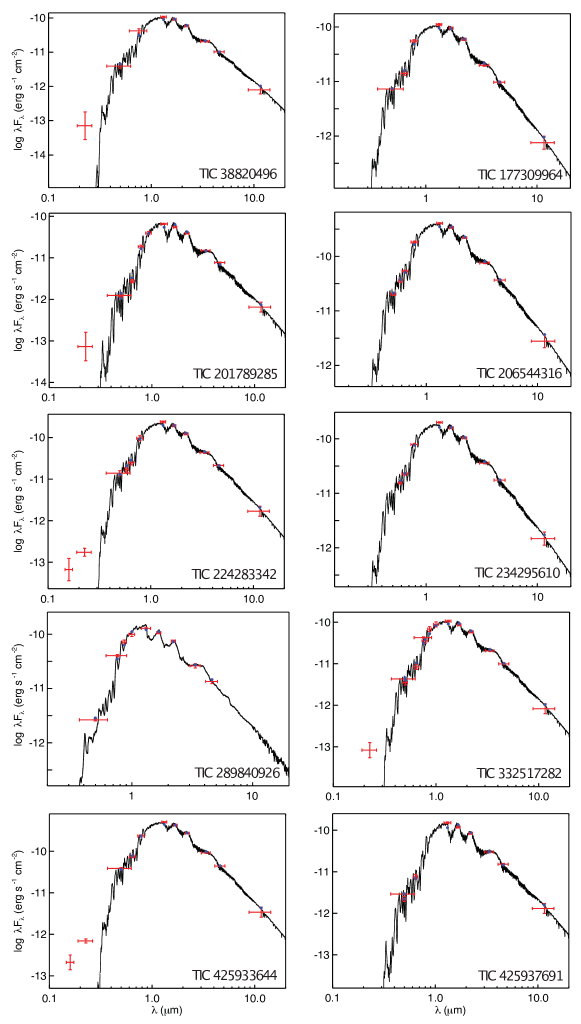
Figure A2: All spectral energy distribution (SED) fits for the ten complex rotators. The results are used to determine the stars’ apparent effective temperatures and radii. The near-UV and blue optical excesses for some targets are consistent with chromospheric activity, another indicator of strong magnetic activity for these stars. Notably, no infrared excesses are seen.

For example, TIC 234295610 shows an H$\alpha$ equivalent width of 6.8 Å in the ANU spectrum. According to the empirical relations from Stassun et al. (2012), this equivalent width (EW) predicts a radius inflation of 15.6% and a temperature suppression of 7.1%. Next, we performed a spectral energy distribution (SED) fit to better constrain the apparent radius to ${R_{\star}^{\mathrm{apparent}}}=0.415\pm 0.029$ $R_{\odot}$ and the apparent temperature to $T_{\mathrm{eff}}^{\mathrm{apparent}}=3075\pm 100$ K (see Fig. A2). Assuming that this radius and temperature represent the activity-inflated radius and activity-suppressed temperature values, then in the absence of activity we would have $R_{\star}^{\mathrm{w/o~{}activity}}\approx 0.36$ $R_{\odot}$ and $T_{\mathrm{eff}}^{\mathrm{w/o~{}activity}}\approx 3300$ K.

Comparing the corrected values with models for low-mass pre-main-sequence stars (Baraffe et al., 2015), we find that they are fully consistent with a star of mass of 0.20 $M_{\odot}$ and age of 40 Myr. This leads to a stellar mass that is only half of the mass of a main-sequence star with the same radius and effective temperature. We consider this a strong affirmation of the young age suspected from its young association membership.

We perform the same revision of stellar parameters for all systems. First, we perform SED fits to refine all their $T_{\mathrm{eff}}^{\mathrm{apparent}}$ and $R_{\star}^{\mathrm{apparent}}$ (see Fig. A2). Next, for those with ANU spectra (TIC 177309964, TIC 206544316, TIC 234295610, and TIC 425933644), we measure their H$\alpha$ EWs and use them to compute the temperature suppression and radius inflation factors, providing the corresponding values ‘without activity’. For the other six targets, we provide provisional corrections assuming they have H$\alpha$ EWs comparable to the average of the four measured ANU spectra.

Fig. 3 and Table 1 summarize the revised stellar parameters and their isochrone matches. The ‘corrected’ $T_{\mathrm{eff}}$ and radii place nine of the ten complex rotators in the range of $\sim$20 or $\sim$50 Myr, consistent with the respective ages of their young associations. Only TIC 332517282 falls closer to the $\sim$150 Myr isochrone, consistent with its membership in AB Doradus (150 Myr), making it our single ‘oldest’ star.

Table 1: Updated parameters of the complex rotators from TESS Sectors 1 & 2.

TIC ID 1	38820496	177309964	201789285	206544316	224283342	234295610	289840926*	332517282	425933644	425937691
RA (deg) 1	7.19516	103.45258	33.88868	18.41884	356.35758	357.98325	317.629044	350.8786	3.69942	5.36556
Dec (deg) 1	-67.86237	-75.70396	-56.45488	-59.65974	-40.33782	-64.79293	-27.18098	-28.12114	-60.06352	-63.85226
Association 2	Tuc. Hor.	Carina	Tuc. Hor.	Tuc. Hor.	Columba	Tuc. Hor.	$\beta$ Pictoris	AB Doradus	Tuc. Hor.	Tuc. Hor.
Membership Probability 2	99.9%	83.2%	99.7%	100.0%	75.0%	99.9%	99.0%	99.1%	99.8%	98.8%
Age (Myr) 2	$45\pm 4$	$45^{+11}_{-7}$	$45\pm 4$	$45\pm 4$	$42^{+6}_{-4}$	$45\pm 4$	$24\pm 3$	$149^{+51}_{-10}$	$45\pm 4$	$45\pm 4$
Distance (pc) 1	$44.06\pm 0.12$	$91.08\pm 0.49$	$45.16\pm 0.17$	$43.07\pm 0.10$	$38.12\pm 0.10$	$48.17\pm 0.11$	$40.33\pm 0.18$	$39.08\pm 0.10$	$44.26\pm 0.18$	-
Rotation Period (h) 3	15.71	10.88	3.64	7.73	21.35	18.28	2.40	9.67	11.67	4.82
H$\alpha$ Equivalent Width (A) 4	(5.3)	5.8	(5.3)	4.8	(5.3)	6.8	(5.3)	(5.3)	3.8	(5.3)
App. Eff. Temp., $T_{\mathrm{eff}}^{\mathrm{app}}$ (K) 5	$3000\pm 100$	$3200\pm 100$	$2800\pm 100$	$3100\pm 100$	$3100\pm 100$	$3100\pm 100$	$2700\pm 100$	$3000\pm 100$	$3200\pm 100$	$2800\pm 100$
App. Radius, $R_{\star}^{\mathrm{app}}$ ($R_{\odot}$) 5	$0.30\pm 0.02$	$0.57\pm 0.04$	$0.27\pm 0.02$	$0.54\pm 0.04$	$0.36\pm 0.02$	$0.42\pm 0.03$	$0.38\pm 0.03$	$0.27\pm 0.02$	$0.59\pm 0.04$	$0.38\pm 0.03$
Temp. Suppression 6	(6.2%)	6.5%	(6.2%)	6%	(6.2%)	7.1%	(6.2%)	(6.2%)	5.3%	(6.2%)
Radius Inflation 6	(13.5%)	14%	(13.5%)	13%	(13.5%)	15.6%	(13.5%)	(13.5%)	11.5%	(13.5%)
Eff. Temp., $T_{\mathrm{eff}}^{\mathrm{w/o~{}act}}$ (K) 6	(3200)	$3400\pm 100$	(3000)	$3300\pm 100$	(3300)	$3300\pm 100$	(2800)	(3200)	$3400\pm 100$	(3000)
Radius, $R_{\star}^{\mathrm{w/o~{}act}}$ ($R_{\odot}$) 6	(0.26)	$0.50\pm 0.04$	(0.24)	$0.48\pm 0.04$	(0.32)	$0.36\pm 0.03$	(0.33)	(0.23)	$0.53\pm 0.04$	(0.33)
Mass, $M_{\star}$ ($M_{\odot}$) 7	(0.15)	0.29	(0.08)	0.22	(0.19)	0.2	(0.08)	(0.16)	0.29	(0.08)
Surface Gravity, $\log_{10}(g)$	(4.7)	4.4	(4.5)	4.3	(4.6)	4.5	(4.2)	(4.8)	4.4	(4.2)
Co-rotation Radius, $R_{\mathrm{cr}}(R_{\star})$	5.6	2.9	1.9	2.2	6.2	4.9	1.0	4.6	2.9	1.6
TESS Sectors	1–2	1–13	2–3	1–2	2	1	1	2	1–2	1–2

Tuc. Hor.: Tucana Horlogium; ¹ from TICv8 (Stassun et al., 2018); ² via Banyan Sigma (Gagné et al., 2018); ³ via TESS photometry; ⁴ via ANU spectroscopy; ⁵ via SED fit; ⁶ via (Stassun et al., 2012); ⁷ via (Baraffe et al., 2015) models for a star with the respective age, $T_{\mathrm{eff}}^{w/o~{}act}$, and $R_{\star}^{w/o~{}act}$; Values in parentheses are only estimated using the mean H_α equivalent width of the other four targets, and should only be used as an approximate guidance. * TIC 289840926 and TIC 289840928 form a binary system that is blended in a single TESS pixel, but is spatially resolved by other surveys. TIC 289840926 is the complex rotator (see Section 3.1).

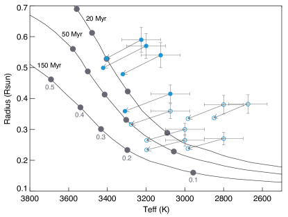
Figure 3: Revised stellar parameters of the ten complex rotators after correcting for activity-induced radius inflation and temperature suppression. Solid curves are isochrones from the Baraffe et al. (2015) models for ages of 20, 50, and 150 Myr, with gray circles marking masses at 0.1 $M_{\odot}$ increments. Error bars show apparent effective temperatures ($T_{\mathrm{eff}}$) and radii measured from SED analyses. Arrows show where the stars would fall if they were inactive, i.e., after they are corrected for activity. Filled blue circles mark the four targets with H$\alpha$ measurements from ANU (Section 2.3), whereas empty blue circles mark the remaining six targets for which we provide estimates only. The ‘corrected’ values place most of the stars near isochrones consistent with the respective ages estimated from their young association memberships, suggesting inferred masses of 0.1–0.3 $M_{\odot}$ (Table 1).

4 Flares and sudden brightenings

The complex rotators and scallop shells show frequent and large-amplitude flaring, along with other sudden brightenings whose shapes are distinct from usual M dwarf flare profiles (Stauffer et al., 2017, 2018; Zhan et al., 2019). In particular, brightenings of the entire modulation often appeared right after strong flares, sometimes even followed by changes in the overall morphology, underlining strong magnetic activity.

It is still disputed whether flares on stars other than our Sun correlate with the rotational phase and are linked to localized clusters of spots on the stellar surface. Many previous studies found that superflares were distributed randomly uniform over the rotational phase for main sequence dwarfs (Roettenbacher & Vida, 2018; Doyle et al., 2018, 2019, 2020), and young stars (Vida et al., 2016; Feinstein et al., 2020b). Doyle et al. (2018) reason that depending on the viewing geometry, polar spots could be seen at all phases, and their interaction with emerging active regions can thus cause continuously visible flaring. However, other studies found flares to be more prominent at certain rotational phases, and hence potentially bound to the locations of star spots for the Sun (Zhang et al., 2008), Sun-like stars (Notsu et al., 2013), and the smallest flares on main sequence dwarfs (Roettenbacher & Vida, 2018). Hence, a unifying idea is that superflares occur over the entire surface while small flares are tied to spots.

Here, we utilize the extended coverage by TESS (up to one year for TIC 177309964) to study whether complex rotators’ flares and other brightenings correlate with the phase of the modulation. We searched the light curves in two ways. In the first approach, we ran the stella software, a convolutional neural network developed for probabilistic flare detection in TESS 2 min. cadence data (Feinstein et al., 2020b, a). As the algorithm was trained on a large sample of stars with smooth spot modulation, many of the initial flare candidates were misidentified (often spikes of the complex rotators). By visually vetting, we then selected reliable criteria of a probability $\geq$0.9 and amplitude $\geq$5%, and identify a confirmed sample of at least 67 flares on TIC 177309964. In the second approach, we independently inspected the entire light curve by eye, and found a total of $\sim$70 confirmed flares, agreeing with the machine learning results.

We find that flares on the complex rotators are distributed randomly uniform in phase, showing no clear dependency of their location or amplitude (see example of TIC 177309964 in Fig. 4). There is also no clear correlation between flare amplitudes and the one year time span. It is peculiar that the three largest flares (amplitudes of 1.5 to 4 in normalized flux) all occur within two few weeks from one another, but the sample size is too low to rule out mere coincidence. Most flares are described by the same profiles as their main sequence counterparts, suggesting similar origins and processes driving them. We also observed somewhat more complicated ‘outbursts’ of flares, which again resemble those of main sequence M dwarfs; these can be explained as superpositions of multiple flare events (e.g. Günther et al., 2020).

Finally, we also find that some sudden brightenings do not resemble typical M dwarf flare profiles (Fig. 5); instead, they seem like amplified versions of the complex periodic morphology. This was also pointed in Zhan et al. (2019) and Stauffer et al. (2017), often (but not always) following superflares. On TIC 177309964, these alterations also occur without any preceding flare observation. It is possible that they were triggered by a superflare that was (i) not visible in the visual, but would have been classified as such in the UV or X-ray spectrum (e.g. Wolter et al., 2007; Loyd et al., 2020), or (ii) was located outside of the visible hemisphere.

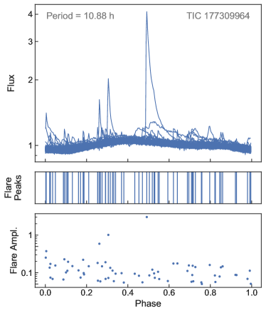
Figure 4: Flares on complex rotators appear randomly uniform distributed in phase, exemplified by one year of TESS data on TIC 177309964. The top panel shows the phase folded light curve with all flares. The middle panel shows the locations of all flare peaks, illustrating the randomly uniform distribution. The bottom panel illustrates that there is no clear correlation between flare amplitude and phase.

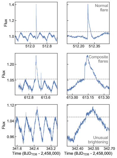
Figure 5: Different flare and brightening profiles of the complex rotators, exemplified by TIC 177309964. Each row shows a global (2 day) and local (5 hr) view of the light curve brightening. Horizontal dashed lines show the typical non-flare maximum flux value. First row: normal flares are described by the same profiles as main sequence M dwarfs, suggesting similar origins and processes driving them. Second row: complicated outbursts of flares also resemble those of main sequence M dwarfs, and can be explained as superpositions of sequential flare events (e.g. Günther et al., 2020). Third row: unusual brightenings in the complex rotators often, but not always, occur after large flares, and show an amplified version of the usual morphology for a short time.

5 Testing the hypotheses

The limitations of previous hypotheses leave us with two remaining possibilities for the complex rotators and scallop shells: (i) the idea of a patchy torus of clouds of gas at the Keplerian co-rotation radius (co-rotating clouds hypothesis) and (ii) the idea of spots being periodically occulted behind a spin-orbit-misaligned dust disk (spots and misaligned disk hypothesis). In the following analyses, we hence focus on these two cases.

5.1 Occurrence rates

We can estimate the expected yield of complex rotators in TESS Sectors 1 & 2 from the co-rotating clouds and spots and misaligned disk hypotheses (see Fig. 2), respectively, as

$$N_{\mathrm{comp.rot.}}^{\mathrm{CC}}=N_{\mathrm{yMrr}}\cdot P_{\mathrm{clouds}}\cdot P_{\mathrm{geom}}$$ (1)

and

$$N_{\mathrm{comp.rot.}}^{\mathrm{SMD}}=N_{\mathrm{yMrr}}\cdot P_{\mathrm{spots}}\cdot P_{\mathrm{disk}}\cdot P_{\mathrm{misal}}\cdot P_{\mathrm{geom}}.$$ (2)

Here, $N_{\mathrm{yMrr}}$ is the number of young M dwarfs with rapid rotations ($\lesssim$ 2 days) which were observed by TESS in short-cadence mode during Sectors 1 & 2. $P_{\mathrm{clouds}}$ is the probability that a given star has a cloud of dust/gas orbiting it at the Keplerian co-rotation radius. $P_{\mathrm{spots}}$ is the probability that a given star has at least one large spot. $P_{\mathrm{disk}}$ is the probability that these stars have a dust disk orbiting them at a few stellar radii. $P_{\mathrm{misal}}$ is the probability that a given star shows a spin-orbit misalignment between the stellar rotation axis and the dust disk. Finally, $P_{\mathrm{geom}}$ is the geometric probability that an existing structure (cloud or disk) falls in the line of sight between the star and the observer.

5.1.1 How many young M dwarfs with rapid rotations are out there?

To first order, we can estimate $N_{\mathrm{yMrr}}$ as the number of stars in known open clusters and associations that have effective temperatures below 3900 K and radii below 0.6 $R_{\odot}$. For this, we cross-match the TESS short cadence target lists of Sectors 1 & 2 with three young star catalogs:

1. a catalog by Feinstein et al. (2020b), which was assembled through a combination of searching the TESS Guest Investigator proposals and the data from Faherty et al. (2018). All targets were vetted with the banyan sigma software (Gagné et al., 2018) and the ones with $\geq 50$% probability and available TESS 2 min data were included.

2. a catalog by Bouma et al. (2019), collecting targets from numerous literature lists, including members of open clusters, moving groups and young associations.

3. a catalog we created by matching all TESS short-cadence targets with the banyan sigma software (Gagné et al., 2018). The algorithm uses a Bayesian model to predict whether a given target is part of one of 27 young associations within 150 parsec. The target is identified by its coordinates, proper motion, parallax, distance, and radial velocity measurements, which we retrieve from TICv8 and Gaia DR2.

The results of our cross-matches are shown in Figure 6. We find a total of 290 young M dwarfs from open clusters and young associations. Notably, their real number might be even higher, as new clusters and associations are still being discovered. For example, Gagné et al. (2020) just discovered a new young association at 150 pc, while Castro-Ginard et al. (2020) recently discovered 582 new open clusters in the Galactic disc using Gaia DR2, increasing their total number by 45% (many beyond 150 pc). Additionally, there might still be unidentified M dwarfs among nearby clusters. We thus consider the number of young M dwarfs in TESS Sectors 1 & 2 as $N_{\mathrm{yM}}\gtrsim 290$.

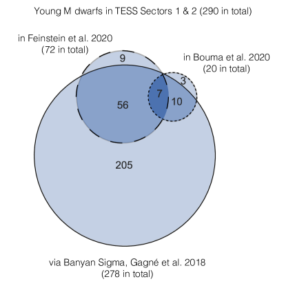
Figure 6: Overlap and union of three young star catalogs cross-matched with the TESS short-cadence targets from Sectors 1 & 2. The three catalogs were assembled by Feinstein et al. (2020b), Bouma et al. (2019), and in this work using banyan sigma (Gagné et al., 2018).

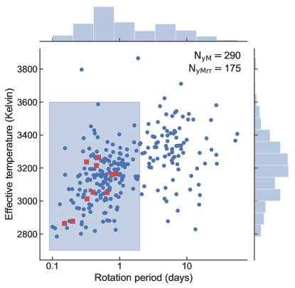
Figure 7: Effective temperatures and rotation periods of the 290 young M dwarf stars in TESS short-cadence from Sectors 1 & 2 (blue circles; $\mathrm{N_{yM}}$: number of young M dwarfs). Out of these, 175 targets show rotation periods shorter than 2 days (blue shaded area; $\mathrm{N_{yMrr}}$: number of young M dwarfs with rapid rotations), comparable to the ten known complex rotators from this sample (red squares).

To estimate $N_{\mathrm{yMrr}}$ from this, we investigate the rotation periods of those 290 M dwarfs using all available TESS data from Sectors 1 through 13. We flag a target as a ‘young M dwarf with rapid rotation’ if we find a rotation period below 2 days using Lomb-Scargle periodograms (Lomb, 1976; Scargle, 1982). We measure rotation periods for 269 out of the 290 targets, with the remaining 21 targets not showing measurable photometric variability (false alarm probability $>$ 0.01). This might just be due to low signal-to-noise, or the stars might simply be seen pole-on; both leaves open that they could actually be rapidly rotating. All measured rotation periods and effective temperatures are shown in Fig. 7, and we conclude that $N_{\mathrm{yMrr}}\gtrsim$ 175.

5.1.2 How many complex rotators should we expect?

We here put the finding of $N_{\mathrm{yMrr}}\gtrsim$ 175 into the perspectives of Eqs. 1 and 2.

Co-rotating clouds hypothesis

For this hypothesis, we also have to account for (i) $P_{\mathrm{clouds}}$, the probability of clouds of dust/gas being present at the Keplerian co-rotation radius, $R_{\mathrm{cr}}$, as well as (ii) $P_{\mathrm{geom}}^{\mathrm{CC}}$ the geometric alignment probability of an edge-on alignment to the observer. We can estimate $P_{\mathrm{geom}}^{\mathrm{CC}}\approx(R_{\star}/R_{\mathrm{cr}})$, with $R_{\mathrm{cr}}$ derived as:

$$R_{\mathrm{cr}}=\left(\frac{P_{\mathrm{rot}}}{2\pi}\right)^{\frac{2}{3}}\left(GM_{\star}\right)^{\frac{1}{3}},$$ (3)

with the rotation period $P_{\mathrm{rot}}$, gravitational constant $G$ and stellar mass $M_{\star}$. For our targets, this yields $R_{\mathrm{cr}}\approx 1-6\,R_{\star}$ (Table 1), which leads to $P_{\mathrm{geom}}^{\mathrm{CC}}\approx(R_{\star}/R_{\mathrm{cr}})\approx 0.2-1$. Putting all pieces together, we can estimate from Eq. 1:

$$\begin{split}N_{\mathrm{comp.rot.}}^{\mathrm{CC}}&=N_{\mathrm{yMrr}}\cdot P_{\mathrm{clouds}}\cdot P_{\mathrm{geom}}^{\mathrm{CC}}\\ &\approx 175\cdot P_{\mathrm{clouds}}\cdot(0.2-1)\\ &\approx(35-175)\cdot P_{\mathrm{clouds}}.\end{split}$$ (4)

Given that we found 10 complex rotators in Sectors 1 & 2, this would only require $\lesssim 30$% of all rapidly rotating young M dwarf to have material clouds trapped at their Keplerian co-rotation radius.

Spots and misaligned disk hypothesis

For this hypothesis, we already searched all known young stars in TESS Sectors 1 & 2 for photometric rotation periods and signs of spots, and found that, on average, $P_{\mathrm{spots}}\sim 1$ (see above). We estimate the geometric probability $P_{\mathrm{geom}}^{\mathrm{SMD}}\approx(R_{\star}/d)$, where $R_{\star}$ is the stellar radius and $d\approx 5-15\,R_{\star}$ is the outer edge (or gap) of a possible disk (Zhan et al., 2019). This leads to $P_{\mathrm{geom}}^{\mathrm{SMD}}\approx 0.07-0.2$ and:

$$\begin{split}N_{\mathrm{comp.rot.}}^{\mathrm{SMD}}&=N_{\mathrm{yMrr}}\cdot P_{\mathrm{spots}}\cdot P_{\mathrm{disk}}\cdot P_{\mathrm{misal}}\cdot P_{\mathrm{geom}}^{\mathrm{SMD}}\\ &\approx 175\cdot 1\cdot P_{\mathrm{disk}}\cdot P_{\mathrm{misal}}\cdot(0.07-0.2)\\ &\approx(12-35)\cdot P_{\mathrm{disk}}\cdot P_{\mathrm{misal}}\end{split}$$ (5)

Considering our 10 complex rotators in Sectors 1 & 2, this would imply that $P_{\mathrm{disk}}\cdot P_{\mathrm{misal}}$ is on the order of $0.3-1$. Hence, for this hypothesis to hold true, a large fraction of $\gtrsim 30$% of rapidly rotating young M dwarfs would need to have an inner dust disk with a slight spin-orbit misalignment to their rotation axis.

5.2 Time dependency

The photometric modulations of the complex rotators appear stable over timescales of at least one year (Fig. 8 and Fig. 9). The complex rotator TIC 177309964 fell into TESS’ continuous viewing zone and was observed for the consecutive Sectors 1–13, spanning an entire year of data from July 2018 until July 2019 (Fig. 8).

We can also see this stability on the examples of TIC 201789285, TIC 206544316, TIC 332517282, and TIC 425933644 (Fig. 9) when combining TESS and SSO photometry. The original TESS data were taken in Aug-Oct 2018, while the SSO observations were taken in Nov/Dec 2019, over one year later. Despite the large time span, the modulation profiles still follow the same pattern and periodicity. All major features remain the same, while only some minor evolution of the morphology is evident in the SSO light curves compared to TESS. In the case of TIC 201789285, it appears that a minor feature has increased in amplitude (near $\mathrm{BJD_{TDB}}$ 2,458,795.70), while another has decreased in amplitude (near $\mathrm{BJD_{TDB}}$ 2,458,795.75).

The stability and longevity of these morphologies is extraordinary. Considering the spots and misaligned disk hypothesis, this is well compatible with the life times of dust disks and the persistence of stellar spots on young M dwarfs. While stellar spots on most stars only last for a few weeks (e.g., on the Sun they last only for 3–6 rotations Gaizauskas et al. 1983), we have examples like GJ 1243, which had remarkably constant spot modulation over 10 years observed with Kepler and TESS (Davenport et al., 2020). Notably, GJ 1243 is a member of a young association with an age of around 30–50 Myr and, as such, quite comparable to our complex rotators. Furthermore, a 200-day photometric monitoring campaign of the open cluster Blanco 1 ($\sim$115 Myr) with the Next Generation Transit Survey (NGTS) suggests that most young M dwarfs display generally stable spot modulation patterns over this baseline, while F, G and early-K dwarfs show moderate-to-significant evolution in their light curve morphologies (Gillen et al., 2020).

In contrast, considering the co-rotating clouds hypothesis, such a stability and longevity would seem surprising. The idea does suggest a rather fine-tuning problem with clouds being confined strictly at the co-rotation radius. Any separating clouds would slowly drift away and slightly alter their orbital period. Even for small drifts, a year-long time-span might lead to noticeable changes in the morphologies. This would lead to a certain amount of material away from co-rotation at any given time, which would blur out the strictly periodic signals over year-long time spans.

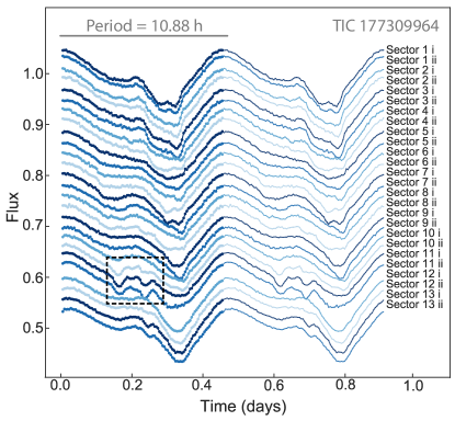
Figure 8: Example of TIC 177309964, illustrating the stability of major photometric features over year-long timescales (TESS orbits from Sectors 1–13, from July 2018 until July 2019). Each orbit is phase-folded to show two periods of the modulation and vertically offset for clarity. Flares have been clipped before plotting. The major features of the modulation remain stable over the full year, while minor features appear and disappear over a few weeks (dashed box).

5.3 Color dependency

We obtained a total of nine telescope nights worth of SSO observations (Section 2.2) to capture four of the complex rotators in simultaneous multi-color bandpasses. We compare all these light curves with phase-folded TESS observations (taken one year earlier) in Fig. 9. Evidently, the sharp-peaked features are more prominent in bluer bandpasses, and less expressed in the reddest bandpasses. This matches the expectations from both the co-rotating clouds and spots and misaligned disk hypotheses: (i) for the co-rotating clouds hypothesis, the material’s extinction would have to be stronger in the blue, leading to deeper features. (ii) for the spots and misaligned disk hypothesis, the contrast between the stellar surface ($\sim$3000 K) and a cool spot is stronger in bluer wavelengths. The disk material could be a gray absorber or could have a color dependency, which would add a secondary effect.

Combining TESS data with SSO r, i and g band observations, our total data span more than one year. We find that the same features are still present in the data at the predicted phases (accounting for uncertainties in the period estimation). There is no doubt that the modulation is still the same, and thus stable and long-lived over year-long time spans.

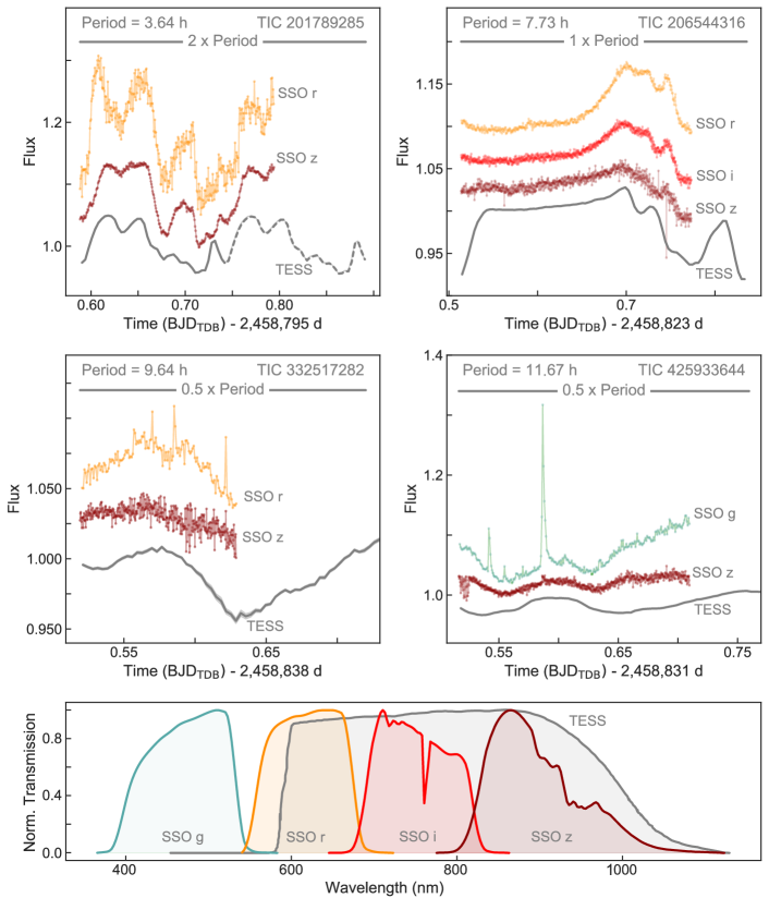
Figure 9: Comparison of multi-color light curves of four of the ten complex rotators: TIC 201789285, TIC 206544316, TIC 332517282, and TIC 425933644. For each target, SSO observations were taken simultaneously in at least two of the g’, r’, i’, and z’ bandpasses (shown as green, orange, red and dark-red curves, respectively). For TESS observations, flares have been removed, and light curves are averaged over all available Sectors, binned in 5 min intervals, and slightly shifted in phase to correct for imprecision in the period measurement (shown as dark-gray curves). The lower panel compares the normalized transmission functions of all respective bandpasses. There is a clear color dependency of the light curve features visible in the simultaneous SSO observations, with features being much more prominent in bluer bandpasses. Additionally, the general shape and largest features in the SSO light curves are still comparable to the TESS light curve, even though the SSO data were taken about 1 year later. This suggests that the overall mechanism causing these patterns also causes a color-dependency (e.g., spots, non-gray dust, or pulsations), and that it is stable over long times.

6 Discussion

6.1 Could spots and pulsations be another hypothesis?

Pulsations on low mass stars have long been theoretically explored and predicted (e.g., Gabriel, 1964; Noels et al., 1974; Palla & Baraffe, 2005; Rodríguez-López et al., 2012, 2014; Rodríguez-López, 2019) but, despite observational efforts, have so far proven elusive. In theory, fully non-adiabatic models of M dwarfs suggest that they could excite (i) radial modes, (ii) low-order, low-degree non-radial modes, and (iii) solar-like oscillations (Rodríguez-López et al., 2012, 2014). This requires the models to be completely convective or have large convective envelopes. This would match the spectral types of all complex rotators and scallop shells, placing the stars beyond the fully convective limit. Periods of the pulsations are predicted to range from 20 min to 3 h, again agreeing with the typical time scales we see for the sharp-peaked features of our targets.

However, the amplitudes of M dwarf pulsations are expected to be in the range of 1 ppm to 1 ppt, while our targets typically show amplitudes of several percent. The only bypass to this caveat could be a superposition of the effects from spots (creating the smooth, large-amplitude modulations) and synchronous pulsations (creating the sharp-peaked, lower-amplitude features). Yet, this would require spots and pulsations to be synchronized, which seems implausible.

Rodríguez-López et al. (2014) identified the theoretical instability strips of M dwarfs, which resulted in two islands of ‘instability’ in the parameter space. Stars falling into one of these islands would, in theory, be capable of showing pulsations. With the revised and activity-corrected stellar parameters (Section 3), some of the stars fall near the lower island, yet remain outside of it. Again, this makes pulsations seem implausible.

6.2 The pros and cons of various hypotheses: a summary

We here briefly summarize the pros and cons of the various hypotheses introduced and scrutinized throughout this paper (see Sections 1 and 6.1 for short overviews). Fig. 10 additionally contrasts all observations with all hypotheses, highlighting which aspects can and cannot be explained through a given hypothesis.

Spots only

Pro: Spot modulations can be strictly periodic and stable over many years, even in the presence of differential rotation (e.g., Davenport et al., 2020). The temperature difference between the surface and the spots causes a color dependence, and spots would not cause any infrared excess. Most young stars are spotted and are often accompanied by strong signs of magnetic activity, such as flaring. Con: Spots alone cannot explain the sharp-peaked features (Zhan et al., 2019). However, spots could still play a major role in combination with other factors (e.g, pulsation or circumstellar material; Sections 6.1 and 6.3).

Accreting dust disk

Pro: Accreting dust disks can lead to the morphologies for dipper/burster stars and occur frequently enough. They might show color dependency depending on the absorption and scattering properties of the material. Con: Accretion is a rather stochastic process, and thus neither strictly periodic nor stable. The dippers and bursters also show strong infrared excess due to the large disks.

Co-rotating clouds of material

Pro: Clouds of material at the Keplerian co-rotation radius could qualitatively explain sharp features and strict periodicity (Stauffer et al., 2017, 2018). Depending on the material, a color dependency is possible, and small enough clouds would cause no infrared excess. As young stars are often surrounded by material, they could also occur at high enough rates. Con: If the material is gas, the absorption would likely not be able to explain percentage-scale amplitudes (Zhan et al., 2019). If the material is dust, these clouds are likely not stable at the required distances ($d/R_{\star}\gtrsim 3$; Zhan et al. 2019). Another challenge might be the stability and longevity of the morphology over year-long time spans, i.e., over hundreds of orbital periods. With some parts of the clouds slowly drifting away from co-rotation, the signals would blur out and evolve, which does not seem to be the case.

Material trapped near the surface

Pro: Material trapped in the magnetic field and bound to the stellar rotation would remain strictly periodic, and could survive over many years near the stellar surface ($d/R_{\star}\sim 1$; Zhan et al. 2019). Depending on the material’s properties, a color dependence is possible, and in small amounts it might not cause any infrared excess. Con: Any material that close in cannot explain the sharp-peaked, percentage-scale amplitudes of the modulation but would instead produce a rather smooth variation similar to spots; this can only be explained by material at larger distances ($d/R_{\star}\gtrsim 3$; Zhan et al. 2019).

Spots and spin-orbit-misaligned dust disks

Pro: The patterns can be strictly periodic and stable over many years. Spots induce a color dependency, and disk material might add to this effect. There are enough young and rapidly rotating M dwarfs in the sample to explain the high occurrence rates (with caveats, see below). Lastly, the spots are a sign of magnetic activity, and agree with the frequent flaring found on the complex rotators and scallop shells. Con: the scenario would require most young M dwarfs to have close-in dust disks with spin-orbit misalignments. There is no obvious formation mechanism that would explain this behavior. Also, the one M dwarf for which we have disk and rotation measurements, Au Mic, does appear co-planar. However, the misalignment does not need not to be very large. A 10^∘ obliquity between the spin and magnetic axes of T Tauri stars is reasonable, based on Zeeman studies and recent work by McGinnis et al. (2020). If the disks are confined by the magnetic field, this slight misalignment could already be enough to mitigate this caveat and cause the observed morphologies. A potential driver for such misalignment might be perturbations from nearby passing stars, either dynamically or through radiation pressure (e.g. Rosotti et al., 2014).

Spots and pulsations

Pro: In theory (qualitatively), a superposition of spots and pulsations could lead to a smooth large-amplitude trend (due to spots) superposed by a sharp-peaked small-amplitude pattern (due to pulsations). Both features can be stable over long times, show color dependencies, a lack of infrared excess, and frequent flaring due to their activity. Con: This would require a strict synchronization between rotation and pulsation, which seems implausible. Further, the stars do not lie within any of the theoretical instability islands.

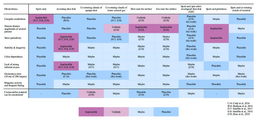
Figure 10: Overview of hypotheses discussed throughout this paper for complex rotators (and scallop shells). All hypotheses are contrasted against observational constraints.

6.3 Towards a unified hypothesis: could it be spots and co-rotating clouds of material?

So far, none of the hypotheses stand out as a definite answer, and each come with limitations. The two most promising hypotheses have their own caveats. On the one hand, the co-rotating clouds hypothesis, with clouds of gas at the Keplerian co-rotation radius could remain stable and allow the required viewing angle, but gas likely cannot explain the large, percentage-scale absorption features. On the other hand, the spots and misaligned disk hypothesis could tick all boxes, but has the implicit requirement that a large fraction of rapidly rotating young M dwarfs must have misaligned disks. That said, if the disks are confined by the magnetic field, a small misalignment of $\sim$10^∘ seems not to be uncommon (McGinnis et al., 2020) and could have been induced by nearby passing stars (e.g. Rosotti et al., 2014).

Rapidly rotating young M dwarfs are known to be magnetically active and generally show high spot coverage rates. Spots alone were ruled out easily, but what was not explored so far is: how much can spots explain?

The superposition of smooth, large-amplitude spot modulations and sharp, sudden features from transits of co-rotating clouds of gas could represent a unified hypothesis (Spots and co-rotating clouds). This explanation could expand the co-rotating clouds hypothesis by requiring only a minimal amount of circumstellar material to cause the overall morphology, making gas clouds a more plausible candidate. It would also mitigate the occurrence rate caveats which challenge the spots and misaligned disk hypothesis.

6.4 Toy models

We developed simplified forward models for the three most promising ideas, the (i) co-rotating clouds, (ii) spots and misaligned disk, and (iii) spots and co-rotating clouds hypotheses. We took the TESS light curve of TIC 201789285 as an example, and tried to imitate its morphology as closely as possible while keeping the models simple, using a hybrid of statistical inference and manual parameter selection. We model the star as a fine grid in spherical coordinates. The rotation axis of the star is left as a free parameter, and a quadratic limb darkening effect is applied to each cell based on its orientation relative to the observer.

For the spots and misaligned disk hypothesis, we model spots with four parameters: two angles describing the location on the star, its size, and its temperature. The disk is parametrized by its inner and outer radius, inclination, and opacity. The observed flux is computed for each grid cell by integrating the Planck function across the TESS bandpass, accounting for geometric effects, spots and the disk. We then try to mimic the TESS light curve of TIC 201789285 by choosing a simple model with three cold spots and a fully opaque disk, optimizing their parameters using nested sampling via dynesty (Speagle, 2020).

For the co-rotating clouds and spots and co-rotating clouds hypotheses, we model the torus of clouds as a series of orbiting spheres whose orbital period matches the rotational period of the star. For this, we used the processing package (https://processing.org/) to draw the model and count the flux in each pixel. We then manually evaluated different scenarios of spots and sparse to dense tori of clouds.

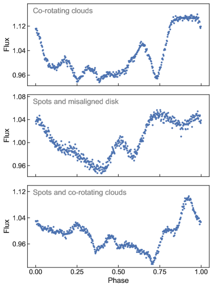
Figure A3: Toy models of a complex rotator derived from three different hypotheses, aiming to replicate the morphology of TIC 201789285.

We find that all three toy models can replicate the typical morphology of complex rotators (Fig. A3). Additionally, spots as drivers for an underlying large-amplitude modulation can explain a large portion of the signal, easing the constraints on circumstellar material.

6.5 What can TESS short-cadence do for us?

The TESS complex rotators were all found in short-cadence (2 min) observations. In contrast, the K2 scallop shells were discovered using 30 min cadence. However, the longer cadence means that the data are limited by the Nyquist frequency, and numerous harmonics will be missed in the frequency spectrum (see Fig. 1). We tested whether we would have discovered the complex rotators in the same way from TESS long-cadence (30 min) observations, by extracting light curves directly from the full frame images (FFI). For this, we used a TESS FFI photometry pipeline based on the one developed by Pál (2012). It is designed to extract photometry of faint stars in crowded fields (TESS-mag$>$15) by combining difference and aperture photometry. We selected nearby stars from the Gaia DR2 catalog that could contaminate the target’s light curve and applied a principle component analysis (PCA) detrending.

We find that the complex rotators morphologies are most apparent in the 2 min cadence data, and that many might have been missed due to their sharp-peaked features being blurred out in 30 min cadence data (Fig. 11). The 2 min data will thus be the best source to search for more complex rotators throughout Sectors 1–23. With the start of the TESS extended mission, 20 s cadence data will be enabled. Additionally, both the original TESS sectors as well as the K2 fields will be revisited. Re-observing complex rotators and scallop shells with such short cadence could greatly increase our sensitivity to the sharpest features.

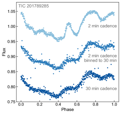
Figure 11: Comparison of TESS 2 min and 30 min light curves on the example of TIC 201789285, showing that the complex rotators’ sharp-peaked features are blurred in long-cadence data. TESS’ 2 min and upcoming 20 s observing cadences are hence ideal for detecting more of these targets.

6.6 Implications for exoplanet systems

We know thanks to Kepler and other missions that, in average, each early- to mid-M dwarf has at least one small exoplanet (Dressing & Charbonneau, 2015). All complex rotators and scallop shells are young mid-M dwarfs (most around 10 – 45 Myr), raising the question of how the effects causing their morphology might impact young, recently formed exoplanets. After all, for the co-rotating clouds, spots and misaligned disk, and spots and co-rotating clouds hypotheses, occurrence rates suggest that most young M dwarfs would go through the same processes, we just cannot see their morphologies (Section 5.1).

At these ages, most processes driving planet formation have likely been concluded. Terrestrial planet formation is thought to be completed after at most 10–30 Myr, regardless of the driving processes (e.g., Chambers, 2010). Particularly, gas giant planets around mid- to late M dwarfs are rare; even if they formed around any complex rotators, they require a substantial amount of gas in the proto-planetary disk to be present at the late stage of their formation, yielding formation time spans of less than 10 Myr (the maximal lifetime of gas discs; e.g., D’Angelo et al. 2010).

The material in question for causing the complex morphologies, however, is likely much closer to the star (near 3–10 stellar radii) than any forming or migrating exoplanets. Exoplanet systems hosted by mid-M dwarfs are widely studied, and if the effects at play for complex rotators are indeed ubiquitous at early ages, they seem to not have caused a strong effect on their planets.

If the spots and misaligned disk hypothesis were correct, more than half of all young M dwarfs would have a slight spin-orbit misalignment between their rotation axis and remnant dust disk. An interesting question is whether this would imply the proto-planetary disk to also be misaligned. However, there are currently no strong signs that a large fraction of exoplanets forming around M dwarfs have spin-orbit misalignments. Limited data suggest there to be a wide variety. For example, Au Mic b is proven to be aligned (e.g, Hirano et al., 2020a), the TRAPPIST-1 system might be slightly misaligned (Hirano et al., 2020b) and GJ 436 b is inclined (Knutson et al., 2011; Bourrier et al., 2017).

7 Conclusion

Recently, at least one new distinct morphology class of young stars has been discovered in white-light photometry from Kepler/K2 and TESS (Stauffer et al., 2016, 2017; Zhan et al., 2019), adding to the seven classes established by Cody et al. (2014) (which include dippers and bursters). Here, we added three puzzle pieces to unveil the physical nature of these complex rotators and probe whether several hypotheses could hold true given these new observational constraints.

The tested hypotheses include spots only, accreting dust disks, co-rotating clouds of material, magnetically constrained material, spots and a spin-orbit-misaligned disk, and spots and pulsations. We particularly focused on the co-rotating clouds and spots and misaligned disk hypotheses, as others are ruled out more easily.

First, we investigated if their occurrence rates make sense in the light of the total number of rapidly rotating young M dwarfs in the given field of view. We find that TESS Sectors 1 & 2 harbor at least 175 young M dwarfs with rotation periods below 2 days, rendering the finding of 10 complex rotators plausible. However, for both hypotheses this comes with a caveat. For the co-rotating clouds hypothesis to work, this would mean that almost every such star must have clouds of dust/gas trapped at the Keplerian co-rotation radius. For the spots and misaligned disk hypothesis to work, this would imply that a large fraction of these stars must have an inner disk and show a spin-orbit-misalignment. If the latter held true, it could have consequences for exoplanet systems around mid-to-late M dwarfs, which might have formed under the same conditions.

Second, we studied the longevity of these features over one year, and find that they remain remarkably stable over these time spans. While the major features of the complex rotators remain unchanged, we find evidence for additional small features building up and decaying over a few weeks. In the Co-rotating Clouds hypothesis, this would imply subtle changes in the dust/gas cloud structures. In the Spots and Misaligned Disks hypothesis, this can very likely be caused by smaller spots appearing and disappearing, major spots changing size, or spots wandering along the surface.

Third, we probe the color-dependency of the complex rotators photometric features. We indeed find the expected behavior predicted by both the co-rotating clouds and spots and misaligned disk hypotheses. The features are more pronounced in bluer wavelengths, which could be explained by either chromatic absorption by the circumstellar material or the smaller spot-to-star brightness contrast in the red / infrared.

All new clues to the case – occurrence rates, longevity and color-dependency – could in principle match any of the hypotheses shown in Fig. 2. It is well possible that the truth will lie somewhere between these hypotheses. Rapidly rotating young M dwarfs are known to be magnetically active, so the final answer will likely have contributions from both spots and circumstellar material, leading to their complex photometric morphologies.

Appendix

Target	Telescope	Date	Filter	Exposure (s)	On sky duration (h)	# images
TIC 201789285	SSO/Io	20191107	r’	35	4.93	392
	SSO/Europa	20191107	z’	40	4.94	357
TIC 206544316	SSO/Io	20191205	z’	10	6.23	1096
	SSO/Europa	20191205	i’	10	6.23	1101
	SSO/Ganymede	20191205	r’	30	6.22	560
TIC 332517282	SSO/Io	20191220	r’	60	2.60	135
	SSO/Europa	20191220	z’	12	2.63	431
TIC 425933644	SSO/Callisto	20191213	g’	50	4.62	278
	SSO/Europa	20191213	z’	10	4.64	827

Table A1: Summary of all SSO observations for four of the ten complex rotators.

References

- Alencar et al. (2010) Alencar, S. H., Teixeira, P. S., Guimarães, M. M., et al. 2010, A&A, 519, doi: 10.1051/0004-6361/201014184
- Ansdell et al. (2016) Ansdell, M., Gaidos, E., Williams, J. P., et al. 2016, MNRAS, 462, 101, doi: 10.1093/mnrasl/slw140
- Baraffe et al. (2015) Baraffe, I., Homeier, D., Allard, F., & Chabrier, G. 2015, A&A, 577, A42, doi: 10.1051/0004-6361/201425481
- Bayliss et al. (2013) Bayliss, D., Zhou, G., Penev, K., et al. 2013, AJ, 146, 113, doi: 10.1088/0004-6256/146/5/113
- Benz & Güdel (2010) Benz, A. O., & Güdel, M. 2010, ARA&A, 48, 241, doi: 10.1146/annurev-astro-082708-101757
- Bodman et al. (2017) Bodman, E. H., Quillen, A. C., Ansdell, M., et al. 2017, MNRAS, 470, 202, doi: 10.1093/MNRAS/STX1034
- Bouma et al. (2019) Bouma, L. G., Hartman, J. D., Bhatti, W., Winn, J. N., & Bakos, G. A. 2019, ApJSS, 245, 13, doi: 10.3847/1538-4365/ab4a7e
- Bouma et al. (2020) Bouma, L. G., Winn, J. N., Ricker, G. R., et al. 2020, AJ, 160, 86, doi: 10.3847/1538-3881/ab9e73
- Bourrier et al. (2017) Bourrier, V., Lovis, C., Beust, H., et al. 2017, Nature, 553, 477, doi: 10.1038/nature24677
- Bredall et al. (2020) Bredall, J. W., Shappee, B. J., Gaidos, E., et al. 2020, MNRAS, 496, 3257, doi: 10.1093/mnras/staa1588
- Browning (2008) Browning, M. K. 2008, ApJ, 676, 1262, doi: 10.1086/527432
- Burdanov et al. (2018) Burdanov, A., Delrez, L., Gillon, M., & Jehin, E. 2018, in Handbook of Exoplanets, ed. H. J. Deeg & J. A. Belmonte (Cham: Springer International Publishing), 1007–1023, doi: 10.1007/978-3-319-55333-7_130
- Castro-Ginard et al. (2020) Castro-Ginard, A., Jordi, C., Luri, X., et al. 2020, A&A, 635, A45, doi: 10.1051/0004-6361/201937386
- Chambers (2010) Chambers, J. 2010, in Exoplanets, ed. S. Seager (University of Arizona Press), 297–317
- Cody et al. (2014) Cody, A. M., Stauffer, J., Baglin, A., et al. 2014, AJ, 147, 2014, doi: 10.1088/0004-6256/147/4/82
- Collaboration et al. (2018) Collaboration, G., Brown, A. G. A., Vallenari, A., et al. 2018, A&A, 616, A1, doi: 10.1051/0004-6361/201833051
- D’Angelo et al. (2010) D’Angelo, G., Durisen, R. H., & Lissauer, J. J. 2010, in Exoplanets, ed. S. Seager (University of Arizona Press), 319–346
- Davenport et al. (2015) Davenport, J. R. A., Hebb, L., & Hawley, S. L. 2015, ApJ, 806, 212, doi: 10.1088/0004-637X/806/2/212
- Davenport et al. (2020) Davenport, J. R. A., Mendoza, G. T., & Hawley, S. L. 2020, AJ, 160, 36, doi: 10.3847/1538-3881/ab9536
- Delrez et al. (2018) Delrez, L., Gillon, M., Queloz, D., et al. 2018, Proc. SPIE, 10700, 107001I, doi: 10.1117/12.2312475
- Dopita et al. (2007) Dopita, M., Hart, J., McGregor, P., et al. 2007, Astrophysics and Space Science, 310, 255, doi: 10.1007/s10509-007-9510-z
- Doyle et al. (2018) Doyle, J. G., Shetye, J., Antonova, A. E., et al. 2018, MNRAS, 475, 2842, doi: 10.1093/mnras/sty032
- Doyle et al. (2020) Doyle, L., Ramsay, G., & Doyle, J. G. 2020, MNRAS, 494, 3596, doi: 10.1093/mnras/staa923
- Doyle et al. (2019) Doyle, L., Ramsay, G., Doyle, J. G., & Wu, K. 2019, MNRAS, 489, 437, doi: 10.1093/mnras/stz2205
- Dressing & Charbonneau (2015) Dressing, C. D., & Charbonneau, D. 2015, ApJ, 807, 45, doi: 10.1088/0004-637X/807/1/45
- Faherty et al. (2018) Faherty, J. K., Bochanski, J. J., Gagné, J., et al. 2018, ApJ, 863, 91, doi: 10.3847/1538-4357/aac76e
- Feinstein et al. (2020a) Feinstein, A., Montet, B., & Ansdell, M. 2020a, JOSS, 5, 2347, doi: 10.21105/joss.02347
- Feinstein et al. (2020b) Feinstein, A. D., Montet, B. T., Ansdell, M., et al. 2020b, AJ, 160, 219, doi: 10.3847/1538-3881/abac0a
- Gabriel (1964) Gabriel, M. 1964, AnAp, 27, 141. https://ui.adsabs.harvard.edu/abs/1964AnAp...27..141G/abstract
- Gagné et al. (2020) Gagné, J., David, T. J., Mamajek, E. E., et al. 2020, ApJ, 903, 96, doi: 10.3847/1538-4357/ABB77E
- Gagné et al. (2018) Gagné, J., Mamajek, E. E., Malo, L., et al. 2018, ApJ, 856, 23, doi: 10.3847/1538-4357/aaae09
- Gaizauskas et al. (1983) Gaizauskas, V., Harvey, K. L., Harvey, J. W., & Zwaan, C. 1983, ApJ, 265, 1056, doi: 10.1086/160747
- Gillen et al. (2020) Gillen, E., Briegal, J. T., Hodgkin, S. T., et al. 2020, MNRAS, 492, 1008, doi: 10.1093/mnras/stz3251
- Gillon (2018) Gillon, M. 2018, Nature Astronomy, 2, 344, doi: 10.1038/s41550-018-0443-y
- Günther & Daylan (2021) Günther, M. N., & Daylan, T. 2021, ApJSS, 254, 13, doi: 10.3847/1538-4365/abe70e
- Günther et al. (2020) Günther, M. N., Zhan, Z., Seager, S., et al. 2020, AJ, 159, 60, doi: 10.3847/1538-3881/ab5d3a
- Hirano et al. (2020a) Hirano, T., Gaidos, E., Winn, J. N., et al. 2020a, ApJL, 890, L27, doi: 10.3847/2041-8213/ab74dc
- Hirano et al. (2020b) Hirano, T., Krishnamurthy, V., Gaidos, E., et al. 2020b, ApJL, 899, L13, doi: 10.3847/2041-8213/aba6eb
- Hunter (2007) Hunter, J. D. 2007, CSE, 9, 90, doi: 10.1109/MCSE.2007.55
- Irwin et al. (2004) Irwin, M. J., Lewis, J., Hodgkin, S., et al. 2004, in Proc. SPIE, Vol. 5493, Optimizing Scientific Return for Astronomy through Information Technologies, ed. P. J. Quinn & A. Bridger, 411–422, doi: 10.1117/12.551449
- Jenkins (2002) Jenkins, J. M. 2002, ApJ, 575, 493, doi: 10.1086/341136
- Jenkins (2017) —. 2017, Kepler Data Processing Handbook
- Jenkins et al. (2010) Jenkins, J. M., Chandrasekaran, H., McCauliff, S. D., et al. 2010, in Proc. SPIE, Vol. 7740, Software and Cyberinfrastructure for Astronomy, 77400D, doi: 10.1117/12.856764
- Jenkins et al. (2016) Jenkins, J. M., Twicken, J. D., McCauliff, S., et al. 2016, in Proc. SPIE, Vol. 9913, Software and Cyberinfrastructure for Astronomy IV, 99133E, doi: 10.1117/12.2233418
- Knutson et al. (2011) Knutson, H. A., Madhusudhan, N., Cowan, N. B., et al. 2011, ApJ, 735, 27, doi: 10.1088/0004-637X/735/1/27
- Kővári & Bartus (1997) Kővári, Z., & Bartus, J. 1997, A&A, 323, 801. https://ui.adsabs.harvard.edu/abs/1997A&A...323..801K/abstract
- Lomb (1976) Lomb, N. R. 1976, Ap&SS, 39, 447, doi: 10.1007/BF00648343
- Loyd et al. (2020) Loyd, R. O. P., Shkolnik, E. L., France, K., Wood, B. E., & Youngblood, A. 2020, RNAAS, 4, 119, doi: 10.3847/2515-5172/ABA94A
- Luger et al. (2016) Luger, R., Agol, E., Kruse, E., et al. 2016, AJ, 152, 100, doi: 10.3847/0004-6256/152/4/100
- Luger et al. (2018) Luger, R., Kruse, E., Foreman-Mackey, D., et al. 2018, AJ, 156, 99, doi: 10.3847/1538-3881/AAD230
- McGinnis et al. (2020) McGinnis, P., Bouvier, J., & Gallet, F. 2020, MNRAS, 497, 2142, doi: 10.1093/mnras/staa2041
- McKinney (2010) McKinney, W. 2010, in Proceedings of the 9th Python in Science Conference, ed. S. van der Walt & J. Millman, 56–61, doi: 10.25080/Majora-92bf1922-00a
- Moffatt (1978) Moffatt, H. K. 1978, Magnetic field generation in electrically conducting fluids (Cambridge University Press). https://ui.adsabs.harvard.edu/abs/1978mfge.book.....M/abstract
- Morales-Calderón et al. (2011) Morales-Calderón, M., Stauffer, J. R., Hillenbrand, L. A., et al. 2011, ApJ, 733, 50, doi: 10.1088/0004-637X/733/1/50
- Muirhead et al. (2018) Muirhead, P. S., Dressing, C. D., Mann, A. W., et al. 2018, AJ, 155, 180, doi: 10.3847/1538-3881/aab710
- Murray et al. (2020) Murray, C. A., Delrez, L., Pedersen, P. P., et al. 2020, MNRAS, 495, 2446, doi: 10.1093/mnras/staa1283
- Newton et al. (2017) Newton, E. R., Irwin, J., Charbonneau, D., et al. 2017, ApJ, 834, 85, doi: 10.3847/1538-4357/834/1/85
- Noels et al. (1974) Noels, A., Boury, A., Scuflaire, R., & Gabriel, M. 1974, A&A, 31, 185. https://ui.adsabs.harvard.edu/abs/1974A&A....31..185N/abstract
- Notsu et al. (2013) Notsu, Y., Shibayama, T., Maehara, H., et al. 2013, ApJ, 771, 127, doi: 10.1088/0004-637X/771/2/127
- Pál (2012) Pál, A. 2012, MNRAS, 421, 1825, doi: 10.1111/j.1365-2966.2011.19813.x
- Palla & Baraffe (2005) Palla, F., & Baraffe, I. 2005, A&A, 432, 57, doi: 10.1051/0004-6361:200500020
- Parker (1979) Parker, E. N. 1979, Cosmical magnetic fields. Their origin and their activity (Clarendon Press), 1–841
- Rappaport et al. (2014) Rappaport, S., Swift, J., Levine, A., et al. 2014, ApJ, 788, 114, doi: 10.1088/0004-637X/788/2/114
- Rodríguez-López (2019) Rodríguez-López, C. 2019, Frontiers in Astronomy and Space Sciences, 6, 76, doi: 10.3389/fspas.2019.00076