Searching for long time scales without fine tuning

Abstract

Most of animal and human behavior occurs on time scales much longer than the response times of individual neurons. In many cases it is plausible that these long time scales emerge from the recurrent dynamics of electrical activity in networks of neurons. In linear models, time scales are set by the eigenvalues of a dynamical matrix whose elements measure the strengths of synaptic connections between neurons. It is not clear to what extent these matrix elements need to be tuned in order to generate long time scales; in some cases, one needs not just a single long time scale but a whole range. Starting from the simplest case of random symmetric connections, we combine maximum entropy and random matrix theory methods to construct ensembles of networks, exploring the constraints required for long time scales to become generic. We argue that a single long time scale can emerge generically from realistic constraints, but a full spectrum of slow modes requires more tuning. Langevin dynamics that will generate patterns of synaptic connections drawn from these ensembles involve a combination of Hebbian learning and activity–dependent synaptic scaling.

I Introduction

Living systems face various challenges over their lifetimes, and responding to these challenges often involves behaviors that occur over multiple time scales. As an example, a migratory bird needs to both react to instantaneous gusts, and to navigate its course over months. Recent experiments have focused attention on this problem, demonstrating the approximate power–law decay of behavioral correlation functions in fruit flies and mice berman_predictability_2016 ; shemesh_high-order_2013 , and near–marginal modes in locally linear approximations to neural and behavioral dynamics of the nematode C. elegans costa_adaptive_2019 . These long time scales could emerge from responses of the organism to a fluctuating environment, or could be intrinsic, as would happen if the underlying neural networks were poised near criticality mora_are_2011 ; munoz_colloquium:_2018 .

In the cases where we can decouple the organism from its environment, the long time scales in behavior must come from long time scales in the generator of behaviors, the nervous system. While transient responses of individual neurons decay on the time scale of tens of milliseconds, autonomous behaviors can last orders of magnitude longer. We see this when we hold a string of numbers in our heads for tens of seconds before dialing a phone, and when a musician plays a piece from memory that lasts many minutes. Experimentally, long time scales in behavior have been associated with persistent neural activities, where after a pulse stimulation, some neurons are found to hold their firing rate at specific values that encode the transient stimuli aksay_vivo_2001 ; brody_timing_2003 ; major_plasticity_2004 ; major_plasticity_2004-1 ; major_persistent_2004 ; srimal_persistent_2008 .

It is plausible that persistent neural activities emerge from the recurrent dynamics of electrical activity in the network of neurons. In the simplest linear model, the relaxation times of the system depend on the eigenvalues of a matrix representing the synaptic connection strengths among neurons, and we can imagine this being tuned so that time scales become arbitrarily long seung_how_1996 . This simple model has successfully explained the long time scale in the oculomotor system of goldfish, where the nervous system tunes its dynamics to be slow and stable using constant feedback from the environments major_plasticity_2004 ; major_plasticity_2004-1 . In general, long time scales in linear dynamical systems require fine tuning, as the modes need to be slow, but not unstable. There have been a number of discussions of how to avoid such fine tuning brody_basic_2003 , including adding non-linearity to create discrete approximations of the continuous attractors for the dynamics brody_basic_2003 , placing neurons in special configurations such as a feed-forward line goldman_memory_2009 or a ring network burak_fundamental_2012 , promoting the interaction matrix to a dynamical variable magnasco_self-tuned_2009 , and regulating the overall neural activity with synaptic scaling renart_robust_2003 ; tetzlaff_synaptic_2013 . Nonetheless, it is not clear to what extent connection strengths need to be tuned in order to generate sufficiently long time scales, especially when one needs not just a single long time scale but a whole spectrum of slow modes.

In this manuscript, we address the fine-tuning question by asking whether we can find ensembles of random connection matrices, subject to biologically plausible constraints, such that the resulting time scales of the system grow with increasing system sizes. We also discuss the conditions for systems to exhibit a continuous spectrum of slow modes as opposed to single slow modes. Finally, we present plausible dynamics for the system to tune its connection matrix towards these desired ensembles.

II Setup

The problem of characterizing time scales in fully nonlinear neural networks—or any high dimensional dynamical system—is very challenging. To make progress, we follow the example of Ref seung_how_1996 and consider the case of linear networks. For linear systems, time scales are related to the eigenvalues of the dynamical matrix that embodies the pattern of synaptic connectivity. The question of whether behavior is generic can be made precise by drawing these matrices at random from some probability distribution, connecting with the large literature on random matrix theory livan_introduction_2018 ; marino_number_2016 . Importantly, we expect that some behaviors in these ensembles of networks become sharp as the networks become large, a result which has been exploited in thinking about problems ranging from energy levels of quantum systems wigner_on_1951 to ecology may_will_1972 and finance bouchaud_theory_2003 .

Concretely, we represent the activity each neuron $i=1,2,\cdots,N$ by a continuous variable $x_{i}$, which we might think of as a smoothed version of the sequence of action potentials, and assume a linear dynamics

$$\dot{x_{i}}=-x_{i}+M_{ij}x_{j}+\eta_{i}(t)\,\mbox{.}$$ (1)

If the neurons were unconnected ($M=0$), their activity $x$ would relax exponentially on a time scale which we choose as our unit of time. In what follows it will be important to imagine that the system is driven, at least weakly, and we take these driving terms to be independent in each cell and uncorrelated in time, where $\langle\eta_{i}(t)\rangle=0$ and

$$\langle\eta_{i}(t)\eta_{j}(t^{\prime})\rangle=2\delta_{ij}\delta(t-t^{\prime}).$$ (2)

The choice of white noise is conventional, but also important because we want to understand how time scales emerge from the network dynamics rather than being imposed upon the network by outside inputs.

In linear systems we can rotate to independent modes, corresponding to weighted combinations of the original variables. If the matrix $M$ is symmetric, then the dynamics are described by the relaxation times of these modes,

$$\tau_{i}\equiv\frac{1}{1-\lambda_{i}}=\frac{1}{k_{i}},$$

where $\{\lambda_{i}\}$ are the eigenvalues of $M$; the system is stable only if all $\lambda_{i}<1$. If the matrix $M$ is chosen from a distribution $P(M)$ then the eigenvalues are random variables, but their density, for example, becomes smooth and well defined in the limit $N\rightarrow\infty$,

$$\rho(\lambda)\equiv\lim_{N\rightarrow\infty}\frac{1}{N}\sum_{i=1}^{N}\delta(\lambda-\lambda_{i}).$$ (3)

The simplest case is the Gaussian Orthogonal Ensemble (GOE), where the matrix elements are independent Gaussian random variables, with variances such that

$$M_{ii} \sim \mathcal{N}(0,c^{2}/N)$$ (4)

$$M_{ij}|_{i\neq j} \sim \mathcal{N}(0,c^{2}/2N);$$ (5)

the factor of $N$ in the variance ensures that the density $\rho(\lambda)$ has support over a range of eigenvalues that are $\mathcal{O}(1)$ at large $N$.

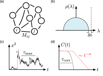
Figure 1: Schematics. A linear dynamical system with damping and pairwise interaction $M$ has time scales determined by the eigenvalue spectrum of $M$, especially the gap $g_{0}$ to the stability threshold. If the system is perturbed (red arrow), the norm activity decays with a longest time scale $\tau_{\text{max}}=1/g_{0}$, while the correlations in the unperturbed system decay with a characteristic time scale, defined to be the correlation time $\tau_{\text{corr}}$. In cases where the system has a continuous range of long time scales, the correlations decay as a power law (red curve). Systems with long time scales are defined such that $\tau_{\text{max}}$ and $\tau_{\text{corr}}$ grow as system size $N$.

When we say that we want to search for long time scales, there are two possibilities. One is that we are interested in the single longest time scale, and the other is that we are interested in the full range of time scales. To get at these different questions, we define the longest time scale of the system, $\tau_{\text{max}}$, and the correlation time scale, $\tau_{\text{corr}}$. We continue to think about the case where $M$ is symmetric, and return to the more general case in the discussion.

Longest time scale. The longest time scale, $\tau_{\text{max}}$, is the time constant given by the slowest mode of the system, which dominates the dynamics after long enough times. This time scale is determined by the gap, $g_{0}$, between the largest eigenvalue and the stability threshold, which with our choice of units is $w=1$. Mathematically, we define

$$\tau_{\text{max}}\equiv\frac{1}{g_{0}}=\frac{1}{1-\lambda_{\text{max}}}.$$ (6)

In the thermodynamic limit, the gap is taken to be between the stability threshold and the right edge of the support of the spectral density.

Correlation time. To get at the correlation time, let’s take seriously the idea that the network is driven by noise. Then $x(t)$ become a stochastic process, and from Eqs (1) and (2) we can calculate the correlation function

$$\begin{split}C_{N}(t)&\equiv\frac{1}{N}\sum_{i}\langle x_{i}(0)x_{i}(t)\rangle\\ &=\frac{1}{N}\sum_{i}\frac{1}{1-\lambda_{i}}e^{-(1-\lambda_{i})|t|}\\ &=\frac{1}{N}\sum\tau_{i}e^{-|t|/\tau_{i}}.\end{split}$$ (7)

The normalized correlation function

$$R_{N}(t)\equiv\frac{C_{N}(t)}{C_{N}(0)}=\frac{\sum_{i}\tau_{i}e^{-|t|/\tau_{i}}}{\sum_{i}\tau_{i}}$$ (8)

has the intuitive behavior of starting at $R_{N}(0)=1$ and decaying monotonically. Then there is a natural definition of the correlation time, by analogy with single exponential decays,

$$\tau_{\text{corr}}(\{\lambda\})\equiv\int_{0}^{\infty}dt\,R_{N}(t)=\frac{\sum_{i}\tau_{i}^{2}}{\sum_{i}\tau_{i}}.$$ (9)

In the thermodynamic limit, the autocorrelation coefficient $R(t)$ and the correlation time $\tau_{\text{corr}}$ becomes the ratio of two integrals over the eigenvalue density $\rho(\lambda)$.

Importantly, $\tau_{\text{max}}$ depends only on the largest eigenvalue, while $\tau_{\text{corr}}$ depends on the entire spectrum, and hence can be used to differentiate cases where the system is dominated by a single vs. a continuous spectrum of slow modes. The two time scales satisfy $\tau_{\text{corr}}\leq\tau_{\text{max}}$, with the equality assumed only when all eigenvalues are equal, i.e. the spectral density is a delta function at $\lambda=\lambda_{\text{max}}$.

With these definitions, we refine our goal as to find biologically plausible ensembles for the connection matrix $M$, such that the resulting stochastic linear dynamics has time scales, $\tau_{\text{max}}$ and $\tau_{\text{corr}}$, that are “long,” growing as a power of the system size $N$, perhaps even extensively. To avoid fine tuning, we will construct examples of such ensembles by imposing global constraints on measurable observables of the dynamical system. We then compute the spectral density and the corresponding time scales using a combination of mean-field theory and numerical sampling of finite systems.

III Time scales for ensembles with different global constraints

To construct linear dynamical systems that generate long time scales without fine tuning individual parameters, we want to find probability distributions $P(M)$ for the connection matrix such that time scales are long, on average. We start with the simplest Gaussian distribution, the GOE above, and gradually add constraints. We will see that for the GOE itself, there is a critical value of the scaled variance $c_{\text{crit}}^{2}=1/2$. For $c<c_{\text{crit}}$ the system is stable but time scales are short, while for $c>c_{\text{crit}}$ the system is unstable. Exactly at the critical point $c=c_{\text{crit}}$ time scales are long in the sense that we have defined, diverging with system size. The essential challenge is to find the weakest constraints on $P(M)$ that make these long time scales generic. Many of the results that weneed along the way are known in the random matrix theory literature, but we will arrive at some new theoretical questions.

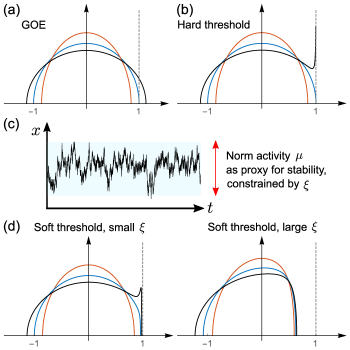
Figure 2: Spectral density for the connection matrix $M$ drawn from the Gaussian Orthogonal Ensemble (GOE, a), the GOE with a hard threshold enforcing stability (hard threshold, b), and the GOE with an additional global constraint on the norm activity (soft threshold, d). Three representative parameters are chosen for each ensemble such that the system is subcritical ($c=0.6$, red), critical ($c=1/\sqrt{2}$, blue), and supercritical ($c=0.8$, black). The stability threshold is visualized as the dashed gray line at $\lambda_{w}=1$. Panel (c) is a schematic for constraining the averaged norm activity, generating ensembles with the soft threshold.

III.1 Model 1: the Gaussian Orthogonal Ensemble

The simplest ensemble for the interaction matrix $M$ is the Gaussian Orthogonal Ensemble (GOE) without any additional constraints, which has been studied since the beginning of random matrix theory wigner_on_1951 ; dyson_threefold_1962 ; dyson_brownianmotion_1962 ; livan_introduction_2018 . Mathematically, we have $M=M^{\intercal}$, and

$$P(M)\propto\exp\left(-\frac{N}{2c^{2}}\text{Tr}M^{\intercal}M\right);$$ (10)

since $c$ sets the scale of synaptic connections, we will refer to this parameter as the interaction strength. Because the distribution only depends on matrix traces, it is invariant to rotations of $M$. Equivalently, if we think of decomposing the matrix $M$ into its eigenvectors and eigenvalues, the probability depends only on the eigenvalues. Thus, we can integrate out the eigenvectors, and obtain the joint distribution of eigenvalues,

$$P_{\text{GOE}}(\{\lambda_{i}\})\propto\exp\left[-\frac{N}{2c^{2}}\sum_{i}\lambda_{i}^{2}+\frac{1}{2}\sum_{j\neq k}\ln\big{\lvert}\lambda_{j}-\lambda_{k}\big{\rvert}\right],$$ (11)

where the logarithmic repulsion term emerges from the Jacobian when we change variables from matrix elements to eigenvalues and eigenvectors. The spectral density can then be found using a mean field approximation, which becomes exact as $N\rightarrow\infty$. The result is Wigner’s well-known semicircle distribution wigner_on_1951 ,

$$\rho_{\text{GOE}}(\lambda)=\frac{1}{\pi c}\sqrt{2-\frac{\lambda^{2}}{c^{2}}},\hskip 28.45274pt\lambda\in[-\sqrt{2}c,\sqrt{2}c].$$ (12)

For completeness, we review the derivation of the spectral density in Appendix A.

Equation (12) for the spectral density, together with Fig 2a, shows that there is a phase transition at $c_{\text{crit}}=1/\sqrt{2}$. If the interaction strength is greater than this critical strength (supercritical), then $\lambda_{\text{max}}>1$ and the system becomes unstable. If the interaction strength is smaller (subcritical), then the gap size between the largest eigenvalue and the stability threshold $\lambda=1$ is of order 1, and the time scales remain finite as system size increases. The only case when the system has slow modes is at the critical value of the interaction strength, $c=c_{\text{crit}}=1/\sqrt{2}$, where the spectral density becomes tangential to the stability threshold.

At criticality, corresponding to the blue curve in Fig 2a, we can estimate the size of the gap by asking that the gap be large enough to contain $\sim 1$ mode, that is

$$\int_{1-g_{0}}^{1}d\lambda\,N\rho(\lambda)\sim 1.$$ (13)

With $\rho(\lambda)\sim(1-\lambda)^{1/2}$, this gives $Ng_{0}^{3/2}\sim 1$ or $g_{0}\sim N^{-2/3}$. Thus the longest time scale grows with system size, $\tau_{\text{max}}\sim N^{2/3}$.

In the same way, we can estimate the full correlation function from the correlation time [Eq (7)],

$$C_{N}(t) = \frac{1}{N}\sum\tau_{i}e^{-t/\tau_{i}}$$ (14)

$$= \int d\lambda{{\rho(\lambda)}\over{(1-\lambda)}}e^{-(1-\lambda)|t|}$$

$$\sim \int d\lambda{{1}\over{(1-\lambda)^{1/2}}}e^{-(1-\lambda)|t|}\sim|t|^{-1/2}.$$ (15)

This has the power–law behavior expected for a critical system, where there is a continuum of slow modes.

Note that in the GOE system, slow modes with time scales growing as system size are only possible at a single value of the interaction strength. Nonetheless, we need to distinguish the fine tuning here as happening at an ensemble level, which is different from the element-wise fine tuning that might have been required if we considered particular interaction matrices.

III.2 Model 2: GOE with hard stability threshold

Drawing interaction matrices from the GOE leads to long time scales only at a critical value of interaction strength. Can we modify the ensemble such that long time scales can be achieved without this fine tuning? In particular, in the GOE, if the interaction strength is too large, then the system becomes unstable. What will the spectral distribution look like if we allow $c>c_{\text{crit}}$ but edit out of the ensemble any matrix that leads to instability?

Mathematically, a global constraint on the system stability requires all eigenvalues to be less than the stability threshold, $\lambda_{w}=1$. This modifies the eigenvalue distribution with a Heaviside step function:

$$P_{\text{hard}}(\{\lambda_{i}\})\propto P_{\text{GOE}}(\{\lambda_{i}\})\prod_{i}\Theta(1-\lambda_{i}).$$ (16)

Conceptually, what this model does is to pull matrices out of the GOE and discard them if they produce unstable dynamics; the distribution $P_{\text{hard}}(\{\lambda\})$ describes the matrices that remain after this editing. Importantly we do not introduce any extra structure, and in this sense $P_{\text{hard}}$ is a maximum entropy distribution, as discussed more fully below.

The spectral density $\rho(\lambda)$ that follows from $P_{\text{hard}}$ was first found by Dean and Majumdar dean_large_2006 ; dean_extreme_2008 ; majumdar_top_2014 . Again, there is a phase transition depending on the interaction strength. For ensembles with interaction strength less than the critical value $c_{\text{crit}}=1/\sqrt{2}$, the stability threshold is away from the bulk spectrum, so the spectral density remains as Wigner’s semicircle. On the other hand, if the interaction strength is greater than the critical value, the spectral density becomes

$$\rho(\lambda)=\frac{1}{c^{2}}\frac{\sqrt{\lambda+l^{*}-1}}{2\pi\sqrt{1-\lambda}}\left(l^{*}-2\lambda\right),$$ (17)

where

$$l^{*}=\frac{2}{3}\left(1+\sqrt{1+6c^{2}}\right).$$

As shown in Fig 2b, the stability threshold acts as a wall pushing the eigenvalues to pile up. More precisely, near the stability thresshold $\lambda=1$ we have $\rho(\lambda)\sim(1-\lambda)^{-1/2}$, which [by the same argument as in Eq (13)] indicates that the longest time scale increases as system size with $\tau_{\text{max}}\sim N^{2}$.

The autocorrelation function also is dominated by the eigenvalues close to the stability threshold. The calculation is a bit subtle, however, since

$$C(t)=\int d\lambda{{\rho(\lambda)}\over{(1-\lambda)}}e^{-(1-\lambda)|t|}\sim\int dk\,k^{-1/2}\,k^{-1}\,e^{-k|t|}$$

is not integrable. After introducing an IR cut-off at $\varepsilon\sim g_{0}\sim N^{-2}$, we can write the resulting autocorrelation coefficient as

$$R(t)=\frac{C(t)}{C(0)}=1-\sqrt{\pi}(\varepsilon t)^{1/2}+\varepsilon t+\mathcal{O}((\varepsilon t)^{2}).$$ (18)

The correlation time

$$\tau_{\text{corr}}=\frac{\int_{\varepsilon}dk\rho(k)k^{-2}}{\int_{\varepsilon}dk\rho(k)k^{-1}}\sim\frac{\int_{\varepsilon}dkk^{-5/2}}{\int_{\varepsilon}dkk^{-3/2}}\sim\varepsilon^{-1}\sim N^{2}.$$ (19)

We see that for supercritical systems, both the longest time scale $\tau_{\text{max}}$ and the correlation time $\tau_{\text{corr}}$ increase as a power of the system size; the rate is even faster than the system at criticality. In fact, there are divergently many slow modes. Meanwhile, the interaction strength can undertake a range of values, as long as they are greater than a certain threshold. Thus it would seem that we have overcome the fine tuning problem!

In fact, we cannot quite claim that the problem is solved. First, in the supercritical phase, the correlation function does not decay as a power law. Instead, the correlation function stays at 1 for a time period $\tau_{\text{corr}}\sim\tau_{\rm max}$, and then decays exponentially. This means the system has a single long time scale, rather than a continuous spectrum of slow modes. Second, in order for a system to impose a hard constraint on its stability, it needs to measure its stability. Naively, checking for stability, especially in the presence of slow modes, requires access to infinitely long measuring times; implementing a sharp threshold may also be challenging.

III.3 Model 3: Constraining mean-square activity

While it can be difficult to check for stability, it is much easier to imagine checking the overall level of activity in the network. One can even think about mechanisms that would couple indirectly to activity, such as the metabolic load. If the total activity is larger than some target level, the system might be veering toward instability, and there could be feedback mechanisms to reduce the overall strength of connections. Regulation of this qualitative form is known to occur in the brain, and is termed synaptic scaling turrigiano_activity-dependent_1998 ; turrigiano_homeostatic_2004 ; abbott_synaptic_2000 ; this is hypothesized to play an important role in maintaining persistent neural activities renart_robust_2003 ; tetzlaff_synaptic_2013 . In this section, we construct the least structured distribution $P(M)$ that is consistent with a fixed mean (square) level of activity, which we can think of as a soft threshold on stability, and derive the density of eigenvalues that follow from this distribution. In the following section we discuss possible mechanisms for a system to generate matrices $M$, dynamically, out of this ensemble.

III.3.1 The spectral density

It is useful to remember that the GOE, Eq (10), can be seen as the maximum entropy distribution of matrices consistent with some fixed variance of the matrix elements $M_{ij}$  jaynes57 ; presse_principles_2013 . If we want to add a constraint, we can stay within the maximum entropy framework, and in this way we isolate the generic consequences of this constraint: we are constructing the least structured ensemble of networks that satisfies the added condition.

We recall that if we want to constrain the mean values of several functions $f_{\mu}(M)$, then the maximum entropy distribution has the form

$$P(M)={1\over Z}\exp\left[-\sum_{\mu}g_{\mu}f_{\mu}(M)\right].$$ (20)

In our case are are interested in the mean–square value of the individual matrix elements, and the mean–square value of the activity variables $x_{i}$. But our basic model Eqs (1) and (2) predicts that

$$\mu={1\over N}\sum_{i}\langle x^{2}_{i}\rangle={1\over N}\sum_{i}{1\over{1-\lambda_{i}}},$$ (21)

so the relevant maximum entropy model becomes

$$P(M)={1\over Z}\exp\left[-\frac{N}{2c^{2}}\text{Tr}M^{\intercal}M-N\xi\sum_{i}\frac{1}{1-\lambda_{i}}\right].$$ (22)

Again, this distribution is invariant to orthogonal transformation. After the integration over the rotation matrices, we have

$$P(\{\lambda_{i}\})\propto\exp\left[-\frac{N}{2c^{2}}\sum_{i}\lambda_{i}^{2}+\frac{1}{2}\sum_{j\neq k}\ln\big{\lvert}\lambda_{j}-\lambda_{k}\big{\rvert}-N\xi\sum_{i}\frac{1}{1-\lambda_{i}}\right],$$ (23)

where the scaling $N\xi$ ensures that all the terms in the exponent are $\sim N^{2}$, so there will be a well defined thermodynamic limit. Luckily, the same arguments that yield the exact density of eigenvalues in the Gaussian Orthogonal Ensemble also work here (see Appendix A), and we find

$$\rho(\lambda)=\frac{1}{\pi\sqrt{(\lambda-1+g_{0}+l)(1-g_{0}-\lambda)}}\left[1+\frac{l^{2}}{8c^{2}}+\left(1-g_{0}-\frac{1}{2}l\right)\frac{\lambda}{c^{2}}-\frac{\lambda^{2}}{c^{2}}+\frac{\xi}{2}\frac{(2g_{0}-2g_{0}^{2}+l-2g_{0}l)-(2g_{0}+l)\lambda}{\sqrt{g_{0}(g_{0}+l)}(\lambda-1)^{2}}\right]\mbox{,}$$ (24)

where the gap size $g_{0}$ and the width of the support $l$ are fixed by setting the spectral density at the two ends of the support zero.

To our surprise, we find a finite gap for all $\xi>0$. This means that there exists a maximum time scale even when the system is infinitely large. This upper limit of longest time scale depends on the Lagrange multiplier $\xi$ and the interaction strength $c$. Because the Lagrange multiplier $\xi$ is used to constrain the averaged norm activity $\mu$, the maximum time scale is set by the allowed norm of the activity $\mu$, measured in units of expected norm for independent neurons. As we explain below, the greater dynamic range the system can allow leads to longer time scales.

The dependence of the gap on the Lagrange multiplier $\xi$ is shown in Fig 2d at each of several fixed values of $c$; as before there is a phase transition at $c_{\text{crit}}=1/\sqrt{2}$. This is understandable, since in the limit of $\xi=0$ we recover the hard wall case. For small $\xi$, the spectrum is similar to the hard wall case, with the eigenvalues close to the stability threshold pushed into the bulk spectrum; for large $\xi$, the entire spectrum is pushed away from the wall. A closer look at the longest time scale $\tau_{\text{max}}$ vs. Lagrange multiplier in Fig. 3a confirms that amplification of time scales occurs only when $\xi<1$, corresponding to an amplification of mean–square activity $\mu$.

III.3.2 The scaling of time scales in three phases

We now discuss the dependence of time scales on the interaction strength $c$. In contrast to the ensemble with a hard stability threshold, we find a finite gap for all values of interaction strength $c$, but the scaling of time scales vs. the Lagrange multiplier (and hence the mean–square activity) is different in the different phases.

For the subcritical and critical phases, the results are as expected from the hard wall case. In the subcritical phase, as $\xi\rightarrow 0$, the spectral distribution converges smoothly to the familiar semicircle. The time scales and the mean–square activity both approach constants. On the other hand, when $c=c_{\text{crit}}$, we find that the longest time scale grows as $\tau_{\text{max}}\sim\xi^{-2/5}$, and the correlation time scale $\tau_{\text{corr}}\sim\xi^{-1/5}$, i.e. both time scales can be large if $\xi$ is small enough; meanwhile, the norm activity $\mu$ approaches a constant value of $\mu=2$. This suggests that if a system is poised at criticality, then the system can exhibit long time scales, even when the dynamic range of individual components is well controlled. The autocorrelation function exhibits a power law-like decay, as expected; see the blue curve in Fig 3f.

The most interesting case is the supercritical phase, where the interaction strength $c>c_{\text{crit}}=1/\sqrt{2}$. As $\xi\rightarrow 0$, the spectrum does not converge to the spectrum with the hard constraint. We find that both time scales and the norm activity increase as power laws of the Lagrange multiplier $\xi$ (Fig 3), with $\tau_{\text{max}}\approx 3\tau_{\text{corr}}\sim\xi^{-2/3}$, and $\mu\sim\xi^{-1/3}$. This implies that the time scales grow as a power of the allowed dynamic range of the system, although not with the size of the system. The question of whether the resulting time scales are “long” then becomes more subtle. Quantitatively, we see from Fig 3c, that if the system has an allowed dynamic range just $10\times$ that of independent neurons, the system can generate time scales $\tau_{\text{max}}$ almost $10^{4}\times$ longer than the time scale of isolated neurons.

Interestingly, once the system is in the supercritical phase, the ratio of amplification has only a small dependence on the interaction strength $c$ (Fig 3e). Intuitively, while an increasing interaction strength $c$ implies that without constraints more modes will be unstable, while with constraints more modes concentrate near the stability threshold, but the entire support of the spectrum also expands, so the density of slow modes and their distance to the stability threshold remain similar. This is perhaps another indication for long time scales without fine tuning when the system uses its norm activity to regulate its connection matrix.

We note that, although both the critical phase and the supercritical phase can reach time scales that are as long as the dynamic range allows, there are significant differences between the two phases. One difference is that in the critical phase, locally the dynamic range for each neuron can remain finite, while for the supercritical phase, the variance of activity for individual neurons can be much greater. Moreover, as shown by Fig. 3f, systems in the supercritical phase are dominated by a single slow mode, rather than by a continuous spectrum of slow modes. While the autocorrelation function decays as a power law in the critical phase, in the supercritical phase, it holds at $R(t)=1$ for a much longer time compared to the subcritical case, but then decays exponentially. While a single long time scale can be achieved without fine tuning, it seems that a continuous spectrum of long time scales is much more challenging.

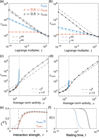
Figure 3: Mean field results for Model 3. The longest time scale $\tau_{\text{max}}$ (a) and the correlation time scale $\tau_{\text{corr}}$ (b) increase with different scaling as the Lagrange multiplier $\xi$ decreases, corresponding to an increasing value for the constrained averaged norm activity, $\mu$ (c,d). The exact scaling and the amplification of time constant depending on whether the system is subcritical (with interaction strength $c<1/\sqrt{2}$), critical ($c=1/\sqrt{2}$), or supercritical (e). Despite the supercritical phase exhibit long time scales, the autocorrelation function decays as a power law only at $c=c_{\text{crit}}$, and as exponential for other values of interaction strength (f). For this panel, $\xi=10^{-10}$, red curves are for $c=0.2$, $c=0.6$, blue curve is at $c=c_{\text{crit}}$, and black curves are at $c=1$ and $c=3$.

III.3.3 Finite Size Effects

If we want these ideas to be relevant to real biological systems, we need to understand what happens at finite $N$. We investigate this numerically using direct Monte-Carlo sampling of the (joint) eigenvalue distribution. As the system size grows the time scales $\tau_{\text{max}}$ and $\tau_{\text{corr}}$ also grow, up to the upper limit given by the mean field results; see Fig 4. Finite size scaling is difficult in this case, since the scaling exponent $\alpha$ for the gap difference,

$$\Delta g_{0}(N)\equiv g_{0}(N)-g_{0}\sim N^{\alpha},$$ (25)

depends on the Lagrange multiplier $\xi$ (Fig 4e,f). In particular, the scaling interpolates between two limiting cases: for small $\xi$, the gap scales as $\Delta g_{0}\sim N^{-2}$, as in the universality class of the hard threshold; for large $\xi$, the gap scales as $\Delta g_{0}\sim N^{-2/3}$, which is in the universality class of the Gaussian ensemble without any additional constraint. In any case, thousands of neurons will be well described by the $N\rightarrow\infty$ limit.

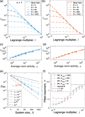
Figure 4: Finite size effects on the time scales $\tau_{\text{max}}$ and $\tau_{\text{corr}}$ for Model 3, interaction strength $c=1$ (the supercritical phase). Results from direct Monte Carlo sampling of the eigenvalue distribution are plotted together with the mean field results. There is no universal exponent that explains the convergence of $\tau_{\text{max}}$ when system size increases (e), and apparent exponents $\alpha$ depend on the Lagrange multiplier $\xi$. Panel f shows that the apparent $\alpha$ depends on the maximum system size used in the fitting, interpolating between $\alpha=2$ and $\alpha=2/3$.

III.3.4 Distribution of matrix elements

Now that we have examples of network ensembles that exhibit long time scales, we need to go back and check what these ensembles predict for the distribution of individual matrix elements. In particular, because we did not constrain the self interaction $M_{ii}$ to be 0, we want to check whether the long time scales emerge as a collective behavior of the network, or trivially from an effective increase of the intrinsic time scales for individual neurons, $\tau_{\text{ind}}^{\text{eff}}=1/(1-\langle M_{ii}\rangle)=1/(1-\langle\lambda\rangle)$. A similar question arises in real networks, where there have been debates about the importance of feedback within single neurons vs. the network dynamics in maintaining long time scales; see Ref  major_persistent_2004 for a review. We confirm that, at least in our models, this is not an issue: the constraint on the norm activity, in fact, pushes the average eigenvalues to be negative, and hence the effective self interaction for individual neurons actually leads to a shorter intrinsic time scale. We can impose additional constraints on the distribution of matrix elements, such that $\langle M_{ii}\rangle=0$; for this ensemble, we can again solve for the spectral distribution, and we find that scaling behaviors described above don’t change.

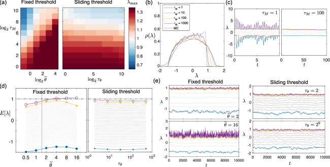
Figure 5: A neural network can tune its connection matrix to the ensemble with slow modes using simple Langevin dynamics. Two candidates for the dynamics include one with a fixed threshold on the averaged neural activity, and one with a sliding threshold. (a) Average $\lambda_{\text{max}}$. With fixed threshold (left), the system is stable only if the updating time scale $\tau_{M}$ is long enough, and if the fixed threshold for the norm activity, $\widetilde{\theta}$, is small enough, thus requiring fine tuning. With a sliding threshold (right), the system is stable for a large range of $\tau_{\theta}$. (b) The spectral distribution for connection matrix drawn from the dynamics with fixed threshold approaches the static distribution as the time constant $\tau_{M}$ increases. (c) If the connection matrix updates too fast, i.e. $\tau_{M}$ is too small, the system exhibits quasi-periodic oscillations, and does not reach a steady state distribution. In contrast, long $\tau_{M}$ leads to the adiabatic approximation for the steady state distribution. (d) The expected eigenvalues for the dynamics with fixed threshold, and for the ones with sliding threshold, wiith $N=32$, $c=1$, $\xi=2^{-5}$ and $\tau_{M}=1000$. (e) Example traces for the eigenvalues vs. time.

III.4 Dynamic tuning

So far, we have established that a distribution constraining the norm activity can lead generically to long time scales, but we haven’t really found a mechanism for implementing this idea. But if we can write the distribution of connection matrices $M$ in the form a Boltzmann distribution, we know that we can sample this distribution by allowing the matrix elements be dynamical variables undergoing Brownian motion in the effective potential. We will see that this sort of dynamics is closely related to previous work on self–tuning to criticality  magnasco_self-tuned_2009 , and we can interpret the dynamics as implementing familiar ideas about synaptic dynamics, such as Hebbian learning and metaplasticity.

We can rewrite our model in Eq (22) as

$$P(M) = {1\over Z}\exp\left[-\frac{N}{2c^{2}}\text{Tr}M^{\intercal}M-N\xi\sum_{i}\frac{1}{1-\lambda_{i}}\right]$$ (26)

$$= {1\over Z}\exp\left[-V(M)/T\right]$$

$$V(M) = \frac{1}{2}\text{Tr}M^{\intercal}M+c^{2}\xi\text{Tr}(1-M)^{-1},$$ (27)

with a temperature $T=c^{2}/N$. The matrix $M$ will be drawn from the distribution $P(M)$, as $M$ itself performs Brownian motion or Langevin dynamics in the potential $V(M)$:

$$\begin{split}\tau_{M}\dot{M}&=-\frac{\partial V(M)}{\partial M}+\zeta(t)\\ &=-M-c^{2}\xi(\mathbf{1}-M)^{-2}+\zeta(t),\end{split}$$ (28)

where the noise has zero mean, $\langle\zeta\rangle=0$, and is independent for each matrix element,

$$\langle\zeta_{ij}(t)\zeta_{kl}(t^{\prime})\rangle=2T\tau_{M}\delta_{ik}\delta_{jl}\delta(t-t^{\prime}).$$ (29)

It is useful to remember that, in steady state, our dynamical model for the $\{x_{i}\}$, Eqs (1) and (2), predicts that

$$\langle x_{i}x_{j}\rangle=[(\mathbf{1}-M)^{-1}]_{ij}.$$ (30)

This means that we can rewrite the Langevin dynamics of $M$, element by element, as

$$\tau_{M}\dot{M}_{ij} = -M_{ij}-c^{2}\xi[(\mathbf{1}-M)^{-2}]_{ij}+\zeta_{ij}(t)$$ (31)

$$= -M_{ij}-c^{2}\xi\langle x_{i}x_{k}\rangle\langle x_{k}x_{j}\rangle+\zeta_{ij}(t).$$

Because the $x_{i}$ are Gaussian, we have

$$\langle x_{i}x_{k}\rangle\langle x_{k}x_{j}\rangle={1\over 2}\left(\langle x_{i}x_{k}x_{k}x_{j}\rangle-\langle x_{i}x_{j}\rangle\langle x_{k}x_{k}\rangle\right),$$ (32)

where as above the summation over the repeated index $k$ is understood, so that

$$\langle x_{i}x_{k}\rangle\langle x_{k}x_{j}\rangle={1\over 2}{\bigg{\langle}}x_{i}x_{j}\left(\sum_{k}x_{k}^{2}-\sum_{k}\langle x_{k}^{2}\rangle\right){\bigg{\rangle}}.$$ (33)

We now imagine that the dynamics of $M$ is sufficiently slow that we can replace averages by instantaneous values, and let the dynamics of $M$ do the averaging for us. In this approximation we have

$$\tau_{M}\dot{M}_{ij}=-M_{ij}-{1\over 2}c^{2}\xi x_{i}x_{j}\left(\sum_{k}x_{k}^{2}-\theta\right)+\zeta_{ij}(t),$$ (34)

where the threshold $\theta=\sum_{k}\langle x_{k}^{2}\rangle$.

The terms in this Langevin dynamics have a natural biological interpretation. First, the connection strength decays with an overall time constant $\tau_{M}$. Second, the synaptic connection $M_{ij}$ is driven by the correlation between pre– and post–synaptic activity, $\sim x_{i}x_{j}$, as in Hebbian learning hebb_organization_1949 ; magee_synaptic_2020 . In more detail, we see that the response to correlations is modulated depending on whether the global neural activity is greater or less than a threshold value; if the network is highly active, then the connection between neurons with correlated activity will decrease, i.e. the dynamics are anti-Hebbian, while and if the overall network is quiet the dynamics are Hebbian.

We still have the problem of setting the threshold $\theta$. Ideally, for the dynamics to generate samples out of the correct $P(M)$, we need

$$\theta=\theta^{*}\equiv\langle x^{\intercal}x\rangle_{\text{s.s.}}=N\mu(c,\xi),$$ (35)

where as above $\mu$ is the mean activity whose value is enforced by the Lagrange multiplier $\xi$. This means that $\theta$ needs to be tuned in relation to $\xi$, and it is challenging to have a mechanism that does this directly, and just pushes the fine tuning problem back one step. Importantly, if $\theta=\theta^{*}$ then the steady state spectral density of the connection matrix approaches the desired equilibrium distribution as the update time constant increases (Fig 5b), but if $\theta$ deviates from $\theta^{*}$ then the steady distribution does not have slow modes. As shown in Fig 5de, if the threshold is too small, then the entire spectrum is shifted away from the stability threshold, and the system no longer exhibits long time scales; if the threshold is too large, then the largest eigenvalue oscillates around the stability threshold $\lambda=1$, and a typical connection matrix drawn from the steady state distribution is unstable.

But we can once again relieve the fine tuning problem by promoting $\theta$ to a dynamical variable,

$$\tau_{\theta}\dot{\theta}=\sum_{k}x_{k}^{2}-\theta,$$ (36)

which we can think of as a sliding threshold in the spirit of models for metaplasticity bcm_1982 . We pay the price of introducing yet another new time scale, $\tau_{\theta}$, but in Figs 5de we see that this can vary over at least three orders of magnitude without significantly changing the spectral density of the eigenvalues.

To see whether the sliding threshold really works, we can compare results where $\theta$ is fixed to those where it changes dynamically; we follow the mean value of $\lambda_{\text{max}}$ as an indicator of system performance. We choose parameters in the supercritical phase, specifically $c=1$ and $\xi=2^{-5}$, and study a system with $N=32$. Figure 5a shows that with fixed threshold, even in the adiabatic limit where $\tau_{M}\gg 1$, there is only a measure-zero range for the fixed threshold $\widetilde{\theta}$ such that $\lambda_{\text{max}}$ is very close to, but smaller than $1$. In contrast, for the dynamics with sliding threshold, at $\tau_{M}\gg 1$ there is a large range of values for the time constant $\tau_{\theta}$ such that the system hovers just below instability, generating a long time scale.

The Langevin dynamics of our system is similar to the BCM theory of metaplasticity in neural networks, in that both models involve a combination of Hebbian learning and a threshold on the neural activity bcm_1982 , but there are two key differences. First, the BCM theory imposes a threshold on the activity of locally connected neurons, while here the threshold is on the overall neural activity. Second, the BCM dynamics is Hebbian when the post– and pre–synaptic activities are larger than the threshold, and anti–Hebbian otherwise, which is the opposite of the dynamics for our system. It is interesting that in some other models for homeostasis, plasticity requires the activity detection mechanism to be fast ($\tau_{\theta}/\tau_{M}\ll 1$) for the system to be stable zenke_synaptic_2013 ; zenke_temporal_2017 , which we do not observe for our system.

IV Discussion

Living systems can generate behaviors on time scales that are much longer than the typical time scales of their component parts, and in some cases correlations in these behaviors decay as an approximate power–law, suggesting a continuous spetcrum of slow modes. In order to understand how surprised we should be by these behaviors, it is essential to ask whether there exist biologically plausible dynamical systems that can generate these long time scales “easily.” Typically, to achieve long time scales a high dimensional dynamical system requires some degree of fine tuning: from the most to the least stringent, examples include setting individual elements of the connection matrix, choosing a particular network architecture, or imposing some global constraints which allow ensembles of systems with long time scales.

In this note, we were able to construct a mechanism for living systems to reach long time scales with the least stringent fine-tuning condition: when the interaction strength of the connection matrix is large enough, imposing a global constraint on the stability of the system leads to divergent many slow modes. To impose a biologically plausible mechanism for living systems, we constrain the averaged norm activity as a proxy for global stability; in this case, the time scales for the slow modes are set by the allowed dynamic range of the system. Further, we showed that these ensembles can be achieved by updating the connection matrix $M$ with a sliding threshold for the norm activity, a mechanism that resembles metaplasticity in neural networks.

Importantly, the slow modes achieved through constraining norm activity typically lead to exponentially decaying correlations; only when the interaction strength of the matrix is at a critical value do we find power-law decays. This suggest that a continuous range of slow modes is more difficult to achieve than a single long time scale. A natural follow-up question is whether there exist mechanisms which can tune the system to criticality in a self-organized way, for example by coupling the interaction strength to the averaged norm activity.

Both for simplicity and to understand the most basic picture, we have been focusing on linear networks with symmetric connections. Realistically, many biological networks are asymmetric, which gives rise to more complex and perhaps even chaotic dynamics sompolinsky_chaos_1988 ; vreeswijk_chaos_1996 . In the asymmetric case, the eigenvalue spectrum for the Gaussian ensemble is well known (uniform distribution inside a unit circle) ginibre_statistical_1965 ; forrester_eigenvalue_2007 , but a similar global constraint on the norm activity leads to a dependence on the overlap among the left and right eigenvectors chalker_eigenvector_1998 ; mehlig_statistical_2000 . In particular, the matrix distribution can no longer be separated into the product of eigenvalues and eigenvectors, and it is difficult to solve for the spectral distribution analytically. Two new features emerge in the asymmetric case. First, the time scales given by real eigenvalues vs. complex eigenvalues may be different, leading to more (or less) dominant oscillatory slow modes in large systems akemann_integrable_2007 . Second, asymmetric connection matrices can lead to complicated transient activity when the system is perturbed, with the time scales mostly dominated by the eigenvector overlaps, and can be very different from the time scales given by the eigenvalues grela_what_2017 . In the limit of strong asymmetry, the network is organized into a feed-forward line, information can be held for a time that is extensive in system size; see examples in Refs. goldman_memory_2009 and ganguli_memory_2008 . It will be interesting to check whether systems can store information in these transients without fine-tuning the structure of the network.

The system we study can be extended to consider more specific ensembles for particular biological systems. For example, real neural networks have inhibitory and excitatory neurons, so that elements belonging to the same column need to share the same sign, and the resulting spectral distribution has been shown to differ from the unit sphere rajan_eigenvalue_2006 ; more generally recent work explores how structured connectivity can lead to new but still universal dynamics tarnowski_universal_2019 . Another limitation of our work is that it only considers linear dynamics, or only dynamical systems where all fixed points to be equally likely. In contrast, some non-linear dynamics such as the Lotka-Volterra model in ecology biroli_marginally_2018 , and the gating neural network in machine learning can_gating_2020 ; krishnamurthy_theory_2020 have been shown to drive systems to non-generic, marginally stable fixed points, around which there exists an extensive number of slow directions for the dynamics. In summary, we believe the issue of whether a continuum of slow modes can arise generically in neural networks remains open, but we hope that our study of very simple models has helped to clarify this question.

Appendix A Spectral distribution for the Gaussian Orthogonal Ensemble

For completeness, we sketch here the well-known derivation of the spectral density for random matrices drawn from the Gaussian Orthogonal Ensemble wigner_on_1951 ; dyson_threefold_1962 ; dyson_brownianmotion_1962 . Excellent pedagogical discussions can be found in Refs marino_number_2016 ; livan_introduction_2018 . These same methods allow us to derive the spectral densities in all the other cases that we consider in the main text.

Let $M$ be a matrix with size $N\times N$. Assume $M$ is real symmetric, and that the individual elements of the $M$ matrix are independent gaussian random numbers,

$$M_{ii}\sim\mathcal{N}(0,1/N),$$ (37)

$$M_{ij}|_{i\neq j}\sim\mathcal{N}(0,1/2N).$$ (38)

This is the Gaussian Orthogonal Ensemble (GOE). Together with its complex and quaternion counterparts, the Gaussian Ensembles are the only random matrix ensembles that both have independent entries and are invariant under orthogonal (unitary, symplectic) transformations, which is more obvious when we write the probability distribution of $M$ in terms of its trace:

$$P(M)\propto\exp\left(-\frac{N}{2}\text{Tr}M^{\intercal}M\right).$$ (39)

Symmetric matrices can be diagonalized by orthogonal transformations,

$$M=O^{\intercal}\Lambda O,$$ (40)

where the matrix $O$ is constructed out of the eigenvectors of $M$ and the matrix $\Lambda$ is diagonal with elements given by the eigenvalues $\{\lambda_{i}\}$. Because $P(M)$ is invariant to orthogonal transformations of $M$, it is natural to integrate over these transformations and obtain the joint distribution of eigenvalues. To do this we need the Jacobian, also called the Vandermonde determinant,

$$dM=\prod_{i<j}\lvert\lambda_{i}-\lambda_{j}|d\mu(O)\prod_{i=1}^{N}d\lambda_{i},$$ (41)

where $d\mu(O)$ is the Haar measure of the orthogonal group under its own action. Now we can integrate over the matrices $O$, or equivalently over the eigenvectors, to obtain

$$P(\{\lambda_{i}\})\prod_{i=1}^{N}d\lambda_{i} = \int d\mu(O)\prod_{i<j}\lvert\lambda_{i}-\lambda_{j}|\,P(M)\prod_{i=1}^{N}d\lambda_{i}$$ (42)

$$P(\{\lambda_{i}\}) \propto \exp\left[-\frac{N}{2}\sum_{i}\lambda_{i}^{2}+\frac{1}{2}\sum_{j\neq k}\ln\big{\lvert}\lambda_{j}-\lambda_{k}\big{\rvert}\right].$$ (43)

Intuitively, one can think about these eigenvalues are experiencing a quadratic local potential with strength $u(\lambda)=\lambda^{2}/2$. In addition, each pair of the eigenvalues repel each other with logarithmic strength; this term comes from the Vandermonde determinant, and gives all the universal features for Gaussian ensembles. Mathematically, the distribution $P(\{\lambda_{i}\})$ is equivalent to the Boltzmann distribution of a two-dimensional electron gas confined to one dimension.

In mean-field theory, which for these problems becomes exact in the thermodynamic limit $N\rightarrow\infty$, we can replace sums over eigenvalues by integrals over the spectral density,

$$\rho(\lambda)=\frac{1}{N}\sum_{i}\delta(\lambda-\lambda_{i}).$$ (44)

Then the eigenvalue distribution can be approximated by

$$P(\rho(\lambda))\propto\exp\left[-\frac{1}{2}N^{2}S[\rho(\lambda)]\right]$$ (45)

where

$$S\left[\rho(\lambda))\right]=\int d\lambda\rho(\lambda)\lambda^{2}-\int d\lambda d\lambda^{\prime}\rho(\lambda)\rho(\lambda^{\prime})\ln\big{\lvert}\lambda-\lambda^{\prime}\big{\rvert}$$ (46)

Because $N$ is large, the probability distribution is dominated by the saddle point, $\rho^{*}$, such that

$$\frac{\delta\tilde{S}}{\delta\rho}\Big{|}_{\rho=\rho^{*}}=0$$ (47)

Here,

$$\tilde{S}=S+\kappa\int d\lambda\rho(\lambda)$$ (48)

has a term with the Lagrange multiplier $\kappa$ to enforce the normalization of the density. Then, the spectral distribution satisfies

$$\lambda^{2}-2\int d\lambda\ \rho^{*}(\lambda^{\prime})\ln\big{\lvert}\lambda-\lambda^{\prime}\big{\rvert}=-\kappa.$$ (49)

To eliminate $\kappa$ we can take a derivative with respect to $\lambda$, which gives us

$$\lambda=\Pr\int\frac{d\lambda^{\prime}\rho^{*}(\lambda^{\prime})}{\lambda-\lambda^{\prime}},$$ (50)

where we understand the integral to be defined by its Cauchy principal value.

More generally, if

$$P(\lambda)\propto\exp\left(-\sum_{i}u(\lambda_{i})+\frac{1}{2}\sum_{j\neq k}\ln\lvert\lambda_{j}-\lambda_{k}\rvert\right),$$ (51)

then everything we have done in the GOE case still goes through but Eq (50) becomes

$$g(\lambda)\equiv\frac{du(\lambda)}{d\lambda}=\text{Pr}\int\frac{d\lambda^{\prime}\rho(\lambda^{\prime})}{\lambda-\lambda^{\prime}}\,\mbox{.}$$ (52)

Two methods are common in solving equations of this form. One is the resolvent method, which we will not discuss in detail; see Ref livan_introduction_2018 . The other is the Tricomi solution tricomi_integral_1957 , which states that for smooth enough $g(\lambda)$, the solution of Eq (52) for the density $\rho(\lambda)$ is

$$\rho(\lambda)=\frac{1}{\pi\sqrt{\lambda-a}\sqrt{b-\lambda}}\left[C-\frac{1}{\pi}\text{Pr}\int_{a}^{b}d\lambda^{\prime}\frac{\sqrt{\lambda^{\prime}-a}\sqrt{b-\lambda^{\prime}}}{\lambda-\lambda^{\prime}}g(\lambda^{\prime})\right]\mbox{,}$$ (53)

where $a$ and $b$ are the edges of the support, and

$$C=\int_{a}^{b}\rho(\lambda)d\lambda.$$ (54)

If the distribution has a single region of support, then $C=1$. If the distribution more than one region of support, then we need to solve with Tricomi’s solution separately for each support, and the normalization changes accordingly. In general, solving the equation reduces to finding the edges of the support.

For the Gaussian Orthogonal Ensemble, we substitute $g(\lambda)=\lambda$ into Tricomi’s solution. The distribution is invariant for $\lambda\rightarrow-\lambda$, so we can set $a=-b$. Then the integral

$$\frac{1}{\pi}\text{Pr}\int_{-b}^{b}d\lambda^{\prime}\frac{\sqrt{\lambda^{\prime}-b}\sqrt{b-\lambda^{\prime}}}{\lambda-\lambda^{\prime}}\lambda^{\prime}=\lambda^{2}-\frac{b^{2}}{2}$$ (55)

We expect the density to fall to zero at the edges of the support, rather than having a jump. Thus, we impose $\rho(a)=\rho(b)=0$, which sets $b=\sqrt{2}$, and the spectral density becomes

$$\rho(\lambda)=\frac{1}{\pi}\sqrt{2-\lambda^{2}}$$ (56)

This is Wigner’s semicircle law.

References

- [1] G.J. Berman, W. Bialek, and J.W. Shaevitz. Predictability and hierarchy in Drosophila behavior. Proc Natl Acad Sci (USA), 113(42):11943–11948, 2016.
- [2] Y. Shemesh, Y. Sztainberg, O. Forkosh, T. Shlapobersky, A. Chen, and E. Schneidman. High-order social interactions in groups of mice. eLife, 2:e00759, 2013.
- [3] A.C. Costa, T. Ahamed, and G.J. Stephens. Adaptive, locally linear models of complex dynamics. Proc Natl Acad Sci (USA), 116(5):1501–1510, 2019.
- [4] T. Mora and W. Bialek. Are biological systems poised at criticality? J Stat Phys, 144(2):268–302, 2011.
- [5] M. A. Muñoz. Colloquium: Criticality and dynamical scaling in living systems. Rev Mod Phys, 90(3):031001, 2018.
- [6] E. Aksay, G. Gamkrelidze, H.S. Seung, R. Baker, and D.W. Tank. In vivo intracellular recording and perturbation of persistent activity in a neural integrator. Nat Neurosci, 4(2):184–193, 2001.
- [7] C.D. Brody, A. Hernández, A. Zainos, and R. Romo. Timing and neural encoding of somatosensory parametric working memory in macaque prefrontal cortex. Cereb Cortex, 13(11):1196–1207, 2003.
- [8] G. Major, R. Baker, E. Aksay, B. Mensh, H.S. Seung, and D.W. Tank. Plasticity and tuning by visual feedback of the stability of a neural integrator. Proc Natl Acad Sci (USA), 101(20):7739–7744, 2004.
- [9] G. Major, R. Baker, E. Aksay, H.S. Seung, and D.W. Tank. Plasticity and tuning of the time course of analog persistent firing in a neural integrator. Proc Natl Acad Sci (USA), 101(20):7745–7750, 2004.
- [10] G. Major and D.W. Tank. Persistent neural activity: prevalence and mechanisms. Curr Opin in Neurobiol, 14(6):675–684, 2004.
- [11] R. Srimal and C.E. Curtis. Persistent neural activity during the maintenance of spatial position in working memory. Neuroimage, 39(1):455–468, 2008.
- [12] H.S. Seung. How the brain keeps the eyes still. Proc Natl Acad Sci (USA), 93(23):13339–13344, 1996.
- [13] C.D. Brody, R. Romo, and A. Kepecs. Basic mechanisms for graded persistent activity: discrete attractors, continuous attractors, and dynamic representations. Curr Opin Neurobiol, 13(2):204–211, 2003.
- [14] M.S. Goldman. Memory without feedback in a neural network. Neuron, 61(4):621–634, 2009.
- [15] Y. Burak and I.R. Fiete. Fundamental limits on persistent activity in networks of noisy neurons. Proc Natl Acad Sci (USA), 109(43):17645–17650, 2012.
- [16] M.O. Magnasco, O. Piro, and G.A. Cecchi. Self-tuned critical anti-Hebbian networks. Phys Rev Lett, 102(25):258102, 2009.
- [17] A. Renart, P. Song, and X.-J. Wang. Robust spatial working memory through homeostatic synaptic scaling in heterogeneous cortical networks. Neuron, 38(3):473–485, 2003.
- [18] C. Tetzlaff, C. Kolodziejski, M. Timme, M. Tsodyks, and F. Wörgötter. Synaptic scaling enables dynamically distinct short- and long-term memory formation. PLoS Comput Biol, 9(10), 2013.
- [19] G. Livan, M. Novaes, and P. Vivo. Introduction to Random Matrices: Theory and Practice. Springer International Publishing, 2018. arxiv.org/1712.07903.
- [20] R. Marino. Number statistics in random matrices and applications to quantum systems. PhD thesis, Université Paris–Saclay, 2016.
- [21] E.P. Wigner. On the statistical distribution of the widths and spacings of nuclear resonance levels. Math Proc Cambridge, 47(4):790–798, 1951.
- [22] R.M. May. Will a large complex system be stable? Nature, 238(5364):413–414, 1972.
- [23] J.-P. Bouchaud and M. Potters. Theory of Financial Risk and Derivative Pricing: From Statistical Physics to Risk Management. Cambridge University Press, 2003.
- [24] F.J. Dyson. The threefold way: Algebraic structure of symmetry groups and ensembles in quantum mechanics. J Math Phys, 3(6):1199–1215, 1962.
- [25] F.J. Dyson. A Brownian motion model for the eigenvalues of a random matrix. J Math Phys, 3(6):1191–1198, 1962.
- [26] D.S. Dean and S.N. Majumdar. Large deviations of extreme eigenvalues of random matrices. Phys Rev Lett, 97(16):160201, 2006.
- [27] D.S. Dean and S.N. Majumdar. Extreme value statistics of eigenvalues of Gaussian random matrices. Phys Rev E, 77(4):041108, 2008.
- [28] S.N. Majumdar and G. Schehr. Top eigenvalue of a random matrix: large deviations and third order phase transition. J Stat Mech, 2014(1):P01012, 2014.
- [29] G.G. Turrigiano, K.R. Leslie, N.S. Desai, L.C. Rutherford, and S.B. Nelson. Activity-dependent scaling of quantal amplitude in neocortical neurons. Nature, 391(6670):892–896, 1998.
- [30] G.G. Turrigiano and S.B. Nelson. Homeostatic plasticity in the developing nervous system. Nat Rev Neurosci, 5(2):97–107, 2004.
- [31] L.F. Abbott and S.B. Nelson. Synaptic plasticity: taming the beast. Nat Neurosci, 3(S11):1178–1183, 2000.
- [32] E.T. Jaynes. Information theory and statistical mechanics. Phys Rev, 106(4):620, 1957.
- [33] S. Pressé, K. Ghosh, J. Lee, and K. A. Dill. Principles of maximum entropy and maximum caliber in statistical physics. Rev Mod Phys, 85(3):1115–1141, 2013.
- [34] D.O. Hebb. The Organization of Behavior: A Neuropsychological Theory. J. Wiley; Chapman & Hall, 1949.
- [35] J.C. Magee and C. Grienberger. Synaptic plasticity forms and functions. Annu Rev Neurosci, 43:95–117, 2020.
- [36] E.L. Bienenstock, L.N. Cooper, and P.W. Munro. Theory for the development of neuron selectivity: orientation specificity and binocular interaction in visual cortex. J Neurosci, 2(1):32–48, 1982.
- [37] F. Zenke, G. Hennequin, and W. Gerstner. Synaptic plasticity in neural networks needs homeostasis with a fast rate detector. PLoS Comput Biol, 9(11):e1003330, 2013.
- [38] F. Zenke, W. Gerstner, and S. Ganguli. The temporal paradox of Hebbian learning and homeostatic plasticity. Curr Opin in Neurobiol, 43:166–176, 2017.
- [39] H. Sompolinsky, A. Crisanti, and H.J. Sommers. Chaos in Random Neural Networks. Phys Rev Lett, 61(3):259–262, 1988.
- [40] C. van Vreeswijk and H. Sompolinsky. Chaos in Neuronal Networks with Balanced Excitatory and Inhibitory Activity. Science, 274(5293):1724–1726, 1996.
- [41] J. Ginibre. Statistical ensembles of complex, quaternion, and real matrices. J Math Phys, 6(3):440–449, 1965.
- [42] P.J. Forrester and T. Nagao. Eigenvalue statistics of the real Ginibre ensemble. Phys Rev Lett, 99(5):050603, 2007.
- [43] J.T. Chalker and B. Mehlig. Eigenvector statistics in non-Hermitian random matrix ensembles. Phys Rev Lett, 81(16):3367–3370, 1998.
- [44] B. Mehlig and J.T. Chalker. Statistical properties of eigenvectors in non-Hermitian Gaussian random matrix ensembles. J Math Phys, 41(5):3233–3256, 2000.
- [45] G. Akemann and E. Kanzieper. Integrable structure of Ginibre’s ensemble of real random matrices and a Pfaffian integration theorem. J Stat Phys, 129(5):1159–1231, 2007.
- [46] J. Grela. What drives transient behavior in complex systems? Phys Rev E, 96(2):022316, 2017.
- [47] S. Ganguli, D. Huh, and H. Sompolinsky. Memory traces in dynamical systems. Proc Natl Acad Sci (USA), 105(48):18970–18975, 2008.
- [48] K. Rajan and L.F. Abbott. Eigenvalue spectra of random matrices for neural networks. Phys Rev Lett, 97(18):188104, 2006.
- [49] W. Tarnowski, I. Neri, and P. Vivo. Universal transient behavior in large dynamical systems on networks. arXiv preprint, 2019. arXiv: 1906.10634.
- [50] G. Biroli, G. Bunin, and C. Cammarota. Marginally stable equilibria in critical ecosystems. New J Phys, 20(8):083051, 2018.
- [51] T. Can, K. Krishnamurthy, and D.J. Schwab. Gating creates slow modes and controls phase-space complexity in grus and lstms. arXiv preprint, 2020. arXiv:2002.00025.
- [52] K. Krishnamurthy, T. Can, and D.J. Schwab. Theory of gating in recurrent neural networks. arXiv preprint, 2020. arXiv:2007.14823.
- [53] F.G. Tricomi. Integral equations. Interscience Publishers, Inc., London & New York, 1957.