A well-balanced positivity-preserving quasi-Lagrange moving mesh DG method for the shallow water equations

Abstract: A high-order, well-balanced, positivity-preserving quasi-Lagrange moving mesh DG method is presented for the shallow water equations with non-flat bottom topography. The well-balance property is crucial to the ability of a scheme to simulate perturbation waves over the lake-at-rest steady state such as waves on a lake or tsunami waves in the deep ocean. The method combines a quasi-Lagrange moving mesh DG method, a hydrostatic reconstruction technique, and a change of unknown variables. The strategies in the use of slope limiting, positivity-preservation limiting, and change of variables to ensure the well-balance and positivity-preserving properties are discussed. Compared to rezoning-type methods, the current method treats mesh movement continuously in time and has the advantages that it does not need to interpolate flow variables from the old mesh to the new one and places no constraint for the choice of an update scheme for the bottom topography on the new mesh. A selection of one- and two-dimensional examples are presented to demonstrate the well-balance property, positivity preservation, and high-order accuracy of the method and its ability to adapt the mesh according to features in the flow and bottom topography.

The 2020 Mathematics Subject Classification: 65M50, 65M60, 76B15, 35Q35

Keywords: well-balance, positivity-preserving, high-order accuracy, quasi-Lagrange moving mesh, DG method, shallow water equations

1 Introduction

The shallow water equations (SWEs) model the water flow over a surface such as hydraulic jumps/shocks and open-channel flows in the ocean/hydraulic engineering. They can be derived by integrating the Navier-Stokes equations in depth under the hydrostatic assumption when the depth of the flow is small compared to its horizontal dimensions. The two-dimensional SWEs can be cast in conservative form as

$$V_{t}+\nabla\cdot\mathcal{F}(V)=\mathcal{S}(h,B),$$ (1.1)

where $h$ is the depth of water, $V=(h,m,w)^{T}$ denote the conservative variables, $(m,w)=(hu,hv)$ are the discharges, $(u,v)$ are the velocities, $B=B(x,y)$ is the bottom topography assumed to be a given time-independent function, $g$ is the gravitation acceleration, and the flux $\mathcal{F}(V)$ and the source $\mathcal{S}(h,B)$ are given by

$$\mathcal{F}(V)=\begin{bmatrix}[l]m&w\\ \frac{m^{2}}{h}+\frac{1}{2}gh^{2}&\frac{mw}{h}\\ \frac{mw}{h}&\frac{w^{2}}{h}+\frac{1}{2}gh^{2}\\ \end{bmatrix},\quad\mathcal{S}(h,B)=\begin{bmatrix}[l]0\\ -hgB_{x}\\ -hgB_{y}\end{bmatrix}.$$ (1.2)

An illustration of $h$, $B$, and the free water surface level $\eta=h+B$ is given in Fig. 1.

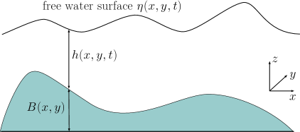
Figure 1: An illustration of the water depth $h$, the bottom topography $B$, and the free water surface level $\eta=h+B$.

We are interested in the preservation of the “lake-at-rest” steady state solution

$$m=hu=0,\quad w=hv=0,\quad\eta=h+B=C$$ (1.3)

where $C$ is a constant. Many physical phenomena can be described as small perturbations of this steady-state solution, including waves on a lake or tsunami waves in the deep ocean. They are difficult, if not impossible, to capture by a numerical method that does not preserve (1.3), on an unrefined mesh. Thus, for the numerical simulation of perturbation waves over the lake-at-rest steady state, it is important to develop schemes that preserve (1.3). These schemes are said in literature to be well-balanced or have the well-balance property or the C-property. Bermudez and Vazquez [3] first introduced a concept of the “exact C-property”. Since then, a number of well-balanced numerical methods have been developed for the SWEs, e.g., finite volume methods [1, 3, 18, 38], finite difference/volume WENO methods [20, 28, 29, 30], and discontinuous Galerkin (DG) methods [9, 10, 19, 27, 29, 30, 31, 32]. DG methods have the advantages of high-order accuracy, high parallel efficiency, and flexibility for $hp$-adaptivity and arbitrary geometry and meshes.

The SWEs exhibit interesting structures including hydraulic jumps/shocks, rarefaction waves, and stationary state transitions. Resolving them in the numerical solution requires fine spatial spacings and thus mesh adaptation becomes a useful tool in improving the computational accuracy and efficiency. Studies have been made in this direction in the past. For example, Tang [26] developed an adaptive moving structured mesh kinetic flux-vector splitting (KFVS) scheme for the SWEs and showed that the method leads to more accurate solutions than methods based on fixed meshes although the well-balance property was not addressed specifically in the work. Lamby et al. [17] proposed an adaptive multi-scale finite volume method for the SWEs with source terms, combining a B-spline based quadtree grid generation strategy and a fully adaptive multi-resolution method. Remacle et al. [23] studied an $h$-adaptive meshing procedure for the transient computation of the SWEs. Zhou et al. [37] proposed a well-balanced adaptive moving mesh generalized Riemann problem (GRP)-based finite volume scheme for the SWEs with irregular bottom topography. Donat et al. [8] developed a well-balanced shock capturing adaptive mesh refinement (AMR) scheme for shallow water flows. Arpaia and Ricchiuto [2] considered several arbitrary Lagrangian-Eulerian (ALE) formulations of the SWEs on moving meshes and provided a discrete analog in the well-balanced finite volume and residual distribution framework. Most recently, a high-order, well-balanced, positivity-preserving and rezoning-type adaptive moving mesh DG method was proposed in [35] for the SWEs. It requires that both the flow variables and bottom topography be updated from the old mesh to the new one at each time step using the same interpolation scheme. A positivity-preserving DG-interpolation scheme [34] has been used in [35] for the purpose.

We consider here a quasi-Lagrange approach of adaptive moving mesh methods where the mesh is considered to move continuously between time steps and interpolation of the flow variables between the old mesh and the new one is unnecessary. The quasi-Lagrange moving mesh DG (QLMM-DG) method has been used successfully for solving hyperbolic conservation laws [21] and the radiative transfer equation [33]. Our focus here is on its application to the SWEs and the well-balance property, and we shall use a change of unknown variables. More specifically, we use the new variables $(\eta=h+B,\,hu,\,hv)$ instead of the original ones $(h,\,hu,\,hv)$ and rewrite the flux (1.2) into a special form (cf. (2.2)) by replacing only some of $h$’s with $\eta$. In the construction of the DG numerical flux, we modify the value of $h$ using the hydrostatic reconstruction technique of [1, 30, 31, 32] but keep $\eta$ unmodified. We will show that the new QLMM-DG method, in both semi-discrete and fully discrete forms, preserves (1.3) while maintaining the high-order accuracy of DG methods. We will also show that a QLMM-DG scheme can be developed based on the SWEs in the original variables but the resulting scheme is well-balanced only in semi-discrete form.

It is worth pointing out that the bottom topography $B$ needs to be updated on the new mesh at each time step in the current method. Nevertheless, unlike the rezoning moving mesh DG method in [35], it places no constraint on the choice of the scheme for updating $B$ to attain the well-balance property. We use $L^{2}$-projection for this purpose in our computation since it is straightforward and economic to implement.

Another challenge in the numerical solution of the SWEs is to preserve the nonnegativity of the water depth in the computation. Following [31, 32], we apply a linear scaling positivity-preserving (PP) limiter [22, 39, 40] to the water depth. However, the PP limiter destroys the well-balance property. To recover the property, we propose to make a high-order correction to the approximation of the bottom topography according to the modifications in the water depth due to the PP limiting. Numerical examples show that this strategy works out well.

For the mesh adaptation, we use a moving mesh PDE (MMPDE) method [12, 13, 14] which is known to produce meshes free of tangling [15]. The MMPDE method uses a metric tensor to determine the size, shape, and orientation of the mesh elements throughout the physical domain. Following [35], we compute the metric tensor based on the equilibrium variable $\mathcal{E}=\frac{1}{2}(u^{2}+v^{2})+g(h+B)$ and the water depth $h$ in the hope that the mesh adapts to the features in the water flow and bottom topography.

An outline of the paper is organized as follows. §2 is devoted to the description of the QLMM-DG method based on the new variables $(\eta,hu,hv)$ and its well-balance property. The discussion of a moving mesh method based on the formulation in the original variables $(h,hu,hv)$ is presented in §3. The generation of an adaptive moving mesh using the MMPDE moving mesh method is described in Appendix A. In §4, a selection of one- and two-dimensional examples are presented and analyzed. Finally, §5 contains the conclusions.

2 The well-balanced QLMM-DG method

In this section we describe the high-order well-balanced positivity-preserving QLMM-DG method for the numerical solution of the SWEs with non-flat bottom topography. This method combines the quasi-Lagrange moving mesh DG method of [21, 33] with the hydrostatic reconstruction technique [1, 30, 32] and a change of unknown variables to attain the well-balance property. The method is described here only in two dimensions. It has a similar form in one dimension.

We use here the new variables $U=(\eta,m,w)^{T}$ instead of the original ones $V=(h,m,w)^{T}$, where $\eta=h+B$. We rewrite the SWEs (1.1) and (1.2) into

$$U_{t}+\nabla\cdot\mathbf{F}(U,h)=S(\eta,B),$$ (2.1)

where

$$\begin{cases}\begin{split}&S(\eta,B)=\big{(}0,-g\eta B_{x},-g\eta B_{y}\big{)}^{T},\\ &\mathbf{F}(U,h)=\begin{bmatrix}[l]m&w\\ \frac{m^{2}}{h}+\frac{1}{2}g(2h\eta-\eta^{2})&\frac{mw}{h}\\ \frac{mw}{h}&\frac{w^{2}}{h}+\frac{1}{2}g(2h\eta-\eta^{2})\\ \end{bmatrix}=\begin{bmatrix}[l]\bm{f}^{1}(U,h)\\ \bm{f}^{2}(U,h)\\ \bm{f}^{3}(U,h)\\ \end{bmatrix}.\end{split}\end{cases}$$ (2.2)

Here, the dependence of $\mathbf{F}$ on $h$ is expressed explicitly although $h$ is a linear function of $\eta$. This is because the value of $h$ will be modified but $\eta$ is kept unmodified in the computation of the numerical flux to attain the well-balance property. Moreover, not all of $h$’s in the flux have been replaced by $\eta-B$, i.e., some are replaced with the new variable $\eta$ and some remain the same. Obviously, there are many of these combinations and thus many forms of the flux; for example, see (2.2 and (2.22). These forms are equal to each other mathematically but can be different numerically. Indeed, we will show that the form (2.2) leads to a well-balanced scheme in both semi-discrete and fully discrete forms while it is unclear if a well-balanced scheme can be obtained from (2.22) (cf. Remark 2.5). We will also show in §3 that a QLMM-DG scheme can be developed based on (1.1) and (1.2) using the original variables but the resulting scheme is well-balanced only in semi-discrete form.

For the moment we assume that a sequence of simplicial meshes having the same number of elements and vertices and the same connectivity, $\mathcal{T}^{0}_{h},\,\mathcal{T}^{1}_{h},\,...$, have been obtained for time instants $t_{0},\,t_{1},\,...$. The generation of these meshes is discussed in Appendix A. Recall that we consider here the quasi-Lagrange approach of moving mesh methods where the mesh is considered to move continuously in time. To this end, for any $n\geq 0$, we define $\mathcal{T}_{h}(t),~{}t\in(t_{n},t_{n+1}]$, as a mesh having the same number of elements and vertices and the same connectivity as $\mathcal{T}_{h}^{n}$ and $\mathcal{T}_{h}^{n+1}$ and having the vertices and nodal velocities given by

$$\begin{split}&\bm{x}_{i}(t)=\frac{t-t_{n}}{\Delta t_{n}}\bm{x}_{i}^{n}+\frac{t_{n+1}-t}{\Delta t_{n}}\bm{x}_{i}^{n+1},\quad i=1,...,N_{v}\\ &\dot{\bm{x}}_{i}=\frac{\bm{x}_{i}^{n+1}-\bm{x}_{i}^{n}}{\Delta t_{n}},\quad i=1,...,N_{v}.\end{split}$$ (2.3)

We also define the piecewise linear mesh velocity function $\dot{\bm{X}}(\bm{x},t)=\big{(}\dot{X},\dot{Y}\big{)}$ as

$$\dot{\bm{X}}(\bm{x},t)=\sum_{i=1}^{N_{v}}\dot{\bm{x}}_{i}\phi_{i}(\bm{x},t),$$ (2.4)

where $\phi_{i}(\bm{x},t)$ is the linear basis function associated with the vertex $\bm{x}_{i}$. For any $K\in\mathcal{T}_{h}(t)$, let $\phi_{K}^{j}(\bm{x},t),~{}j=1,\cdots,n_{b}\equiv(k+1)(k+2)/2$ be the basis functions of the set of polynomials of degree at most $k\geq 1$ on $K$, $P^{k}(K)$. The DG finite element space is defined as

$$\mathcal{V}^{k}_{h}(t)=\{q\in L^{2}(\Omega):\;q|_{K}\in P^{k}(K),\;\forall K\in\mathcal{T}_{h}(t)\}.$$ (2.5)

2.1 The semi-discrete well-balanced QLMM-DG scheme

Multiplying (2.1) with a test function $\phi\in\mathcal{V}^{k}_{h}(t)$, integrating the resulting equation over $K$, and using the Reynolds transport theorem, we have

$$\frac{d}{dt}\int_{K}U\phi d\bm{x}+\int_{K}\phi\nabla\cdot\big{(}-U\dot{\bm{X}}\big{)}d\bm{x}+\int_{K}\phi\nabla\cdot\mathbf{F}(U,h)d\bm{x}=\int_{K}S(\eta,B)\phi d\bm{x}.$$ (2.6)

Recall that we have $h=\eta-B$. Denote

$$\begin{split}\mathbf{H}(U,h)&=\mathbf{F}(U,h)-U\dot{\bm{X}}=\begin{bmatrix}[l]\bm{f}^{1}(U,h)-\eta\dot{\bm{X}}\\ \bm{f}^{2}(U,h)-m\dot{\bm{X}}\\ \bm{f}^{3}(U,h)-w\dot{\bm{X}}\\ \end{bmatrix}.\end{split}$$ (2.7)

From the divergence theorem, we can rewrite (2.6) as

$$\frac{d}{dt}\int_{K}U\phi d\bm{x}-\int_{K}\mathbf{H}(U,h)\cdot\nabla\phi d\bm{x}+\sum_{e_{K}\in\partial K}\int_{e_{K}}\phi\mathbf{H}(U,h)\cdot\bm{n}ds=\int_{K}S(\eta,B)\phi d\bm{x},$$ (2.8)

where $\bm{n}=(n_{x},n_{y})^{T}$ is the outward unit normal to the boundary $\partial K$.

The Jacobian matrix of the vector-valued function $\mathbf{H}\cdot\bm{n}$ with respect to $U$ (with $h$ being considered as a linear function of $\eta$) reads as

$$\begin{bmatrix}[l]-\dot{X}n_{x}-\dot{Y}n_{y}&n_{x}&n_{y}\\ (c^{2}-u^{2})n_{x}-uvn_{y}&(2u-\dot{X})n_{x}+(v-\dot{Y})n_{y}&un_{y}\\ (c^{2}-v^{2})n_{y}-uvn_{x}&vn_{x}&(u-\dot{X})n_{x}+(2v-\dot{Y})n_{y}\\ \end{bmatrix},$$

where $c=\sqrt{gh}$ is the sound speed. The eigenvalues of this matrix can be found as

$$\begin{cases}\begin{split}&\lambda^{1}(U,h,\dot{\bm{X}})=(u-\dot{X})n_{x}+(v-\dot{Y})n_{y}-c,\\ &\lambda^{2}(U,h,\dot{\bm{X}})=(u-\dot{X})n_{x}+(v-\dot{Y})n_{y},\\ &\lambda^{3}(U,h,\dot{\bm{X}})=(u-\dot{X})n_{x}+(v-\dot{Y})n_{y}+c.\end{split}\end{cases}$$ (2.9)

For any variable $q_{h}$ on the boundary $\partial K$, we denote by $q_{h,K}^{int}$ and $q_{h,K}^{ext}$ as the values of $q_{h}$ on $\partial K$ from the interior and exterior of $K$, respectively. We also note that the bottom topography function $B=B(\bm{x})$ needs to be projected into the finite element space $\mathcal{V}_{h}^{k}(t)$ and denote it by $B_{h}$. We use the global Lax-Friedrichs numerical flux to approximate $\mathbf{H}(U,h)\cdot\bm{n}^{e}_{K}$ for $\bm{x}\in e_{K}\subset\partial K$, i.e.,

$$\begin{split}\hat{\mathbf{H}}|_{e_{K}}&=\hat{\mathbf{H}}(U_{h,K}^{int},h_{h,K}^{int};U_{h,K}^{ext},h_{h,K}^{ext};\bm{n}^{e}_{K})\\ &=\frac{1}{2}\Big{(}\big{(}\mathbf{H}(U_{h,K}^{int},h_{h,K}^{int})+\mathbf{H}(U_{h,K}^{ext},h_{h,K}^{ext})\big{)}\cdot\bm{n}_{K}-\alpha_{h}(U_{h,K}^{ext}-U_{h,K}^{int})\Big{)},\end{split}$$ (2.10)

where $h_{h,K}^{int}=\eta_{h,K}^{int}-B_{h,K}^{int}$, $h_{h,K}^{ext}=\eta_{h,K}^{ext}-B_{h,K}^{ext}$, and

$$\alpha_{h}=\max\limits_{K,e_{K},m}\left(\max\limits\Big{(}|\lambda^{m}(U_{h,K}^{int},h_{h,K}^{int},\dot{\bm{X}}|_{e_{K}})|,\;|\lambda^{m}(U_{h,K}^{ext},h_{h,K}^{ext},\dot{\bm{X}}|_{e_{K}})|\Big{)}\right).$$

We can then define a semi-discrete DG approximation $U_{h}\in\mathcal{V}^{k}_{h}(t)$ for (2.1) such that

$$\begin{split}&\frac{d}{dt}\int_{K}U_{h}\phi d\bm{x}-\int_{K}\mathbf{H}(U_{h},h_{h})\cdot\nabla\phi d\bm{x}+\sum_{e_{K}\in\partial K}\int_{e_{K}}\phi\hat{\mathbf{H}}|_{e_{K}}ds\\ &~{}~{}~{}~{}~{}~{}~{}~{}~{}~{}~{}~{}~{}~{}~{}~{}~{}~{}=\int_{K}S(\eta_{h},B_{h})\phi d\bm{x},\quad\forall\phi\in\mathcal{V}^{k}_{h}(t),\quad\forall K\in\mathcal{T}_{h}(t),\end{split}$$ (2.11)

where $h_{h}=\eta_{h}-B_{h}$. In actual computation, the area and line integrals in the above equation are calculated using Gaussian quadrature rules. Define the residual associated with this scheme as

$$\begin{split}R_{h,K}(t)=&\frac{d}{dt}\int_{K}U_{h}\phi d\bm{x}-\int_{K}\phi\nabla\cdot(U_{h}\dot{\bm{X}})d\bm{x}\\ =&\int_{K}S(\eta_{h},B_{h})\phi d\bm{x}+\int_{K}\mathbf{H}(U_{h},h_{h})\cdot\nabla\phi d\bm{x}\\ &-\sum_{e_{K}\in\partial K}\int_{e_{K}}\phi\hat{\mathbf{H}}|_{e_{K}}ds-\int_{K}\phi\nabla\cdot(U_{h}\dot{\bm{X}})d\bm{x},\quad\forall K\in\mathcal{T}_{h}(t).\end{split}$$ (2.12)

Note that a term is added in the definition to account for the effects of mesh movement. It is not difficult to show that (1.3) is preserved if this residual vanishes for the lake-at-rest steady state. Unfortunately, it can be verified that the latter does not hold in general and thus the scheme (2.11) is not well-balanced. The main issue is that the numerical flux $\hat{\mathbf{H}}|_{e_{K}}$ does not reduce to $\mathbf{H}\big{(}U_{h,K}^{int},h_{h,K}^{int}\big{)}\cdot\bm{n}_{K}^{e}$ for the lake-at-rest steady state and the line integrals cannot be converted back into an area integral involving $\mathbf{H}$ under the divergence theorem.

To attain the well-balance property, we use the hydrostatic reconstruction technique of [1, 30, 32] to construct a new numerical flux $\hat{\mathbf{H}}^{*}|_{e_{K}}$ from $\hat{\mathbf{H}}|_{e_{K}}$. To this end, we first compute

$$\begin{cases}\begin{split}&h_{h,K}^{*,int}|_{e_{K}}=\max\Big{(}0,\eta_{h,K}^{int}|_{e_{K}}-\max\big{(}B_{h,K}^{int}|_{e_{K}},B_{h,K}^{ext}|_{e_{K}}\big{)}\Big{)},\\ &h_{h,K}^{*,ext}|_{e_{K}}=\max\Big{(}0,\eta_{h,K}^{ext}|_{e_{K}}-\max\big{(}B_{h,K}^{int}|_{e_{K}},B_{h,K}^{ext}|_{e_{K}}\big{)}\Big{)}.\end{split}\end{cases}$$ (2.13)

Notice that the value of $B_{h}$ on $e_{K}$ is taken as $\max\big{(}B_{h,K}^{int}|_{e_{K}},B_{h,K}^{ext}|_{e_{K}}\big{)}$. Moreover, $h_{h,K}^{*,int}|_{e_{K}}$ and $h_{h,K}^{*,ext}|_{e_{K}}$ are chosen to guarantee $h_{h,K}^{*,int}|_{e_{K}}\geq 0$ and $h_{h,K}^{*,ext}|_{e_{K}}\geq 0$ while trying to satisfy

$$\begin{cases}\begin{split}&h_{h,K}^{*,int}+\max\big{(}B_{h,K}^{int}|_{e_{K}},B_{h,K}^{ext}|_{e_{K}}\big{)}=\eta_{h,K}^{int}|_{e_{K}},\\ &h_{h,K}^{*,ext}+\max\big{(}B_{h,K}^{int}|_{e_{K}},B_{h,K}^{ext}|_{e_{K}}\big{)}=\eta_{h,K}^{ext}|_{e_{K}}.\end{split}\end{cases}$$

Then, the interior and exterior values of $U=(\eta,m,w)^{T}$ are modified as

$$\begin{cases}\begin{split}&\eta_{h,K}^{*,int}=\eta_{h,K}^{int},\qquad\qquad\eta_{h,K}^{*,ext}=\eta_{h,K}^{ext},\\ &m_{h,K}^{*,int}=\frac{h_{h,K}^{*,int}}{h_{h,K}^{int}}m_{h,K}^{int},\quad m_{h,K}^{*,ext}=\frac{h_{h,K}^{*,ext}}{h_{h,K}^{ext}}m_{h,K}^{ext},\\ &w_{h,K}^{*,int}=\frac{h_{h,K}^{*,int}}{h_{h,K}^{int}}w_{h,K}^{int},\quad w_{h,K}^{*,ext}=\frac{h_{h,K}^{*,ext}}{h_{h,K}^{ext}}w_{h,K}^{ext}.\end{split}\end{cases}$$ (2.14)

It is worth pointing out that the value of $h$ has been modified but that of $\eta$ remains unmodified. Finally, the new flux $\hat{\mathbf{H}}^{*}$ on the edge $e_{K}\in\partial K$ is given by

$$\hat{\mathbf{H}}^{*}|_{e_{K}}=\hat{\mathbf{H}}(U_{h,K}^{*,int},h_{h,K}^{*,int};U_{h,K}^{*,ext},h_{h,K}^{*,ext};\bm{n}^{e}_{K})+\Delta^{*}_{e_{K}}\cdot\bm{n}_{K}^{e},$$ (2.15)

where

$$\Delta^{*}_{e_{K}}=\begin{bmatrix}[l]0&0\\ g\eta_{h,K}^{int}|_{e_{K}}\big{(}h_{h,K}^{int}|_{e_{K}}-h_{h,K}^{*,int}|_{e_{K}}\big{)}&0\\ 0&g\eta_{h,K}^{int}|_{e_{K}}\big{(}h_{h,K}^{int}|_{e_{K}}-h_{h,K}^{*,int}|_{e_{K}}\big{)}\\ \end{bmatrix}.$$ (2.16)

The correction term is chosen to satisfy (2.17) below.

Lemma 2.1

For the lake-at-rest steady state, the numerical flux $\hat{\mathbf{H}}^{*}|_{e_{K}}$ defined in (2.15) and (2.16) satisfies

$$\hat{\mathbf{H}}^{*}|_{e_{K}}=\mathbf{H}\big{(}U_{h,K}^{int},h_{h,K}^{int}\big{)}\cdot\bm{n}_{K}^{e}.$$ (2.17)

Proof 2.2

For the lake-at-rest steady state $(\eta_{h},m_{h},w_{h})=(C,0,0)$, where $C$ is a constant, we have

$$\eta_{h,K}^{int}|_{e_{K}}=\eta_{h,K}^{ext}|_{e_{K}}=C,\quad m_{h,K}^{int}|_{e_{K}}=m_{h,K}^{ext}|_{e_{K}}=0,\quad w_{h,K}^{int}|_{e_{K}}=w_{h,K}^{ext}|_{e_{K}}=0.$$

From the definition (2.13) and (2.14), we have

$$h_{h,K}^{*,int}|_{e_{K}}=h_{h,K}^{*,ext}|_{e_{K}},\quad U_{h,K}^{*,int}|_{e_{K}}=U_{h,K}^{*,ext}|_{e_{K}},$$

$$\eta_{h,K}^{*,int}|_{e_{K}}=\eta_{h,K}^{*,ext}|_{e_{K}}=C,\quad m_{h,K}^{*,int}|_{e_{K}}=m_{h,K}^{*,ext}|_{e_{K}}=0,\quad w_{h,K}^{*,int}|_{e_{K}}=w_{h,K}^{*,ext}|_{e_{K}}=0.$$

Using these and the consistency of the numerical flux, from (2.2) and (2.15) we have

$$\begin{split}\hat{\mathbf{H}}^{*}|_{e_{K}}&=\hat{\mathbf{H}}(U_{h,K}^{*,int},h_{h,K}^{*,int};U_{h,K}^{*,ext},h_{h,K}^{*,ext};\bm{n}^{e}_{K})+\Delta^{*}_{e_{K}}\cdot\bm{n}_{K}^{e}\\ &=\mathbf{H}\big{(}U_{h,K}^{*,int},h_{h,K}^{*,int}\big{)}\cdot\bm{n}_{K}^{e}+\Delta^{*}_{e_{K}}\cdot\bm{n}_{K}^{e}\\ &=\begin{bmatrix}[l]-\big{(}\dot{X}\eta_{h,K}^{*,int}\big{)}\big{|}_{e_{K}}&-\big{(}\dot{Y}\eta_{h,K}^{*,int}\big{)}\big{|}_{e_{K}}\\ \frac{g}{2}\Big{(}2\eta_{h,K}^{*,int}h_{h,K}^{*,int}-\big{(}\eta_{h,K}^{*,int}\big{)}^{2}\Big{)}\Big{|}_{e_{K}}&0\\ 0&\frac{g}{2}\Big{(}2\eta_{h,K}^{*,int}h_{h,K}^{*,int}-\big{(}\eta_{h,K}^{*,int}\big{)}^{2}\Big{)}\Big{|}_{e_{K}}\end{bmatrix}\cdot\bm{n}_{K}^{e}\\ &+\begin{bmatrix}[l]0&0\\ \big{(}g\eta_{h,K}^{int}(h_{h,K}^{int}-h_{h,K}^{*,int})\big{)}\big{|}_{e_{K}}&0\\ 0&\big{(}g\eta_{h,K}^{int}(h_{h,K}^{int}-h_{h,K}^{*,int})\big{)}\big{|}_{e_{K}}\\ \end{bmatrix}\cdot\bm{n}_{K}^{e}\\ &=\begin{bmatrix}[l]-\big{(}\dot{X}\eta_{h,K}^{int}\big{)}\big{|}_{e_{K}}&-\big{(}\dot{Y}\eta_{h,K}^{int}\big{)}\big{|}_{e_{K}}\\ \frac{g}{2}\Big{(}2\eta_{h,K}^{int}h_{h,K}^{int}-\big{(}\eta_{h,K}^{int}\big{)}^{2}\Big{)}\Big{|}_{e_{K}}&0\\ 0&\frac{g}{2}\Big{(}2\eta_{h,K}^{int}h_{h,K}^{int}-\big{(}\eta_{h,K}^{int}\big{)}^{2}\Big{)}\Big{|}_{e_{K}}\end{bmatrix}\cdot\bm{n}_{K}^{e}\\ &=\mathbf{H}\big{(}U_{h,K}^{int},h_{h,K}^{int}\big{)}\cdot\bm{n}_{K}^{e}.\end{split}$$

Replacing $\hat{\mathbf{H}}|_{e_{K}}$ by $\hat{\mathbf{H}}^{*}|_{e_{K}}$ in (2.11), we obtain the semi-discrete QLMM-DG scheme, i.e., to find $U_{h}\in\mathcal{V}^{k}_{h}(t)$ such that

$$\begin{split}&\frac{d}{dt}\int_{K}U_{h}\phi d\bm{x}-\int_{K}\mathbf{H}(U_{h},h_{h})\cdot\nabla\phi d\bm{x}+\sum_{e_{K}\in\partial K}\int_{e_{K}}\phi\hat{\mathbf{H}}^{*}|_{e_{K}}ds\\ &~{}~{}~{}~{}~{}~{}~{}~{}~{}~{}~{}~{}~{}~{}~{}~{}~{}~{}~{}~{}~{}~{}~{}~{}=\int_{K}S(\eta_{h},B_{h})\phi d\bm{x},\quad\forall\phi\in\mathcal{V}^{k}_{h}(t),\quad\forall K\in\mathcal{T}_{h}(t)\end{split}$$ (2.18)

where $h_{h}=\eta_{h}-B_{h}$. Denote the residual for this scheme as

$$\begin{split}R^{*}_{h,K}(t)=&R^{*}(U_{h},h_{h},\phi,B_{h})|_{K}\\ =&\int_{K}S(\eta_{h},B_{h})\phi d\bm{x}+\int_{K}\mathbf{H}(U_{h},h_{h})\nabla\phi d\bm{x}\\ &-\sum_{e_{K}\in\partial K}\int_{e_{K}}\phi\hat{\mathbf{H}}^{*}|_{e_{K}}ds-\int_{K}\phi\nabla\cdot(U_{h}\dot{\bm{X}})d\bm{x}.\end{split}$$ (2.19)

Proposition 2.3

If all integrals in (2.19) are computed exactly (with suitable Gaussian quadrature rules), the residual of the semi-discrete QLMM-DG scheme (2.18) with the numerical flux (2.15) and (2.16) vanishes for the lake-at-rest steady state and thus the scheme (2.18) is well-balanced.

Proof 2.4

For the lake-at-rest steady state $(\eta_{h},m_{h},w_{h})=(C,0,0)$, using the Lemma 2.1, the divergence theorem, and the definition (2.7), we have, for any $K\in\mathcal{T}_{h}(t)$ and any $\phi\in\mathcal{V}^{k}_{h}(t)$,

$$\begin{split}R^{*}_{h,K}(t)=&\int_{K}S(\eta_{h},B_{h})\phi d\bm{x}-\int_{K}\phi\nabla\cdot(U_{h}\dot{\bm{X}})d\bm{x}\\ &-\sum_{e_{K}\in\partial K}\int_{e_{K}}\phi\hat{\mathbf{H}}^{*}|_{e_{K}}ds+\int_{K}\mathbf{H}(U_{h},h_{h})\cdot\nabla\phi d\bm{x}\\ =&\int_{K}S(\eta_{h},B_{h})\phi d\bm{x}-\int_{K}\phi\nabla\cdot(U_{h}\dot{\bm{X}})d\bm{x}\\ &-\sum_{e_{K}\in\partial K}\int_{e_{K}}\phi\mathbf{H}\big{(}U_{h,K}^{int},h_{h,K}^{int}\big{)}\cdot\bm{n}_{K}^{e}ds+\int_{K}\mathbf{H}(U_{h},h_{h})\cdot\nabla\phi d\bm{x}\\ =&\int_{K}S(\eta_{h},B_{h})\phi d\bm{x}-\int_{K}\phi\nabla\cdot\big{(}\mathbf{H}(U_{h},h_{h})+U_{h}\dot{\bm{X}}\big{)}d\bm{x}\\ =&\int_{K}\big{(}S(\eta_{h},B_{h})-\nabla\cdot\mathbf{F}(U_{h},h_{h})\big{)}\phi d\bm{x}=0.\end{split}$$

To see the convergence order of the scheme, we rewrite (2.18) into

$$\frac{d}{dt}\int_{K}U_{h}\phi d\bm{x}+\sum_{e_{K}\in\partial K}\int_{e_{K}}\phi\hat{\mathbf{H}}|_{e_{K}}ds-\int_{K}\mathbf{H}(U_{h},h_{h})\cdot\nabla\phi d\bm{x}$$

$$\qquad\qquad=\int_{K}S(h_{h},B_{h})\phi d\bm{x}+\sum_{e_{K}\in\partial K}\int_{e_{K}}\phi\big{(}\hat{\mathbf{H}}^{*}-\hat{\mathbf{H}}\big{)}|_{e_{K}}ds,\quad\forall\phi\in\mathcal{V}^{k}_{h}(t).$$ (2.20)

This is a standard DG scheme for (2.1) on a moving mesh with a correction term (the last term). Notice that

$$\begin{split}\big{|}\eta_{h,K}^{int}|_{e_{K}}\big{(}h_{h,K}^{int}|_{e_{K}}-h_{h,K}^{*,int}|_{e_{K}}\big{)}\big{|}&\leq\big{|}\eta_{h,K}^{int}|_{e_{K}}\big{|}\cdot\big{|}\big{(}h_{h,K}^{int}-h_{h,K}^{*,int}\big{)}|_{e_{K}}\big{|}=\mathcal{O}(a^{k+1}_{max}),\end{split}$$

where $a_{max}$ denotes the maximum element diameter of the mesh. This gives $\hat{\mathbf{H}}^{*}-\hat{\mathbf{H}}=\mathcal{O}(a^{k+1}_{max})$. Thus, the scheme (2.18) is $(k+1)$-th-order in space.

Remark 2.5

As mentioned earlier, we can replace all of $h$’s in the flux by $\eta-B$. This gives the system [16]

$$U_{t}+\nabla\cdot\mathbb{F}(U,B)=S(\eta,B),$$ (2.21)

where

$$\begin{split}&\mathbb{F}(U,B)=\begin{bmatrix}[l]m&w\\ \frac{m^{2}}{\eta-B}+\frac{1}{2}g(\eta^{2}-2\eta B)&\frac{mw}{\eta-B}\\ \frac{mw}{\eta-B}&\frac{w^{2}}{\eta-B}+\frac{1}{2}g(\eta^{2}-2\eta B)\\ \end{bmatrix}.\end{split}$$ (2.22)

Applying the same procedure to this system, we can obtain a QLMM-DG scheme. For the lake-at-rest steady state, for this scheme we have

$$\eta_{h,K}^{int}|_{e_{K}}=\eta_{h,K}^{ext}|_{e_{K}}=C,\quad m_{h,K}^{int}|_{e_{K}}=m_{h,K}^{ext}|_{e_{K}}=0,\quad w_{h,K}^{int}|_{e_{K}}=w_{h,K}^{ext}|_{e_{K}}=0,$$

and $U_{h,K}^{int}|_{e_{K}}=U_{h,K}^{ext}|_{e_{K}}$. However, since $\mathbb{F}(U,B)$ involves $B$ explicitly and since $B_{h,K}^{int}|_{e_{K}}$ is not equal to $B_{h,K}^{ext}|_{e_{K}}$ in general, it is unclear how the numerical flux can be modified to ensure (2.17). Hence, it remains unknown if a well-balanced QLMM-DG scheme can be developed based on (2.21).

2.2 The fully discrete well-balanced QLMM-DG scheme

We consider the third-order explicit total variation diminishing (TVD) Runge-Kutta scheme to discretize (2.18) in time. For notational simplicity, we denote

$$\begin{split}\mathcal{L}(U_{h},h_{h},\phi,B_{h})|_{K}&=-\sum_{e_{K}\in\partial K}\int_{e_{K}}\phi\hat{\mathbf{H}}^{*}|_{e_{K}}ds+\int_{K}\mathbf{H}(U_{h},h_{h})\cdot\nabla\phi d\bm{x}\\ &\qquad+\int_{K}S(\eta_{h},B_{h})\phi d\bm{x}.\end{split}$$ (2.23)

We can rewrite (2.18) into a compact form as

$$\frac{d}{dt}\int_{K}U_{h}\phi d\bm{x}=\mathcal{L}(U_{h},h_{h},\phi,B_{h})|_{K},\quad\forall\phi\in\mathcal{V}_{h}^{k}(t).$$ (2.24)

Applying the third-order explicit TVD Runge-Kutta scheme to the above equation, we obtain the fully-discrete QLMM-DG scheme as

$$\begin{cases}\begin{split}\int_{K^{n,(1)}}U_{h}^{n,(1)}\phi^{n,(1)}d\bm{x}&=\int_{K^{n}}U_{h}^{n}\phi^{n}d\bm{x}+\Delta t_{n}\mathcal{L}(U_{h}^{n},h_{h}^{n},\phi^{n},B_{h}^{n})|_{K^{n}},\\ \int_{K^{n,(2)}}U_{h}^{n,(2)}\phi^{n,(2)}d\bm{x}&=\frac{3}{4}\int_{K^{n}}U_{h}^{n}\phi^{n}d\bm{x}+\frac{1}{4}\int_{K^{n,(1)}}U_{h}^{n,(1)}\phi^{n,(1)}d\bm{x}\\ &~{}~{}~{}~{}~{}~{}~{}~{}~{}~{}~{}~{}~{}+\frac{1}{4}\Delta t_{n}\mathcal{L}(U_{h}^{n,(1)},h_{h}^{n,(1)},\phi^{n,(1)},B^{n,(1)}_{h})|_{K^{n,(1)}},\\ \int_{K^{n+1}}U_{h}^{n+1}\phi^{n+1}d\bm{x}&=\frac{1}{3}\int_{K^{n}}U_{h}^{n}\phi^{n}d\bm{x}+\frac{2}{3}\int_{K^{n,(2)}}U_{h}^{n,(2)}\phi^{n,(2)}d\bm{x}\\ &~{}~{}~{}~{}~{}~{}~{}~{}~{}~{}~{}~{}~{}+\frac{2}{3}\Delta t_{n}\mathcal{L}(U_{h}^{(2)},h_{h}^{n,(2)},\phi^{n,(2)},B^{n,(2)}_{h})|_{K^{n,(2)}},\end{split}\end{cases}$$ (2.25)

where $U_{h}^{n,(1)}$, $h_{h}^{n,(1)}$, $\phi^{n,(1)}$, $B_{h}^{n,(1)}$, $K^{n,(1)}$ are stage values at $t=t_{n}+\Delta t_{n}$, $U_{h}^{n,(2)}$, $h_{h}^{n,(2)}$, $\phi^{n,(2)}$, $B_{h}^{n,(2)}$, $K^{n,(2)}$ are the values at $t=t_{n}+\frac{1}{2}\Delta t_{n}$, and $U_{h}^{n+1}$, $h_{h}^{n+1}$, $\phi^{n+1}$, $K^{n+1}$ are at $t=t_{n}+\Delta t_{n}$.

We now make a few remarks on the above scheme. We first note that $h_{h}$ is updated by

$$h_{h}^{n,(1)}=\eta_{h}^{n,(1)}-B_{h}^{n,(1)},\quad h_{h}^{n,(2)}=\eta_{h}^{n,(2)}-B_{h}^{n,(2)},\quad h_{h}^{n+1}=\eta_{h}^{n+1}-B_{h}^{n+1}.$$

Second, let $\hat{K}$ be the reference element and $\hat{\phi}=\hat{\phi}(\bm{\xi})$ be an arbitrary basis function. Then, the test functions in (2.25) corresponding to this basis function are related by

$$\phi^{n}(\bm{x})=\hat{\phi}(F^{-1}_{K^{n}}(\bm{x})),\quad\phi^{n,(1)}(\bm{x})=\hat{\phi}(F^{-1}_{K^{n,(1)}}(\bm{x})),$$

$$\phi^{n,(2)}(\bm{x})=\hat{\phi}(F^{-1}_{K^{n,(2)}}(\bm{x})),\quad\phi^{n+1}(\bm{x})=\hat{\phi}(F^{-1}_{K^{n+1}}(\bm{x})),$$

where $F^{-1}_{K}$ is the inverse of the affine mapping $F_{K}:\hat{K}\to K$ with $K$ being $K^{n}$, $K^{n,(1)}$, $K^{n,(2)}$, or $K^{n+1}$.

Third, the area of $K^{n,(1)}$, $K^{n,(2)}$ and $K^{n+1}$ is needed in the computation of the integrals in (2.25). It can be calculated using the coordinates of the vertices of the elements. But this does not preserve the so-called geometric conservation law (GCL) that is a geometric identity in the continuous setting. Using the Reynolds transport theorem and the divergence theorem, we can find the GCL as

$$\frac{d}{dt}\int_{K}d\bm{x}=\int_{\partial K}\dot{\bm{X}}\cdot\bm{n}ds\quad\mbox{ or }\quad\frac{d}{dt}\int_{K}d\bm{x}=\int_{K}\nabla\cdot\dot{\bm{X}}d\bm{x}.$$ (2.26)

Since $\dot{\bm{X}}$ is a linear function in $K$ and $\nabla\cdot\dot{\bm{X}}$ is constant, we get

$$\frac{d}{dt}|K|=|K|\nabla\cdot\dot{\bm{X}}|_{K}.$$ (2.27)

Applying the third-order Runge-Kutta scheme to the above equation, we have

$$\begin{cases}\begin{split}|K^{n,(1)}|&=|K^{n}|+\Delta t_{n}|K^{n}|\nabla\cdot\dot{\bm{X}}^{n}_{K^{n}},\\ |K^{n,(2)}|&=\frac{3}{4}|K^{n}|+\frac{1}{4}\big{(}|K^{n,(1)}|+\Delta t_{n}|K^{n,(1)}|\nabla\cdot\dot{\bm{X}}^{n,(1)}_{K^{n,(1)}}\big{)},\\ |K^{n+1}|&=\frac{1}{3}|K^{n}|+\frac{2}{3}\big{(}|K^{n,(2)}|+\Delta t_{n}|K^{n,(2)}|\nabla\cdot\dot{\bm{X}}^{n,(2)}_{K^{n,(2)}}\big{)}.\end{split}\end{cases}$$ (2.28)

Thus, the area of $K^{n,(1)}$, $K^{n,(2)}$ and $K^{n+1}$ can be updated using this equation. We note that a factor involving the area of the element appears in the computation of $\nabla\cdot\dot{\bm{X}}^{n,(1)}_{K^{n,(1)}}$ and $\nabla\cdot\dot{\bm{X}}^{n,(2)}_{K^{n,(2)}}$ and this factor should be computed using $|K^{n,(1)}|$ and $|K^{n,(2)}|$ (i.e., the values obtained through the above equation instead of those directly computed using the coordinates of the element vertices), respectively. The preservation of GCL has been studied extensively in the context of moving mesh computation; e.g., see Trulio and Trigger [25] and Thomas and Lombard [24]. As will be seen in Proposition 2.6, updating the area of elements using (2.28) is an important step for the QLMM-DG scheme (2.25) to be well-balanced.

It is interesting to point out that $|K^{n+1}|$ calculated through (2.28) is the same as that directly computed using the vertex coordinates of $K^{n+1}$. (The other stage values $|K^{n,(1)}|$ and $|K^{n,(2)}|$ are different from their counterparts in general.) Indeed, this property holds for the third-order Runge-Kutta scheme in one, two, and three dimensions. The validity of this property depends on the time integration scheme used and the dimensionality of the space. For example, it holds only in one dimension when the forward Euler scheme is used. In case when $|K^{n+1}|$ calculated through the GCL update is not equal to that computed using the vertex coordinates, we suggest to start the GCL update with $|K^{n}|$ calculated from the vertex coordinates. This does not affect the satisfaction of GCL.

Fourth, we emphasize that the update of $B$ does not affect the well-balance property of the QLMM-DG scheme. For this reason, in our computation we use $L^{2}$-projection to compute $B_{h}^{n,(1)}$, $B_{h}^{n,(2)}$, and $B_{h}^{n+1}$. Since $B$ is a given function, $L^{2}$-projection is straightforward and economic to implement.

It is interesting to point out that the requirements for how $B$ is updated are different in the current QLMM-DG method and the rezoning-type moving mesh DG method of [35]. The latter requires that the same scheme be used to update both the bottom topography and flow variables. It is shown there that a DG-interpolation scheme works out well for this purpose but $L^{2}$-projection may be difficult to use. This is because, when it is used for $B$, then $L^{2}$-projection needs to be used for the flow variables as well. Since only numerical approximations are available for the flow variables, their $L^{2}$-projection from the old mesh to the new one requires finding the intersection between elements in the new and old meshes and performing numerical integration thereon, which is known to be a difficult, if not impossible, task in programming.

Fifth, the DG solution of the SWEs may contain spurious oscillations and even nonlinear instability. We need to apply a nonlinear limiter after each Runge-Kutta stage to aviod those spurious oscillations. However, caution must be taken since this limiting procedure can destroy the well-balance property. Following [1, 30, 38], we use the TVB limiter [4, 5, 6] for the local characteristic variables based on the variables $\big{(}\eta,m,w\big{)}$. This procedure is known to preserve the lake-at-rest steady state and conserve the cell averages.

Sixth, another challenge in the numerical solution of the SWEs is to preserve the nonnegativity of the water depth $h$ in the computation. Following [31, 32], we can show that, after each Runge-Kutta stage of the scheme (2.25), the cell averages of the current approximation of $h$ are nonnegative if the cell averages and the function values of the previous approximation of $h$ at a set of special quadrature points (Gauss-Lobatto quadrature points in one dimension) [32] for each mesh element are nonnegative. Since the TVB limiter preserves the cell averages, we can use the linear scaling PP limiter [22, 39, 40] to ensure the nonnegativity of $h$ after each application of the TVB limiter.

However, the PP limiter destroys the well-balance property. To restore the property, we make a high-order correction to the current approximation of the bottom topography according to the modifications in the water depth due to the PP limiting, i.e.,

$$\hat{B}_{h}=B_{h}-(\hat{h}_{h}-h_{h}),$$ (2.29)

where $\hat{h}_{h}$ denotes the modification of $h_{h}$ by the PP limiter. It is known that [22, 39, 40] this PP limiter maintains the cell averages and high-order accuracy, i.e., $\overline{\hat{h}_{K}}=\overline{h_{K}}$, for all elements $K$ and $\hat{h}_{h}-h_{h}=\mathcal{O}(a_{max}^{k+1})$, where $a_{max}$ is the maximum element diameter of the mesh. Thus, $\hat{B}_{h}$ has the same cell averages as $B_{h}$.

It is worth pointing out that the above trick has been used successfully in the rezoning-type moving mesh DG method [35] to restore the well-balance property.

Finally, to ensure the stability of the method, the time step for (2.25) is chosen subject to the Courant-Friedrichs-Lewy (CFL) condition [7]. For a fixed mesh, the time step is taken as

$$\Delta t_{n,1}\leq\frac{C_{cfl}}{\max\limits_{K,e}\Big{(}\max\limits_{m}|\tilde{\lambda}^{m}(U_{h}^{n},h_{h}^{n})|\Big{)}}\cdot a^{n}_{min},$$ (2.30)

where $C_{cfl}$ is a constant typically chosen to be less than $1/(2k+1)$, $a^{n}_{min}$ is the minimum height of the elements of $\mathcal{T}_{h}^{n}$, and $\tilde{\lambda}^{m}(U,h)$, $m=1,\,2,\,3$ denote the eigenvalues of $\mathbf{F}^{\prime}(U,h)\cdot\bm{n}_{K}$, i.e.,

$$\tilde{\lambda}^{1}(U,h)=un_{x}+vn_{y}-c,\quad\tilde{\lambda}^{2}(U,h)=un_{x}+vn_{y},\quad\tilde{\lambda}^{3}(U,h)=un_{x}+vn_{y}+c.$$

For a moving mesh, we need to consider the extra convection term caused by mesh movement and thus take the time step as

$$\Delta t_{n,2}\leq\frac{C_{cfl}}{\max\limits_{K,e}\Big{(}\max\limits_{m}|\lambda^{m}(U_{h}^{n},h_{h}^{n},\dot{\bm{X}}^{n})|\Big{)}}\cdot\min\big{(}a^{n}_{min},a^{n+1}_{min}),$$ (2.31)

where $\lambda^{m},~{}m=1,2,3$ are defined in (2.9). Finally, we take $\Delta t_{n}=\min\big{(}\Delta t_{n,1},\Delta t_{n,2}\big{)}$.

Next, we show that the fully discrete QLMM-DG scheme (2.25) is well-balanced in the following proposition.

Proposition 2.6

If the area of mesh elements is updated according to (2.28) and all integrals in (2.23) are computed exactly, then the fully discrete QLMM-DG scheme (2.25) preserves the lake-at-rest steady-state solutions, i.e., $\eta^{n}_{h}=C$, $m^{n}_{h}=0$, and $w^{n}_{h}=0$ imply $\eta^{n+1}_{h}=C$, $m^{n+1}_{h}=0$, and $w^{n+1}_{h}=0$, where $C$ is a constant.

Proof 2.7

Recall that $R^{*}(U_{h},h_{h},\phi,B_{h})|_{K}$ vanishes for the lake-at-rest steady state. Comparing the expressions of $\mathcal{L}(U_{h},h_{h},\phi,B_{h})|_{K}$ in (2.23) and $R^{*}(U_{h},h_{h},\phi,B_{h})|_{K}$ in (2.19), we have

$$\mathcal{L}(U_{h},h_{h},\phi,B_{h})|_{K}=R^{*}(U_{h},h_{h},\phi,B_{h})|_{K}+\int_{K}\phi\nabla\cdot(U_{h}\dot{\bm{X}})d\bm{x}.$$

Then (2.25) becomes

$$\begin{split}\int_{K^{n,(1)}}U_{h}^{n,(1)}\phi^{n,(1)}d\bm{x}&=\int_{K^{n}}U_{h}^{n}\phi^{n}d\bm{x}+\Delta t_{n}\int_{K^{n}}\phi^{n}\nabla\cdot\big{(}U^{n}_{h}\dot{\bm{X}}^{n}\big{)}d\bm{x},\\ \int_{K^{n,(2)}}U_{h}^{n,(2)}\phi^{n,(2)}d\bm{x}&=\frac{3}{4}\int_{K^{n}}U_{h}^{n}\phi^{n}d\bm{x}+\frac{1}{4}\int_{K^{n,(1)}}U_{h}^{n,(1)}\phi^{n,(1)}d\bm{x}\\ &~{}~{}~{}~{}~{}~{}~{}~{}~{}~{}~{}~{}~{}~{}~{}~{}~{}~{}~{}~{}~{}~{}~{}+\frac{1}{4}\Delta t_{n}\int_{K^{n,(1)}}\phi^{n,(1)}\nabla\cdot\big{(}U^{n,(1)}_{h}\dot{\bm{X}}^{n,(1)}\big{)}d\bm{x},\\ \int_{K^{n+1}}U_{h}^{n+1}\phi^{n+1}d\bm{x}&=\frac{1}{3}\int_{K^{n}}U_{h}^{n}\phi^{n}d\bm{x}+\frac{2}{3}\int_{K^{n,(2)}}U_{h}^{n,(2)}\phi^{n,(2)}d\bm{x}\\ &~{}~{}~{}~{}~{}~{}~{}~{}~{}~{}~{}~{}~{}~{}~{}~{}~{}~{}~{}~{}~{}~{}~{}+\frac{2}{3}\Delta t_{n}\int_{K^{n,(2)}}\phi^{n,(2)}\nabla\cdot\big{(}U^{n,(2)}_{h}\dot{\bm{X}}^{n,(2)}\big{)}d\bm{x}.\end{split}$$

It is not difficult to show from the above equations that $m^{n+1}_{h}=0$ and $w^{n+1}_{h}=0$ if $m^{n}_{h}=0$ and $w^{n}_{h}=0$. We rewrite the first component of the above equations as

$$\begin{split}\int_{K^{n,(1)}}\eta_{h}^{n,(1)}\phi^{n,(1)}d\bm{x}=&~{}~{}\int_{K^{n}}\eta_{h}^{n}\phi^{n}d\bm{x}+\Delta t_{n}\int_{K^{n}}\phi^{n}\nabla\cdot\big{(}\eta^{n}_{h}\dot{\bm{X}}^{n}\big{)}d\bm{x},\\ \int_{K^{n,(2)}}\eta_{h}^{n,(2)}\phi^{n,(2)}d\bm{x}=&\frac{3}{4}\int_{K^{n}}\eta_{h}^{n}\phi^{n}d\bm{x}+\frac{1}{4}\int_{K^{n,(1)}}\eta_{h}^{n,(1)}\phi^{n,(1)}d\bm{x}\\ &~{}~{}~{}~{}~{}~{}~{}~{}~{}~{}~{}~{}~{}~{}~{}~{}~{}~{}+\frac{1}{4}\Delta t_{n}\int_{K^{n,(1)}}\phi^{n,(1)}\nabla\cdot\big{(}\eta^{n,(1)}_{h}\dot{\bm{X}}^{n,(1)}\big{)}d\bm{x},\\ \int_{K^{n+1}}\eta_{h}^{n+1}\phi^{n+1}d\bm{x}=&\frac{1}{3}\int_{K^{n}}\eta_{h}^{n}\phi^{n}d\bm{x}+\frac{2}{3}\int_{K^{n,(2)}}\eta_{h}^{n,(2)}\phi^{n,(2)}d\bm{x}\\ &~{}~{}~{}~{}~{}~{}~{}~{}~{}~{}~{}~{}~{}~{}~{}~{}~{}~{}+\frac{2}{3}\Delta t_{n}\int_{K^{n,(2)}}\phi^{n,(2)}\nabla\cdot\big{(}\eta^{n,(2)}_{h}\dot{\bm{X}}^{n,(2)}\big{)}d\bm{x}.\end{split}$$ (2.32)

Taking $\eta^{n}_{h}=C$ in the first equation of (2.32), changing independent variables, we get

$$|K^{n,(1)}|\int_{\hat{K}}\eta^{n,(1)}\hat{\phi}d\bm{\xi}=|K^{n}|\int_{\hat{K}}C\hat{\phi}d\bm{\xi}+\Delta t_{n}|K^{n}|\nabla\cdot\dot{\bm{X}}|_{K^{n}}\int_{\hat{K}}C\hat{\phi}d\bm{\xi}.$$

From the first equation of the discrete GCL (2.28), we have

$$|K^{n,(1)}|\int_{\hat{K}}\big{(}\eta^{n,(1)}-C\big{)}\hat{\phi}d\bm{\xi}=0\quad\hbox{or}\quad\int_{K^{n,(1)}}\big{(}\eta^{n,(1)}-C\big{)}\phi^{n,(1)}d\bm{x}=0.$$

From the arbitrariness of $\phi$ and $K^{n,(1)}$, this implies $\eta^{n,(1)}\equiv C$ on $\mathcal{D}$.

Similarly, we can show $\eta_{h}^{n,(2)}\equiv C$ and $\eta_{h}^{n+1}\equiv C$ on $\mathcal{D}$.

To conclude this section, we summarize the procedure of the well-balanced QLMM-DG method in Algorithm 1.

Algorithm 1 The well-balanced QLMM-DG method for the SWEs on moving meshes.

• Initialization. Project the initial physical variables and bottom topography into the DG space $\mathcal{V}_{h}^{k,0}$ to obtain $U^{0}_{h}=(\eta^{0}_{h},m^{0}_{h},w^{0}_{h})^{T}$ and $B_{h}^{0}$. For $n=0,1,...$, do

• Mesh adaptation. Generate the new mesh $\mathcal{T}_{h}^{n+1}$ using the MMPDE moving mesh method (cf. Appendix A).

• Solution of the SWEs on the moving mesh. Integrate the SWEs from $t_{n}$ to $t_{n+1}$ using the QLMM-DG scheme (2.25) to obtain $U^{n+1}_{h}=(\eta_{h}^{n+1},m^{n+1}_{h},w^{n+1}_{h})^{T}$.

  • At each of the Runge-Kutta stage, we update $B$. Compute $B_{h}^{n,(1)}$, $B_{h}^{n,(2)}$, and $B_{h}^{n+1}$ using $L^{2}$-projection on the corresponding meshes.

  • After each of the Runge-Kutta stage, we apply the TVB limiter for the local characteristic variables based on the variables $\big{(}\eta,m,w\big{)}$.

  • After the TVB limiter, we apply the linear scaling PP limiter to $h_{h}$, followed by the correction (2.29) to $B_{h}$.

3 The well-balance property of the QLMM-DG
scheme in the original variables

For comparison purpose, in this section we discuss the well-balance property of the QLMM-DG scheme developed based on the SWEs (1.1) in the original variables. The same moving mesh DG procedure and hydrostatic reconstruction technique described in the previous section can be applied to (1.1). This leads to a semi-discrete well-balanced QLMM-DG scheme but unfortunately, its fully discrete version is not well-balanced.

Specifically, the semi-discrete QLMM-DG scheme based on (1.1) is to find the solution $V_{h}\in\mathcal{V}^{k}_{h}(t)$ such that

$$\begin{split}&\frac{d}{dt}\int_{K}V_{h}\phi d\bm{x}+\sum_{e_{K}\in\partial K}\int_{e_{K}}\phi\hat{\mathcal{H}}^{*}|_{e_{K}}ds-\int_{K}\mathcal{H}(V_{h})\cdot\nabla\phi d\bm{x}\\ &~{}~{}~{}~{}~{}~{}~{}~{}~{}~{}~{}~{}~{}~{}~{}~{}~{}=\int_{K}\mathcal{S}(h_{h},B_{h})\phi d\bm{x},\quad\forall\phi\in\mathcal{V}^{k}_{h}(t),\quad\forall K\in\mathcal{T}_{h}(t),\end{split}$$ (3.1)

where $\mathcal{H}(V):=\mathcal{F}(V)-V\dot{\bm{X}}$. The modified numerical flux $\hat{\mathcal{H}}^{*}$ for the edge $e_{K}$ is defined as

$$\hat{\mathcal{H}}^{*}|_{e_{K}}=\hat{\mathcal{H}}(V_{h,K}^{*,int},V_{h,K}^{*,ext},\bm{n}^{e}_{K})+\Delta^{*}_{e_{K}}\cdot\bm{n}_{K}^{e},$$ (3.2)

where

$$\begin{cases}\begin{split}&h_{h,K}^{*,int}|_{e_{K}}=\max\Big{(}0,h_{h,K}^{int}|_{e_{K}}+B_{h,K}^{int}|_{e_{K}}-\max\big{(}B_{h,K}^{int}|_{e_{K}},B_{h,K}^{ext}|_{e_{K}}\big{)}\Big{)},\\ &h_{h,K}^{*,ext}|_{e_{K}}=\max\Big{(}0,h_{h,K}^{ext}|_{e_{K}}+B_{h,K}^{ext}|_{e_{K}}-\max\big{(}B_{h,K}^{int}|_{e_{K}},B_{h,K}^{ext}|_{e_{K}}\big{)}\Big{)},\end{split}\end{cases}$$ (3.3)

$$\begin{split}&V_{h,K}^{*,int}|_{e_{K}}=\begin{bmatrix}[l]~{}~{}~{}~{}~{}~{}~{}~{}h_{h,K}^{*,int}|_{e_{K}}\\ \Big{(}\frac{h_{h,K}^{*,int}}{h_{h,K}^{int}}m_{h,K}^{int}\Big{)}\Big{|}_{e_{K}}\\ \Big{(}\frac{h_{h,K}^{*,int}}{h_{h,K}^{int}}w_{h,K}^{int}\Big{)}\Big{|}_{e_{K}}\\ \end{bmatrix},\quad\quad V_{h,K}^{*,ext}|_{e_{K}}=\begin{bmatrix}[l]~{}~{}~{}~{}~{}~{}~{}~{}h_{h,K}^{*,ext}|_{e_{K}}\\ \Big{(}\frac{h_{h,K}^{*,ext}}{h_{h,K}^{ext}}m_{h,K}^{int}\Big{)}\Big{|}_{e_{K}}\\ \Big{(}\frac{h_{h,K}^{*,ext}}{h_{h,K}^{ext}}w_{h,K}^{int}\Big{)}\Big{|}_{e_{K}}\\ \end{bmatrix},\end{split}$$ (3.4)

$$\Delta^{*}_{e_{K}}=\begin{bmatrix}[l]\dot{X}|_{e_{K}}h_{h,K}^{*,int}|_{e_{K}}-\dot{X}|_{e_{K}}h_{h,K}^{int}|_{e_{K}}&\dot{Y}|_{e_{K}}h_{h,K}^{*,int}|_{e_{K}}-\dot{Y}|_{e_{K}}h_{h,K}^{int}|_{e_{K}}\\ \frac{g}{2}(h_{h,K}^{int}|_{e_{K}})^{2}-\frac{g}{2}(h_{h,K}^{*,int}|_{e_{K}})^{2}&0\\ 0&\frac{g}{2}(h_{h,K}^{int}|_{e_{K}})^{2}-\frac{g}{2}(h_{h,K}^{*,int}|_{e_{K}})^{2}\\ \end{bmatrix}.$$ (3.5)

It can be verified that

$$\hat{\mathcal{H}}^{*}|_{e_{K}}=\mathcal{H}\big{(}V_{h,K}^{int}\big{)}\cdot\bm{n}_{K}^{e}$$ (3.6)

holds when the lake-at-rest steady state is reached. It is also not difficult to show that the residual of (3.1)

$$\begin{split}\mathcal{R}_{h,K}(V_{h},\phi,B_{h})&=\int_{K}\mathcal{S}(h_{h},B_{h})\phi d\bm{x}+\int_{K}\mathcal{H}(V_{h})\nabla\phi d\bm{x}\\ &~{}~{}~{}~{}~{}~{}~{}~{}~{}~{}-\sum_{e_{K}}\int_{e_{K}\in\partial K}\phi\hat{\mathcal{H}}^{*}|_{e_{K}}ds-\int_{K}\phi\nabla\cdot(V_{h}\dot{\bm{X}})d\bm{x}\end{split}$$ (3.7)

vanishes for the lake-at-rest steady state if all integrals involved in the (3.7) are computed exactly. Thus, the semi-discrete scheme (3.1) is well-balanced.

To study the well-balance property of a fully discrete scheme, we notice that (3.1) can be rewritten into a more compact form as

$$\frac{d}{dt}\int_{K}V_{h}\phi d\bm{x}=\mathcal{R}_{h,K}(V_{h},\phi,B_{h})+\int_{K}\phi\nabla\cdot(V_{h}\dot{\bm{X}})d\bm{x},\quad\forall\phi\in\mathcal{V}_{h}^{k}(t).$$

For simplicity, we consider the first-order forward Euler scheme here. Other explicit Runge-Kutta schemes can be considered similarly. The fully discrete QLMM-DG scheme reads as

$$\begin{split}\int_{K^{n+1}}V_{h}^{n+1}\phi^{n+1}d\bm{x}=&\int_{K^{n}}V_{h}^{n}\phi^{n}d\bm{x}\\ &+\Delta t_{n}\Big{(}\mathcal{R}_{h,K}(V_{h}^{n},\phi^{n},B_{h}^{n})+\int_{K^{n}}\phi^{n}\nabla\cdot(V^{n}_{h}\dot{\bm{X}}^{n})d\bm{x}\Big{)}.\end{split}$$

The corresponding GCL preserving update of the element area is given by

$$|K^{n+1}|=|K^{n}|+\Delta t_{n}|K^{n}|\nabla\cdot\dot{\bm{X}}^{n}|_{K^{n}}.$$ (3.8)

For the lake-at-rest steady state, recalling that $\mathcal{R}_{h,K}(V_{h}^{n},\phi^{n},B_{h}^{n})=0$, we have

$$\int_{K^{n+1}}V_{h}^{n+1}\phi^{n+1}d\bm{x}=\int_{K^{n}}V_{h}^{n}\phi^{n}d\bm{x}+\Delta t_{n}\int_{K^{n}}\phi^{n}\nabla\cdot(V^{n}_{h}\dot{\bm{X}}^{n})d\bm{x},$$ (3.9)

or in a component-wise format,

$$\int_{K^{n+1}}h_{h}^{n+1}\phi^{n+1}d\bm{x}=\int_{K^{n}}h_{h}^{n}\phi^{n}d\bm{x}+\Delta t_{n}\int_{K^{n}}\phi^{n}\nabla\cdot(h^{n}_{h}\dot{\bm{X}}^{n})d\bm{x},$$ (3.10)

$$\int_{K^{n+1}}m_{h}^{n+1}\phi^{n+1}d\bm{x}=\int_{K^{n}}m_{h}^{n}\phi^{n}d\bm{x}+\Delta t_{n}\int_{K^{n}}\phi^{n}\nabla\cdot(m^{n}_{h}\dot{\bm{X}}^{n})d\bm{x},$$ (3.11)

$$\int_{K^{n+1}}w_{h}^{n+1}\phi^{n+1}d\bm{x}=\int_{K^{n}}w_{h}^{n}\phi^{n}d\bm{x}+\Delta t_{n}\int_{K^{n}}\phi^{n}\nabla\cdot(w^{n}_{h}\dot{\bm{X}}^{n})d\bm{x}.$$ (3.12)

From (3.11) and (3.12), we have $m^{n+1}_{h}=0$ and $w^{n+1}_{h}=0$ if $m^{n}_{h}=0$ and $w^{n}_{h}=0$. For the water surface level, we can rewrite (3.10) into

$$\int_{K^{n+1}}(h_{h}^{n+1}+B_{h}^{n+1})\phi^{n+1}d\bm{x}=\int_{K^{n}}(h_{h}^{n}+B_{h}^{n})\phi^{n}d\bm{x}+\Delta t_{n}\int_{K^{n}}\phi^{n}\nabla\cdot((h^{n}_{h}+B_{h}^{n})\dot{\bm{X}}^{n})d\bm{x}$$

$$\qquad\qquad+\int_{K^{n+1}}B_{h}^{n+1}\phi^{n+1}d\bm{x}-\int_{K^{n}}B_{h}^{n}\phi^{n}d\bm{x}-\Delta t_{n}\int_{K^{n}}\phi^{n}\nabla\cdot(B_{h}^{n}\dot{\bm{X}}^{n})d\bm{x}.$$

Multiplying (3.8) with $\hat{\phi}$, integrating the resulting equation over $\hat{K}$, changing the independent variables, and noticing that $\nabla\cdot\dot{\bm{X}}^{n}|_{K^{n}}$ is constant, we get

$$\int_{K^{n+1}}\phi^{n+1}d\bm{x}=\int_{K^{n}}\phi^{n}d\bm{x}+\Delta t_{n}\int_{K^{n}}\phi^{n}\nabla\cdot\dot{\bm{X}}^{n}d\bm{x}.$$

Combining the above two equations and assuming that $h^{n}_{h}+B^{n}_{h}=C$, we get

$$\begin{split}&\int_{K^{n+1}}(h_{h}^{n+1}+B_{h}^{n+1}-C)\phi^{n+1}d\bm{x}\\ &\qquad\qquad=\int_{K^{n+1}}B_{h}^{n+1}\phi^{n+1}d\bm{x}-\int_{K^{n}}B_{h}^{n}\phi^{n}d\bm{x}-\Delta t_{n}\int_{K^{n}}\phi^{n}\nabla\cdot(B_{h}^{n}\dot{\bm{X}}^{n})d\bm{x}.\end{split}$$ (3.13)

Since the right-hand side does not vanish in general for non-flat $B$, we do not have $h^{n+1}_{h}+B^{n+1}_{h}=C$ and thus the scheme is not well-balanced.

Interestingly, (3.13) suggests that if we update $B$ according to

$$\int_{K^{n+1}}B_{h}^{n+1}\phi^{n+1}d\bm{x}=\int_{K^{n}}B_{h}^{n}\phi^{n}d\bm{x}+\Delta t_{n}\int_{K^{n}}\phi^{n}\nabla\cdot(B_{h}^{n}\dot{\bm{X}}^{n})d\bm{x},$$ (3.14)

then the scheme will be well-balanced. However, the above equation is actually the forward Euler discretization of the semi-discrete problem

$$\frac{d}{dt}\int_{K}B_{h}\phi d\bm{x}=\int_{K}\phi\nabla\cdot(B_{h}\dot{\bm{X}})d\bm{x},$$

which in turn is a “central” Galerkin approximation to the equation

$$\frac{\partial B}{\partial t}=0.$$

Thus, (3.14) is unconditionally unstable and cannot be used for updating $B$.

4 Numerical results

In this section we present numerical results obtained with the well-balanced QLMM-DG method described in §2 for a selection of one- and two-dimensional examples for the SWEs.

In the computation we take the CFL number in (2.30) and (2.31) as $0.3$ for $P^{1}$-DG and $0.18$ for $P^{2}$-DG in one dimension, and $0.2$ for $P^{1}$-DG and $0.1$ for $P^{2}$-DG in two dimensions, unless otherwise ststed. For the TVB limiter implemented in the RKDG scheme, the TVB constant $M_{tvb}$ is taken as zero except for the accuracy test Example 4.1 to avoid the accuracy order reduction near the extrema. The gravitation constant $g$ is taken as $9.812$. Since analytical exact solutions are not available for all of the examples, unless otherwise stated, we take the numerical solution obtained with the $P^{2}$-DG method with a fixed mesh of $N=10,000$ as a reference solution. The errors are computed based on the values of the numerical solution at $21$ points on each element. Except for the accuracy test (Example 4.1) and the lake-at-rest steady-state flow tests (Example 4.2 and Example 4.5), to save space we omit the results for $P^{1}$-DG since they are similar to those for $P^{2}$-DG.

We generate the adaptive moving mesh using the MMPDE moving mesh method; see Appendix A. A key to the method is that a metric tensor $\mathbb{M}=\mathbb{M}(\bm{x})$ is used to control the size, shape, and orientation of mesh elements throughout the domain. Roughly speaking, mesh elements are moved toward the goal that the circumscribed ellipse of each element $K$ is similar to the ellipse whose principal axes coincide with the eigen-directions of an average of $\mathbb{M}$ on $K$, $\mathbb{M}_{K}$, and semi-lengths of the principal axes are inversely proportional to the square root of the corresponding eigenvalues of $\mathbb{M}_{K}$ (cf. Appendix A). Various metric tensors have been proposed; e.g., see [12, 13]. We use here an optimal metric tensor based on the $L^{2}$-norm of piece linear interpolation error. Let $q$ be a physical variable and $q_{h}$ be its finite element approximation. Denote by $H_{K}$ a recovered Hessian of $q_{h}$ on $K\in\mathcal{T}_{h}$ obtained using the least squares fitting Hessian recovery technique [36]. Assuming that the eigen-decomposition of $H_{K}$ is given by

$$H_{K}=Q\hbox{diag}(\lambda_{1},\cdots,\lambda_{d})Q^{T},$$

where $Q$ is an orthogonal matrix, we define

$$|H_{K}|=Q\hbox{diag}(|\lambda_{1}|,...,|\lambda_{d}|)Q^{T}.$$

Then, the metric tensor is defined as

$$\mathbb{M}_{K}=\det\big{(}\alpha_{h}\mathbb{I}+|H_{K}|\big{)}^{-\frac{1}{d+4}}\big{(}\alpha_{h}\mathbb{I}+|H_{K}|\big{)},\quad\forall K\in\mathcal{T}_{h}$$ (4.1)

where $\mathbb{I}$ is the identity matrix, $\det(\cdot)$ is the determinant of a matrix, and $\alpha_{h}$ is a regularization parameter defined implicitly through the algebraic equation

$$\sum_{K\in\mathcal{T}_{h}}|K|\,\hbox{det}(\alpha_{h}\mathbb{I}+|H_{K}|)^{\frac{2}{d+4}}=2\sum_{K\in\mathcal{T}_{h}}|K|\,\hbox{det}(|H_{K}|)^{\frac{2}{d+4}}.$$

Following [35], we compute the metric tensor based on the equilibrium variable $\mathcal{E}=\frac{1}{2}(u^{2}+v^{2})+g\eta$ and the water depth $h$. A motivation for this is that the mesh is adapted to both the perturbations of the lake-at-rest steady state through $\mathcal{E}$ and the water depth distribution through $h$. To be specific, we first compute $\mathbb{M}^{\mathcal{E}}_{K}$ and $\mathbb{M}^{h}_{K}$ using (4.1) with $q=\mathcal{E}$ and $h$, respectively. Then, a new metric tensor is obtained through matrix intersection as

$$\tilde{\mathbb{M}}_{K}=\frac{{\mathbb{M}}^{\mathcal{E}}_{K}}{|||{\mathbb{M}}^{\mathcal{E}}_{K}|||}\cap\frac{\delta\cdot{\mathbb{M}}^{h}_{K}}{|||{\mathbb{M}}^{h}_{K}|||},$$ (4.2)

where $|||\cdot|||$ denotes the maximum absolute value of the entries of a matrix and “$\cap$” stands for matrix intersection (cf. [33]). Notice that both ${\mathbb{M}}^{\mathcal{E}}_{K}$ and ${\mathbb{M}}^{h}_{K}$ have been normalized before taking matrix intersection. We take $\delta=0.1$ in our numerical computation.

The next step is to make sure that the metric tensor is bounded above since it is known [15] that the moving mesh generated by the MMPDE method stays nonsingular (i.e., free from tangling) if the metric tensor is bounded and the initial mesh is nonsingular. We define

$$\hat{\mathbb{M}}_{K}=\frac{\tilde{\mathbb{M}}_{K}}{\sqrt{1+\Big{(}\frac{\hbox{tr}(\tilde{\mathbb{M}}_{K})}{\beta}\Big{)}^{2}}},$$ (4.3)

where $\beta$ is a positive number. It can be shown that $\lambda_{\max}(\hat{\mathbb{M}}_{K})\leq\beta$. In our computation, we take $\beta=1000$.

The metric tensor is generally non-smooth since the recovered Hessian can be very rough. A common practice in the moving mesh context is to smooth the metric tensor for smoother meshes. Here we simply average the metric tensor at a vertex over its neighboring vertices, i.e.,

$$\mathbb{M}_{i}\longleftarrow\frac{1}{|\mathcal{N}_{i}|}\sum_{j\in\mathcal{N}_{i}}\hat{\mathbb{M}}_{j},\quad\forall\bm{x}_{i}\in\mathcal{T}_{h}$$ (4.4)

where $\hat{\mathbb{M}}_{i}$ is the nodal value at vertex $\bm{x}_{i}$ obtained by area-averaging the values of the metric tensor on the neighboring elements, $\mathcal{N}_{i}$ denotes the set of the immediate neighboring vertices (including itself) of $\bm{x}_{i}$, and $|\mathcal{N}_{i}|$ is the length of $\mathcal{N}_{i}$. This process can be repeated several times every time after the metric tensor is computed.

Example 4.1

(The accuracy test for the 1D SWEs over a sinusoidal hump.)

In this example we verify the high-order accuracy of the well-balanced QLMM-DG method. The bottom topography is a sinusoidal hump

$$B(x)=\sin^{2}(\pi x),\quad x\in(0,1).$$

Periodic boundary conditions are used for all unknown variables. The initial conditions are

$$\eta(x,0)=5+e^{\cos(2\pi x)}+B(x),\quad hu(x,0)=\sin\big{(}\cos(2\pi x)\big{)}.$$

This example has been used as an accuracy test by a number of researchers; e.g., see [19, 29, 30]. The final simulation time is $T=0.1$ when the solutions remain smooth. A reference solution is obtained using the $P^{2}$-DG method with a fixed mesh of $N=20,000$. The TVB minmod constant $M_{tvb}$ is taken as $40$ in this example to avoid the accuracy order reduction near the extrema. The $L^{1}$ and $L^{\infty}$ norm of the error for $h=\eta-B$ and $hu$ is plotted as a function of $N$ in Fig. 2 for fixed and moving meshes. One can see that the QLMM-DG method is second-order for $P^{1}$-DG and third-order for $P^{2}$-DG in both $L^{1}$ and $L^{\infty}$ norm. Moreover, the error for moving meshes is a slightly smaller than but otherwise comparable to the error for fixed meshes. The error is much smaller for $P^{2}$-DG than $P^{1}$-DG, as expected for smooth problems.

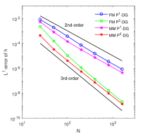
(a) $L^{1}$-error: $h$

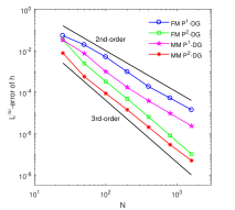
(b) $L^{\infty}$-error: $h$

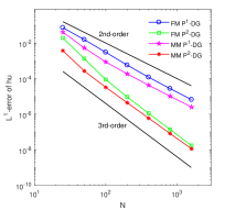
(c) $L^{1}$-error: $hu$

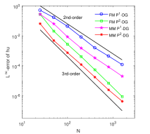
(d) $L^{\infty}$-error: $hu$

Figure 2: Example 4.1. The $L^{1}$ and $L^{\infty}$ norm of the error for the water depth $h=\eta-B$ and water discharge $hu$ is plotted as a function of $N$ for fixed and moving meshes.

Example 4.2

(The lake-at-rest steady-state flow test for the 1D SWEs over three different bottom topographies.)

We now test the well-balance property of the QLMM-DG method with two smooth topographies and a discontinuous topography,

$$B(x)=5e^{-\frac{2}{5}(x-5)^{2}},\quad x\in(0,10)$$ (4.5)

$$B(x)=\begin{cases}4,&\text{for }x\in(4,8)\\ 0,&\text{for }x\in(0,4)\cup(8,10)\end{cases}$$ (4.6)

$$B(x)=10e^{-\frac{2}{5}(x-5)^{2}},\quad x\in(0,10).$$ (4.7)

The initial solution is taken as the lake-at-rest steady state,

$$u=0,\quad\eta=h+B=10.$$

We expect that this steady-state solution is preserved since the QLMM-DG method is well-balanced. The final time is $T=0.5$.

The $L^{1}$ and $L^{\infty}$ error for $\eta$ and $hu$ is listed in Tables 1 and 2 for smooth $B$ (4.5) and in Tables 3 and 4 for discontinuous $B$ (4.6). We can observe that the error is at the level of round-off error (double precision in MATLAB), which demonstrates that the QLMM-DG method is well-balanced.

The bottom topography (4.7) (with a dry region) is used to demonstrate the well-balance and PP properties of the QLMM-DG method. This topography has a similar shape as (4.5) but its height touches the surface level at $x=5$ where $h=0$ initially. The computed water depth can have negative values during the computation and the application of the PP limiter is necessary. We computed the solution up to $t=0.5$. To ensure positivity preservation (cf. [31]), we take smaller CFL numbers as $0.3$ and $0.15$ for $P^{1}$-DG and $P^{2}$-DG, respectively, for this test. The $L^{1}$ and $L^{\infty}$ error for $h+B$ and $hu$ is listed in Tables 5 and 6 for $P^{1}$-DG and $P^{2}$-DG, respectively. The results clearly show that the QLMM-DG method is well-balanced.

Table 1: Example 4.2. Well-balance test for the $P^{1}$-DG method with fixed and moving meshes for smooth $B$ defined in (4.5).

	$\eta$		$hu$
$N$	$L^{1}$-error	$L^{\infty}$-error	$L^{1}$-error	$L^{\infty}$-error
	FM-DG method
25	4.288E-16	2.262E-15	8.582E-15	2.344E-14
50	4.143E-16	2.578E-15	1.541E-14	3.836E-14
100	1.431E-15	4.804E-15	2.537E-14	6.756E-14
	QLMM-DG method
25	6.726E-15	1.307E-14	1.196E-14	3.719E-14
50	1.185E-14	2.585E-14	2.153E-14	8.861E-14
100	2.303E-14	5.630E-14	3.731E-14	1.906E-13

Table 2: Example 4.2. Well-balance test for the $P^{2}$-DG method with fixed and moving meshes for smooth $B$ defined in (4.5)

	$\eta$		$hu$
$N$	$L^{1}$-error	$L^{\infty}$-error	$L^{1}$-error	$L^{\infty}$-error
	FM-DG method
25	4.697E-15	7.849E-15	1.771E-14	3.968E-14
50	4.813E-15	7.691E-15	1.617E-14	4.954E-14
100	4.919E-15	8.766E-15	3.464E-14	8.394E-14
	QLMM-DG method
25	1.510E-14	2.146E-14	1.510E-14	3.684E-14
50	2.289E-14	3.709E-14	3.102E-14	9.464E-14
100	4.132E-14	6.846E-14	4.847E-14	1.843E-13

Table 3: Example 4.2. Well-balance test for the $P^{1}$-DG method with fixed and moving meshes for discontinuous $B$ defined in (4.6).

	$\eta$		$hu$
$N$	$L^{1}$-error	$L^{\infty}$-error	$L^{1}$-error	$L^{\infty}$-error
	FM-DG method
25	3.540E-16	1.638E-15	5.512E-15	1.709E-14
50	3.530E-16	2.171E-15	1.310E-14	3.317E-14
100	3.499E-16	2.361E-15	2.185E-14	5.404E-14
	QLMM-DG method
25	5.445E-15	1.128E-14	1.113E-14	3.214E-14
50	1.316E-14	2.443E-14	1.926E-14	6.575E-14
100	2.344E-14	5.195E-14	4.425E-14	1.702E-13

Table 4: Example 4.2. Well-balance test for the $P^{2}$-DG method with fixed and moving meshes for discontinuous $B$ defined in (4.6).

	$\eta$		$hu$
$N$	$L^{1}$-error	$L^{\infty}$-error	$L^{1}$-error	$L^{\infty}$-error
	FM-DG method
25	4.517E-15	6.204E-15	1.088E-14	3.416E-14
50	4.682E-15	7.090E-15	1.876E-14	5.815E-14
100	4.482E-15	6.680E-15	1.967E-14	5.498E-14
	QLMM-DG method
25	1.393E-14	2.126E-14	1.840E-14	4.412E-14
50	2.177E-14	3.325E-14	3.417E-14	9.337E-14
100	4.194E-14	6.710E-14	4.863E-14	1.867E-13

Table 5: Example 4.2. Well-balance test for the $P^{1}$-DG method with fixed and moving meshes for the bottom topography (4.7) (with a dry region).

	$\eta$		$hu$
$N$	$L^{1}$-error	$L^{\infty}$-error	$L^{1}$-error	$L^{\infty}$-error
	$P^{1}$ FM-DG method
25	2.463E-16	1.142E-15	1.193E-14	2.986E-14
50	4.796E-16	2.175E-15	1.726E-14	4.508E-14
100	6.640E-16	2.897E-15	1.492E-14	5.099E-14
	$P^{1}$ QLMM-DG method
25	5.670E-15	1.136E-14	7.756E-15	3.501E-14
50	1.177E-14	2.691E-14	1.510E-14	7.347E-14
100	2.331E-14	5.537E-14	3.161E-14	1.801E-13

Table 6: Example 4.2. Well-balance test for the $P^{2}$-DG method with fixed and moving meshes for the bottom topography (4.7) (with a dry region).

	$\eta$		$hu$
$N$	$L^{1}$-error	$L^{\infty}$-error	$L^{1}$-error	$L^{\infty}$-error
	$P^{2}$ FM-DG method
25	4.513E-15	5.389E-15	2.117E-14	5.636E-14
50	4.579E-15	6.190E-15	3.079E-14	7.233E-14
100	4.644E-15	6.589E-15	3.433E-14	9.521E-14
	$P^{2}$ QLMM-DG method
25	1.460E-14	2.264E-14	1.847E-14	4.411E-14
50	2.686E-14	4.208E-14	4.812E-14	1.182E-13
100	4.887E-14	7.505E-14	5.989E-14	1.909E-13

Example 4.3

(The perturbed lake-at-rest steady-state flow test for the 1D SWEs.)

Following [8, 18, 19, 29, 30], we use this example to demonstrate that the QLMM-DG method is able to capture small perturbations of the lake-at-rest steady-state flow over non-flat bottom topography. We also use it to demonstrate the mesh adaptation ability of the method. The bottom topography in this example is taken as

$$B(x)=\begin{cases}0.25(\cos(10\pi(x-1.5))+1),&\text{for }x\in(1.4,1.6)\\ 0,&\text{for }x\in(0,1.4)\cup(1.6,2)\end{cases}$$ (4.8)

which has a bump in the middle of the physical interval. The initial conditions are

$$\eta(x,0)=\begin{cases}1+\varepsilon,&\text{for}~{}1.1\leq x\leq 1.2\\ 1,&\text{otherwise}\end{cases}\quad\hbox{and}\quad u(x,0)=0,$$

where $\varepsilon$ is a constant for the perturbation magnitude. We consider two cases, $\varepsilon=0.2$ (big pulse) and $\varepsilon=10^{-5}$ (small pulse). The initial conditions for both cases are plotted in Fig. 3. We use the transmissive boundary conditions and compute the solution up to $T=0.2$ when the right wave has passed the bottom bump.

The mesh trajectories obtained with the $P^{2}$-DG method and a moving mesh of $N=160$ are shown in Fig. 4. The obtained water surface level $\eta$ and discharge $hu$ are shown in Figs. 5 and 6 (for $\varepsilon=0.2$) and Figs. 7 and 8 (for $\varepsilon=10^{-5}$). It is interesting to observe that the initial wave splits into two waves at about $t=0.0165$ and the two waves propagate left and right at the characteristic speeds $\pm\sqrt{gh}$, respectively. The right-propagating wave interacts with the bottom bump and generates a complex wave structure in the bump region. Thus, it is beneficial to concentrate mesh points around the bump.

From the numerical results, we can see that the mesh points are concentrated around the waves before and after the split and in the region of the bottom bump. This is what we want as well as expect. To explain, we recall that the metric tensor for mesh adaptation is constructed based on the equilibrium variable $\mathcal{E}=u^{2}/2+g\eta$ and the water height $h$. It is not difficult to imagine that the mesh points concentrate around the waves because $\eta$ and thus $\mathcal{E}$ have significant changes there. Meanwhile, $\eta$ is constant in most places of the domain. Then, the spatial variations in $B$ are reflected in $h$, which in turn leads to the higher mesh concentration in the region of the bottom bump. Figs. 5, 6, 7, and 8 show that the QLMM-DG method is able to capture perturbations, small or large, of the lake-at-rest steady-state flow over non-flat bottom topography. Moreover, the moving mesh solutions with $N=160$ are more accurate than those with fixed meshes of $N=160$ and $N=480$ and contain no visible spurious numerical oscillations.

To verify the well-balance and positivity-preserving properties of the QLMM-DG method we increase the height of the bottom topography (4.9) to contain a dry region (near $x=1.5$),

$$\begin{split}&B(x)=\begin{cases}0.5(\cos(10\pi(x-1.5))+1),&\text{for }x\in(1.4,1.6)\\ 0,&\text{for }x\in(0,1.4)\cup(1.6,2).\end{cases}\end{split}$$ (4.9)

We repeat the computation with $\varepsilon=10^{-5}$. The bottom topography, the initial water level, and the mesh trajectories of $N=160$ obtained with the $P^{2}$ QLMM-DG method are plotted in Fig. 9. The mesh has higher concentration around the shock waves and the non-flat topography region. The mesh trajectories show that the right moving shock stops after it hits the dry region.

The water surface $\eta$ and discharge $hu$ obtained with $P^{2}$-DG and a moving mesh of $N=160$ and fixed meshes of $N=160$ and $N=640$ are plotted in Figs. 10 and 11. The results show that the DG method with moving or fixed meshes is able to capture the waves of small perturbation for situations containing dry regions. Moreover, the moving mesh solutions with $N=160$ are more accurate than those with fixed meshes of $N=160$ and $N=640$ and contain no visible spurious numerical oscillations.

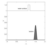
(a) Big pulse $\varepsilon=0.2$

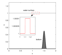
(b) Small pulse $\varepsilon=10^{-5}$

Figure 3: Example 4.3. The initial water surface level $\eta$ and the bottom topography $B$ are plotted for the pulse of $\varepsilon=0.2$ and $\varepsilon=10^{-5}$.

(a) Big pulse $\varepsilon=0.2$

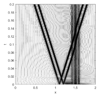
(b) Small pulse $\varepsilon=10^{-5}$

Figure 4: Example 4.3. The mesh trajectories are obtained with the $P^{2}$-DG method and a moving mesh of $N=160$ for the pulse of $\varepsilon=0.2$ and $\varepsilon=10^{-5}$.

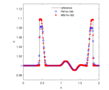
(a) $\eta$: FM 160 vs MM 160

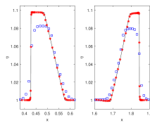
(b) Close view of (a)

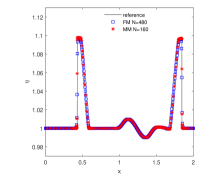
(c) $\eta$: FM 480 vs MM 160

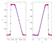
(d) Close view of (c)

Figure 5: Example 4.3. The water surface level $\eta$ at $t=0.2$ obtained with the $P^{2}$-DG method and a moving mesh of $N=160$ is compared with those obtained with fixed meshes of $N=160$ and $N=480$ for a large pulse $\varepsilon=0.2$.

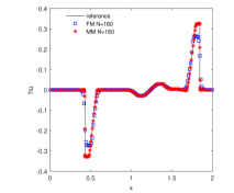
(a) $hu$: FM 160 vs MM 160

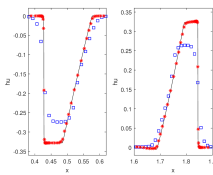
(b) Close view of (a)

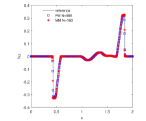
(c) $hu$: FM 480 vs MM 160

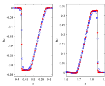
(d) Close view of (c)

Figure 6: Example 4.3. The water discharge $hu$ at $t=0.2$ obtained with the $P^{2}$-DG method and a moving mesh of $N=160$ is compared with those obtained with fixed meshes of $N=160$ and $N=480$ for a large pulse $\varepsilon=0.2$.

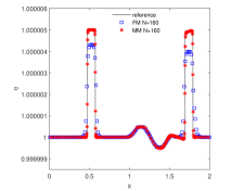
(a) $\eta$: FM 160 vs MM 160

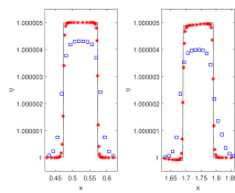
(b) Close view of (a)

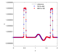
(c) $\eta$: FM 480 vs MM 160

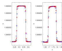
(d) Close view of (c)

Figure 7: Example 4.3. The water surface level $\eta$ at $t=0.2$ obtained with the $P^{2}$-DG method and a moving mesh of $N=160$ is compared with those obtained with fixed meshes of $N=160$ and $N=480$ for a small pulse $\varepsilon=10^{-5}$.

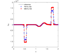
(a) $hu$: FM 160 vs MM 160

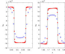
(b) Close view of (a)

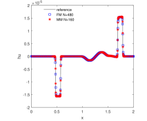
(c) $hu$: FM 480 vs MM 160

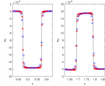
(d) Close view of (c)

Figure 8: Example 4.3. The water discharge $hu$ at $t=0.2$ obtained with the $P^{2}$-DG method and a moving mesh of $N=160$ is compared with those obtained with fixed meshes of $N=160$ and $N=480$ for a small pulse $\varepsilon=10^{-5}$.

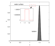
(a) Initial surface and bottom

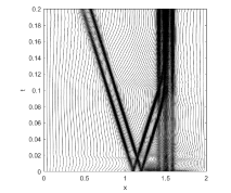
(b) Mesh trajectories

Figure 9: Example 4.3. (a) The initial water surface $\eta$ and the bottom $B$ (4.9) for the small perturbation test with a dry region. (b) The mesh trajectories obtained with $P^{2}$ QLMM-DG method of $N=160$.

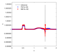
(a) $\eta$: FM 160 vs MM 160

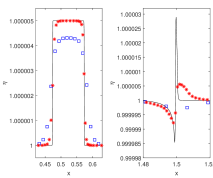
(b) Close view of (a)

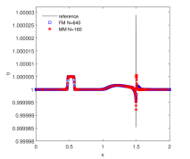
(c) $\eta$: FM 640 vs MM 160

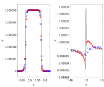
(d) Close view of (c)

Figure 10: Example 4.3 with the bottom topography (4.9) with a dry region. The water surface $\eta$ at $t=0.2$ obtained with $P^{2}$-DG and a moving mesh of $N=160$ are compared with those obtained with a fixed mesh of $N=160$ and $N=640$.

(a) $hu$: FM 160 vs MM 160

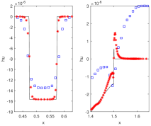
(b) Close view of (a)

(c) $hu$: FM 640 vs MM 160

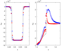
(d) Close view of (c)

Figure 11: Example 4.3 with the bottom topography (4.9) with a dry region. The water discharge $hu$ at $t=0.2$ obtained with $P^{2}$-DG and a moving mesh of $N=160$ are compared with those obtained with a fixed mesh of $N=160$ and $N=640$.

Example 4.4

(The rarefaction and shock waves test for the 1D SWEs with wavy bottom topography.)

In this example we compute the 1D SWEs with a wavy bottom topography [26]

$$B(x)=\begin{cases}0.3\cos^{30}(\frac{\pi}{2}(x-1)),&\text{for}~{}0\leq x\leq 2\\ 0,&\text{otherwise}.\end{cases}$$ (4.10)

The initial conditions are

$$\eta(x,0)=\begin{cases}2,&\text{for}~{}x\in(-10,1)\\ 0.35,&\text{for}~{}x\in(1,10)\\ \end{cases}\quad\quad u(x,0)=\begin{cases}1,&\text{for}~{}x\in(-10,1)\\ 0,&\text{for}~{}x\in(1,10).\\ \end{cases}$$

We choose the transmissive boundary conditions and compute the solution up to $T=1$. The solution contains several interesting features, including a rarefaction wave traveling left and two hydraulic jumps/shocks propagating right.

The mesh trajectories ($N=160$) are plotted in Fig. 12, showing that the mesh points concentrate properly around the rarefaction, the hydraulic jumps/shocks, and the region where $B$ is non-flat. Figs. 13 and 14 show the water surface level $\eta$ and water discharge $hu$ at $t=1$ obtained with $P^{2}$-DG and a moving mesh of $N=160$ and fixed meshes of $N=160$ and $N=1280$. It can be seen that the moving mesh solutions of $N=160$ are more accurate than those with a fixed mesh of $N=160$ and comparable with that with the fixed mesh of $N=1280$. Moreover, the QLMM-DG method does a good job in resolving the shock near $x=2$ which is known to be a difficult structure for a fixed-mesh method to resolve.

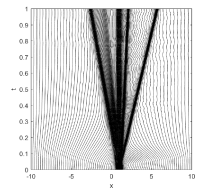
Figure 12: Example 4.4. The mesh trajectories are obtained with the $P^{2}$-DG method and a moving mesh of $N=160$.

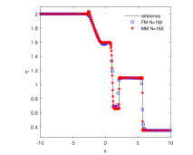
(a) $\eta$: FM 160 vs MM 160

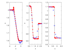
(b) Close view of (a)

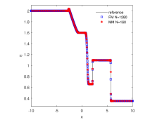
(c) $\eta$: FM 1280 vs MM 160

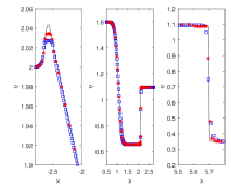
(d) Close view of (c)

Figure 13: Example 4.4. The water surface level $\eta$ at $t=1$ obtained with the $P^{2}$-DG method and a moving mesh of $N=160$ is compared with those obtained with fixed meshes of $N=160$ and $N=1280$.

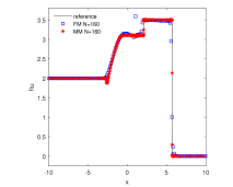
(a) $hu$: FM 160 vs MM 160

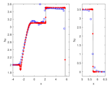
(b) Close view of (a)

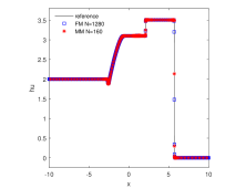
(c) $hu$: FM 1280 vs MM 160

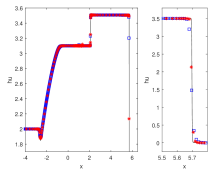
(d) Close view of (c)

Figure 14: Example 4.4. The water discharge $hu$ at $t=1$ obtained with the $P^{2}$-DG method and a moving mesh of $N=160$ is compared with those obtained with fixed meshes of $N=160$ and $N=1280$.

Example 4.5

(The lake-at-rest steady-state flow test for the 2D SWEs.)

We choose this example to verify the well-balance property of the QLMM-DG scheme in two dimensions. We solve the system on the domain $(x,y)\in(0,1)\times(0,1)$. The bottom topographies are the isolated elliptical-shaped bump [18] and read as

$$B(x,y)=0.8e^{-50\big{(}(x-0.5)^{2}+(y-0.5)^{2}\big{)}},$$ (4.11)

$$B(x,y)=e^{-50\big{(}(x-0.5)^{2}+(y-0.5)^{2}\big{)}}.$$ (4.12)

The initial water level and velocities are given by

$$\eta(x,y,0)=1,\quad u(x,y,0)=0,\quad v(x,y,0)=0.$$

The bottom topography (4.11) and (4.12) have the similar shape,and the latter contain a dry region near $(x,y)=(0.5,0.5)$. We use periodic boundary conditions for all unknown variables and compute the solution up to $t=0.1$. The flow surface should remain steady since the method is well-balanced.

An initial triangular mesh, shown in Fig. 15, is formed by dividing each cell of a rectangular mesh into four triangular elements. The $L^{1}$ and $L^{\infty}$ error for $\eta$, $hu$, and $hv$ are listed in Tables 7 and  8 for $P^{1}$-DG and $P^{2}$-DG, respectively, for the bottom topography (4.11). They show that our DG method, with either fixed or moving meshes, maintains the lake-at-rest steady state to the level of round-off error in both $L^{1}$ and $L^{\infty}$ norm.

To verify the well-balance and PP properties of the QLMM-DG method, we repeat the simulation for the bottom topography (4.12) where the application of the PP limiter to the water depth is necessary. The $L^{1}$ and $L^{\infty}$ error for $\eta$, $hu$, and $hv$ are listed in Tables 9 and  10 for $P^{1}$-DG and $P^{2}$-DG, respectively. One can see that the QLMM-DG method is well-balanced.

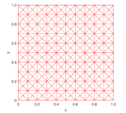
Figure 15: Example 4.5. An initial triangular mesh used in the computation is formed by dividing each cell of a rectangular mesh into 4 triangular elements.

Table 7: Example 4.5. Well-balance test for the $P^{1}$-DG method with fixed and moving meshes over bottom topography (4.11).

	$\eta$		$hu$		$hv$
$N$	$L^{1}$-error	$L^{\infty}$-error	$L^{1}$-error	$L^{\infty}$-error	$L^{1}$-error	$L^{\infty}$-error
	FM-DG method
$10\times 10\times 4$	1.539E-16	2.837E-16	1.257E-16	7.696E-16	1.343E-16	7.879E-16
$20\times 20\times 4$	1.957E-16	4.678E-16	1.690E-16	1.371E-15	1.829E-16	1.362E-15
$40\times 40\times 4$	3.259E-16	1.144E-15	2.614E-16	1.965E-15	2.750E-16	2.025E-15
	QLMM-DG method
$10\times 10\times 4$	1.109E-16	2.592E-16	1.335E-16	9.334E-16	1.337E-16	8.740E-16
$20\times 20\times 4$	1.149E-16	3.361E-16	1.660E-16	1.709E-15	1.671E-16	1.616E-15
$40\times 40\times 4$	1.146E-16	5.533E-16	2.567E-16	3.126E-15	2.580E-16	3.087E-15

Table 8: Example 4.5. Well-balance test for the $P^{2}$-DG method with fixed and moving meshes over bottom topography (4.11).

	$\eta$		$hu$		$hv$
$N$	$L^{1}$-error	$L^{\infty}$-error	$L^{1}$-error	$L^{\infty}$-error	$L^{1}$-error	$L^{\infty}$-error
	FM-DG method
$10\times 10\times 4$	4.287E-16	1.841E-15	8.615E-16	4.685E-15	9.310E-16	5.907E-15
$20\times 20\times 4$	4.020E-16	3.239E-15	8.930E-16	5.358E-15	9.638E-16	7.076E-15
$40\times 40\times 4$	4.454E-16	4.503E-15	1.056E-15	9.702E-15	1.129E-15	1.281E-14
	QLMM-DG method
$10\times 10\times 4$	4.795E-16	1.841E-15	7.965E-16	4.949E-15	8.029E-16	4.821E-15
$20\times 20\times 4$	5.023E-16	2.642E-15	9.442E-16	5.800E-15	8.870E-16	5.128E-15
$40\times 40\times 4$	5.155E-16	3.598E-15	1.428E-15	1.063E-14	1.167E-15	7.697E-15

Table 9: Example 4.5. Well-balance test for the $P^{1}$-DG method with fixed and moving meshes over bottom topography (4.12) (with a dry region).

	$\eta$		$hu$		$hv$
$N$	$L^{1}$-error	$L^{\infty}$-error	$L^{1}$-error	$L^{\infty}$-error	$L^{1}$-error	$L^{\infty}$-error
	FM-DG method
$10\times 10\times 4$	1.256E-16	5.706E-16	1.674E-16	1.631E-15	1.639E-16	1.924E-15
$20\times 20\times 4$	1.314E-16	1.368E-15	1.777E-16	2.543E-15	1.926E-16	2.684E-15
$40\times 40\times 4$	1.434E-16	4.448E-15	2.224E-16	3.081E-15	2.455E-16	4.990E-15
	QLMM-DG method
$10\times 10\times 4$	1.026E-16	5.661E-16	1.497E-16	1.349E-15	1.524E-16	1.511E-15
$20\times 20\times 4$	9.847E-17	1.555E-15	1.930E-16	2.047E-15	1.987E-16	2.055E-15
$40\times 40\times 4$	8.793E-17	6.290E-15	2.351E-16	3.217E-15	2.356E-16	3.168E-15

Table 10: Example 4.5. Well-balance test for the $P^{2}$-DG method with fixed and moving meshes over bottom topography (4.12) (with a dry region).

	$\eta$		$hu$		$hv$
$N$	$L^{1}$-error	$L^{\infty}$-error	$L^{1}$-error	$L^{\infty}$-error	$L^{1}$-error	$L^{\infty}$-error
	FM-DG method
$10\times 10\times 4$	4.830E-16	1.673E-14	9.355E-16	1.432E-14	9.978E-16	1.315E-14
$20\times 20\times 4$	5.039E-16	6.368E-14	9.708E-16	2.008E-14	1.053E-15	2.865E-14
$40\times 40\times 4$	5.421E-16	1.280E-13	1.199E-15	2.173E-14	1.274E-15	2.015E-14
	QLMM-DG method
$10\times 10\times 4$	5.735E-16	1.623E-14	8.498E-16	1.366E-14	8.691E-16	1.461E-14
$20\times 20\times 4$	6.264E-16	5.730E-14	9.876E-16	1.663E-14	9.285E-16	2.035E-14
$40\times 40\times 4$	7.067E-16	1.021E-13	1.411E-15	1.231E-14	1.163E-15	1.243E-14

Example 4.6

(The perturbed lake-at-rest steady-state flow test for the 2D SWEs.)

We choose this example first used by LeVeque [18] to demonstrate the ability of the QLMM-DG method to simulate small perturbations of the water surface. The bottom topography is an isolated elliptical shaped hump,

$$B(x,y)=0.8e^{\big{(}-5(x-0.9)^{2}-50(y-0.5)^{2}\big{)}},\quad(x,y)\in(-1,2)\times(0,1).$$ (4.13)

The initial conditions are given by

$$\begin{split}&\eta(x,y,0)=\begin{cases}1+0.01,&\hbox{for~{}$x\in(0.05,0.15)$}\\ 1,&\hbox{otherwise}\\ \end{cases}\\ &u(x,y,0)=0,\quad\hbox{and}\quad v(x,y,0)=0.\end{split}$$

Reflection boundary conditions [27] are used for all domain boundary. Theoretically, this perturbation splits into two waves, propagating left and right at the characteristic speeds $\pm\sqrt{gh}$. One of these waves is moving towards the bump in the bottom topography, interacting with it, and generating a complex wave structure. The difficulty of this test case is to resolve the waves that are very small in magnitude in comparison to the average values of the quantities.

The moving mesh of $N=150\times 50\times 4$ at $t=0.12,0.24,0.36,0.48$ obtained with $P^{2}$ QLMM-DG method are shown in Fig. 16. The contours of the obtained solutions $\eta$, $hu$, and $hv$ are shown in Figs. 17 – 20. For comparison purpose, the numerical solutions obtained with fixed meshes of $N=150\times 50\times 4$ and $N=600\times 200\times 4$ are also shown. We can see that the mesh points concentrate correctly around the waves and the point $(x,y)=(0.9,0.5)$, the center of the non-flat region of the bottom topography. Moreover, the QLMM-DG method resolves well the complex small-scale features of the water flow. The moving mesh solutions with $N=150\times 50\times 4$ do not contain visibly spurious oscillations and is more accurate than that with a fixed mesh of $N=150\times 50\times 4$ and comparable with that with a fixed mesh of $N=600\times 200\times 4$.

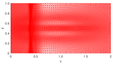
(a) Mesh at $t=0.12$

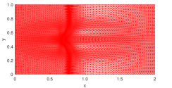
(b) Mesh at $t=0.24$

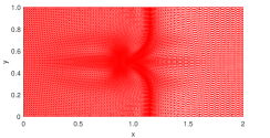
(c) Mesh at $t=0.36$

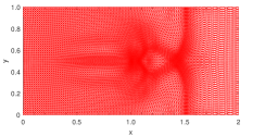
(d) Mesh at $t=0.48$

Figure 16: Example 4.6. The moving mesh of $N=150\times 50\times 4$ at $t=0.12,~{}0.24,~{}0.36,~{}0.48$ is obtained with the $P^{2}$ QLMM-DG method.

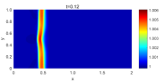
(a) $\eta$: MM $N=150\times 50\times 4$

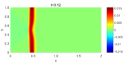
(b) $hu$: MM $N=150\times 50\times 4$

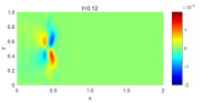
(c) $hv$: MM $N=150\times 50\times 4$

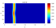
(d) $\eta$: FM $N=150\times 50\times 4$

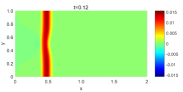
(e) $hu$: FM $N=150\times 50\times 4$

(f) $hv$: FM $N=150\times 50\times 4$

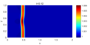
(g) $\eta$: FM $600\times 200\times 4$

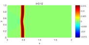
(h) $hu$: FM $N=600\times 200\times 4$

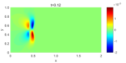
(i) $hv$: FM $N=600\times 200\times 4$

Figure 17: Example 4.6. The contours at $t=0.12$ of $\eta$, $hu$, and $hv$ at $t=0.12$ are obtained with the $P^{2}$ QLMM-DG method and a moving mesh of $N=150\times 50\times 4$ and fixed meshes of $N=150\times 50\times 4$ and $N=600\times 200\times 4$.

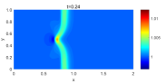
(a) $\eta$: MM $N=150\times 50\times 4$

(b) $hu$: MM $N=150\times 50\times 4$

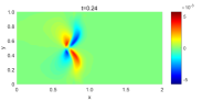
(c) $hv$: MM $N=150\times 50\times 4$

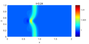
(d) $\eta$: FM $N=150\times 50\times 4$

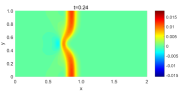
(e) $hu$: FM $N=150\times 50\times 4$

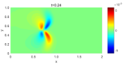
(f) $hv$: FM $N=150\times 50\times 4$

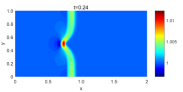
(g) $\eta$: FM $600\times 200\times 4$

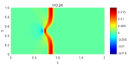
(h) $hu$: FM $N=600\times 200\times 4$

(i) $hv$: FM $N=600\times 200\times 4$

Figure 18: Continuation of Fig. 17: $t=0.24$.

(a) $\eta$: MM $N=150\times 50\times 4$

(b) $hu$: MM $N=150\times 50\times 4$

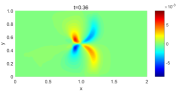
(c) $hv$: MM $N=150\times 50\times 4$

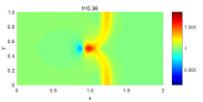
(d) $\eta$: FM $N=150\times 50\times 4$

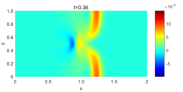
(e) $hu$: FM $N=150\times 50\times 4$

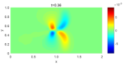
(f) $hv$: FM $N=150\times 50\times 4$

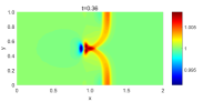
(g) $\eta$: FM $600\times 200\times 4$

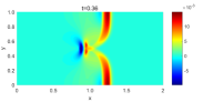
(h) $hu$: FM $N=600\times 200\times 4$

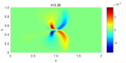
(i) $hv$: FM $N=600\times 200\times 4$

Figure 19: Continuation of Fig. 17: $t=0.36$.

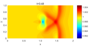
(a) $\eta$: MM $N=150\times 50\times 4$

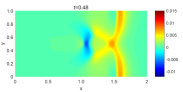
(b) $hu$: MM $N=150\times 50\times 4$

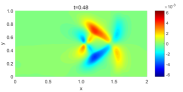
(c) $hv$: MM $N=150\times 50\times 4$

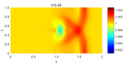
(d) $\eta$: FM $N=150\times 50\times 4$

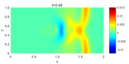
(e) $hu$: FM $N=150\times 50\times 4$

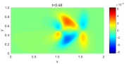
(f) $hv$: FM $N=150\times 50\times 4$

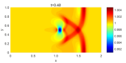
(g) $\eta$: FM $600\times 200\times 4$

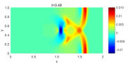
(h) $hu$: FM $N=600\times 200\times 4$

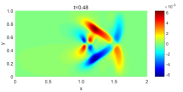
(i) $hv$: FM $N=600\times 200\times 4$

Figure 20: Continuation of Fig. 17: $t=0.48$.

5 Conclusions

We have developed a high-order, well-balanced, positivity-preserving quasi-Lagrange moving mesh DG (QLMM-DG) method for the SWEs with non-flat bottom topography in the previous sections. The method combines the quasi-Lagrange moving mesh DG method [21, 33] with the hydrostatic reconstruction technique [1, 30, 32] and a change of unknown variables to achieve the well-balance property. Specifically, we use the new variables $(\eta=h+B,\,hu,\,hv)$ instead of the original ones $(h,\,hu,\,hv)$ and rewrite the flux in a special form (2.2) where some $h$ are replaced by $\eta$ and the others remain the same. In the construction of the DG numerical flux, the value of $h$ is modified using the hydrostatic reconstruction technique whereas $\eta$ stays unmodified. It has been shown that the method, in both semi-discrete and fully discrete forms, preserves the lake-at-rest steady-state solutions while maintaining the high-order accuracy of DG methods. It has also been shown that a QLMM-DG scheme can be developed based on the SWEs in the original variables $(h,\,hu,\,hv)$ but it is well-balanced only in semi-discrete form.

It is worth pointing out that the bottom topography $B$ needs to be updated on the new mesh at each time step. In the rezoning moving mesh DG method recently developed in [35], it is required that $B$ be updated using the same scheme as that for the flow variables to attain the well-balance property. This makes the choice of the scheme for updating $B$ limited. A DG-interpolation scheme [34] has been used in [35] for the purpose. In contrast, there is no constraint on the choice of the scheme for updating $B$ in the current QLMM-DG method. We have used $L^{2}$-projection for updating $B$ in our computation since it is straightforward and economic to implement.

It should be emphasized that the water depth should be kept nonnegative in the computation. Following [31, 32], we use a linear scaling positivity-preserving limiter [22, 39, 40] to ensure the nonnegativity of the water depth. To recover the well-balance property violated by the PP limiter, a high-order correction is made to the approximation of the bottom topography according to the modifications in the water depth due to the PP limiting; see (2.29).

The numerical results for a selection of one- and two-dimensional examples have been presented to demonstrate the well-balance and positive-preserving properties and high-order accuracy of the QLMM-DG method. They have also shown that the method works well for the lake-at-rest steady state and its perturbations and is able to adapt the mesh according to structures in the flow and bottom topography.

Appendix A The MMPDE moving mesh method

In this appendix we describe the generation of the new physical mesh $\mathcal{T}^{n+1}_{h}$ from the old one $\mathcal{T}^{n}_{h}$ using the MMPDE moving mesh method [11, 12, 13]. We use the $\bm{\xi}$-formulation of the method and its new implementation proposed in [14].

For mesh generation purpose, we introduce a computational mesh $\mathcal{T}_{c}$ with the vertices $\bm{\xi}_{1},\;...,\;\bm{\xi}_{N_{v}}$ and a physical mesh $\mathcal{T}_{h}$ with the vertices $\bm{x}_{1},\;...,\;\bm{x}_{N_{v}}$ which can be viewed as deformations of the mesh $\mathcal{T}^{n}_{h}$. These two meshes serve as intermediate variables. We also assume that a reference computational mesh $\hat{\mathcal{T}}_{c}=\{\hat{\bm{\xi}}_{1},\;...,\;\hat{\bm{\xi}}_{N_{v}}\}$ has been given. This mesh is kept fixed in the computation and should be chosen as uniform as possible. Often it can be taken as the initial physical mesh.

A key idea of the MMPDE method is to view any nonuniform mesh as a uniform one in some Riemannian metric [13]. The metric tensor $\mathbb{M}$, a symmetric and uniformly positive definite matrix-valued function defined on $\mathcal{D}$, provides the information needed for determining the size, shape, and orientation of the mesh elements throughout the domain. A choice of $\mathbb{M}$ has been given in §4.

Since $\mathcal{T}_{h}$ and $\mathcal{T}_{c}$ can be viewed as deformations of $\mathcal{T}^{n}_{h}$, for any element $K\in\mathcal{T}_{h}$, there exits an element $K_{c}\in\mathcal{T}_{c}$ corresponding to $K$. Denote the affine mapping from $K_{c}$ to $K$ as $F_{K}$ and its Jacobian matrix as $F^{\prime}_{K}$. It is known [13] that any mesh $\mathcal{T}_{h}$ which is uniform in the metric $\mathbb{M}$ in reference to $\mathcal{T}_{c}$, satisfies

$$|K|\sqrt{\det(\mathbb{M}_{K})}=\frac{\sigma_{h}|K_{c}|}{|\mathcal{D}_{c}|}, \quad\forall K\in\mathcal{T}_{h}$$ (A.1)

$$\frac{1}{d}\hbox{tr}\big{(}(F^{\prime}_{K})^{-1}\mathbb{M}_{K}^{-1}(F^{\prime}_{K})^{-T}\big{)}=\hbox{det}\big{(}(F^{\prime}_{K})^{-1}\mathbb{M}_{K}^{-1}(F^{\prime}_{K})^{-T}\big{)}^{\frac{1}{d}}, \quad\forall K\in\mathcal{T}_{h}$$ (A.2)

where $d$ is the dimension of the domain ($d=2$ in two dimensions), $\hbox{tr}(\cdot)$ and $\hbox{det}(\cdot)$ denote the trace and determinant of a matrix, respectively, $\mathbb{M}_{K}$ is the average of $\mathbb{M}$ over $K$, and

$$|\mathcal{D}_{c}|=\sum\limits_{K_{c}\in\mathcal{T}_{c}}|K_{c}|,\quad\sigma_{h}=\sum\limits_{K\in\mathcal{T}_{h}}|K|\hbox{det}(\mathbb{M}_{K})^{\frac{1}{2}}.$$

Condition (A.1) is called the equidistribution condition that determines the size of elements through the metric tensor $\mathbb{M}$ and requires that all the elements have the same size in the metric tensor $\mathbb{M}$. Condition (A.2) is called the alignment condition that determines the shape and orientation of $K$ through $\mathbb{M}$ and the shape of $K_{c}$ and requires that $K$, when measured in the metric $\mathbb{M}_{K}$, be similar to $K_{c}$ measured in the Euclidean metric. A mesh energy function, with its minimization resulting in a mesh satisfying the equidistribution and alignment conditions as closely as possible, is given by

$$\begin{split}I_{h}(\mathcal{T}_{h};\mathcal{T}_{c})=&\frac{1}{3}\sum_{K\in\mathcal{T}_{h}}|K|\hbox{det}(\mathbb{M}_{K})^{\frac{1}{2}}\big{(}\hbox{tr}((F^{\prime}_{K})^{-1}\mathbb{M}^{-1}_{K}(F^{\prime}_{K})^{-T})\big{)}^{\frac{3d}{4}}\\ &+\frac{1}{3}d^{\frac{3d}{4}}\sum_{K\in\mathcal{T}_{h}}|K|\hbox{det}(\mathbb{M}_{K})^{\frac{1}{2}}\left(\hbox{det}(F^{\prime}_{K})\hbox{det}(\mathbb{M}_{K})^{\frac{1}{2}}\right)^{-\frac{3}{2}},\end{split}$$ (A.3)

which is a Riemann sum of a continuous functional developed in [13].

For a given mesh $\mathcal{T}_{h}^{n}$, we want to find a new mesh $\mathcal{T}_{h}^{n+1}$ by minmimizing $I_{h}$. Notice that $I_{h}(\mathcal{T}_{h},\mathcal{T}_{c})$ is a function of $\mathcal{T}_{c}$ and $\mathcal{T}_{h}$ or a function of their vertices. We take $\mathcal{T}_{h}$ as $\mathcal{T}_{h}^{n}$, minimize $I_{h}(\mathcal{T}_{h}^{n},\mathcal{T}_{c})$ with respect to $\mathcal{T}_{c}$ (and denote the final mesh as $\mathcal{T}_{c}^{n+1}$), and obtain $\mathcal{T}_{h}^{n+1}$ through the relation between $\mathcal{T}_{h}^{n}$ and $\mathcal{T}_{c}^{n+1}$. The minimization of $I_{h}(\mathcal{T}_{h}^{n},\mathcal{T}_{c})$ is carried out by solving the mesh equation defined as the gradient system of the energy function (the MMPDE approach), i.e.,

$$\begin{split}\frac{d\bm{\xi}_{i}}{dt}=-\frac{\hbox{det}(\mathbb{M}(\bm{x_{i}}))^{\frac{1}{2}}}{\tau}\Big{(}\frac{\partial I_{h}}{\partial\boldsymbol{\xi}_{i}}\Big{)}^{T},\quad i=1,...,N_{v}\end{split}$$ (A.4)

where ${\partial I_{h}}/{\partial\bm{\xi}_{i}}$ is considered as a row vector and $\tau>0$ is a parameter used to adjust the response time of mesh movement to the changes in $\mathbb{M}$. We take $\tau=0.1N^{-\frac{1}{d}}$ in our computation. Define a function $G$ associated with the energy (A.3) as

$$G(\mathbb{J},\hbox{det}(\mathbb{J}))=\frac{1}{3}\hbox{det}(\mathbb{M}_{K})^{\frac{1}{2}}(\hbox{tr}(\mathbb{J}\mathbb{M}_{K}^{-1}\mathbb{J}^{T}))^{\frac{3d}{4}}+\frac{1}{3}d^{\frac{3d}{4}}\hbox{det}(\mathbb{M}_{K})^{\frac{1}{2}}\left(\frac{\hbox{det}(\mathbb{J})}{\hbox{det}(\mathbb{M}_{K})^{\frac{1}{2}}}\right)^{\frac{3}{2}},$$ (A.5)

where $\mathbb{J}=(F^{\prime}_{K})^{-1}=E_{K_{c}}E_{K}^{-1}$ and $E_{K}=[\bm{x}_{1}^{K}-\bm{x}_{0}^{K},\;...,\;\bm{x}_{d}^{K}-\bm{x}_{0}^{K}]$ and $E_{K_{c}}=[\bm{\xi}_{1}^{K}-\bm{\xi}_{0}^{K},\;...,\;\bm{\xi}_{d}^{K}-\bm{\xi}_{0}^{K}]$ are the edge matrices of $K$ and $K_{c}$, respectively. By scalar-by-matrix differentiation, we can obtain the derivatives of $G$ with respect to $\mathbb{J}$ and $\hbox{det}(\mathbb{J})$ [14] as

$$\frac{\partial G}{\partial\mathbb{J}}=\frac{d}{2}\hbox{det}(\mathbb{M}_{K})^{\frac{1}{2}}(\hbox{tr}(\mathbb{J}\mathbb{M}_{K}^{-1}\mathbb{J}^{T}))^{\frac{3d}{4}-1}\mathbb{M}_{K}^{-1}\mathbb{J}^{T},$$ (A.6)

$$\frac{\partial G}{\partial\hbox{det}(\mathbb{J})}=\frac{1}{2}d^{\frac{3d}{4}}\hbox{det}(\mathbb{M}_{K})^{-\frac{1}{4}}\hbox{det}(\mathbb{J})^{\frac{1}{2}}.$$ (A.7)

Using these formulas, we can rewrite (A.4) as

$$\begin{split}\frac{d\bm{\xi}_{i}}{dt}=\frac{\hbox{det}(\mathbb{M}(\bm{x_{i}}))^{\frac{1}{2}}}{\tau}\sum_{K\in\omega_{i}}|K|\bm{v}^{K}_{i_{K}},\quad i=1,...,N_{v}\end{split}$$ (A.8)

where $\omega_{i}$ is the element patch associated with the vertex $\bm{x}_{i}$, $i_{K}$ is the local index of $\bm{x}_{i}$ on $K$, and $\bm{v}^{K}_{i_{K}}$ is the local velocity contributed by the element $K$ to the vertex $i_{K}$. The local velocities associated with $K$ are given by

$$\begin{split}\left[\begin{array}[]{c}(\bm{v}_{1}^{K})^{T}\\ (\bm{v}_{2}^{K})^{T}\\ \vdots\\ (\bm{v}_{d}^{K})^{T}\\ \end{array}\right]=-E_{K}^{-1}\frac{\partial G}{\partial\mathbb{J}}-\frac{\partial G}{\partial\hbox{det}(\mathbb{J})}\frac{\hbox{det}(E_{K_{c}})}{\hbox{det}(E_{K})}E_{K_{c}}^{-1},\quad\bm{v}^{K}_{0}=-\sum_{i=1}^{d}\bm{v}^{K}_{i}.\end{split}$$ (A.9)

We emphasize that the velocities for the boundary nodes must be modified properly. For example, they should be set to be zero for the corner vertices. For other boundary vertices, the velocities should be modified such that their normal components along the domain boundary are zeros so they slide only along the boundary and do not move out of the domain.

Starting with the reference computational mesh $\hat{\mathcal{T}}_{c}$ as the initial mesh, the mesh equation (A.8) is integrated over a physical time step. The obtained new mesh is denoted by $\mathcal{T}_{c}^{n+1}$. Notice that $\mathcal{T}_{h}^{n}$ is kept fixed during the integration and forms a correspondence with $\mathcal{T}_{c}^{n+1}$. We denote this correspondence formally by $\mathcal{T}_{h}^{n}=\Phi_{h}(\mathcal{T}_{c}^{n+1})$ with $\bm{x}_{i}^{n}=\Phi_{h}(\bm{\xi}_{i}^{n+1})$, $i=1,...,N_{v}$. Then the new physical mesh $\mathcal{T}_{h}^{n+1}$ is defined as $\mathcal{T}_{h}^{n+1}=\Phi_{h}(\hat{\mathcal{T}}_{c})$ with $\bm{x}_{i}^{n+1}=\Phi_{h}(\hat{\bm{\xi}}_{i})$, $i=1,...,N_{v}$. Notice that $\mathcal{T}_{h}^{n+1}$ can be computed using linear interpolation.

References

[1]
E. Audusse, F. Bouchut, M.-O. Bristeau, R. Klein, and B. Perthame,
A fast and stable well-balanced scheme with hydrostatic reconstruction for shallow water flows,
SIAM J. Sci. Comput., 25 (2004), 2050-2065.
[2]
L. Arpaia and M. Ricchiuto,
r-adaptation for shallow water flows: conservation, well balancedness, efficiency,
Comput. & Fluids, 160 (2018), 175-203.
[3]
A. Bermudez and M. E. Vazquez,
Upwind methods for hyperbolic conservation laws with source terms,
Comput. & Fluids, 23 (1994), 1049-1071.
[4]
B. Cockburn and C.-W. Shu,
TVB Runge-Kutta local projection discontinuous Galerkin finite element method for conservation laws II: General framework,
Math. Comp., 52 (1989), 411-435.
[5] B. Cockburn, S.-Y. Lin, and C.-W. Shu,
TVB Runge-Kutta local projection discontinuous Galerkin finite element method for
conservation laws III: one dimensional systems,
J. Comput. Phys., 84 (1989), 90-113.
[6]
B. Cockburn and C.-W. Shu,
The Runge-Kutta discontinuous Galerkin method for conservation laws V: multidimensional systems,
J. Comput. Phys., 141 (1998), 199-224.
[7]
B. Cockburn and C.-W. Shu,
Runge-Kutta discontinuous Galerkin methods for convection dominated problems,
J. Sci. Comput., 16 (2001), 173-261.
[8]
R. Donat, M. C. Martí, A. Martínez-Gavara, and P. Mulet,
Well-balanced adaptive mesh refinement for shallow water flows,
J. Comput. Phys., 257 (2014), 937-953.
[9]
C. Eskilsson and S. J. Sherwin,
A triangular spectral/ discontinuous Galerkin method for modelling 2D shallow water equations,
Int. J. Numer. Meth. Fluids, 45 (2004), 605-623.
[10]
A. Ern, S. Piperno, and K. Djadel,
A well-balanced Runge-Kutta discontinuous Galerkin method for the shallow-water equations with flooding and drying,
Int. J. Numer. Meth. Fluids, 58 (2008), 1-25.
[11]
W. Huang, Y. Ren, and R. Russell,
Moving mesh partial differential equations (MMPDEs) based upon the equidistribution principle,
SIAM J. Numer. Anal., 31 (1994), 709-730.
[12]
W. Huang and W. Sun,
Variational mesh adaptation II: error estimates and monitor functions,
J. Comput. Phys., 184 (2003), 619-648.
[13]
W. Huang and R. Russell,
Adaptive Moving Mesh Methods,
Springer, New York, Applied Mathematical Sciences Series, Vol. 174 (2011).
[14]
W. Huang and L. Kamenski,
A geometric discretization and a simple implementation for variational mesh generation and adaptation,
J. Comput. Phys., 301 (2015), 322-337.
[15]
W. Huang and L. Kamenski,
On the mesh nonsingularity of the moving mesh PDE method,
Math. Comp., 87 (2018), 1887-1911.
[16]
A. Kurganov and D. Levy,
Central-upwind schemes for the Saint-Venant system,
ESAIM: M2AN , 36 (2002), 397-425.
[17]
P. Lamby, S. Müller, and Y. Stiriba,
Solution of shallow water equations using fully adaptive multiscale schemes,
Int. J. Numer. Meth. Fluids, 49 (2005), 417–437.
[18]
R. LeVeque,
Balancing source terms and flux gradients in high-resolution godunov methods: the quasi-steady wave-propagation algorithm,
J. Comput. Phys., 146 (1998), 346-365.
[19]
G. Li, L. Song, and J. Gao,
High order well-balanced discontinuous Galerkin methods based on hydrostatic reconstruction for shallow water equations,
J. Comput. App. Math., 340 (2018), 546-560.
[20]
C. Lu, J. Qiu, and R. Wang,
A numerical study for the performance of the WENO schemes based on different numerical fluxes for the shallow water equations,
J. Comp. Math., 28 (2010), 807-825.
[21]
D. Luo, W. Huang, and J. Qiu,
A quasi-Lagrange moving mesh discontinuous Galerkin method for hyperbolic conservation laws,
J. Comput. Phys., 396 (2019), 544-578.
[22]
X.-D. Liu and S. Osher,
Non-oscillatory high order accurate self similar maximum principle satisfying shock capturing schemes,
SIAM J. Numer. Anal., 33 (1996), 760-779.
[23]
J.-F. Remacle, S. S. Frazao, X. Li, and M. Shephard,
Adaptive discontinuous Galerkin method for the shallow water equations,
Int. J. Numer. Meth. Fluids, 52 (2006), 903-923.
[24]
P. D. Thomas and C. K. Lombard,
Geometric conservation law and its application to flow computations on moving grids,
AIAA J., 17 (1979), 1030-1037.
[25]
J. G. Trulio and K. R. Trigger,
Numerical solution of the one-dimensional hydrodydnamic equations in an arbitrary time-dependent coordinate system, Report UCLR-6522,
Lawrence Radiation Laboratory, University of California, Berkeley, 1961.
[26]
H. Tang,
Solution of the shallow-water equations using an adaptive moving mesh method,
Int. J. Numer. Meth. Fluids, 44 (2004), 789-810.
[27]
G. Tumolo, L. Bonaventura, and M. Restelli,
A semi-implicit, semi-lagrangian, -adaptive discontinuous Galerkin method for the shallow water equations,
J. Comput. Phys., 232 (2013), 46-67.
[28]
Y. Xing and C.-W. Shu,
High order finite difference WENO schemes with the exact conservation property for the shallow water equations,
J. Comput. Phys., 208 (2005), 206-227.
[29]
Y. Xing and C.-W. Shu,
High order well-balanced finite volume WENO schemes and discontinuous Galerkin methods for a class of hyperbolic systems with source terms,
J. Comput. Phys., 214 (2006), 567-598.
[30]
Y. Xing and C.-W. Shu,
A new approach of high order well-balanced finite volume WENO schemes and discontinuous Galerkin methods for a class of hyperbolic systems with
source terms,
Commun. Comput. Phys., 1 (2006), 100-134.
[31]
Y. Xing, X. Zhang, and C.-W. Shu,
Positivity-preserving high order well-balanced discontinuous Galerkin methods
for the shallow water equations,
Adv. Water Resourc., 33 (2010), 1476-1493.
[32]
Y. Xing and X. Zhang,
Positivity-preserving well-balanced discontinuous Galerkin methods for the shallow water equations on unstructured triangular meshes,
J. Sci. Comput., 57 (2013), 19-41.
[33]
M. Zhang, J. Cheng, W. Huang, and J. Qiu,
An adaptive moving mesh discontinuous Galerkin method for the radiative transfer equation,
Commun. Comput. Phys., 27 (2020), 1140-1173.
[34]
M. Zhang, W. Huang, and J. Qiu,
High-order conservative positivity-preserving DG-interpolation for deforming meshes and application to moving mesh DG simulation of radiative transfer,
SIAM J. Sci. Comput., to appear. arXiv:1910.11931.
[35]
M. Zhang, W. Huang, and J. Qiu,
A high-order well-balanced positivity-preserving moving mesh DG method for the shallow water equations with non-flat bottom topography,
arXiv:2006.15187.
[36]
Z. Zhang and A. Naga,
A new finite element gradient recovery method: Superconvergence property,
SIAM J. Sci. Comput., 26 (2005), 1192-1213.
[37]
F. Zhou, G. Chen, S. Noelle, and H. Guo,
A well-balanced stable generalized Riemann problem scheme for shallow water equations using adaptive moving unstructured triangular meshes.
Int. J. Numer. Meth. Fluids, 73 (2013), 266-283.
[38]
J. G. Zhou, D. M. Causon, C. G. Mingham, and D. M. Ingram,
The surface gradient method for the treatment of source terms in the shallow-water equations,
J. Comput. Phys., 168 (2001), 1-25.
[39]
X. Zhang and C.-W. Shu,
On positivity preserving high order discontinuous Galerkin methods for compressible Euler equations
on rectangular meshes,
J. Comput. Phys., 229 (2010), 8918-8934.
[40]
X. Zhang, Y. Xia, and C.-W. Shu,
Maximum-principle-satisfying and positivity-preserving high order discontinuous Galerkin schemes
for conservation laws on triangular meshes,
J. Sci. Comput., 50 (2012), 29-62.