Robust Reinforcement Learning: A Case Study in Linear Quadratic Regulation

Abstract

This paper studies the robustness of reinforcement learning algorithms to errors in the learning process. Specifically, we revisit the benchmark problem of discrete-time linear quadratic regulation (LQR) and study the long-standing open question: Under what conditions is the policy iteration method robustly stable from a dynamical systems perspective? Using advanced stability results in control theory, it is shown that policy iteration for LQR is inherently robust to small errors in the learning process and enjoys small-disturbance input-to-state stability: whenever the error in each iteration is bounded and small, the solutions of the policy iteration algorithm are also bounded, and, moreover, enter and stay in a small neighbourhood of the optimal LQR solution. As an application, a novel off-policy optimistic least-squares policy iteration for the LQR problem is proposed, when the system dynamics are subjected to additive stochastic disturbances. The proposed new results in robust reinforcement learning are validated by a numerical example.

Introduction

As an important and popular method in reinforcement learning (RL), policy iteration has been widely studied by researchers and utilized in different kinds of real-life applications by practitioners (Bertsekas 1995; Sutton and Barto 2018). Policy iteration involves two steps, policy evaluation and policy improvement. In policy evaluation, a given policy is evaluated based on a scalar performance index. Then this performance index is utilized to generate a new control policy in policy improvement. These two steps are iterated in turn, to find the solution of the RL problem at hand. When all the information involved in this process is exactly known, the convergence to the optimal solution can be provably guaranteed, by exploiting the monotonicity property of the policy improvement step. That is, the performance of the newly generated policy is no worse than that of the given policy in each iteration. Over the past decades, various versions of policy iteration have been proposed, for diverse optimal control problems, see (Bertsekas 1995; Sutton and Barto 2018; Lewis, Vrabie, and Syrmos 2012; Jiang and Jiang 2017; Jiang, Bian, and Gao 2020) and the references therein.

In reality, policy evaluation or policy improvement can hardly be implemented precisely, because of the existence of various errors, which may be induced by function approximation, state estimation, sensor noise, external disturbance and so on. Therefore, a natural question to ask is: when is a policy iteration algorithm robust to errors in the learning process? In other words, under what conditions on the errors, does the policy iteration still converge to (a neighbourhood of) the optimal solution? And how to quantify the size of this neighbourhood? In spite of the popularity and empirical successes of policy iteration, its robustness issue has not been fully understood yet in theory, due to the inherent nonlinearity of the process (Bertsekas 2011). The problem becomes more complex when the state and action spaces are unbounded and continuous, which are common in RL problems of physical systems such as robotics and autonomous cars (Lillicrap et al. 2016). Indeed, in this case the stability issue needs to be addressed, to avoid the selection of destabilizing policies that drive the states of the closed-loop system into the infinity or an unsafe region.

In this paper, we investigate the robustness of policy iteration for the discrete-time linear quadratic regulator (LQR) problem, which was firstly proposed in (Hewer 1971). Even if the LQR is the most basic and important optimal control problem with unbounded, continuous state and action spaces (Bertsekas 1995), the robustness of its associated policy iteration to errors in the learning process has not been fully investigated. The main idea of this paper is to regard the policy iteration as a dynamical system, and then utilize the concepts of exponential stability and input-to-state stability in control theory to analyze its robustness (Sontag 2008). To be more specific, we firstly prove that the optimal LQR solution is a locally exponentially stable equilibrium of the exact policy iteration (see Lemma 1). Then based on this observation, we show that the policy iteration with errors is locally input-to-state stable, if the errors are regarded as the disturbance input (see Lemma 2). That is, if the policy iteration starts from an initial solution close to the optimal solution, and the errors are small and bounded, the discrepancies between the solutions generated by the policy iteration and the optimal solution will also be small and bounded. Thirdly, we demonstrate that for any initial stabilizing control gain, as long as the errors are small, the approximate solution given by policy iteration will eventually enter a small neighbourhood of the optimal solution (see Theorem 2). Finally, a novel off-policy model-free RL algorithm, named optimistic least-squares policy iteration (O-LSPI), is proposed for the LQR problem with dynamics perturbed by additive stochastic disturbances. Our robustness result is applied to show the convergence of this off-policy O-LSPI (see Theorem 3). Experiments on a numerical example validate our results.

Our main contributions are two-fold. First, we provide a control-theoretic robustness analysis for the policy iteration of discrete-time LQR. Second, we propose a novel off-policy RL algorithm O-LSPI with provable convergence.

In the rest of this paper, we first present some preliminaries, followed by the robustness analysis and the off-policy O-LSPI. Then we present the experimental results, discuss some related work, and close the paper with some concluding remarks.

Notations

$\mathbb{R}$ ($\mathbb{R}_{+}$) is the set of all real (nonnegative) numbers; $\mathbb{Z}_{+}$ denotes the set of nonnegative integers; $\mathbb{S}^{n}$ is the set of all real symmetric matrices of order $n$; $\otimes$ denotes the Kronecker product; $I_{n}$ denotes the identity matrix with dimension $n$; $\|\cdot\|_{F}$ is the Frobenius norm; $\|\cdot\|_{2}$ is the 2-norm for vectors and the induced 2-norm for matrices; for signal $Z:\mathbb{F}\rightarrow\mathbb{R}^{n\times m}$, $\|Z\|_{\infty}$ denotes its $l^{\infty}$-norm when $\mathbb{F}=\mathbb{Z}_{+}$, and $L^{\infty}$-norm when $\mathbb{F}=\mathbb{R}_{+}$. For matrices $X\in\mathbb{R}^{m\times n}$, $Y\in\mathbb{S}^{m}$, and vector $v\in\mathbb{R}^{n}$, define

$$\operatorname{vec}(X) =[\begin{array}[]{cccc}X_{1}^{T}&X_{2}^{T}&\cdots&X_{n}^{T}\end{array}]^{T},\ \tilde{v}=\operatorname{svec}(vv^{T}),$$

$$\operatorname{svec}(Y) =[y_{11},\sqrt{2}y_{12},\cdots,\sqrt{2}y_{1m},y_{22},\sqrt{2}y_{23},$$

$$\cdots,\sqrt{2}y_{m-1,m},y_{m,m}]^{T}\in\mathbb{R}^{\frac{1}{2}m(m+1)},$$

where $X_{i}$ is the $i$th column of $X$. For $Z\in\mathbb{R}^{m\times n}$, define $\mathcal{B}_{r}(Z)=\{X\in\mathbb{R}^{m\times n}|\|X-Z\|_{F}<r\}$ and $\mathcal{\bar{B}}_{r}(Z)$ as the closure of $\mathcal{B}_{r}(Z)$. $Z^{\dagger}$ is the Moore-Penrose inverse of matrix $Z$. $\operatorname{blkdiag}(Z_{1},Z_{2},\cdots,Z_{N})$ refers to the block-diagonal matrix that consists of a set of matrices $Z_{1},Z_{2},\cdots,Z_{N}$.

Preliminaries

Consider linear time-invariant systems of the form

$$x_{k+1}=Ax_{k}+Bu_{k},\quad x_{0}=x_{ini}$$ (1)

where $x_{k}\in\mathbb{R}^{n}$ is the system state, $u_{k}\in\mathbb{R}^{m}$ is the control input, $x_{ini}\in\mathbb{R}^{n}$ is the initial condition, $A\in\mathbb{R}^{n\times n}$ and $B\in\mathbb{R}^{n\times m}$. $\left(A,B\right)$ is controllable, that is, $[B,AB,A^{2}B,\cdots,A^{n-1}B]$ has full row rank. The classic LQR problem is to find a controller $u$ in order to minimize the following cost functional

$$J(x_{0},u)=\sum_{k=0}^{\infty}c(x_{k},u_{k}),$$ (2)

where $c(x_{k},u_{k})=x_{k}^{T}Sx_{k}+u_{k}^{T}Ru_{k}$, $S\in\mathbb{S}^{n}$ is positive semidefinite and $R\in\mathbb{S}^{n}$ is positive definite. $(A,S^{1/2})$ is observable, that is, $(A^{T},S^{1/2})$ is controllable. It is well-known that in such a setting, the LQR problem admits a unique optimal controller $u^{*}=-K^{*}x$, where

$$K^{*}=(R+B^{T}P^{*}B)^{-1}B^{T}P^{*}A$$ (3)

with $P^{*}\in\mathbb{S}^{n}$ the unique positive definite solution of the algebraic Riccati equation (ARE)

$$A^{T}PA-P-A^{T}PB(R+B^{T}PB)^{-1}B^{T}PA+S=0.$$ (4)

In addition, $A-BK^{*}$ is stable, i.e., the spectral radius $\rho(A-BK^{*})<1$. See (Lewis, Vrabie, and Syrmos 2012, Section 2.4) for details. For convenience, a control gain $K\in\mathbb{R}^{m\times n}$ is said to be stabilizing if $A-BK$ is stable.

Policy Iteration for LQR

For any stabilizing control gain $K\in\mathbb{R}^{m\times n}$, the cost (2) with $u_{k}=-Kx_{k}$ is a quadratic function of the initial state (Lewis, Vrabie, and Syrmos 2012, Section 2.4). Specifically, $J(x_{0},-Kx)=x_{0}^{T}P_{K}x_{0}$, where $P_{K}\in\mathbb{S}^{n}$ is the unique positive definite solution of the Lyapunov equation

$$(A-BK)^{T}P_{K}(A-BK)-P_{K}+S+K^{T}RK=0.$$ (5)

Define function

$$\begin{split}G(P_{K})&=\left[\begin{array}[]{c|c}[G(P_{K})]_{xx}&[G(P_{K})]_{ux}^{T}\\ \hline\cr[G(P_{K})]_{ux}&[G(P_{K})]_{uu}\end{array}\right]\\ &\triangleq\left[\begin{array}[]{cc}S+A^{T}P_{K}A-P_{K}&A^{T}P_{K}B\\ B^{T}P_{K}A&R+B^{T}P_{K}B\end{array}\right].\end{split}$$

Then (5) can be rewritten as

$$\mathcal{H}(G(P_{K}),K)=0,$$

where

$$\mathcal{H}(G(P_{K}),K)\triangleq\left[\begin{array}[]{cc}I_{n}&-K^{T}\end{array}\right]G(P_{K})\left[\begin{array}[]{c}I_{n}\\ -K\end{array}\right].$$

The policy iteration for LQR is presented below, which is an equivalent reformulation of the original results in (Hewer 1971).

Procedure 1 (Exact Policy Iteration).

1. Choose a stabilizing control gain $K_{1}$, and let $i=1$.

2. (Policy evaluation) Evaluate the performance of control gain $K_{i}$, by solving

   $$\mathcal{H}(G_{i},K_{i})=0$$ (6)

   for $P_{i}\in\mathbb{S}^{n}$, where $G_{i}\triangleq G(P_{i})$.

3. (Policy improvement) Obtain an improved policy

   $$K_{i+1}=[G_{i}]^{-1}_{uu}[G_{i}]_{ux}.$$ (7)

4. Set $i\leftarrow i+1$ and go back to Step 2).

The following convergence results of Procedure 1 were also provided in (Hewer 1971).

Theorem 1.

In Procedure 1 we have:

1. $A-BK_{i}$ is stable for all $i=1,2,\cdots$.

2. $P_{1}\geq P_{2}\geq P_{3}\geq\cdots\geq P^{*}$.

3. $\lim_{i\rightarrow\infty}P_{i}=P^{*}$, $\lim_{i\rightarrow\infty}K_{i}=K^{*}$.

Problem Formulation

In Procedure 1, the exact knowledge of $A$ and $B$ is required, as the solution to (6) relies upon $A$ and $B$. So, the exact policy iteration is model-based. However, in practice, very often we only have access to incomplete information required to solve the problem. In other words, each policy evaluation step will result in inaccurate estimation. Thus we are interested in studying the following problem.

Problem 1.

If $G_{i}$ is replaced by an approximated matrix $\hat{G}_{i}$, will the conclusions in Theorem 1 still hold?

The difference between $\hat{G}_{i}$ and $G_{i}$ can be attributed to errors from various sources. One example comes from the problem of using reinforcement learning method to find the optimal solutions for LQR when (1) is subjected to additive external disturbances. Concretely, consider system (1) perturbed by external noise

$$x_{k+1}=Ax_{k}+Bu_{k}+Cw_{k},\quad x_{0}=x_{ini}$$ (8)

where $C\in\mathbb{R}^{n\times q}$, $w_{k}\in\mathbb{R}^{q}$ is drawn i.i.d. from the standard Gaussian distribution $\mathcal{N}(0,I_{q})$, and matrices $A$, $B$ and $C$ are unknown. Since the information about system matrices is unavailable, we need to implement the policy evaluation using input/state data. Due to the existence of unmeasurable stochastic noise $w_{k}$, generally we could only obtain an estimation $\hat{G}_{i}$ of the true $G_{i}$ from the noise-corrupted input/state data. Other sources that cause the difference between $\hat{G}_{i}$ and $G_{i}$ include but are not limited to: the estimation errors of $A$ and $B$ in indirect adaptive control, system identification and model-based reinforcement learning (Åström and Wittenmark 1995; Ljung 1999; Tu and Recht 2019); the residual caused by an early termination of the iteration to numerically solve ARE (4), in order to save computational efforts (Hylla 2011); approximate values of $S$ and $R$ in inverse optimal control/imitation learning, due to the absence of exact knowledge of the cost function (Levine and Koltun 2012; Monfort, Liu, and Ziebart 2015).

In this work, using the concept of exponential stability and input-to-state stability in control theory, we provide an answer to Problem 1. Moreover, we provide the convergence analysis of the novel O-LSPI when it is applied to solve the LQR problem for uncertain systems (8).

Notions of Exponential and Input-to-State Stability

Consider a dynamical system of the general form

$$x_{k+1}=f(x_{k},u_{k}),\quad x_{0}=x_{ini},$$ (9)

where $x_{k}\in\mathbb{R}^{n}$, $u_{k}\in\mathbb{R}^{m}$, $f:\mathbb{R}^{n}\times\mathbb{R}^{m}\rightarrow\mathbb{R}^{n}$ is continuous, and $x^{*}$ is an equilibrium of $x_{k+1}=f(x_{k},0)$ when $u_{k}=0$ for all $k\in\mathbb{Z}_{+}$. The concepts of exponential and input-to-state stability for (9) are recalled in this subsection. See (Jiang, Lin, and Wang 2004) for more details.

Definition 1.

For (9) with $u_{k}=0$ for all $k\in\mathbb{Z}_{+}$, $x^{*}$ is a locally exponentially stable equilibrium if there exists a $\delta>0$, such that for some $a>0$ and $0<b<1$,

$$\|x_{k}-x^{*}\|_{2}\leq ab^{k}\|x_{ini}-x^{*}\|_{2}$$

for all $x_{ini}\in\mathcal{B}_{\delta}(x^{*})$. If $\delta=+\infty$, then $x^{*}$ is a globally exponentially stable equilibrium.

The exponential stability implies not only the convergence, but also the convergence rate of (9). When the input signal is not zero, the input-to-state stability characterizes how the solution of (9) is affected by the input signal.

Definition 2.

A function $\gamma:\mathbb{R}_{+}\rightarrow\mathbb{R}_{+}$ is said to be of class $\mathcal{K}$ if it is continuous, strictly increasing and vanishes at the origin. A function $\beta:\mathbb{R}_{+}\times\mathbb{R}_{+}\rightarrow\mathbb{R}_{+}$ is said to be of class $\mathcal{K}\mathcal{L}$ if $\beta(\cdot,t)$ is of class $\mathcal{K}$ for every fixed $t\in\mathbb{R}_{+}$ and, for every fixed $r\geq 0$, $\beta(r,t)$ decreases to $0$ as $t\rightarrow\infty$.

Definition 3.

System (9) is locally input-to-state stable if there exist some $\alpha_{1}>0$, some $\alpha_{2}>0$, some $\beta\in\mathcal{K}\mathcal{L}$ and some $\gamma\in\mathcal{K}$, such that for each $u$ and each $x_{ini}$ satisfying $x_{ini}\in\mathcal{B}_{\alpha_{1}}(x^{*})$, $\|u\|_{\infty}<\alpha_{2}$, the corresponding solution $x_{k}$ satisfies

$$\|x_{k}-x^{*}\|_{2}\leq\beta(\|x_{ini}-x^{*}\|_{2},k)+\gamma(\|u\|_{\infty}).$$

Literally speaking, the local input-to-state stability implies that the distance from the state to the equilibrium is bounded if the input signal is small and the initial state is close to the equilibrium. In addition, the effect of the initial condition vanishes as time goes to infinity.

Robustness Analysis of Policy Iteration

Consider the policy iteration in the presence of errors.

Procedure 2 (Inexact Policy Iteration).

1. Choose a stabilizing control gain $\hat{K}_{1}$, and let $i=1$.

2. (Inexact policy evaluation) Obtain $\hat{G}_{i}=\tilde{G}_{i}+\Delta G_{i}$, where $\Delta G_{i}\in\mathbb{S}^{m+n}$ is a disturbance, $\tilde{G}_{i}\triangleq G(\tilde{P}_{i})$ and $\tilde{P}_{i}\in\mathbb{S}^{n}$ satisfy

   $$\mathcal{H}(\tilde{G}_{i},\hat{K}_{i})=0,$$ (10)

   and $J(x_{0},-\hat{K}_{i}x)=x_{0}^{T}\tilde{P}_{i}x_{0}$ is the true cost induced by control gain $\hat{K}_{i}$, if $\hat{K}_{i}$ is stabilizing.

3. (Policy update) Construct a new control gain

   $$\hat{K}_{i+1}=[\hat{G}_{i}]_{uu}^{-1}[\hat{G}_{i}]_{ux}.$$ (11)

4. Set $i\leftarrow i+1$ and go back to Step 2).

We firstly show that the exact policy iteration Procedure 1, viewed as a dynamical system, is locally exponentially stable at $P^{*}$. Then based on this result, we show that the inexact policy iteration, viewed as a dynamical system with $\Delta G_{i}$ as the input, is locally input-to-state stable.

For $X\in\mathbb{R}^{n\times n}$, $Y\in\mathbb{R}^{n\times n}$, define

$$\begin{split}\mathscr{A}(X)&=X^{T}\otimes X^{T}-I_{n}\otimes I_{n},\ \mathcal{L}_{X}(Y)=X^{T}YX-Y,\\ \mathscr{K}(Y)&=\mathscr{R}^{-1}(Y)B^{T}YA,\\ \mathscr{R}(Y)&=R+B^{T}YB,\quad\mathcal{A}(\mathscr{K}(Y))=A-B\mathscr{K}(Y).\end{split}$$

Then obviously

$$\operatorname{vec}(\mathcal{L}_{X}(Y))=\mathscr{A}(X)\operatorname{vec}(Y).$$ (12)

If $X$ is stable, then $\mathscr{A}(X)$ is invertible, by (12) the inverse operator $\mathcal{L}_{X}^{-1}(\cdot)$ exists on $\mathbb{R}^{n\times n}$.

In Procedure 1, suppose $K_{1}=\mathscr{K}(P_{0})$, where $P_{0}\in\mathbb{S}^{n}$ is chosen such that $K_{1}$ is stabilizing. Such a $P_{0}$ always exists. For example, since $K^{*}$ is stabilizing, one can choose $P_{0}$ close to $P^{*}$ by continuity. Then from (6) and (7), the sequence $\{P_{i}\}_{i=0}^{\infty}$ generated by Procedure 1 satisfies

$$P_{i+1}=\mathcal{L}_{\mathcal{A}(\mathscr{K}(P_{i}))}^{-1}\left(-S-\mathscr{K}(P_{i})^{T}R\mathscr{K}(P_{i})\right).$$ (13)

If $P_{i}$ is regarded as the state, and the iteration index $i$ is regarded as time, then (13) is a discrete-time dynamical system and $P^{*}$ is an equilibrium by Theorem 1. The next lemma shows that $P^{*}$ is actually a locally exponentially stable equilibrium, whose proof is given in Appendix B.

Lemma 1.

For any $\sigma<1$, there exists a $\delta_{0}(\sigma)>0$, such that for any $P_{i}\in\mathcal{B}_{\delta_{0}}(P^{*})$, $\mathscr{R}(P_{i})$ is invertible, $\mathcal{A}(\mathscr{K}(P_{i}))$ is stable and $\|P_{i+1}-P^{*}\|_{F}\leq\sigma\|P_{i}-P^{*}\|_{F}$.

Lemma 1 is inspired by (Hewer 1971, Theorem 2), which states that Procedure 1 has the rate of convergence

$$\|P_{i+1}-P^{*}\|_{F}\leq c_{0}\|P_{i}-P^{*}\|_{F}^{2}.$$ (14)

for any $P_{i}\geq P^{*}$, and some $c_{0}>0$. Notice that Lemma 1 does not have the requirement $P_{i}\geq P^{*}$.

In Procedure 2, suppose $\hat{K}_{1}=\mathscr{K}(\tilde{P}_{0})$ and $\Delta G_{0}=0$, where $\tilde{P}_{0}\in\mathbb{S}^{n}$ is chosen such that $\hat{K}_{1}$ is stabilizing. If $\hat{K}_{i}$ is stabilizing and $[\hat{G}_{i}]_{uu}$ is invertible for all $i\in\mathbb{Z}_{+}$, $i>0$ (this is possible under certain conditions, see Appendix C, the sequence $\{\tilde{P}_{i}\}_{i=0}^{\infty}$ generated by Procedure 2 satisfies

$$\begin{split}\tilde{P}_{i+1}&=\mathcal{L}_{\mathcal{A}(\mathscr{K}(\tilde{P}_{i}))}^{-1}\left(-S-\mathscr{K}(\tilde{P}_{i})^{T}R\mathscr{K}(\tilde{P}_{i})\right)\\ &+\mathcal{E}(\tilde{G}_{i},\Delta G_{i}),\end{split}$$ (15)

where

$$\begin{split}\mathcal{E}(\tilde{G}_{i},\Delta G_{i})&=\mathcal{L}_{\mathcal{A}(\hat{K}_{i+1})}^{-1}\left(-S-\hat{K}^{T}_{i+1}R\hat{K}_{i+1}\right)\\ &-\mathcal{L}_{\mathcal{A}(\mathscr{K}(\tilde{P}_{i}))}^{-1}\left(-S-\mathscr{K}(\tilde{P}_{i})^{T}R\mathscr{K}(\tilde{P}_{i})\right).\end{split}$$

Here, the dependence of $\mathcal{E}$ on $\tilde{G}_{i}$ and $\Delta G_{i}$ comes from (11). Regarding $\{\Delta G_{i}\}_{i=0}^{\infty}$ as the disturbance input, the next lemma shows that dynamical system (15) is locally input-to-state stable, whose proof can be found in Appendix C.

Lemma 2.

For $\sigma$ and its associated $\delta_{0}$ in Lemma 1, there exists $\delta_{1}(\delta_{0})>0$, such that if $\|\Delta G\|_{\infty}<\delta_{1}$, $\tilde{P}_{0}\in\mathcal{B}_{\delta_{0}}(P^{*})$,

1. $[\hat{G}_{i}]_{uu}$ is invertible, $\hat{K}_{i}$ is stabilizing, $\forall i\in\mathbb{Z}_{+}$, $i>0$;

2. (15) is locally input-to-state stable (see Definition 3):

   $$\|\tilde{P}_{i}-P^{*}\|_{F}\leq\beta(\|\tilde{P}_{0}-P^{*}\|_{F},i)+\gamma(\|\Delta G\|_{\infty}),$$

   for all $i\in\mathbb{Z}_{+}$, where $\beta(y,i)=\sigma^{i}y$, $\gamma(y)=c_{3}y/(1-\sigma)$, $y\in\mathbb{R}$ and $c_{3}(\delta_{0})>0$.

3. $\|\hat{K}_{i}\|_{F}<\kappa_{1}$ for some $\kappa_{1}\in\mathbb{R}_{+}$, $\forall i\in\mathbb{Z}_{+}$, $i>0$;

4. $\lim_{i\rightarrow\infty}\|\Delta G_{i}\|_{F}=0$ implies $\lim_{i\rightarrow\infty}\|\tilde{P}_{i}-P^{*}\|_{F}=0$.

To prove Lemma 2, we firstly prove that with the given conditions, by continuity $[\hat{G}_{i}]_{uu}$ is invertible, $\hat{K}_{i}$ is stabilizing and $\|\mathcal{E}(\tilde{G}_{i},\Delta G_{i})\|_{F}\leq c_{3}\|\Delta G_{i}\|_{F}$. Then by Lemma 1 and (15), if $\tilde{P}_{i}\in\mathcal{B}_{\delta_{0}}(P^{*})$, $\delta_{1}$ can be chosen small enough so that

$$\|\tilde{P}_{i+1}-P^{*}\|_{F} \leq\sigma\|\tilde{P}_{i}-P^{*}\|_{F}+c_{3}\|\Delta G\|_{\infty}$$ (16)

$$<\sigma\delta_{0}+c_{3}\delta_{1}<\delta_{0}.$$

By mathematical induction, unrolling (16) completes the proof. In the unrolling process, the coefficient $0<\sigma<1$ in the exponential stability of Lemma 1 prevents the accumulated effects of disturbance $\Delta G_{i}$ from driving $\|\tilde{P}_{i+1}-P^{*}\|_{F}$ to the infinity.

Intuitively, Lemma 2 implies that in Procedure 2, if $\tilde{P}_{0}$ is near $P^{*}$ (thus $\hat{K}_{1}$ is near $K^{*}$), and the disturbance input $\Delta G$ is bounded and not too large, then the cost of the generated control policy $\hat{K}_{i}$ is also bounded, and will ultimately be no larger than a constant proportional to the $l^{\infty}$-norm of the disturbance. The smaller the disturbance is, the better the ultimately generated policy is. In other words, the algorithm described in Procedure 2 is not sensitive to small disturbances when the initial condition is in a neighbourhood of the optimal solution.

The requirement that the initial condition $\tilde{P}_{0}$ needs to be in a neighbourhood of $P^{*}$ in Lemma 2 can be removed, as stated in the following theorem whose proof is given in the Appendix D.

Theorem 2.

For any given stabilizing control gain $\hat{K}_{1}$ and any $\epsilon>0$, if $S>0$, there exist $\delta_{2}(\epsilon,\hat{K}_{1})>0$, $\Pi(\delta_{2})>0$, and $\kappa(\delta_{2})>0$, such that for all $\Delta G$ satisfying $\|\Delta G\|_{\infty}<\delta_{2}$, $[\hat{G}_{i}]_{uu}$ is invertible, $\hat{K}_{i}$ is stabilizing, $\|\tilde{P}_{i}\|_{F}<\Pi$, $\|\hat{K}_{i}\|_{F}<\kappa$, $\forall i\in\mathbb{Z}_{+}$, $i>0$ and

$$\limsup_{i\rightarrow\infty}\|\tilde{P}_{i}-P^{*}\|_{F}<\epsilon.$$

If in addition $\lim_{i\rightarrow\infty}\|\Delta G_{i}\|_{F}=0$, then $\lim_{i\rightarrow\infty}\|\tilde{P}_{i}-P^{*}\|_{F}=0$.

Here are the essential elements of the proof for Theorem 2: It is firstly proved that given any stabilizing control gain $\hat{K}_{1}$, there exist $\bar{i}\in\mathbb{Z}_{+}$, $\bar{i}<+\infty$, and $b_{\bar{i}}>0$, such that if $\|\Delta G_{i}\|_{F}<b_{\bar{i}}$ for $i=1,2,\cdots,\bar{i}$, then (1) $[\hat{G}_{i}]_{uu}$ is invertible, $\hat{K}_{i}$ is stabilizing and bounded, $\tilde{P}_{i}$ is bounded, $i=1,2,\cdots,\bar{i}$, (2) $\tilde{P}_{\bar{i}}$ enters the neighbourhood of $P^{*}$, i.e., $\mathcal{B}_{\delta_{0}}(P^{*})$ defined in Lemma 2. Secondly, an application of Lemma 2 completes the proof.

In Theorem 2, $\hat{K}_{1}$ can be any stabilizing control gain, which is different from that of Lemma 2. When there is no disturbance, Theorem 2 implies the convergence result of Procedure 1 in (Hewer 1971, Theorem 1) (i.e. Theorem 1 in this paper).

Optimistic Least-Squares Policy Iteration

For system (8), due to the presence of stochastic noise $w_{k}$, the cost function (2) will not be finite. Thus alternatively the objective is to find a control law in the form of $u=-Kx$ directly from the input/state data, minimizing the cost function

$$J_{Avg}(u)=\lim_{N\rightarrow\infty}\frac{1}{N}\underset{\begin{subarray}{c}w_{k}\\ k=0,1,\cdots\end{subarray}}{\mathbb{E}}\left\{\sum_{k=0}^{N-1}c(x_{k},u_{k})\right\},$$ (17)

where $S$ and $R$ in $c(x_{k},u_{k})$ are positive definite. It is well-known (Bertsekas 1995, Section 4.4) that this problem shares the same optimal solutions with the standard LQR for system (1) and cost function (2). Specifically, the optimal control gain is given by (3), and the optimal cost is $J^{*}_{Avg}=\tr(C^{T}P^{*}C)$, with $P^{*}$ the unique positive definite solution of (4). For any stabilizing gain $K$, the cost it induces is $J_{Avg}(-Kx)=\tr(C^{T}P_{K}C)$, with $K$ and $P_{K}$ satisfying (5) (or equivalently (6)). Note that the assumption that $w_{k}\sim\mathcal{N}(0,I_{q})$ in (8) is not a restriction, since any random variable $X_{1}\sim\mathcal{N}(0,\Sigma)$ with $\Sigma\in\mathbb{S}^{q}$ positive semidefinite, can be represented by $X_{1}=DX_{2}$, where $\Sigma=D^{T}D$, $D\in\mathbb{R}^{q\times q}$, and $X_{2}\sim\mathcal{N}(0,I_{q})$. Then $D$ is absorbed into $C$ in (8).

The optimistic least-squares policy iteration (O-LSPI) is based on the following observation: for a stabilizing gain $K$, its associated $P_{K}$ is the stable equilibrium of linear dynamical system

$$P_{K,j+1}=\mathcal{H}(Q(P_{K,j}),K),\quad P_{K,0}\in\mathbb{S}^{n},$$ (18)

where

$$\begin{split}Q(P_{K,j})&=\left[\begin{array}[]{c|c}[Q(P_{K,j})]_{xx}&[Q(P_{K,j})]^{T}_{ux}\\ \hline\cr[Q(P_{K,j})]_{ux}&[Q(P_{K,j})]_{uu}\end{array}\right]\\ &\triangleq\left[\begin{array}[]{cc}S+A^{T}P_{K,j}A&A^{T}P_{K,j}B\\ B^{T}P_{K,j}A&R+B^{T}P_{K,j}B\end{array}\right].\end{split}$$ (19)

This fact can be easily verified by rewriting and vectorizing (18) into its equivalent form

$$\begin{split}p_{K,j+1}&=\left((A-BK)^{T}\otimes(A-BK)^{T}\right)p_{K,j}\\ &+\operatorname{vec}(S+K^{T}RK),\quad p_{K,0}\in\mathbb{R}^{n^{2}},\end{split}$$ (20)

where $p_{K,j}=\operatorname{vec}(P_{K,j})$. Since $(A-BK)$ is stable, $(A-BK)^{T}\otimes(A-BK)^{T}$ is also stable. Thus (20) admits a unique stable equilibrium. So does (18) and the unique solution must be $P_{K}$ because

$$\begin{split}Q(P_{K,j})&=G(P_{K,j})+\operatorname{blkdiag}(P_{K,j},0),\\ \mathcal{H}(G(P_{K,j}),K)&=\mathcal{H}(Q(P_{K,j}),K)-P_{K,j}.\end{split}$$ (21)

This implies that instead of solving (6), we may utilize iteration (18) to achieve policy evaluation. It is not hard to recognize that (18) is actually the LQR version of the optimistic policy iteration in (Tsitsiklis 2002; Bertsekas 2011) for problems with discrete state and action spaces (thus the name “optimistic” in O-LSPI). Suppose a behavior policy (the policy used to generate data is called the behavior policy, see (Sutton and Barto 2018)) $u_{k}=-\hat{K}_{1}x_{k}+v_{k}$ is applied to the system to collect data, where $\hat{K}_{1}$ is stabilizing and $v_{k}$ is drawn i.i.d. from Gaussian distribution $\mathcal{N}(0,\sigma^{2}_{u}I_{m})$, $\sigma_{u}\in\mathbb{R}_{+}$. Then the state-control pair $[x^{T},u^{T}]^{T}$ admits a unique invariant distribution $\pi$. We make the following assumption.

Assumption 1.

$\mathbb{E}_{\pi}\left[\tilde{z}\tilde{z}^{T}\right]$ is invertible, where

$$z=[x^{T},u^{T},1]^{T}.$$

For any $P\in\mathbb{S}^{n}$, we have

$$\begin{split}\mathbb{E}\left[z^{T}_{k}F(P)z_{k}-x^{T}_{k+1}Px_{k+1}|x_{k},u_{k}\right]=c(x_{k},u_{k})\end{split}$$

where $F(P)=\operatorname{blkdiag}(Q(P),\tr(C^{T}PC))$. Vectorizing and multiplying the above equation by $\tilde{z}_{k}$ yields

$$\begin{split}&\mathbb{E}\left[\tilde{z}_{k}\tilde{x}^{T}_{k+1}|x_{k},u_{k}\right]\operatorname{svec}(P)\\ &=\mathbb{E}\left[\tilde{z}_{k}\tilde{z}^{T}_{k}|x_{k},u_{k}\right]\operatorname{svec}(F(P))-\tilde{z}_{k}c(x_{k},u_{k}).\end{split}$$

Taking expectation with respect to the invariant distribution $\pi$, by Assumption 1 we obtain

$$\operatorname{svec}(F(P))=\varphi_{1}^{-1}\left(\varphi_{2}\operatorname{svec}(P)+\varphi_{3}\right),$$ (22)

where $\varphi_{1}=\mathbb{E}_{\pi}\left[\tilde{z}_{k}\tilde{z}^{T}_{k}\right]$, $\varphi_{2}=\mathbb{E}_{\pi}\left[\tilde{z}_{k}\tilde{x}^{T}_{k+1}\right]$, and $\varphi_{3}=\mathbb{E}_{\pi}\left[\tilde{z}_{k}c(x_{k},u_{k})\right]$. For known $P$, $F(P)$ can be estimated using least squares from the collected data

$$\operatorname{svec}(\hat{F}(P))=\Phi_{M}^{\dagger}\Psi_{M}\operatorname{svec}(P)+\Phi_{M}^{\dagger}\Xi_{M},$$

where $M\in\mathbb{Z}_{+}$, $M>0$ and

$$\begin{split}\Phi_{M}&=\frac{1}{M}\sum_{k=0}^{M-1}\tilde{z}_{k}\tilde{z}^{T}_{k},\ \Psi_{M}=\frac{1}{M}\sum_{k=0}^{M-1}\tilde{z}_{k}\tilde{x}^{T}_{k+1},\\ \Xi_{M}&=\frac{1}{M}\sum_{k=0}^{M-1}\tilde{z}_{k}c(x_{k},u_{k}).\end{split}$$

In this way, (18) can be solved approximately and directly from the data by noticing that $Q(P)=\mathcal{H}(F(P),0)$. The O-LSPI is presented in Algorithm 1. Note that the same data matrices $\Phi_{M}$, $\Psi_{M}$ and $\Xi_{M}$ are reused for all iterations, thus O-LSPI is off-policy. The convergence of O-LSPI is proved in the following theorem.

Theorem 3.

In Algorithm 1, under Assumption 1, for any initial stabilizing control gain $\hat{K}_{1}$ and any $\epsilon>0$, there exist $T_{0}\in\mathbb{Z}_{+}$ and $M_{0}\in\mathbb{Z}_{+}$, such that for any $T\geq T_{0}$ and $M\geq M_{0}$, almost surely,

$$\limsup_{N\rightarrow\infty}\|\tilde{P}_{N}-P^{*}\|_{F}<\epsilon$$

and $\hat{K}_{i}$ is stabilizing for all $i=1,\cdots,N$, where $\tilde{P}_{N}$ is the unique solution of (5) for $\hat{K}_{N}$.

The proof of Theorem 3 can be found in Appendix E. Let $J_{Avg}(-\hat{K}_{i}x)=\tr(C^{T}\tilde{P}_{i}C)$ denote the true cost induced by $\hat{K}_{i}$. By Theorem 2, the task is to prove that there exist $T_{0}\in\mathbb{Z}_{+}$ and $M_{0}\in\mathbb{Z}_{+}$, such that for any $T\geq T_{0}$ and $M\geq M_{0}$, almost surely, $\|\Delta G\|_{\infty}<\delta_{2}$. For Algorithm 1,

$$\hat{G}_{i}=\hat{Q}_{i,T}-\operatorname{blkdiag}(\hat{P}_{i,T},0).$$

Using (21), we have

$$\|\Delta G_{i}\|_{F} \leq\|\hat{Q}_{i,T}-Q(\hat{P}_{i,T})\|_{F}+\|Q(\hat{P}_{i,T})-Q(\tilde{P}_{i})\|_{F}$$

$$+\|\hat{P}_{i,T}-\tilde{P}_{i}\|_{F}.$$ (23)

Since $\hat{K}_{1}$ is stabilizing, by the Birkhoff ergodic theorem (Koralov and Sinai 2007, Theorem 16.14), almost surely

$$\begin{split}\lim_{M\rightarrow\infty}\Phi_{M}&=\varphi_{1},\lim_{M\rightarrow\infty}\Psi_{M}=\varphi_{2},\\ \lim_{M\rightarrow\infty}\Xi_{M}&=\varphi_{3}.\end{split}$$ (24)

Using (24), Assumption 1, (18) and (22), we are able to show that there exist $T_{0}$ and $M_{0}$, independent of iteration index $i$, such that for any $T\geq T_{0}$ and $M\geq M_{0}$, almost surely every term in (23) is less than $\delta_{2}/3$. Then Theorem 2 completes the proof.

Input: Initial stabilizing control gain $\hat{K}_{1}$, Number of policy iterations $N$, Number of iterations for policy evaluation $T$, Number of rollout $M$, Exploration variance $\sigma^{2}_{u}$.

1 Collect data with input $u_{k}=-\hat{K}_{1}x_{k}+v_{k}$, $v_{k}\sim\mathcal{N}(0,\sigma^{2}_{u}I_{m})$, to construct $\Phi_{M}$, $\Psi_{M}$ and $\Xi_{M}$;

2 for $i=1,\cdots,N-1$ do

3       $\hat{P}_{i,0}\leftarrow 0$;

4       for $j=0,\cdots,T-1$ do

5             $\operatorname{svec}(\hat{F}_{i,j})\leftarrow\Phi_{M}^{\dagger}\Psi_{M}\operatorname{svec}(\hat{P}_{i,j})+\Phi_{M}^{\dagger}\Xi_{M}$;

6             $\hat{Q}_{i,j}\leftarrow\mathcal{H}(\hat{F}_{i,j},0)$;

7             $\hat{P}_{i,j+1}\leftarrow\mathcal{H}(\hat{Q}_{i,j},\hat{K}_{i})$;

8            

9       end for

10      $\operatorname{svec}(\hat{F}_{i,T})\leftarrow\Phi_{M}^{\dagger}\Psi_{M}\operatorname{svec}(\hat{P}_{i,T})+\Phi_{M}^{\dagger}\Xi_{M}$;

11       $\hat{Q}_{i,T}\leftarrow\mathcal{H}(\hat{F}_{i,T},0)$;

12       $\hat{K}_{i+1}\leftarrow[\hat{Q}_{i,T}]_{uu}^{-1}[\hat{Q}_{i,T}]_{ux}$;

13      

14 end for

return $\hat{K}_{N}$.

Algorithm 1 O-LSPI

Experiments

We apply O-LSPI to the LQR problem studied in (Krauth, Tu, and Recht 2019) with

$$\begin{split}A&=\left[\begin{array}[]{ccc}0.95&0.01&0\\ 0.01&0.95&0.01\\ 0&0.01&0.95\end{array}\right],\quad B=\left[\begin{array}[]{cc}1&0.1\\ 0&0.1\\ 0&0.1\end{array}\right],\\ C&=S=I_{3},\quad R=I_{2}.\end{split}$$

Here $A$ is stable, so we just choose the initial stabilizing control gain to be $\hat{K}_{1}=0_{2\times 3}$. The exploration variance is set to $\sigma_{u}^{2}=1$. All the experiments are conducted using MATLAB 2017b, on the New York University High Performance Computing Cluster Prince with $4$ CPUs and 16GB Memory. Algorithm 1 is implemented with increasing values of parameters $N$, $T$ and $M$, until the performance of the resulting control gain (almost) does not improve. This yields $N=5$, $T=45$ and $M=10^{6}$. To investigate the performance of the algorithm with different values of $M$ and $T$, we conducted two sets of experiments: (a) Fix $N=5$ and $T=45$, and implement Algorithm 1 with increasing values of $M$ from $200$ to $10^{6}$; (b) Fix $N=5$ and $M=10^{6}$, and implement Algorithm 1 with increasing values of $T$ from $2$ to $45$. To evaluate the stability, we run Algorithm 1 for 100 times per set of parameters, and compute the fraction of times it produces stable policies in all phases (left column in Figure 1). To evaluate the optimality, the relative error of the cost function $\tr(C^{T}(\tilde{P}_{N}-P^{*})C)/\tr(C^{T}P^{*}C)$ is calculated. The relative errors of 100 stable implementations of Algorithm 1 are collected (i.e., implementation that yields stabilizing control gains in all phases), based on which the sample average (middle column in Figure 1) and sample variance (right column in Figure 1) of the relative error are plotted.

In Figure 1, as the number of rollout $M$ increases, the fraction of stability becomes one, and both the sample average and sample variance of relative error converge to zero. The fraction of stability is not sensitive to the number of iteration for policy evaluation $T$. But as $T$ increases, the sample average and sample variance of relative error improve and converge to zeros. These observations are consistent with our Theorem 3, thus are also consistent with our robustness analysis for policy iteration, since Theorem 3 is based on Theorem 2.

For comparison, the off-policy least-squares policy iteration algorithm LSPIv1 in (Krauth, Tu, and Recht 2019) is also implemented, using the same setting with the first set of experiments of various $M$ (upper row in Figure 1). The O-LSPI and LSPIv1 have similar performance for $M\geq 10^{4}$, while the performance of LSPIv1 is slightly better than that of O-LSPI for $M<10^{4}$. This may be explained by the fact that the LSPIv1 in (Krauth, Tu, and Recht 2019) assume knowledge of the matrix $C$ in (8), which is not required in O-LSPI.

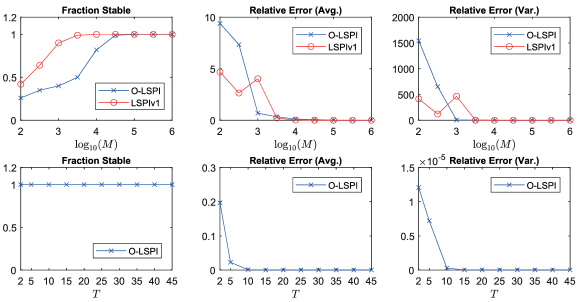
Figure 1: Experimental evaluation on the dynamics of (Krauth, Tu, and Recht 2019).

Finally, the performance of O-LSPI and LSPIv1 with various choices of exploration variance $\sigma^{2}_{u}$ has been investigated on the same example (see Appendix F). The performance of both O-LSPI and LSPIv1 is best when the exploration variances are large ($\sigma^{2}_{u}\geq 10$). The performance of both O-LSPI and LSPIv1 deteriorates when the exploration noise variances are medium and small ($\sigma^{2}_{u}<10$). And O-LSPI performs better than LSPIv1 when the exploration noise variances are small ($\sigma^{2}_{u}\leq 10^{-5}$).

Related Work

The investigation of the robustness of policy iteration for problems with continuous state/control spaces is available in previous literature. In (Bertsekas 1995, Proposition 3.6), for discounted optimal control problems of discrete-time systems, it is reported that

$$\limsup_{i\rightarrow\infty}\max_{x\in\mathbb{X}\subset\mathbb{R}^{n}}\left(J_{\mu^{i}}(x)-J^{*}(x)\right)\leq\frac{\epsilon+2\alpha\delta}{(1-\alpha)^{2}},$$ (25)

where $\mu^{i}$ is the policy generated in $i$th iteration, $\delta$ and $\epsilon$ are the upper bounds of the errors in policy evaluation and policy improvement respectively, $0<\alpha<1$ is the discount factor. Bound (25) and our bound in Theorem 2 have the similar styles. However, in our setting the discount factor is $\alpha=1$ so our bound cannot be implied by (25). Utilizing the fact that Riccati operator is contractive in Thompson’s part metric (Thompson 1963), it is shown in (Krauth, Tu, and Recht 2019, Appendix B) that the convergence to the optimal solutions is still achieved in Thompson’s part metric, if the errors converge to zero. But it is unclear if this result could imply Theorem 2 in this paper. Sufficient conditions on the errors are given in (Hylla 2011, Chapter 2) and (Boussios 1998, Chapter 2) for continuous-time linear and nonlinear system dynamics respectively, to guarantee that the newly generated control policy is stabilizing and improved. The robustness analysis in this paper is parallel to that in (Pang, Bian, and Jiang 2020). However, since we are dealing with discrete-time systems here, the derivations and proofs are inevitably distinct.

In recent years, there have been resurgent research interests in LQR problems, about learning the optimal solutions from the input/state/output data. The model-based certainty equivalence methods explicitly estimate the values of $A$, $B$ and $C$ in (8) from data, and obtain near-optimal solutions based on the estimations, see (Abbasi-Yadkori and Szepesvári 2011; Ouyang, Gagrani, and Jain 2017; Abeille and Lazaric 2018; Dean et al. 2018; Shirani Faradonbeh, Tewari, and Michailidis 2020; Umenberger and Schön 2020; Cassel, Cohen, and Koren 2020; Basei, Guo, and Hu 2020), to name a few. The model-free methods aim at finding the near-optimal solutions directly from the data, without the estimations of system dynamics. Action-value model-free methods learn the value functions of policies, and then generate new (improved) policies based on the estimated value functions, see (Bradtke, Ydstie, and Barto 1994; Tu and Recht 2018; Krauth, Tu, and Recht 2019; Abbasi-Yadkori, Lazic, and Szepesvári 2019; Tu and Recht 2019; Bian and Jiang 2019). Policy-gradient model-free methods directly learn the policies based on the gradient of some scalar performance measure with respect to the policy parameter, see (Fazel et al. 2018; Bu et al. 2019; Preiss et al. 2019; Mohammadi et al. 2019; Yang et al. 2019; Qu et al. 2020; Jansch-Porto, Hu, and Dullerud 2020a, b; Furieri, Zheng, and Kamgarpour 2020). Derivative-free model-free methods randomly search in the parameter space of policies for the near-optimal solutions, without explicitly estimate the gradient, see (Mania, Guy, and Recht 2018; Malik et al. 2019; Li et al. 2020).

Most of the model-free methods for LQR mentioned above are on-policy, fewer theoretical results exist for off-policy methods. Among the off-policy action-value model-free methods for LQR, the most related to our proposed O-LSPI are the LSPIv1 in (Krauth, Tu, and Recht 2019) and the MFLQv1 in (Abbasi-Yadkori, Lazic, and Szepesvári 2019). However, (a) no convergence result is reported for LSPIv1 in (Krauth, Tu, and Recht 2019), and (b) MFLQv1 in (Abbasi-Yadkori, Lazic, and Szepesvári 2019) needs to learn the $P_{K}$ in (5) first in on-policy fashion, before it can learn the $Q(P_{K})$ in (19) in off-policy fashion in each iteration, and (c) both the LSPIv1 and MFLQv1 need the knowledge of matrix $C$ in (8), and (d) both the LSPIv1 and MFLQv1 need to solve a pseudo-inverse problem in each iteration. In contrast, in our O-LSPI, (a) a convergence result is given (Theorem 3), and (b) both the $P_{K}$ and $Q(P_{K})$ are learned in off-policy fashion (Lines 1 to 1 in Algorithm 1), and (c) no knowledge of $C$ is required, and (d) the pseudo-inverse problem only needs to be solved once.

Finally, it is worth mentioning again that the robustness of RL to errors in the learning processes is analyzed in this paper. This is different from the the robustness of the controllers learned by RL to disturbances in the system dynamics, studied in (Gravell, Mohajerin Esfahani, and Summers 2020; Zhang, Hu, and Basar 2020a, b; Turchetta, Krause, and Trimpe 2020; Jiang and Jiang 2017). We also notice that using control theory to study RL algorithms, as we did in this paper, has become popular recently. By regarding the learning processes as dynamical systems, abundant results and techniques in control theory can be applied to obtain better understanding of RL algorithms, see (Srikant and Ying 2019; Gupta, Srikant, and Ying 2019; Hu and Syed 2019; Lee and He 2019; Bian and Jiang 2019).

Concluding Remarks

This paper analyzes the robustness of policy iteration for discrete-time LQR. It is proved that starting from any stabilizing initial policy, the solutions generated by policy iteration with errors are bounded and ultimately enter and stay in a neighbourhood of the optimal solution, as long as the errors are small and bounded. This result in the spirit of small-disturbance input-to-state stability is employed to prove the convergence of the optimistic least-squares policy iteration (O-LSPI), a novel off-policy model-free RL algorithm for discrete-time LQR with additive stochastic noises in the dynamics. The theoretical results are verified by the experiments on a numerical example.

Appendix A Appendix A: Useful auxiliary results

Some useful properties of $\mathcal{L}_{X}(\cdot)$ are provided below.

Lemma 3.

Suppose $X\in\mathbb{R}^{n\times n}$ is stable.

1. For each $Z\in\mathbb{R}^{n\times n}$, if $Y\in\mathbb{S}^{n}$ is the solution of equation $\mathcal{L}_{X}(Y)=-Z$, then

   $$Y=\sum_{k=0}^{\infty}(X^{T})^{k}ZX^{k}.$$

2. $\mathcal{L}_{X}(Y_{1})\leq\mathcal{L}_{X}(Y_{2})\implies Y_{1}\geq Y_{2}$, where $Y_{1},Y_{2}\in\mathbb{S}^{n}$.

Proof.

(i) can be found in (Hewer 1971). For (ii), let $x$ be the solution of system $x_{k+1}=Xx_{k}$, $x(0)=x_{0}$. Then $x_{k}=X^{k}x_{0}$ and by (i)

$$x_{0}^{T}Y_{1}x_{0}=\sum_{k=0}^{\infty}x_{k}^{T}(-\mathcal{L}_{X}(Y_{1}))x_{k}\geq\sum_{k=0}^{\infty}x_{k}^{T}(-\mathcal{L}_{X}(Y_{2}))x_{k}=x_{0}^{T}Y_{2}x_{0}.$$

$x_{0}$ is arbitrary, thus $Y_{1}\geq Y_{2}$. ∎

When Definition 1 is truncated to the linear dynamical system (1), since $x^{*}=0$, we have the following definition.

Definition 4.

System $x_{k+1}=Zx_{k}$ is exponentially stable if for some $a>0$ and $0<b<1$,

$$\|Z^{k}\|_{2}\leq ab^{k}.$$

Definition 4 is equivalent to the $(\tau,\rho)$-stability defined in (Krauth, Tu, and Recht 2019, Definition 1), and is closely related to the strong stability defined in (Cassel, Cohen, and Koren 2020, Definition 5).

Lemma 4 ((Agarwal 2000, Remark 5.5.3.)).

System $x_{k+1}=Zx_{k}$ is stable if and only if it is exponentially stable.

Generally in Definition 4, $a$ and $b$ depend on the choice of matrix $Z$. The next lemma shows that a set of (exponentially) stable systems can share the same constants $a$ and $b$.

Lemma 5.

Let $\mathcal{Z}$ be a compact set of stable matrices, then there exist an $a_{0}>0$ and a $0<b_{0}<1$, such that

$$\|Z^{k}\|_{2}\leq a_{0}b_{0}^{k},\quad\forall k\in\mathbb{Z}_{+}$$

for any $Z\in\mathcal{Z}$.

Proof.

For each $Z\in\mathcal{Z}$, by (Tu and Recht 2019, Lemma B.1) there exist $r>0$, $a>0$ and $0<b<1$, such that

$$\|Z^{\prime k}\|_{2}\leq ab^{k},\quad\forall k\in\mathbb{Z}_{+}$$

for all $\|Z^{\prime}-Z\|_{2}<r$. Then the compactness of $\mathcal{Z}$ completes the proof. ∎

The following lemma provides the relationship between operations $\operatorname{vec}(\cdot)$ and $\operatorname{svec}(\cdot)$.

Lemma 6 ((Magnus and Neudecker 2007, Page 57)).

For $X\in\mathbb{S}^{n}$, there exists a unique matrix $D_{n}\in\mathbb{R}^{n^{2}\times\frac{1}{2}n(n+1)}$ with full column rank, such that

$$\operatorname{vec}(X)=D_{n}\operatorname{svec}(X),\quad\operatorname{svec}(X)=D_{n}^{\dagger}\operatorname{vec}(X).$$

$D_{n}$ is called the duplication matrix.

For $X\in\mathbb{R}^{n\times n}$, $Y\in\mathbb{R}^{n\times m}$, $X+\Delta X\in\mathbb{R}^{n\times n}$, $Y+\Delta Y\in\mathbb{R}^{n\times m}$, supposing $X$ and $X+\Delta X$ are invertible, the following inequality is repeatedly used

$$\begin{split}&\|X^{-1}Y-(X+\Delta X)^{-1}(Y+\Delta Y)\|_{F}=\left\|X^{-1}Y-X^{-1}(Y+\Delta Y)\right.\\ &\left.+X^{-1}(Y+\Delta Y)-(X+\Delta X)^{-1}(Y+\Delta Y)\right\|_{F}\\ &=\|-X^{-1}\Delta Y+X^{-1}\Delta X(X+\Delta X)^{-1}(Y+\Delta Y)\|_{F}\\ &\leq\|X^{-1}\|_{F}\|\Delta Y\|_{F}+\|X^{-1}\|_{F}\|(X+\Delta X)^{-1}\|_{F}\|(Y+\Delta Y)\|_{F}\|\Delta X\|_{F}\end{split}$$ (26)

Appendix B Appendix B: Proof of Lemma 1

Since $\mathcal{A}(\mathscr{K}(P^{*}))$ is stable, by continuity there always exists a $\bar{\delta}_{0}>0$, such that $\mathscr{R}(P_{i})$ is invertible, $\mathcal{A}(\mathscr{K}(P_{i}))$ is stable for all $P_{i}\in\mathcal{\bar{B}}_{\bar{\delta}_{0}}(P^{*})$. Suppose $P_{i}\in\mathcal{\bar{B}}_{\bar{\delta}_{0}}(P^{*})$. Subtracting

$$K_{i+1}^{T}B^{T}P^{*}A+A^{T}P^{*}BK_{i+1}-K_{i+1}^{T}\mathscr{R}(P^{*})K_{i+1}$$

from both sides of the ARE (4) for $P=P^{*}$ and noticing that $K_{i+1}=\mathscr{K}(P_{i})$, we have

$$\begin{split}&\mathcal{L}_{\mathcal{A}(\mathscr{K}(P_{i}))}(P^{*})=-S-\mathscr{K}^{T}(P_{i})R\mathscr{K}(P_{i})+\\ &(\mathscr{K}(P_{i})-\mathscr{K}(P^{*}))^{T}\mathscr{R}(P^{*})(\mathscr{K}(P_{i})-\mathscr{K}(P^{*})).\end{split}$$ (27)

Subtracting (27) from (13), we have

$$\begin{split}P_{i+1}-P^{*}=\mathcal{L}^{-1}_{\mathcal{A}(\mathscr{K}(P_{i}))}\left(((\mathscr{K}(P_{i})-\mathscr{K}(P^{*}))^{T}\mathscr{R}(P^{*})(\mathscr{K}(P_{i})-\mathscr{K}(P^{*}))\right).\end{split}$$

Taking norm on both sides of above equation, (12) yields

$$\begin{split}\|P_{i+1}-P^{*}\|_{F}\leq\|\mathscr{A}(\mathcal{A}(\mathscr{K}(P_{i})))^{-1}\|_{2}\|\mathscr{R}(P^{*})\|_{F}\|\mathscr{K}(P_{i})-\mathscr{K}(P^{*})\|_{F}^{2}.\end{split}$$

Since $\mathscr{K}(\cdot)$ is locally Lipschitz continuous at $P^{*}$, by continuity of matrix norm and matrix inverse, there exists a $c_{1}>0$, such that

$$\|P_{i+1}-P^{*}\|_{F}\leq c_{1}\|P_{i}-P^{*}\|_{F}^{2},\quad\forall P_{i}\in\mathcal{\bar{B}}_{\bar{\delta}_{0}}(P^{*}).$$

So for any $0<\sigma<1$, there exists a $\bar{\delta}_{0}\geq\delta_{0}>0$ with $c_{1}\delta_{0}\leq\sigma$. This completes the proof.

Appendix C Appendix C: Proof of Lemma 2

Before proving Lemma 2, we firstly prove some auxiliary lemmas. The Procedure 2 will exhibit a singularity, if $[\hat{G}_{i}]_{uu}$ in (11) is singular, or the cost (2) of $\hat{K}_{i+1}$ is infinity. The following lemma shows that if $\Delta G_{i}$ is small, no singularity will occur. Let $\bar{\delta}_{0}$ be the one defined in the proof of Lemma 1, then $\delta_{0}\leq\bar{\delta}_{0}$.

Lemma 7.

There exists a $d(\delta_{0})>0$ such that for all $\tilde{P}_{i}\in\mathcal{B}_{\delta_{0}}(P^{*})$, $\hat{K}_{i+1}$ is stabilizing and $[\hat{G}_{i}]_{uu}$ is invertible, if $\|\Delta G_{i}\|_{F}\leq d$.

Proof.

Since $\mathcal{\bar{B}}_{\bar{\delta}_{0}}(P^{*})$ is compact and $\mathcal{A}(\mathscr{K}(\cdot))$ is a continuous function, set

$$\mathcal{S}=\{\mathcal{A}(\mathscr{K}(\tilde{P}_{i}))|\tilde{P}_{i}\in\mathcal{\bar{B}}_{\bar{\delta}_{0}}(P^{*})\}$$

is also compact. By continuity, for each $X\in\mathcal{S}$, there exists a $r(X)>0$ such that any $Y\in\mathcal{B}_{r(X)}(X)$ is stable. The compactness of $\mathcal{S}$ implies the existence of a $\underline{r}>0$, such that each $Y\in\mathcal{B}_{\underline{r}}(X)$ is stable for all $X\in\mathcal{S}$. Similarly, there exists $d_{1}>0$ such that $[\hat{G}_{i}]_{uu}$ is invertible for all $\tilde{P}_{i}\in\mathcal{\bar{B}}_{\bar{\delta}_{0}}(P^{*})$, if $\|\Delta G_{i}\|_{F}\leq d_{1}$. Note that in policy improvement step of Procedure 1 (the policy update step in Procedure 2), the improved policy $\tilde{K}_{i+1}=[\tilde{G}_{i}]_{uu}^{-1}[\tilde{G}_{i}]_{ux}$ (the updated policy $\hat{K}_{i+1}$) is continuous function of $\tilde{G}_{i}$ ($\hat{G}_{i}$), and there exists a $0<d_{2}\leq d_{1}$, such that $\mathcal{A}(\hat{K}_{i+1})\in\mathcal{B}_{\underline{r}}(\mathcal{A}(\mathscr{K}(\tilde{P}_{i})))$ for all $\tilde{P}_{i}\in\mathcal{\bar{B}}_{\bar{\delta}_{0}}(P^{*})$, if $\|\Delta G_{i}\|_{F}\leq d_{2}$. Thus $\hat{K}_{i+1}$ is stabilizing. Setting $d=d_{2}$ completes the proof. ∎

By Lemma 7, if $\|\Delta G_{i}\|_{\infty}\leq d$, then the sequence $\{\tilde{P}_{i}\}_{i=0}^{\infty}$ satisfies (15). For simplicity, we denote $\mathcal{E}(\tilde{G}_{i},\Delta G_{i})$ in (15) by $\mathcal{E}_{i}$. The following lemma gives an upper bound on $\|\mathcal{E}_{i}\|_{F}$ in terms of $\|\Delta G_{i}\|_{F}$.

Lemma 8.

For any $\tilde{P}_{i}\in\mathcal{B}_{\delta_{0}}(P^{*})$ and any $c_{2}>0$, there exists a $0<\delta_{1}^{1}(\delta_{0},c_{2})\leq d$, independent of $\tilde{P}_{i}$, where $d$ is defined in Lemma 7, such that

$$\|\mathcal{E}_{i}\|_{F}\leq c_{3}\|\Delta G_{i}\|_{F}<c_{2},$$

if $\|\Delta G_{i}\|_{F}<\delta_{1}^{1}$, where $c_{3}(\delta_{0})>0$.

Proof.

For any $\tilde{P}_{i}\in\bar{\mathcal{B}}_{\delta_{0}}(P^{*})$, $\|\Delta G_{i}\|_{F}\leq d$, we have from (26)

$$\|\mathscr{K}(\tilde{P}_{i})-\hat{K}_{i+1}\|_{F} \leq\|[\tilde{G}_{i}]^{-1}_{uu}\|_{F}\|\Delta G_{i}\|_{F}+\|[\hat{G}_{i}]^{-1}_{uu}\|_{F}\|[\tilde{G}_{i}]^{-1}_{uu}\|_{F}\|[\hat{G}_{i}]_{ux}\|_{F}\|\Delta G_{i}\|_{F}$$

$$\leq c_{4}(\delta_{0},d)\|\Delta G_{i}\|_{F},$$ (28)

where the last inequality comes from the continuity of matrix inverse and the extremum value theorem. Define

$$\begin{split}\check{P}_{i}=\mathcal{L}_{\mathcal{A}(\hat{K}_{i+1})}^{-1}\left(-S-\hat{K}^{T}_{i+1}R\hat{K}_{i+1}\right),\quad\mathring{P}_{i}=\mathcal{L}_{\mathcal{A}(\mathscr{K}(\tilde{P}_{i}))}^{-1}\left(-S-\mathscr{K}(\tilde{P}_{i})^{T}R\mathscr{K}(\tilde{P}_{i})\right).\end{split}$$

Then by (12) and (15),

$$\begin{split}\|\mathcal{E}_{i}\|_{F}&=\|\operatorname{vec}(\check{P}_{i}-\mathring{P}_{i})\|_{2}\\ \operatorname{vec}(\check{P}_{i})&=\mathscr{A}^{-1}\left(\mathcal{A}(\hat{K}_{i+1})\right)\operatorname{vec}\left(-S-\hat{K}^{T}_{i+1}R\hat{K}_{i+1}\right)\\ \operatorname{vec}(\mathring{P}_{i})&=\mathscr{A}^{-1}\left(\mathcal{A}(\mathscr{K}(\tilde{P}_{i}))\right)\operatorname{vec}\left(-S-\mathscr{K}(\tilde{P}_{i})^{T}R\mathscr{K}(\tilde{P}_{i})\right).\end{split}$$

Define

$$\begin{split}\Delta\mathscr{A}_{i}&=\mathscr{A}\left(\mathcal{A}(\mathscr{K}(\tilde{P}_{i}))\right)-\mathscr{A}\left(\mathcal{A}(\hat{K}_{i+1})\right),\quad\Delta b_{i}=\operatorname{vec}\left(\mathscr{K}(\tilde{P}_{i})^{T}R\mathscr{K}(\tilde{P}_{i})-\hat{K}_{i+1}^{T}R\hat{K}_{i+1}\right).\end{split}$$

Using (28), it is easy to check that $\|\Delta\mathscr{A}_{i}\|_{F}\leq c_{5}\|\Delta G_{i}\|_{F}$, $\|\Delta b_{i}\|_{2}\leq c_{6}\|\Delta G_{i}\|_{F}$, for some $c_{5}(\delta_{0},d)>0$, $c_{6}(\delta_{0},d)>0$. Then by (26)

$$\begin{split}\|\mathcal{E}_{i}\|_{F}&\leq\left\|\mathscr{A}^{-1}\left(\mathcal{A}(\hat{K}_{i+1})\right)\right\|_{F}\left(c_{6}+c_{5}\left\|\mathscr{A}^{-1}\left(\mathcal{A}(\mathscr{K}(\tilde{P}_{i}))\right)\right\|_{F}\right.\\ &\left.\times\left\|S+\mathscr{K}(\tilde{P}_{i})^{T}R\mathscr{K}(\tilde{P}_{i})\right\|_{F}\right)\|\Delta G_{i}\|_{F}\\ &\leq c_{3}(\delta_{0})\|\Delta G_{i}\|_{F}\end{split}$$

where the last inequality comes from the continuity of matrix inverse and Lemma 7. Choosing $0<\delta^{1}_{1}\leq d$ such that $c_{3}\delta^{1}_{1}<c_{2}$ completes the proof.

∎

Now we are ready to prove Lemma 2.

Proof of Lemma 2.

Let $c_{2}=(1-\sigma)\delta_{0}$ in Lemma 8, and $\delta_{1}$ be equal to the $\delta_{1}^{1}$ associated with $c_{2}$. For any $i\in\mathbb{Z}_{+}$, if $\tilde{P}_{i}\in\mathcal{B}_{\delta_{0}}(P^{*})$, then $[\hat{G}_{i}]_{uu}$ is invertible, $\hat{K}_{i+1}$ is stabilizing and

$$\|\tilde{P}_{i+1}-P^{*}\|_{F} \leq\|\mathcal{E}_{i}\|_{F}+\left\|\mathcal{L}^{-1}_{\mathcal{A}(\mathscr{K}(\tilde{P}_{i}))}(S+\tilde{P}^{T}_{i}BR^{-1}B^{T}\tilde{P}_{i})-P^{*}\right\|_{F}$$

$$\leq\sigma\|\tilde{P}_{i}-P^{*}\|_{F}+c_{3}\|\Delta G_{i}\|_{F}$$ (29)

$$\leq\sigma\|\tilde{P}_{i}-P^{*}\|_{F}+c_{3}\|\Delta G\|_{\infty}$$ (30)

$$<\sigma\delta_{0}+c_{3}\delta_{1}<\sigma\delta_{0}+c_{2}=\delta_{0},$$ (31)

where (29) and (31) are due to Lemmas 1 and 8. By induction, (29) to (31) hold for all $i\in\mathbb{Z}_{+}$, thus by (30),

$$\begin{split}\|\tilde{P}_{i}-P^{*}\|_{F}&\leq\sigma^{2}\|\tilde{P}_{i-2}-P^{*}\|_{F}+(\sigma+1)c_{3}\|\Delta G\|_{\infty}\\ &\leq\cdots\leq\sigma^{i}\|\tilde{P}_{0}-P^{*}\|_{F}+(1+\cdots+\sigma^{i-1})c_{3}\|\Delta G\|_{\infty}\\ &<\sigma^{i}\|\tilde{P}_{0}-P^{*}\|_{F}+\frac{c_{3}}{1-\sigma}\|\Delta G\|_{\infty},\end{split}$$

which proves (i) and (ii) in Lemma 2. Then (28) implies (iii) in Lemma 2.

In terms of (iv) in Lemma 2, for any $\epsilon>0$, there exists a $i_{1}\in\mathbb{Z}_{+}$, such that $\sup\{\|\Delta G_{i}\|_{F}\}_{i=i_{1}}^{\infty}<\gamma^{-1}(\epsilon/2)$. Take $i_{2}\geq i_{1}$. For $i\geq i_{2}$, we have by (ii) in Lemma 2,

$$\begin{split}\|\tilde{P}_{i}-P^{*}\|_{F}\leq\beta(\|\tilde{P}_{i_{2}}-P^{*}\|_{F},i-i_{2})+\epsilon/2\leq\beta(c_{7},i-i_{2})+\epsilon/2.\end{split}$$

where the second inequality is due to the boundedness of $\tilde{P}_{i}$. Since $\lim_{i\rightarrow\infty}\beta(c_{7},i-i_{2})=0$, there is a $i_{3}\geq i_{2}$ such that $\beta(c_{7},i-i_{2})<\epsilon/2$ for all $i\geq i_{3}$, which completes the proof. ∎

Appendix D Appendix D: Proof of Theorem 2

Notice that all the conclusions of Theorem 2 can be implied by Lemma 2 if

$$\delta_{2}<\min(\gamma^{-1}(\epsilon),\delta_{1}),\quad\tilde{P}_{1}\in\mathcal{B}_{\delta_{0}}(P^{*})$$

for Procedure 2. Thus the proof of Theorem 2 reduces to the proof of the following lemma.

Lemma 9.

Given a stabilizing $\hat{K}_{1}$, there exist $0<\delta_{2}<\min(\gamma^{-1}(\epsilon),\delta_{1})$, $\bar{i}\in\mathbb{Z}_{+}$, $\Pi_{2}>0$ and $\kappa_{2}>0$, such that $[\hat{G}_{i}]_{uu}$ is invertible, $\hat{K}_{i}$ is stabilizing, $\|\tilde{P}_{i}\|_{F}<\Pi_{2}$, $\|\hat{K}_{i}\|_{F}<\kappa_{2}$, $i=1,\cdots,\bar{i}$, $\tilde{P}_{\bar{i}}\in\mathcal{B}_{\delta_{0}}(P^{*})$, as long as $\|\Delta G\|_{\infty}<\delta_{2}$.

The next two lemmas, inspired by (Abbasi-Yadkori, Lazic, and Szepesvári 2019, Lemma 5.1), state that under certain conditions on $\|\Delta G_{i}\|_{F}$, each element in $\{\hat{K}_{i}\}_{i=1}^{\bar{i}}$ is stabilizing, each element in $\{[\hat{G}_{i}]_{uu}\}_{i=1}^{\bar{i}}$ is invertible and $\{\tilde{P}_{i}\}_{i=1}^{\bar{i}}$ is bounded. For simplicity, in the following we assume $S>I_{n}$ and $R>I_{m}$. All the proofs still work for any $S>0$ and $R>0$, by suitable rescaling.

Lemma 10.

If $\hat{K}_{i}$ is stabilizing, then $[\hat{G}_{i}]_{uu}$ is nonsingular and $\hat{K}_{i+1}$ is stabilizing, as long as $\|\Delta G_{i}\|_{F}<a_{i}$, where

$$a_{i}=\left(m(\sqrt{n}+\|\hat{K}_{i}\|_{2})^{2}+m(\sqrt{n}+\|\hat{K}_{i+1}\|_{2})^{2}\right)^{-1}.$$

Furthermore,

$$\|\hat{K}_{i+1}\|_{F}\leq 2\|R^{-1}\|_{F}(1+\|B^{T}\tilde{P}_{i}A\|_{F}).$$ (32)

Proof.

By definition,

$$\|[\tilde{G}_{i}]_{uu}^{-1}([\hat{G}_{i}]_{uu}-[\tilde{G}_{i}]_{uu})\|_{F}<a_{i}\|[\tilde{G}_{i}]_{uu}^{-1}\|_{F}.$$

Since $R>I_{m}$, the eigenvalues $\lambda_{j}([\tilde{G}_{i}]_{uu}^{-1})\in(0,1]$ for all $1\leq j\leq m$. Then by the fact that for any $X\in\mathbb{S}^{m}$

$$\|X\|_{F}=\|\Lambda_{X}\|_{F},\quad\Lambda_{X}=\mathrm{diag}\{\lambda_{1}(X),\cdots,\lambda_{m}(X)\},$$

we have

$$\|[\tilde{G}_{i}]_{uu}^{-1}([\hat{G}_{i}]_{uu}-[\tilde{G}_{i}]_{uu})\|_{F}<a_{i}\sqrt{m}<0.5.$$ (33)

Thus by (Horn and Johnson 2012, Section 5.8), $[\hat{G}_{i}]_{uu}$ is invertible.

For any $x\in\mathbb{R}^{n}$ on the unit ball, define

$$\mathcal{X}_{\hat{K}_{i}}=\left[\begin{array}[]{c}I\\ -\hat{K}_{i}\end{array}\right]xx^{T}\left[\begin{array}[]{cc}I&-\hat{K}_{i}^{T}\end{array}\right].$$

From (10) and (11) we have

$$x^{T}\mathcal{H}(\tilde{G}_{i},\hat{K}_{i})x=\tr(\tilde{G}_{i}\mathcal{X}_{\hat{K}_{i}})=0,$$

and

$$\tr(\hat{G}_{i}\mathcal{X}_{\hat{K}_{i+1}})=\min_{K\in\mathbb{R}^{m\times n}}\tr(\hat{G}_{i}\mathcal{X}_{K}).$$

Then

$$\mathrm{tr}(\tilde{G}_{i}\mathcal{X}_{\hat{K}_{i+1}})\leq\mathrm{tr}(\hat{G}_{i}\mathcal{X}_{\hat{K}_{i+1}})+\|\Delta G_{i}\|_{F}\mathrm{tr}(\mathbf{1}\mathbf{1}^{T}|\mathcal{X}_{\hat{K}_{i+1}}|_{abs})$$

$$\leq\mathrm{tr}(\hat{G}_{i}\mathcal{X}_{\hat{K}_{i}})+\|\Delta G_{i}\|_{F}\mathbf{1}^{T}|\mathcal{X}_{\hat{K}_{i+1}}|_{abs}\mathbf{1}$$

$$\leq\mathrm{tr}(\tilde{G}_{i}\mathcal{X}_{\hat{K}_{i}})+\|\Delta G_{i}\|_{F}\mathbf{1}^{T}(|\mathcal{X}_{\hat{K}_{i}}|_{abs}+|\mathcal{X}_{\hat{K}_{i+1}}|_{abs})\mathbf{1}$$

$$\leq\|\Delta G_{i}\|_{F}\mathbf{1}^{T}(|\mathcal{X}_{\hat{K}_{i}}|_{abs}+|\mathcal{X}_{\hat{K}_{i+1}}|_{abs})\mathbf{1},$$ (34)

where $|\mathcal{X}_{\hat{K}_{i}}|_{abs}$ denotes the matrix obtained from $\mathcal{X}_{\hat{K}_{i}}$ by taking the absolute value of each entry. Thus by (34) and the definition of $\tilde{G}_{i}$, we have

$$x^{T}\mathcal{L}_{\mathcal{A}(\hat{K}_{i+1})}(\tilde{P}_{i})x+\epsilon_{1}\leq 0$$ (35)

where

$$\begin{split}\epsilon_{1}=x^{T}(S+\hat{K}_{i+1}^{T}R\hat{K}_{i+1})x-\|\Delta G_{i}\|_{F}\mathbf{1}^{T}(|\mathcal{X}_{\hat{K}_{i}}|_{abs}+|\mathcal{X}_{\hat{K}_{i+1}}|_{abs})\mathbf{1}.\end{split}$$

For any $x$ on the unit ball, $|\mathbf{1}^{T}x|_{abs}\leq\sqrt{n}$. Similarly, for any $K\in\mathbb{R}^{m\times n}$, by the definition of induced matrix norm, $|\mathbf{1}^{T}Kx|_{abs}\leq\|K\|_{2}\sqrt{m}$. This implies

$$\left|\mathbf{1}^{T}\left[\begin{array}[]{c}I\\ -K\end{array}\right]x\right|_{abs}=\left|\mathbf{1}^{T}x-\mathbf{1}^{T}Kx\right|_{abs}\leq\sqrt{m}(\sqrt{n}+\|K\|_{2}),$$

which means $\mathbf{1}^{T}|\mathcal{X}_{K}|_{abs}\mathbf{1}\leq m(\sqrt{n}+\|K\|_{2})^{2}$. Thus

$$\|\Delta G_{i}\|_{F}\mathbf{1}^{T}(|\mathcal{X}_{\hat{K}_{i}}|_{abs}+|\mathcal{X}_{\hat{K}_{i+1}}|_{abs})\mathbf{1}<1.$$

Then $S>I_{n}$ leads to

$$x^{T}\left(\mathcal{A}(\hat{K}_{i+1})^{T}\tilde{P}_{i}\mathcal{A}(\hat{K}_{i+1})-\tilde{P}_{i}\right)x<0$$

for all $x$ on the unit ball. So $\hat{K}_{i+1}$ is stabilizing by the Lyapunov criterion (Wonham 1985, Lemma $12.2^{\prime}$).

By definition,

$$\|\hat{K}_{i+1}\|_{F} \leq\|[\hat{G}_{i}]_{uu}^{-1}\|_{F}(1+\|B^{T}\tilde{P}_{i}A\|_{F})$$

$$\leq\|[\tilde{G}_{i}]_{uu}^{-1}\|_{F}(1-\|[\tilde{G}_{i}]_{uu}^{-1}([\hat{G}_{i}]_{uu}-[\tilde{G}_{i}]_{uu})\|_{F})^{-1}(1+\|B^{T}\tilde{P}_{i}A\|_{F})$$

$$\leq 2\|R^{-1}\|_{F}(1+\|B^{T}\tilde{P}_{i}A\|_{F}).$$ (36)

where the second inequality comes from (Horn and Johnson 2012, Inequality (5.8.2)), and the last inequality is due to (33). This completes the proof. ∎

Lemma 11.

For any $\bar{i}\in\mathbb{Z}_{+}$, $\bar{i}>0$, if

$$\|\Delta G_{i}\|_{F}<(1+i^{2})^{-1}a_{i},\quad i=1,\cdots,\bar{i},$$ (37)

where $a_{i}$ is defined in Lemma 10, then

$$\|\tilde{P}_{i}\|_{F}\leq 6\|\tilde{P}_{1}\|_{F},\quad\|\hat{K}_{i}\|_{F}\leq C_{0},$$

for $i=1,\cdots,\bar{i}$, where

$$C_{0}=\max\left\{\|\hat{K}_{1}\|_{F},2\|R^{-1}\|_{F}\left(1+6\|B^{T}\|_{F}\|\tilde{P}_{1}\|_{F}\|A\|_{F}\right)\right\}.$$

Proof.

Inequality (35) yields

$$\mathcal{L}_{\mathcal{A}(\hat{K}_{i+1})}(\tilde{P}_{i})+(S+\hat{K}_{i+1}^{T}R\hat{K}_{i+1})-\epsilon_{2,i}I<0.$$ (38)

where

$$\epsilon_{2,i}=\|\Delta G_{i}\|_{F}\mathbf{1}^{T}(|\mathcal{X}_{\hat{K}_{i}}|_{abs}+|\mathcal{X}_{\hat{K}_{i+1}}|_{abs})\mathbf{1}<1.$$

Inserting (10) into above inequality, and using (ii) in Lemma 3, we have

$$\tilde{P}_{i+1}<\tilde{P}_{i}+\epsilon_{2,i}\mathcal{L}_{\mathcal{A}(\hat{K}_{i+1})}^{-1}(-I).$$ (39)

With $S>I_{n}$, (38) yields

$$\mathcal{L}_{\mathcal{A}(\hat{K}_{i+1})}(\tilde{P}_{i})+(1-\epsilon_{2,i})I<0.$$

Similar to (39), we have

$$\mathcal{L}_{\mathcal{A}(\hat{K}_{i+1})}^{-1}(-I)<\frac{1}{1-\epsilon_{2,i}}\tilde{P}_{i}.$$ (40)

From (39) and (40), we obtain

$$\tilde{P}_{i+1}<\left(1+\frac{\epsilon_{2,i}}{1-\epsilon_{2,i}}\right)\tilde{P}_{i}.$$

By definition of $\epsilon_{2,i}$ and condition (37),

$$\frac{\epsilon_{2,i}}{1-\epsilon_{2,i}}\leq\frac{1}{i^{2}},\quad i=1,\cdots,\bar{i}.$$

Then (Konrad 1990, §28. Theorem 3) yields

$$\tilde{P}_{i}\leq 6\tilde{P}_{1},\quad i=1,\cdots,\bar{i}.$$

An application of (32) completes the proof. ∎

Now we are ready to prove Lemma 9.

Proof of Lemma 9.

Consider Procedure 2 confined to the first $\bar{i}$ iterations, where $\bar{i}$ is a sufficiently large integer to be determined later in this proof. Suppose

$$\|\Delta G_{i}\|_{F}<b_{\bar{i}}\triangleq\frac{1}{2m(1+\bar{i}^{2})}\left(\sqrt{n}+C_{0}\right)^{-2}.$$ (41)

Condition (41) implies condition (37). Thus $\hat{K}_{i}$ is stabilizing, $[\hat{G}_{i}]_{uu}^{-1}$ is invertible, $\|\tilde{P}_{i}\|_{F}$ and $\|\hat{K}_{i}\|_{F}$ are bounded. By (10) we have

$$\begin{split}\mathcal{L}_{\mathcal{A}(\hat{K}_{i+1})}(\tilde{P}_{i+1}-\tilde{P}_{i})&=-S-\hat{K}_{i+1}^{T}R\hat{K}_{i+1}-\mathcal{L}_{\mathcal{A}(\hat{K}_{i+1})}(\tilde{P}_{i}).\end{split}$$

Letting $E_{i}=\hat{K}_{i+1}-\mathscr{K}(\tilde{P}_{i})$, the above equation can be rewritten as

$$\tilde{P}_{i+1}=\tilde{P}_{i}-\mathcal{N}(\tilde{P_{i}})+\mathcal{L}_{\mathcal{A}(\mathscr{K}(\tilde{P_{i}}))}^{-1}(\mathscr{E}_{i}),$$ (42)

where $\mathcal{N}(\tilde{P_{i}})=\mathcal{L}_{\mathcal{A}(\mathscr{K}(\tilde{P_{i}}))}^{-1}\circ\mathcal{R}(\tilde{P}_{i}),$ and

$$\begin{split}\mathcal{R}(Y)&=A^{T}YA-Y-A^{T}YB(R+B^{T}YB)^{-1}B^{T}YA+S,\\ \mathscr{E}_{i}&=-E_{i}^{T}\mathscr{R}(\tilde{P}_{i+1})E_{i}+E_{i}^{T}\mathscr{R}(\tilde{P}_{i+1})\left(\mathscr{K}(\tilde{P}_{i+1})-\mathscr{K}(\tilde{P}_{i})\right)\\ &+\left(\mathscr{K}(\tilde{P}_{i+1})-\mathscr{K}(\tilde{P}_{i})\right)^{T}\mathscr{R}(\tilde{P}_{i+1})E_{i}.\end{split}$$

Given $\hat{K}_{1}$, let $\mathcal{M}_{\bar{i}}$ denote the set of all possible $\tilde{P}_{i}$, generated by (42) under condition (41). By definition, $\{\mathcal{M}_{j}\}_{j=1}^{\infty}$ is a nondecreasing sequence of sets, i.e., $\mathcal{M}_{1}\subset\mathcal{M}_{2}\subset\cdots$. Define $\mathcal{M}=\cup_{j=1}^{\infty}\mathcal{M}_{j}$, $\mathcal{D}=\{P\in\mathbb{S}^{n}\ |\ \|P\|_{F}\leq 6\|\tilde{P}_{1}\|_{F}\}$. Then by Lemma 11 and Theorem 1, $\mathcal{M}\subset\mathcal{D}$; $\mathcal{M}$ is compact; $\mathcal{A}(\mathscr{K}(P))$ is stable for any $P\in\mathcal{M}$.

Now we prove that $\mathcal{N}(\cdot)$ is Lipschitz continuous on $\mathcal{M}$. Using (12), for any $P^{1},P^{2}\in\mathcal{M}$ we have

$$\|\mathcal{N}(P^{1})-\mathcal{N}(P^{2})\|_{F} =\|\mathscr{A}^{-1}(\mathcal{A}(\mathscr{K}(P^{1})))\operatorname{vec}(\mathcal{R}(P^{1}))-\mathscr{A}^{-1}(\mathcal{A}(\mathscr{K}(P^{2})))\operatorname{vec}(\mathcal{R}(P^{2}))\|_{2}$$

$$\leq\|\mathscr{A}^{-1}(\mathcal{A}(\mathscr{K}(P^{1})))\|_{2}\|\mathcal{R}(P^{1})-\mathcal{R}(P^{2})\|_{F}+$$

$$\|\mathcal{R}(P^{2})\|_{F}\|\mathscr{A}^{-1}(\mathcal{A}(\mathscr{K}(P^{1})))-\mathscr{A}^{-1}(\mathcal{A}(\mathscr{K}(P^{2})))\|_{2}$$

$$\leq L\|P^{1}-P^{2}\|_{F}$$ (43)

with some Lipschitz constant $L>0$, where the last inequality is due to the fact that matrix inversion, $\mathcal{A}(\cdot)$, $\mathscr{K}(\cdot)$ and $\mathcal{R}(\cdot)$ are locally Lipschitz, thus Lipschitz on compact set $\mathcal{M}$.

Define $\{P_{k|i}\}_{k=0}^{\infty}$ as the sequence generated by (13) with $P_{0|i}=\tilde{P}_{i}$. Similar to (42), we have

$$P_{k+1|i}=P_{k|i}-\mathcal{N}(P_{k|i}),\quad k\in\mathbb{Z}_{+}.$$ (44)

By Theorem 1 and the fact that $\mathcal{M}$ is compact, there exists $k_{0}\in\mathbb{Z}_{+}$, such that

$$\|P_{k_{0}|i}-P^{*}\|_{F}<\delta_{0}/2,\qquad\forall P_{0|i}\in\mathcal{M}.$$ (45)

Suppose

$$\|\mathcal{L}_{\mathcal{A}(\mathscr{K}(\tilde{P}_{i+j}))}^{-1}(\mathscr{E}_{i+j})\|_{F}<\mu,\qquad j=0,\cdots,\bar{i}-i.$$ (46)

We find an upper bound on $\|P_{k|i}-\tilde{P}_{i+k}\|_{F}$. Notice that from (42) and (44),

$$\begin{split}P_{k|i}=P_{0|i}-\sum_{j=0}^{k-1}\mathcal{N}(P_{j|i}),\qquad\tilde{P}_{i+k}=\tilde{P}_{i}-\sum_{j=0}^{k-1}\mathcal{N}(\tilde{P}_{i+j})+\sum_{j=0}^{k-1}\mathcal{L}_{\mathcal{A}(\mathscr{K}(\tilde{P}_{i+j}))}^{-1}(\mathscr{E}_{i+j}).\end{split}$$

Then (D) and (46) yield

$$\begin{split}\|P_{k|i}-\tilde{P}_{i+k}\|_{F}\leq k\mu+\sum_{j=0}^{k-1}L\|P_{j|i}-\tilde{P}_{i+j}\|_{F}.\end{split}$$

An application of the Gronwall inequality (Agarwal 2000, Theorem 4.1.1.) to the above inequality implies

$$\|P_{k|i}-\tilde{P}_{i+k}\|_{F}\leq k\mu+L\mu\sum_{j=0}^{k-1}j(1+L)^{k-j-1}.$$ (47)

By (i) in Lemma 3,

$$\mathcal{L}^{-1}_{\mathcal{A}(\mathscr{K}(P^{1}))}(-I)=\sum_{k=0}^{\infty}(\mathcal{A}^{T}(\mathscr{K}(P^{1})))^{k}(\mathcal{A}(\mathscr{K}(P^{1})))^{k},\quad P^{1}\in\mathcal{M}.$$

By definition of the set $\mathcal{M}$, there exist $G^{1}$ and stabilizing control gain $K^{1}$ associated with $P^{1}\in\mathcal{M}$, such that $\mathcal{H}(G^{1},K^{1})=0$. So for any $x\in\mathbb{R}^{n}$,

$$x^{T}\mathcal{R}(P^{1})x=\min_{K\in\mathbb{R}^{m\times n}}x^{T}\mathcal{H}(G^{1},K)x\leq 0.$$

This implies

$$\mathcal{L}_{\mathcal{A}(\mathscr{K}(P^{1}))}(P^{1})\leq-S-\mathscr{K}^{T}(P^{1})R\mathscr{K}(P^{1})<-I.$$

An application of (ii) in Lemma 3 to the above inequality leads to

$$\|\mathcal{L}^{-1}_{\mathcal{A}(\mathscr{K}(P^{1}))}(-I)\|_{F}<P^{1}\leq 6\|\tilde{P}_{1}\|_{F},\qquad\forall P^{1}\in\mathcal{M}\subset\mathcal{D}.$$ (48)

Then the error term in (42) satisfies

$$\left\|\mathcal{L}_{\mathcal{A}(\mathscr{K}(\tilde{P_{i}}))}^{-1}(\mathscr{E}_{i})\right\|_{F}=\left\|\sum_{k=0}^{\infty}(\mathcal{A}^{T}(\mathscr{K}(\tilde{P_{i}})))^{k}\otimes(\mathcal{A}(\mathscr{K}(\tilde{P_{i}})))^{k}\operatorname{vec}\left(\mathscr{E}_{i}\right)\right\|_{2}\leq C_{1}\|\mathscr{E}_{i}\|_{F},$$ (49)

where $C_{1}$ is a constant and the inequality is due to (48).

Let $\bar{i}>k_{0}$, and $k=k_{0}$, $i=\bar{i}-k_{0}$ in (47). Then by condition (41), Lemma 11, (46), (47), and (49), there exists $i_{0}\in\mathbb{Z}_{+}$, $i_{0}>k_{0}$, such that $\|P_{k_{0}|\bar{i}-k_{0}}-\tilde{P}_{\bar{i}}\|_{F}<\delta_{0}/2$, for all $\bar{i}\geq i_{0}$. Setting $i=\bar{i}-k_{0}$ in (45), the triangle inequality yields $\tilde{P}_{\bar{i}}\in\mathcal{B}_{\delta_{0}}(P^{*})$, for $\bar{i}\geq i_{0}$. Then in (41), choosing $\bar{i}\geq i_{0}$ such that $\delta_{2}=b_{\bar{i}}<\min(\gamma^{-1}(\epsilon),\delta_{1})$ completes the proof. ∎

Appendix E Appendix E: Proof of Theorem 3

For given $\hat{K}_{1}$, let $\mathcal{F}$ denote the set of control gains (including $\hat{K}_{1}$) generated by Procedure 2 with all possible $\{\Delta G_{i}\}_{i=1}^{\infty}$ satisfying $\|\Delta G\|_{\infty}<\delta_{2}$, where $\delta_{2}$ is the one in Theorem 2. The following result is firstly derived.

Lemma 12.

Under Assumption 1, there exist $T_{0}\in\mathbb{Z}_{+}$ and $M_{0}\in\mathbb{Z}_{+}$, such that for any $T\geq T_{0}$ and any $M\geq M_{0}$, $\hat{K}_{i}\in\mathcal{F}$ implies $\|\Delta G_{i}\|_{F}<\delta_{2}$, almost surely.

Proof.

The task is to show that each term in (23) is less than $\delta_{2}/3$ almost surely.

We firstly study term $\|\hat{P}_{i,T}-\tilde{P}_{i}\|_{F}$. Define $\hat{p}_{i,j}=\operatorname{vec}(\hat{P}_{i,j})$, then by Lemma 6, lines from 1 to 1 in Algorithm 1 can be rewritten as

$$\begin{split}\hat{p}_{i,j+1}&=\operatorname{vec}(\mathcal{H}(\mathcal{H}(\operatorname{svec}^{-1}(\Phi_{M}^{\dagger}\Psi_{M}\operatorname{svec}(\hat{P}_{i,j})+\Phi_{M}^{\dagger}\Xi_{M}),0),\hat{K}_{i}))\\ &=\mathcal{T}^{1}(\Phi_{M},\Psi_{M},\hat{K}_{i})\hat{p}_{i,j}+\mathcal{T}^{2}(\Phi_{M},\Xi_{M},\hat{K}_{i}),\quad\hat{p}_{i,0}=0,\end{split}$$ (50)

where $Y=\operatorname{svec}^{-1}(\operatorname{svec}(Y))$, for any $Y\in\mathbb{S}^{n}$, and

$$\begin{split}\mathcal{T}^{1}(\Phi_{M},\Psi_{M},\hat{K}_{i})&=\left(\left[I_{n},-\hat{K}^{T}_{i}\right]\otimes\left[I_{n},-\hat{K}^{T}_{i}\right]\right)\left(\left[I_{m+n},0\right]\otimes\left[I_{m+n},0\right]\right)D_{m+n+1}\Phi_{M}^{\dagger}\Psi_{M}D_{n}^{\dagger},\\ \mathcal{T}^{2}(\Phi_{M},\Xi_{M},\hat{K}_{i})&=\left(\left[I_{n},-\hat{K}^{T}_{i}\right]\otimes\left[I_{n},-\hat{K}^{T}_{i}\right]\right)\left(\left[I_{m+n},0\right]\otimes\left[I_{m+n},0\right]\right)D_{m+n+1}\Phi_{M}^{\dagger}\Xi_{M}.\end{split}$$

Set $K=\hat{K}_{i}$ and insert (22) into (18). Similar derivations yield

$$\tilde{p}_{i,j+1}=\mathcal{T}^{1}(\varphi_{1},\varphi_{2},\hat{K}_{i})\tilde{p}_{i,j}+\mathcal{T}^{2}(\varphi_{1},\varphi_{3},\hat{K}_{i}),\quad\tilde{p}_{i,0}=0.$$ (51)

By Assumption 1, (51) is identical to

$$\tilde{p}_{i,j+1}=(A-B\hat{K}_{i})^{T}\otimes(A-B\hat{K}_{i})^{T}\tilde{p}_{i,j}+\operatorname{vec}(S+\hat{K}_{i}^{T}R\hat{K}_{i}),\quad\tilde{p}_{i,0}=0,$$ (52)

with

$$\mathcal{T}^{1}(\varphi_{1},\varphi_{2},\hat{K}_{i})=(A-B\hat{K}_{i})^{T}\otimes(A-B\hat{K}_{i})^{T},\quad\mathcal{T}^{2}(\varphi_{1},\varphi_{3},\hat{K}_{i})=\operatorname{vec}(S+\hat{K}_{i}^{T}R\hat{K}_{i}).$$ (53)

Since $\hat{K}_{i}\in\mathcal{F}$ is stabilizing,

$$\lim_{j\rightarrow\infty}\tilde{P}_{i,j}=\tilde{P}_{i}$$ (54)

where $\tilde{p}_{i,j}=\operatorname{vec}(\tilde{P}_{i,j})$ and $\tilde{P}_{i}$ is the unique solution of (5) with $K=\hat{K}_{i}$. By definition and Theorem 2, $\bar{\mathcal{F}}$ is bounded, thus compact. Let $\mathcal{V}$ be the set of unique solutions of (5) with $K\in\mathcal{F}$. Then by Theorem 2 $\mathcal{V}$ is bounded. So any control gain in $\bar{\mathcal{F}}$ is stabilizing, otherwise it contradicts the boundedness of $\mathcal{V}$. Define

$$\mathcal{F}_{1}=\{(A-BK)^{T}\otimes(A-BK)^{T}|K\in\bar{\mathcal{F}}\}.$$

By continuity, $\mathcal{F}_{1}$ is a compact set of stable matrices, and there exists a $\delta_{3}>0$, such that any $X\in\bar{\mathcal{F}}_{2}$ is stable, where

$$\mathcal{F}_{2}=\{X|X\in\mathcal{B}_{\delta_{3}}(Y),Y\in\mathcal{F}_{1}\}.$$

Define

$$\Delta\mathcal{T}^{1}_{M,i}=\mathcal{T}^{1}(\varphi_{1},\varphi_{2},\hat{K}_{i})-\mathcal{T}^{1}(\Phi_{M},\Psi_{M},\hat{K}_{i}),\quad\Delta\mathcal{T}^{2}_{M,i}=\mathcal{T}^{2}(\varphi_{1},\varphi_{3},\hat{K}_{i})-\mathcal{T}^{2}(\Phi_{M},\Xi_{M},\hat{K}_{i}).$$

The boundedness of $\mathcal{F}$, (24) and (53) implies the existence of $M_{1}>0$, such that for any $M\geq M_{1}$, any $\hat{K}_{i}\in\mathcal{F}$, almost surely

$$\mathcal{T}^{1}(\Phi_{M},\Psi_{M},\hat{K}_{i})\in\bar{\mathcal{F}}_{2},\quad\mathcal{T}^{2}(\Phi_{M},\Xi_{M},\hat{K}_{i})<C_{2},$$ (55)

where $C_{2}>0$ is a constant. Then (50) admits a unique stable equilibrium, that is,

$$\lim_{j\rightarrow\infty}\hat{P}_{i,j}=\hat{P}_{i}$$ (56)

for some $\hat{P}_{i}\in\mathbb{S}^{n}$, and from (50), (51), (54) and (56), we have

$$\begin{split}\tilde{p}_{i}&=\operatorname{vec}(\tilde{P}_{i})=\left(I_{n^{2}}-\mathcal{T}^{1}(\varphi_{1},\varphi_{2},\hat{K}_{i})\right)^{-1}\mathcal{T}^{2}(\varphi_{1},\varphi_{3},\hat{K}_{i}),\\ \hat{p}_{i}&=\operatorname{vec}(\hat{P}_{i})=\left(I_{n^{2}}-\mathcal{T}^{1}(\Phi_{M},\Psi_{M},\hat{K}_{i})\right)^{-1}\mathcal{T}^{2}(\Phi_{M},\Xi_{M},\hat{K}_{i}).\end{split}$$

Thus by (26), for any $M\geq M_{1}$, any $\hat{K}_{i}\in\mathcal{F}$, almost surely

$$\|\hat{P}_{i}-\tilde{P}_{i}\|_{F} \leq\left\|\left(I_{n^{2}}-\mathcal{T}^{1}(\varphi_{1},\varphi_{2},\hat{K}_{i})\right)^{-1}\right\|_{F}\left(\|\Delta\mathcal{T}^{2}_{M,i}\|_{2}+\right.$$

$$\left.\left\|\left(I_{n^{2}}-\mathcal{T}^{1}(\Phi_{M},\Psi_{M},\hat{K}_{i})\right)^{-1}\right\|_{F}\left\|\mathcal{T}^{2}(\Phi_{M},\Xi_{M},\hat{K}_{i})\right\|_{2}\|\Delta\mathcal{T}^{1}_{M,i}\|_{F}\right)$$

$$\leq c_{8}\|\Delta\mathcal{T}^{2}_{M,i}\|_{F}+c_{9}\|\Delta\mathcal{T}^{1}_{M,i}\|_{F}$$

where $c_{8}$ and $c_{9}$ are some positive constants, and the last inequality is due to (53), (55) and the fact that $\mathcal{F}_{1}$ and $\bar{\mathcal{F}}_{2}$ are compact sets of stable matrices. Then for any $\epsilon_{1}>0$, the boundedness of $\mathcal{F}$ and (24) implies the existence of $M_{2}\geq M_{1}$, such that for any $M\geq M_{2}$, almost surely

$$\|\hat{P}_{i}-\tilde{P}_{i}\|_{F}<\epsilon_{1}/2,$$ (57)

as long as $\hat{K}_{i}\in\mathcal{F}$. By Lemma 5 and (55), for any $M\geq M_{2}$ and any $\hat{K}_{i}\in\mathcal{F}$,

$$\|\hat{p}_{i,j+1}-\hat{p}_{i}\|_{2}\leq a_{0}b_{0}^{k}\|\hat{p}_{i}\|_{2}\leq a_{1}b_{0}^{k},$$

for some $a_{0}>0$, $1>b_{0}>0$ and $a_{1}>0$. Therefore there exists a $T_{1}>0$, such that for any $T\geq T_{1}$, and any $M\geq M_{2}$, almost surely

$$\|\hat{P}_{i,T}-\hat{P}_{i}\|_{F}<\epsilon_{1}/2,$$ (58)

as long as $\hat{K}_{i}\in\mathcal{F}$. Synthesizing (57) and (58) yields

$$\|\hat{P}_{i,T}-\tilde{P}_{i}\|_{F}<\epsilon_{1},$$ (59)

almost surely for any $T\geq T_{1}$, any $M\geq M_{2}$, as long as $\hat{K}_{i}\in\mathcal{F}$. Since $\epsilon_{1}$ is arbitrary, we can choose $\epsilon_{1}$ such that almost surely

$$\|\hat{P}_{i,T}-\tilde{P}_{i}\|_{F}<\epsilon_{1}\leq\frac{\delta_{2}}{3}.$$

Secondly, for term $\|Q(\hat{P}_{i,T})-Q(\tilde{P}_{i})\|_{F}$, by (59) there exist $T_{2}\geq T_{1}$, $M_{3}\geq M_{2}$, such that almost surely

$$\|Q(\hat{P}_{i,T})-Q(\tilde{P}_{i})\|_{F}<\frac{\delta_{2}}{3}$$

for any $T\geq T_{2}$, any $M\geq M_{3}$, as long as $\hat{K}_{i}\in\mathcal{F}$.

Finally, since $\mathcal{V}$ is bounded, by (59) $\hat{P}_{i,T}$ is also almost surely bounded. Thus from lines 1 to 1 in Algorithm 1, and (24), there exists $M_{4}\geq M_{3}$, such that

$$\|\hat{Q}_{i,T}-Q(\hat{P}_{i,T})\|_{F}<\frac{\delta_{2}}{3}$$

for any $M\geq M_{4}$ and any $T\geq T_{2}$, as long as $\hat{K}_{i}\in\mathcal{F}$.

Setting $T_{0}=T_{2}$ and $M_{0}=M_{4}$ yields $\|\Delta G_{i}\|<\delta_{2}$. ∎

Now we are ready to prove Theorem 3.

Proof.

Since $\hat{K}_{1}\in\mathcal{F}$, Lemma 12 implies $\|\Delta G_{1}\|_{F}<\delta_{2}$ almost surely. By definition, $\hat{K}_{2}\in\mathcal{F}$. Thus $\|\Delta G_{i}\|_{F}<\delta_{2},i=1,2,\cdots$ almost surely by mathematical induction. Then Theorem 2 completes the proof. ∎

Appendix F Appendix F: Experiments (Cont’d)

In the experiments of Figure 2, initial control gain is $\hat{K}_{1}=0_{2\times 3}$, number of policy iterations $N=5$, number of iterations for policy evaluation $T=45$. The three features we use to evaluate the performances of the algorithms (fraction stable, relative error (Avg.) and Relative Error (Var.)) in Figure 2 are computed in the same way to those in Figure 1.

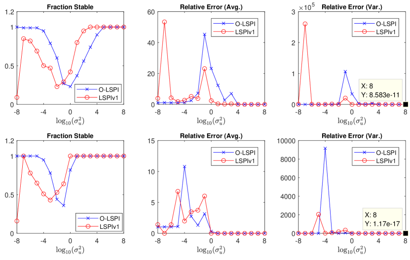
Figure 2: The performances of O-LSPI and LSPIv1 on the dynamics of (Krauth, Tu, and Recht 2019) with different values of exploration variances $\sigma^{2}_{u}$. In the upper row $M=10^{2}$ while in the lower row $M=10^{4}$.

References

• Abbasi-Yadkori and Szepesvári (2011) Abbasi-Yadkori, Y., and Szepesvári, C. 2011. Regret bounds for the adaptive control of linear quadratic systems. In Annual Conference on Learning Theory (COLT), 1–26.
• Abbasi-Yadkori, Lazic, and Szepesvári (2019) Abbasi-Yadkori, Y.; Lazic, N.; and Szepesvári, C. 2019. Model-free linear quadratic control via reduction to expert prediction. In International Conference on Artificial Intelligence and Statistics (AISTATS), 3108–3117.
• Abeille and Lazaric (2018) Abeille, M., and Lazaric, A. 2018. Improved regret bounds for Thompson sampling in linear quadratic control problems. In International Conference on Machine Learning (ICML), 1–9.
• Agarwal (2000) Agarwal, R. P. 2000. Difference Equations and Inequalities: Theory, Methods, and Applications. New York: Marcel Dekker, Inc, 2nd edition.
• Basei, Guo, and Hu (2020) Basei, M.; Guo, X.; and Hu, A. 2020. Linear quadratic reinforcement learning: Sublinear regret in the episodic continuous-time framework. arXiv preprint arXiv:2006.15316.
• Bertsekas (1995) Bertsekas, D. P. 1995. Dynamic Programming and Optimal Control, volume 2. Belmont, MA: Athena Scientific.
• Bertsekas (2011) Bertsekas, D. P. 2011. Approximate policy iteration: A survey and some new methods. Journal of Control Theory and Applications 310–335.
• Bian and Jiang (2019) Bian, T., and Jiang, Z. P. 2019. Continuous-time robust dynamic programming. SIAM Journal on Control and Optimization 4150–4174.
• Boussios (1998) Boussios, C. I. 1998. An approach for nonlinear control design via approximate dynamic programming. Ph.D. Dissertation, Massachusetts Institute of Technology.
• Bradtke, Ydstie, and Barto (1994) Bradtke, S. J.; Ydstie, B. E.; and Barto, A. G. 1994. Adaptive linear quadratic control using policy iteration. In American Control Conference (ACC), 3475–3479.
• Bu et al. (2019) Bu, J.; Mesbahi, A.; Fazel, M.; and Mesbahi, M. 2019. LQR through the lens of first order methods: Discrete-time case. arXiv preprint arXiv:1907.08921.
• Cassel, Cohen, and Koren (2020) Cassel, A.; Cohen, A.; and Koren, T. 2020. Logarithmic regret for learning linear quadratic regulators efficiently. International Conference on Machine Learning (ICML) 1328–1337.
• Dean et al. (2018) Dean, S.; Mania, H.; Matni, N.; Recht, B.; and Tu, S. 2018. Regret bounds for robust adaptive control of the linear quadratic regulator. In Advances in Neural Information Processing Systems (NeurIPS), 4192–4201.
• Fazel et al. (2018) Fazel, M.; Ge, R.; Kakade, S.; and Mesbahi, M. 2018. Global convergence of policy gradient methods for the linear quadratic regulator. In International Conference on Machine Learning (ICML), 1467–1476.
• Furieri, Zheng, and Kamgarpour (2020) Furieri, L.; Zheng, Y.; and Kamgarpour, M. 2020. Learning the globally optimal distributed LQ regulator. In Annual Conference on Learning for Dynamics and Control (L4DC), 287–297.
• Gravell, Mohajerin Esfahani, and Summers (2020) Gravell, B.; Mohajerin Esfahani, P.; and Summers, T. H. 2020. Learning optimal controllers for linear systems with multiplicative noise via policy gradient. IEEE Transactions on Automatic Control.
• Gupta, Srikant, and Ying (2019) Gupta, H.; Srikant, R.; and Ying, L. 2019. Finite-time performance bounds and adaptive learning rate selection for two time-scale reinforcement learning. In Advances in Neural Information Processing Systems (NeurIPS).
• Hewer (1971) Hewer, G. 1971. An iterative technique for the computation of the steady state gains for the discrete optimal regulator. IEEE Transactions on Automatic Control 382–384.
• Horn and Johnson (2012) Horn, R. A., and Johnson, C. R. 2012. Matrix Analysis. New York: Cambridge University Press.
• Hu and Syed (2019) Hu, B., and Syed, U. 2019. Characterizing the exact behaviors of temporal difference learning algorithms using Markov jump linear system theory. In Advances in Neural Information Processing Systems (NeurIPS).
• Hylla (2011) Hylla, T. 2011. Extension of inexact Kleinman-Newton methods to a general monotonicity preserving convergence theory. Ph.D. Dissertation, Universität Trier.
• Jansch-Porto, Hu, and Dullerud (2020a) Jansch-Porto, J. P.; Hu, B.; and Dullerud, G. 2020a. Convergence guarantees of policy optimization methods for Markovian jump linear systems. American Control Conference (ACC) 2882–2887.
• Jansch-Porto, Hu, and Dullerud (2020b) Jansch-Porto, J. P.; Hu, B.; and Dullerud, G. 2020b. Policy learning of MDPs with mixed continuous/discrete variables: A case study on model-free control of Markovian jump systems. Annual Conference on Learning for Dynamics and Control (L4DC) 947–957.
• Jiang and Jiang (2017) Jiang, Y., and Jiang, Z. P. 2017. Robust Adaptive Dynamic Programming. Hoboken, New Jersey: Wiley-IEEE Press.
• Jiang, Bian, and Gao (2020) Jiang, Z.; Bian, T.; and Gao, W. 2020. Learning-based control: A tutorial and some recent results. Foundations and Trends in Systems and Control 176–284.
• Jiang, Lin, and Wang (2004) Jiang, Z. P.; Lin, Y.; and Wang, Y. 2004. Nonlinear small-gain theorems for discrete-time feedback systems and applications. Automatica 2129–2136.
• Konrad (1990) Konrad, K. 1990. Theory and Application of Infinite Series. New York: Dover Publications, 2nd edition.
• Koralov and Sinai (2007) Koralov, L., and Sinai, Y. G. 2007. Theory of Probability and Random Processes. Berlin: Springer, 2nd edition.
• Krauth, Tu, and Recht (2019) Krauth, K.; Tu, S.; and Recht, B. 2019. Finite-time analysis of approximate policy iteration for the linear quadratic regulator. In Advances in Neural Information Processing Systems (NeurIPS).
• Lee and He (2019) Lee, D., and He, N. 2019. A unified switching system perspective and ODE analysis of Q-learning algorithms. arXiv preprint arXiv:1912.02270.
• Levine and Koltun (2012) Levine, S., and Koltun, V. 2012. Continuous inverse optimal control with locally optimal examples. In International Conference on Machine Learning (ICML), 475–482.
• Lewis, Vrabie, and Syrmos (2012) Lewis, F. L.; Vrabie, D.; and Syrmos, V. L. 2012. Optimal Control. Hoboken, New Jersey: John Wiley & Sons.
• Li et al. (2020) Li, Y.; Tang, Y.; Zhang, R.; and Li, N. 2020. Distributed reinforcement learning for decentralized linear quadratic control: A derivative-free policy optimization approach. Annual Conference on Learning for Dynamics and Control (L4DC) 814–814.
• Lillicrap et al. (2016) Lillicrap, T. P.; Hunt, J. J.; Pritzel, A.; Heess, N.; Erez, T.; Tassa, Y.; Silver, D.; and Wierstra, D. 2016. Continuous control with deep reinforcement learning. In International Conference on Learning Representations (ICLR).
• Ljung (1999) Ljung, L. 1999. System Identification: Theory for the user. Upper Saddle River: Prentice Hall PTR, 2nd edition.
• Magnus and Neudecker (2007) Magnus, J. R., and Neudecker, H. 2007. Matrix Differential Calculus With Applications In Statistics And Economerices. New York: Wiley.
• Malik et al. (2019) Malik, D.; Pananjady, A.; Bhatia, K.; Khamaru, K.; Bartlett, P.; and Wainwright, M. 2019. Derivative-free methods for policy optimization: Guarantees for linear quadratic systems. In International Conference on Artificial Intelligence and Statistics (AISTATS), 2916–2925.
• Mania, Guy, and Recht (2018) Mania, H.; Guy, A.; and Recht, B. 2018. Simple random search of static linear policies is competitive for reinforcement learning. In Advances in Neural Information Processing Systems (NeurIPS), 1805–1814.
• Mohammadi et al. (2019) Mohammadi, H.; Zare, A.; Soltanolkotabi, M.; and Jovanović, M. R. 2019. Convergence and sample complexity of gradient methods for the model-free linear quadratic regulator problem. arXiv preprint arXiv:1912.11899.
• Monfort, Liu, and Ziebart (2015) Monfort, M.; Liu, A.; and Ziebart, B. D. 2015. Intent prediction and trajectory forecasting via predictive inverse linear-quadratic regulation. In AAAI Conference on Artificial Intelligence (AAAI), 3672–3678.
• Ouyang, Gagrani, and Jain (2017) Ouyang, Y.; Gagrani, M.; and Jain, R. 2017. Learning-based control of unknown linear systems with Thompson sampling. arXiv preprint arXiv:1709.04047.
• Pang, Bian, and Jiang (2020) Pang, B.; Bian, T.; and Jiang, Z.-P. 2020. Robust policy iteration for continuous-time linear quadratic regulation. arXiv preprint arXiv:2005.09528.
• Preiss et al. (2019) Preiss, J. A.; Arnold, S. M.; Wei, C.-Y.; and Kloft, M. 2019. Analyzing the variance of policy gradient estimators for the linear-quadratic regulator. arXiv preprint arXiv:1910.01249.
• Qu et al. (2020) Qu, G.; Yu, C.; Low, S.; and Wierman, A. 2020. Combining model-based and model-free methods for nonlinear control: A provably convergent policy gradient approach. arXiv preprint arXiv:2006.07476.
• Åström and Wittenmark (1995) Åström, K. J., and Wittenmark, B. 1995. Adaptive Control. Reading, Massachusetts: Addison-Wesley, 2nd edition.
• Shirani Faradonbeh, Tewari, and Michailidis (2020) Shirani Faradonbeh, M. K.; Tewari, A.; and Michailidis, G. 2020. On adaptive linear–quadratic regulators. Automatica.
• Sontag (2008) Sontag, E. D. 2008. Input to state stability: Basic concepts and results. In Nonlinear and optimal control theory, volume 1932. Berlin: Springer. 163–220.
• Srikant and Ying (2019) Srikant, R., and Ying, L. 2019. Finite-time error bounds for linear stochastic approximation and TD learning. In Annual Conference on Learning Theory (COLT), 2803–2830.
• Sutton and Barto (2018) Sutton, R. S., and Barto, A. G. 2018. Reinforcement Learning: An Introduction. Cambridge, Massachusetts: MIT Press, 2nd edition.
• Thompson (1963) Thompson, A. C. 1963. On certain contraction mappings in a partially ordered vector space. Proceedings of the American Mathematical Society 438 – 443.
• Tsitsiklis (2002) Tsitsiklis, J. N. 2002. On the convergence of optimistic policy iteration. Journal of Machine Learning Research 59–72.
• Tu and Recht (2018) Tu, S., and Recht, B. 2018. Least-squares temporal difference learning for the linear quadratic regulator. In International Conference on Machine Learning (ICML), 5005–5014.
• Tu and Recht (2019) Tu, S., and Recht, B. 2019. The gap between model-based and model-free methods on the linear quadratic regulator: An asymptotic viewpoint. In Annual Conference on Learning Theory (COLT), 3036–3083.
• Turchetta, Krause, and Trimpe (2020) Turchetta, M.; Krause, A.; and Trimpe, S. 2020. Robust model-free reinforcement learning with multi-objective bayesian optimization. In IEEE International Conference on Robotics and Automation (ICRA), 10702–10708.
• Umenberger and Schön (2020) Umenberger, J., and Schön, T. B. 2020. Optimistic robust linear quadratic dual control. Annual Conference on Learning for Dynamics and Control (L4DC) 550–560.
• Wonham (1985) Wonham, W. M. 1985. Linear Multivariable Control. New York: Springer-Verlag, 3rd edition.
• Yang et al. (2019) Yang, Z.; Chen, Y.; Hong, M.; and Wang, Z. 2019. On the global convergence of actor-critic: A case for linear quadratic regulator with ergodic cost. arXiv preprint arXiv:1907.06246.
• Zhang, Hu, and Basar (2020a) Zhang, K.; Hu, B.; and Basar, T. 2020a. On the stability and convergence of robust adversarial reinforcement learning: A case study on linear quadratic systems. Advances in Neural Information Processing Systems (NeurIPS).
• Zhang, Hu, and Basar (2020b) Zhang, K.; Hu, B.; and Basar, T. 2020b. Policy optimization for $\mathcal{H}_{2}$ linear control with $\mathcal{H}_{\infty}$ robustness guarantee: Implicit regularization and global convergence. Learning for Dynamics and Control (L4DC) 179–190.