Incoherent deeply virtual Compton scattering off ⁴He

Abstract

Very recently, for the first time, the two channels of nuclear deeply virtual Compton scattering, the coherent and incoherent ones, have been separated by the CLAS collaboration at the Jefferson Laboratory, using a ⁴He target. The incoherent channel, which can provide a tomographic view of the bound proton and shed light on its elusive parton structure, is thoroughly analyzed here in the Impulse Approximation. A convolution formula for the relevant nuclear cross sections in terms of those for the bound proton is derived. Novel scattering amplitudes for a bound moving nucleon have been obtained and used. A state-of-the-art nuclear spectral function, based on the Argonne 18 potential, exact in the two-body part, with the recoiling system in its ground state, and modelled in the remaining contribution, with the recoiling system in an excited state, has been used. Different parametrizations of the generalized parton distributions of the struck proton have been tested. A good overall agreement with the data for the beam spin asymmetry is obtained. It is found that the conventional nuclear effects predicted by the present approach are relevant in deeply virtual Compton scattering and in the competing Bethe-Heitler mechanism, but they cancel each other to a large extent in their ratio, to which the measured asymmetry is proportional. Besides, the calculated ratio of the beam spin asymmetry of the bound proton to that of the free one does not describe that estimated by the experimental collaboration. This points to possible interesting effects beyond the Impulse Approximation analysis presented here. It is therefore clearly demonstrated that the comparison of the results of a conventional realistic approach, as the one presented here, with future precise data, has the potential to expose quark and gluon effects in nuclei. Interesting perspectives for the next measurements at high luminosity facilities, such as JLab at 12 GeV and the future Electron Ion Collider, are addressed.

I Introduction

A quantitative understanding of the European Muon collaboration (EMC) effect in inclusive deep inelastic scattering (DIS) off nuclear targets Aubert:1983xm is still missing after several decades. Since then, it is clear that the parton structure of bound nucleons is modified by the nuclear medium (see Ref. Hen:2013oha for a recent report), but so far it has not been possible to distinguish between several different explanations, proposed using different descriptions of the structure of the bound nucleons. It is widely understood that measurements beyond DIS, such as semi-inclusive DIS (SIDIS) and nuclear deeply virtual Compton scattering (DVCS), the hard exclusive leptoproduction of a real photon on a nuclear target, will play a fundamental role in shedding light on this long-standing problem of hadronic Physics Dupre:2015jha ; Cloet:2019mql . Crucial steps forward are expected from a new generation of planned measurements at high energy and high luminosity facilities in the next years, including the Jefferson laboratory (JLab) at 12 GeV Dudek:2012vr and the future electron-ion collider (EIC) Accardi:2012qut ; Aidala:2020mzt . From the theoretical point of view, this programme implies the challenging description of complicated processes. One of them, incoherent DVCS off ⁴He nuclei, for which the first data have been collected and recently published Hattawy:2018liu , is the subject of this work.

In DVCS, the parton structure is encoded in the so called Compton Form factors (CFFs), defined in terms of the generalized parton distributions (GPDs) gpds , non perturbative quantities providing a wealth of novel information (for exhaustive reports see, e.g., Ref. Diehl:2003ny ; Belitsky:2005qn ; Boffi:2007yc ). In particular, nuclear DVCS could unveil the presence of non-nucleonic degrees of freedom in nuclei Berger:2001zb , or may allow to better understand the spatial distribution of nuclear forces Polyakov:2002yz ; Polyakov:2018zvc (to develope this latter program, the use of positron beams, presently under discussion at JLab Accardi:2020swt , would be of great help). Besides, the tomography of the target, i.e., the distribution of partons with a given longitudinal momentum in the transverse plane, is certainly one of the most exciting information accessible in DVCS through the GPDs formalism Burkardt:2000za . In nuclei, DVCS can occur through two different mechanisms, i.e., the coherent one $A(e,e^{\prime}\gamma)A$, where the target $A$ recoils elastically and its tomography can be ultimately studied, and the incoherent one $A(e,e^{\prime}\gamma p)X$, where the nucleus breaks up and the struck proton is detected, so that its tomography could be obtained. The comparison between this information and that obtained for the free proton could provide ultimately a pictorial view of the realization of the EMC effect. From an experimental point of view, the study of nuclear DVCS requires the very difficult coincidence detection of fast photons and electrons together with slow, intact recoiling protons or nuclei. For this reason, in the first measurement of nuclear DVCS at HERMES Airapetian:2009cga , a clear separation between the two different DVCS channels was not achieved. Recently, for the first time, such a separation has been performed by the EG6 experiment of the CLAS collaboration eric , with the 6 GeV electron beam at Jefferson Lab (JLab). The first data for coherent and incoherent DVCS off ⁴He have been published in Refs. Hattawy:2017woc and Hattawy:2018liu , respectively. Among few nucleon systems, for which a realistic evaluation of conventional nuclear effects is possible in principle, ⁴He is deeply bound and represents the prototype of a typical finite nucleus. Realistic approaches allow to distinguish conventional nuclear effects from exotic ones, which could be responsible of the observed EMC behaviour. Without realistic benchmark calculations, the interpretation of the data will be hardly conclusive. Indeed, in Refs. Hattawy:2017woc ; Hattawy:2018liu , the importance of new calculations has been addressed, for a successful interpretation of the collected data and of those planned at JLab in the next years Armstrong:2017wfw ; Armstrong:2017zcm . In facts available estimates, proposed long time ago, correspond in some cases to different kinematical regions Guzey:2003jh ; Liuti:2005gi . New refined calculations are certainly important, above all, for the next generation of accurate measurements. In this sense, the use of heavier targets, due to the difficulty of the corresponding realistic many-body calculations, is less promising. Among few-body nuclear systems, ²H is very interesting, for the extraction of the neutron information and for its rich spin structure Berger:2001zb ; Cano:2003ju ; Taneja:2011sy ; Cosyn:2018rdm . In between ²H and ⁴He, ³He could allow to study the $A$ dependence of nuclear effects and it could give an easy access to neutron polarization properties, due to its specific spin structure. Besides, being not isoscalar, flavor dependence of nuclear effects could be studied, in particular if parallel measurements on ³H targets were possible. A complete impulse approximation (IA) analysis, using the Argonne 18 (AV18) nucleon-nucleon potential Wiringa:1994wb and the UIX three nucleon force model of Ref. Pudliner:1995wk , is available and nuclear effects on GPDs are found to be sensitive to details of the used nucleon-nucleon interaction Scopetta:2004kj ; Scopetta:2009sn ; Rinaldi:2012pj ; Rinaldi:2012ft ; Rinaldi:2014bba . Measurements for ³He have been addressed, planned in some cases but they have not been performed yet. We have therefore analyzed successfully, in impulse approximation (IA), coherent DVCS off ⁴He Fucini:2018gso , obtaining an overall good agreement with the data Hattawy:2017woc . In a recent rapid communication prdrc , we have proposed an analogous analysis for the incoherent channel, to see to what extent a conventional description can describe the recent data Hattawy:2018liu , which have the tomography of the bound proton as the ultimate goal. In that analysis, the incoherent DVCS beam spin asymmetry has been evaluated in IA framework, in terms of a diagonal spectral function Viviani:2001wu based on the AV18+UIX nuclear interactions and the GPDs model by Goloskokov and Kroll Goloskokov:2011rd , obtaining an overall good description of the available data.

We retake here the subject in detail. The expressions for all the relevant scattering amplitudes for a bound, moving proton are fully derived and explicitly given. In terms of them, the relevant cross sections are calculated, showing the effects of the use of different descriptions of the nuclear structure and of the nucleon GPDs. Results are shown for the differential cross sections and the beam spin asymmetry, investigating carefully the source of nuclear effects on both of these observables.

The paper is structured as follows. The framework and the main formalism are presented in the next section, while details are collected in two extended appendices. In the third section, the ingredients of the calculation are described, while numerical results are presented and discussed in the following one. Conclusions and perspectives are eventually given in the last section.

II Formalism

In this section, we present the relevant formalism for the IA description of the handbag approximation to the incoherent DVCS process ${}^{4}He(e,e^{\prime}\gamma p^{\prime})X$, shown in Fig. 1. In such a description of the process, the proton changes its momentum from $p$ to $p^{\prime}$ after the interaction of the virtual photon with one quark belonging to one nucleon, i.e., only nucleonic degrees of freedom are included and coherent effects, such as shadowing, are neglected. The other IA assumption is that any further scattering between the proton and the remnant system $X$ is disregarded in the final state. The factorization property can be applied to this process when the initial photon virtuality, $Q^{2}=-q_{1}^{2}=-(k-k^{\prime})^{2}$, is much larger than the momentum transferred at hadronic level, $t=\Delta^{2}=(p-p^{\prime})^{2}$. We note also that, in the present IA approach, $\Delta^{2}=(q_{1}-q_{2})^{2}$, that is, the momentum transferred to the system coincides with that transferred to the struck proton. For high enough values of $Q^{2}$, IA usually describes the bulk of nuclear effects in a hard electron scattering process (see, e.g., Ref. Slifer:2008re for an experimental study of the onset of the validity of IA). Similar expectations hold in this study, although only the comparison with data can establish the validity of the chosen framework. In this way, the hard vertex of the diagram illustrated in Fig. 1 can be calculated using perturbative methods while the soft part can be parametrized through the GPDs of the bound proton. Such non perturbative objects, namely the GPDs, are functions of $\Delta^{2}$, of the so-called skewness $\xi=-{\Delta^{+}}/{P}^{+}$, i.e., the difference in plus momentum fraction between the initial and the final states, and of $x$, the average plus momentum fraction of the struck parton with respect to the total momentum. (the notation $a^{\pm}=(a_{0}\pm a_{3})/\sqrt{2}$ is used; besides, the average four momentum for the photons is $q=(q_{1}+q_{2})/2$, while we have defined $P=p+p^{\prime}$). Actually GPDs, as any other parton dostribution, depend on the momentum scale $Q^{2}$ according to QCD evolution equations. Such an obvious dependence is omitted in the rest of the paper to avoid a too heavy notation. We adopted the reference frame proposed in Ref. Belitsky:2001ns , with the target at rest, the virtual photon with energy $\nu$ moving opposite to the $\hat{z}$ axis and the leptonic and hadronic planes of the reaction defining the angle $\phi$. Using energy-momentum conservation, one gets for the azimuthal angle of the detected proton the relation $\phi_{p^{\prime}}=\phi+\phi_{e}$ and, since in the chosen frame one has, for the electron azimuthal angle, $\phi_{e}=0$, $\phi_{p^{\prime}}$ coincides with $\phi$.

Since $x$ cannot be experimentally accessed, GPDs cannot be directly measured. Some help comes from the fact that the leptoproduction of a real photon always occurs through two different mechanisms leading to the same final state $(e^{\prime}\gamma p^{\prime})$: the DVCS process, discussed above and related to the parton content of the target, and the electromagnetic Bethe-Heitler (BH) process, shown in Fig. 2. In facts, the complete squared amplitude for the leptoproduction process has to be read as

$$\mathcal{A}^{2}=T_{DVCS}^{2}+T_{BH}^{2}+\mathcal{I}\,.$$ (1)

In particular, in the kinematical region tested at JLab and of interest here, the BH mechanism is dominating the DVCS one. For this reason, a key handle to access the GPDs is the interference between these two competing processes, i.e. $\mathcal{I}=2\Re e(T_{DVCS}T_{BH}^{*})$. This term, containing $T_{DVCS}$ is sensitive to the parton content of the target through the GPDs. Such information is encapsulated in the Compton Form Factors (CFFs) $\mathcal{F}$ related to the generic GPDs $F$ by:

$$\mathcal{F}(\xi,\Delta^{2})=\int dx\frac{F(x,\xi,\Delta^{2})}{x\pm\xi+i\epsilon}\,.$$ (2)

Since in the CFFs the dependence on $x$ is integrated out, they can be measured. Also for the CFFs the obvious $Q^{2}$ dependence is omitted here and in the following. We note in passing that the possibility that the final photon is emitted by the initial nucleus, or by the final nuclear system X, has been neglected, being the BH cross section approximately proportional to the inverse squared mass of the emitter. Therefore, with respect to the emission from the electrons, this contribution is negligibly small. In facts, the experimental collaboration EG6 has not considered this occurrence in its analysis. From a theoretical point of view, if these contributions are neglected, gauge invariance is not respected. Nonetheless, we have to point out that in the present IA analysis gauge invariance is in any case not fulfilled and it could be restored only implementing many-body currents at the nuclear level. These corrections have not been included in the calculation yet and they could be more relevant than photon emission from nuclear systems in the initial and final state.

The clearest way to experimentally access the relevant interference term is the measurement of the beam-spin asymmetry (BSA) for the process where the unpolarized target (U), ⁴He in this case, is hit by a longitudinally polarized (L) electron beam with different helicities ($\lambda=\pm$). So, the observable under scrutiny reads

$$A_{LU}=\frac{d\sigma^{+}-d\sigma^{-}}{d\sigma^{+}+d\sigma^{-}}.$$ (3)

Since the interference term is directly proportional to the helicity of the beam, the difference of cross sections for different beam helicities in the numerator of Eq.(3), up to a phase space factor, gives a direct access to such term. We will show in the following that the quantities $d\sigma^{\pm}$ in Eq. (3) are actually 4-times differential cross sections.

Our aim is thus the evaluation of the complete expression for the leptoproduction cross section at LO in IA in order to study the theoretical behaviour of the BSA and compare it with the data. The details of the calculation are described in the following.

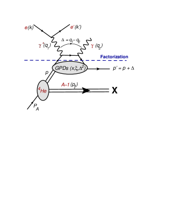
Figure 1: (color online) Incoherent DVCS process off ⁴He in the IA to the handbag approximation.

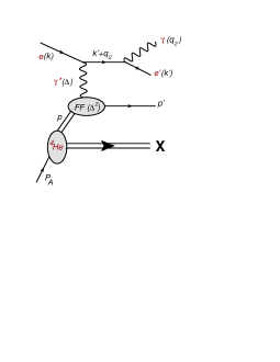
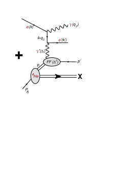
Figure 2: (color online) The Bethe Heitler process in IA.

In our IA approach, we account only for the kinematical off-shellness of the initial bound proton so that the energy of the struck proton is obtained from energy conservation and reads

$$p_{0}=M_{A}-\sqrt{M_{A-1}^{*2}+\vec{p}^{2}}\simeq M-E-T_{rec}\,,$$ (4)

where we define the removal energy $E=M^{*}_{A-1}+M-M_{A}=\epsilon^{*}_{A-1}+|E_{A}|-|E_{A-1}|$ in terms of the binding energy (mass) of ⁴He and of the 3-body system, $E_{A}$ ($M_{A}$) and $E_{A-1}$ ($M_{A-1}^{*}$), respectively, and of the excitation energy of the recoiling system, $\epsilon^{*}_{A-1}$. Finally, $T_{rec}$ is the kinetic energy of the recoiling $3-$body system and $M$ is the proton mass. A straightforward but lengthy analysis, detailed in appendix A, leads to a complicated convolution formula for the cross section, which can be cast in the following form

$$d\sigma_{Inc}^{\pm}=\int_{exp}dE\,d{\vec{p}}\,\frac{p\cdot k}{p_{0}\,|\vec{k}|}P^{{}^{4}He}(\vec{p},E)\,d\sigma^{\pm}_{b}(\vec{p},E,K)\,,$$ (5)

where the main ingredients are the nuclear spectral function $P^{{}^{4}He}(\vec{p},E)$ and the cross section for a DVCS process off a bound proton, $d\sigma^{\pm}_{b}$. As thoroughly described in Appendix A, the integral on the removal energy refers to the full spectrum of ⁴He, both discrete and continuous. In Eq. (5), $K$ is the set of kinematical variables $\{x_{B}=Q^{2}/(2M\nu),Q^{2},t,\phi\}$. The range of $K$ accessed in the experiment fixes the proper energy and momentum integration space, denoted as $exp$ and described in appendix A. From Eq. (5) we get the measured differential cross sections, appearing in Eq. (3),

$$d\sigma^{\pm}\equiv\frac{d\sigma^{\pm}_{Inc}}{d{x}_{B}dQ^{2}d{\Delta}^{2}d\phi} =\int_{exp}dE\,d{\vec{p}}\,P^{{}^{4}He}(\vec{p},E)$$

$$\times|\mathcal{A}^{\pm}({\vec{p}},E,K)|^{2}g(\vec{p},E,K)\,,$$

where $g(\vec{p},E,K)$ is a complicated function which arises, as explicitely detailed in Appendix A, from the integration over the phase space and includes also the flux factor ${p\cdot k}/({p_{0}\,|\vec{k}|})$ of Eq. (5). This latter term comes from the fact that one has at disposal only non-relativistic nuclear wave functions to evaluate the spectral function. In the present approach this implies that the number of particle sum rule is respected, but the momentum sum rule is slightly violated. Such a problem could be solved ultimately within a Light Front approach, along the lines proposed in Ref. DelDotto:2016vkh for a $3-$body system.

The BSA (3), written in terms of the above cross sections, yields the schematic form

$$A_{LU}^{Incoh}(K)=\frac{\mathcal{I}^{{}^{4}He}(K)}{T_{BH}^{2\,\,^{4}He}(K)}\,,$$ (7)

where

$$\mathcal{I}^{{}^{4}He}(K)=\int_{exp}dE\,d\vec{p}\,{{P^{{}^{4}He}(\vec{p},E)}}\,g(\vec{p},E,K)\,{{\mathcal{I}(\vec{p},E,K)}}\,,$$

$$T_{BH}^{2\,\,^{4}He}(K) = \int_{exp}dE\,d\vec{p}\,{{P^{{}^{4}He}(\vec{p},E)}}\,g(\vec{p},E,K)\,$$ (8)

$$\times {{T_{BH}^{2}(\vec{p},E,K)}}\,,$$

refer to a moving bound nucleon and generalize the Fourier decomposition of the DVCS cross section off a proton at rest, at leading twist, derived in Ref. Belitsky:2001ns . Without going into technical details, that are presented in appendix B, we summarize the structure of the different contributions.
For the BH part, we considered the full sum of azimuthal harmonics, i.e

$$T_{BH}^{2}=c_{0}^{bound}+c_{1}^{bound}\cos\phi+c_{2}^{bound}\cos(2\phi)\,,$$ (9)

where the coefficients $c_{i}^{bound}$ contain the Dirac and Pauli form factors (FFs). The azimuthal dependence of the amplitudes is due to the expression of the BH propagator as reported in Appendix B. We stress that in the present IA approach no nuclear modifications occur for the FFs of the bound proton. Concerning the interference part in the numerator of Eq. (3), terms proportional to $\Delta^{2}/Q^{2}$ have been considered as well as corrections proportional to $\epsilon^{2}=4M^{2}x_{B}^{2}/{Q^{2}}$, accounting for target mass corrections. The latter terms are fundamental in order to obtain a fully consistent comparison with the BSA for a proton at rest, which will be shown in the next section. The main reason is that in the amplitudes for a bound proton it is not always possible to isolate such terms, since the obtained expressions are function of the 4-momentum of the bound, off-shell proton. In our approach the parton content of the bound proton plays a role only in the imaginary part of the CFF $\mathcal{H}$. In the kinematics of interest and in the present model, this quantity can be expressed in terms of only one GPD of the bound proton, $H(x,\xi,\Delta^{2})$, selected in the slice $x=\pm\xi$ , i.e.

$$\Im m\mathcal{H}(\xi^{\prime},t)=H(\xi^{\prime},\xi^{\prime},t)-H(-\xi^{\prime},\xi^{\prime},t)\,,$$ (10)

where $H(\xi^{\prime},\xi^{\prime},t)$ is summed over the $u,d,s$ flavours of the quarks. We notice that the off-shellness of the bound nucleon enters the proton parton structure through the dependence of the GPDs on $\xi^{\prime}={-q^{2}}/({P\cdot q})$. In this way, the modification at partonic level is due to this rescaling of the skewness that, for a proton at rest, becomes $\xi=x_{B}(1+\Delta^{2}/2Q^{2})/(2-x_{B}+x_{B}\Delta^{2}/Q^{2})$, keeping terms proportional to $\Delta^{2}/Q^{2}$.

Figure 3: Beam spin asymmetry for a proton at rest considering (full curve) and ignoring (dot-dashed curve) term of order $\Delta^{2}/Q^{2}$ in the interference part. In this kinematics, $\Delta^{2}/Q^{2}\simeq 0.144$. Data from Ref. Girod:2007aa .

Figure 4: The cross section for the BH process on the free proton (dashed line) and on a proton bound in ⁴He (full line), according to the present treatment, in the kinematics reported on the top of the frame, corresponding to data presented in Ref. HirlingerSaylor:2018bnu , as a function of the azimuthal angle $\bm{\phi}$. The precise position of the data and their errors are taken from CLAS .

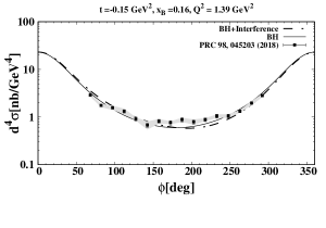
Figure 5: The cross section for the BH process (full line) and the one obtained including the interference between the BH and DVCS processes (dot-dashed line), for a proton bound in ⁴He, according to the present treatment, in the kinematics reported on the top of the frame, corresponding to data presented in Ref. HirlingerSaylor:2018bnu , as a function of the azimuthal angle $\bm{\phi}$. The precise position of the experimental data and their errors are taken from CLAS .

Figure 6: The cross section for the bound proton (full line) and for the free proton (dot-dashed line) in the kinematics reported on the top of the frame, corresponding to data presented in Ref. HirlingerSaylor:2018bnu , as a function of the azimuthal angle $\bm{\phi}$. The precise position of the data and their errors are taken from CLAS .

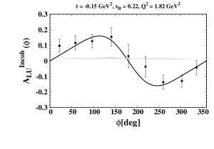
Figure 7: The BSA $A_{LU}^{Incoh}$, Eq. (7), as a function of the azimuthal ange $\bm{\phi}$, compared to data corresponding to the analysis leading to Ref Hattawy:2018liu

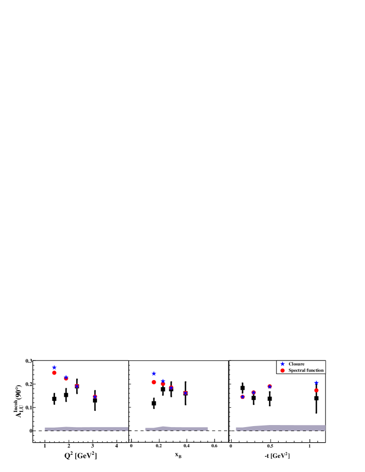
5

Figure 8: (Color online) Azimuthal beam-spin asymmetry for the proton in ⁴He, $A_{LU}^{Incoh}(K)$, for $\phi=90^{o}$: results of this approach (red dots are obtained using the diagonal spectral function as described along the text, blue stars using the momentum distribution in the so called ”closure approximation” ) compared with data (black squares) Hattawy:2017woc . From left to right, the quantity is shown in the experimental $Q^{2}$, $x_{B}$ and $t$ bins, respectively. Shaded areas represent systematic errors.

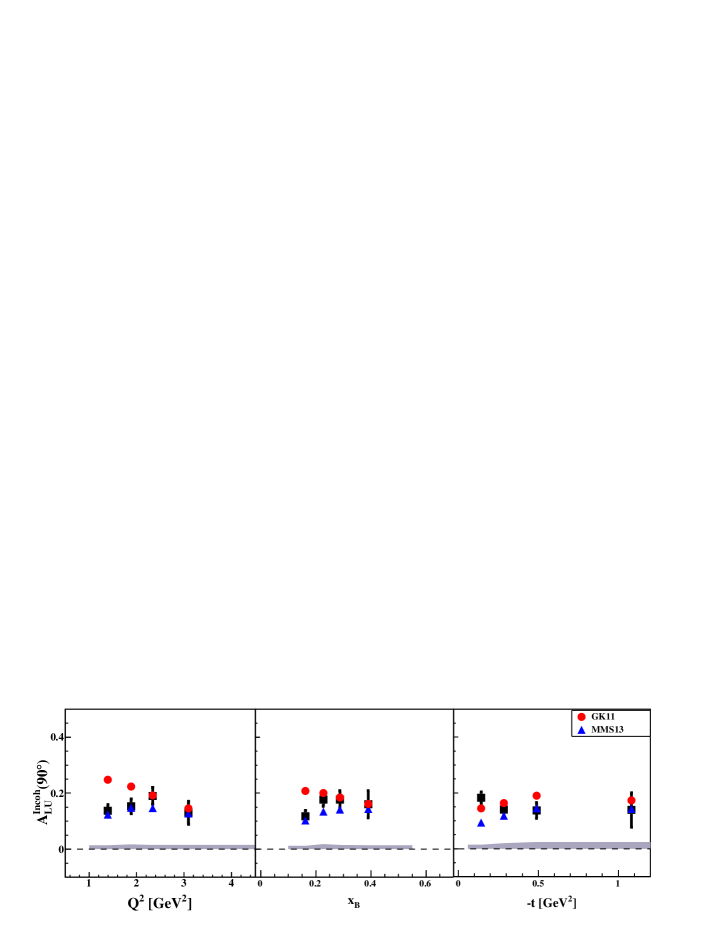
Figure 9: (Color online) Azimuthal beam-spin asymmetry for the proton in ⁴He, $A_{LU}^{Incoh}(K)$, for $\phi=90^{o}$: results of this approach (red dots are obtained using the GK GPD model Goloskokov:2011rd , blue triangles using the MMS model Mezrag:2013mya ) compared with data (black squares) Hattawy:2017woc . From left to right, the quantity is shown in the experimental $Q^{2}$, $x_{B}$ and $t$ bins, respectively. Shaded areas represent systematic errors.

III Ingredients of the calculation

In order to actually evaluate Eq. (7), we need an input for the proton GPD and for the proton spectral function in ⁴He. Concerning the nuclear part, only old attempts exist of obtaining a complete spectral function of ⁴He Morita:1991ka ; trento . The unpolarized spectral function, whose emergence in this process is thoroughly described in appendix A, can be cast in the form

$$P^{{}^{4}He}(\vec{p},E) = \sum_{f_{A-1}}\langle{{}^{4}He}|f_{A-1};N\,\vec{p}\,\rangle\langle f_{A-1};N\,\vec{p}\,|{{}^{4}He}\rangle$$ (11)

$$\times \delta(E-E_{min}-\epsilon_{A-1}^{*})\,.$$

It is therefore clear that its realistic evaluation would require the knowledge, at the same time, of exact solutions of the Schrödinger equation with realistic nucleon-nucleon potentials and three-body forces for the ⁴He nucleus and for the three-body recoiling system $f_{A-1}$. This system can be either in its ground state, when $E=E_{min}=|E_{{}^{4}He}|-|E_{{}^{3}H}|$, or unbound with an excitation energy $\epsilon^{*}_{A-1}$. The description of this latter part represents a challenging few-body problem, whose solution is presently unknown. A full realistic calculation of the ⁴He spectral function is planned and has started but, in this work, for $P^{{}^{4}He}(\vec{p},E)$ use is made of the model presented in Ref. Viviani:2001wu ; Rinat:2004ia . In that approach, when the recoiling system is in its ground state and $E=E_{min}$, an exact description is used in terms of variational wave functions for the 4-body PisaWF and 3-body PisaWF3 systems, obtained through the hyperspherical harmonics method hh , within the Av18 NN interaction Wiringa:1994wb , including UIX three-body forces Pudliner:1995wk . The cumbersome part of the spectral function, with the recoiling system excited, is based on the Av18+UIX interaction, proposed in Ref. Viviani:2001wu ; Rinat:2004ia , an update of the two-nucleon correlation model of Ref. CiofidegliAtti:1995qe . We note that realistic calculations of GPDs for ³He, for which an exact spectral function is available, have established the importance of properly considering the $E$-dependence of the spectral function Scopetta:2009sn . To have an idea of the importance of a proper treatment of the $E$-dependence in this process, and, in general, of the drawback of the use of a less refined nuclear description, in the next section we will show also results obtained using the so called ”closure” approximation. It consists in evaluating the spectral function considering, in the argument of the delta function in Eq. (11), an average value of the removal energy, so that the closure of the $f_{A-1}$ states can be used, yielding

$$P^{{}^{4}He}_{closure}(p,E) = n_{gr}(p)\delta(E-E_{min})$$ (12)

$$+ n_{ex}(p)\delta(E-\bar{E})\,,$$

where the momentum distribution for the proton with the recoiling system in its ground or excited state, $n_{gr}(k)$ and $n_{ex}(k)$, respectively, have been introduced, with $\bar{E}$ the average excitation energy of the recoiling system. A similar approach has been used to model the non-diagonal ⁴He spectral function in the description of coherent DVCS off ⁴He, in Ref. Fucini:2018gso . We note that, when this approximation is used, also the off-shellness of the struck proton, governed by Eq. (12), has to be changed accordingly, i.e.

$$p_{0}=M_{A}-\sqrt{M_{A-1}^{*2}+\vec{p}^{2}}\longrightarrow M-\bar{E}-T_{rec}\,.$$ (13)

As we will see in the following, this produces important effects in the cross section, due to the fact that the components of the four momentum of the proton enter scalar products present in the relevant scattering amplitudes.

For the nucleonic GPD, two models have been used. One is the model of Goloskokov and Kroll (GK) Goloskokov:2011rd , already successfully exploited in the coherent case Fucini:2018gso . It is worth to remind that the model is valid in principle at $Q^{2}$ values larger than those of interest here, in particular at $Q^{2}\geq 4$ GeV². Nonetheless we have checked that the GK model can reasonably describe free proton data collected in similar kinematical ranges, for example the ones in Ref. Girod:2007aa , as it is discussed in the next section (see Fig. 3).

The other model is taken from Ref. Mezrag:2013mya . It is based on an original compact version of the double distribution prescription. It is developed at leading twist and at leading order in $\alpha_{s}$ (of course NLO corrections may be sizable also in the valence region, at moderate energy, see, e.g., the discussion in Ref. Moutarde:2013qs ). With respect to the GK model, only the valence region is modified and the momentum scale evolution is the same. The model is expected to work in the region $-t/Q^{2}\leq 0.1$, where factorization is supposed to work. To obtain the relevant numbers for that model, use has been made of the virtual access infrastructure ”3DPARTONS” Berthou:2015oaw .

IV Numerical results

We can now evaluate the beam spin symmetry (BSA), Eq. (7) , and compare it with the recently published data Hattawy:2018liu .

First of all, let us check if the GK model we used, for values of $Q^{2}$ smaller than those for which it is supposed to work, $Q^{2}\geq 4$ GeV², is still describing the available data reasonably well. To this aim, we show in Fig. 3 that, in one of the kinematics presented in Ref. Girod:2007aa for DVCS off the free proton, not far from the ones of interest here, a reasonable description of the BSA data, is obtained calculating this quantity for the free proton with the GK model. We notice that the azimuthal angle $\bm{\phi}$, used by the experimental collaboration and exploited here, is related to the one previously defined and used in this paper by the relation $\bm{\phi}=\pi-\phi$. The relevance of terms of order $t/Q^{2}$, discussed in the previous section, is also shown. In general, the BSA is rather sensitive to changes of the kinematics, to $t$ especially. Data for the free proton are not available for the kinematics of the experiment under scrutiny so that we have to compare with results of other experiments.

Then, let us show the results of our model for the differential cross sections (II) which are used later to calculate the BSA. All the cross sections shown here below are obtained considering a positive electron helicity, as an example.

To have a first glimpse at the nuclear effects on the relevant processes, the cross section for the BH process on the free proton (dashed) and on a proton bound in ⁴He (full), according to the present treatment, is shown in Fig. 4, as a function of the azimuthal angle $\bm{\phi}$, in one of the kinematical ranges of the data presented in Ref. HirlingerSaylor:2018bnu . The data, corresponding to the full DVCS process off the free proton, are presented here for illustration only. Relevant nuclear effects are clearly seen. To our knowledge, this figure and the next two are the first ones in the literature where the comparison of cross sections for free and bound nucleons, with a difference arising from a microscopic calculation, is presented.

In Fig. 5, the cross section for the BH process is compared with that obtained including also the only relevant term, as discussed in Appendix B, of the the interference between the BH and DVCS processes, for a proton bound in ⁴He according to the present treatment, again in the kinematics of Ref. HirlingerSaylor:2018bnu , as a function of the azimuthal angle $\bm{\phi}$ (see Appendix B for the discussion of the relevant term included). It is clearly seen as a relevant $\phi$ asymmetry is generated including the DVCS mechanism. The data for the free proton are again reported for illustration. It is seen that a reasonable description is obtained.

In Fig. 6, in the same kinematics of the previous two, the full cross section is shown, for a bound and for a free proton, to expose the role of the nuclear effects on the proton DVCS cross-section, found to be overall sizable.

Let us now present results for the BSA $A_{LU}^{Incoh}$, Eq. (7). This quantity, evaluated using the GK model for the GPD entering the DVCS part, is shown in Fig. 7, as a function of the azimuthal ange $\bm{\phi}$, compared to data corresponding to the analysis leading to Ref Hattawy:2018liu . A convincing agreement is found, in particular at $\bm{\phi}=\phi=90^{o}$, the fixed value at which the BSA has been extracted and at which it will be shown in the following.

The BSA is a function of the azimuthal angle $\phi$ and of the kinematical variables $Q^{2}$, $x_{B}$ and $t$. Due to limited statistics, in the experimental analysis these latter variables have been studied separately with a two-dimensional data binning. The same procedure has been used in our calculation. For example, each point at a given $x_{B}$ has been obtained using for $t$ and $Q^{2}$ the corresponding average experimental values, which are reported for definiteness in Tables I-III, together with the numerical values of the calculated theoretical asymmetries discussed in the following.

$x_{B}$	$<Q^{2}>$ [GeV2]	$<t>$ [GeV2]	$A_{LU}^{GK}$	$A_{LU}^{MMS}$
0.162	1.43	-0.397	0.208	0.102
0.227	1.92	-0.418	0.204	0.134
0.287	2.35	-0.492	0.185	0.141
0.390	2.98	-0.714	0.163	0.143

Table 1: The BSA, obtained using the GK Goloskokov:2011rd or MMS Mezrag:2013mya models, using the nuclear spectral function, for the average values of $Q^{2}$ and $t$ in $x_{B}$ bins.

$Q^{2}$ [GeV2]	$<x_{B}>$	$<t>$ [GeV2]	$A_{LU}^{GK}$	$A_{LU}^{MMS}$
1.40	0.166	-0.407	0.248	0.124
1.89	0.233	-0.499	0.224	0.148
2.34	0.290	-0.521	0.192	0.147
3.10	0.379	-0.650	0.146	0.128

Table 2: The BSA, obtained using the GK Goloskokov:2011rd or MMS Mezrag:2013mya models, using the nuclear spectral function, for the average values of $x_{B}$ and $t$ in $Q^{2}$ bins.

$t$ [GeV2]	$<x_{B}>$	$<Q^{2}>$ [GeV2]	$A_{LU}^{GK}$	$A_{LU}^{MMS}$
-0.145	0.213	1.82	0.145	0.094
-0.282	0.255	2.13	0.164	0.118
-0.490	0.284	2.31	0.190	0.144
-1.11	0.308	2.41	0.173	0.140

Table 3: The BSA, obtained using the GK Goloskokov:2011rd or MMS Mezrag:2013mya models, using the nuclear spectral function, for the average values of $x_{B}$ and $Q^{2}$ in $t$ bins.

In Fig. 8 it is seen that, overall, the calculation reproduces the data rather well in all of these bins. For this observable, in most of the cases the present accuracy of the data does not allow to distinguish between the full calculation and that performed using the closure approximation, Eq. (12). In any case, whenever the disagreement with the data is sizable, the proper treatment of the excitation energy within the spectral function helps in describing the data. Besides, we note that the agreement is not satisfactory only when the GK model is used in the region of low $Q^{2}$. Indeed, this is evident only in the experimental points corresponding to the lowest values of $Q^{2}$, $x_{B}$ and $t$. One should notice that the average value of $Q^{2}$ grows with increasing $x_{B}$ and $t$ (cf. tables I-III), so that a not satisfactory description at low $Q^{2}$ affects also the first $x_{B}$ and $t$ bins. Actually, the GK model is designed to describe the available data for $Q^{2}\leq 4$ GeV², e.g at values higher than the typical ones accessed by the CLAS collaboration in the experiment under scrutiny. The problems found using the GK parametrization are therefore somehow expected. We have therefore repeated the calculation using as a nucleonic partonic input the model MMS, introduced in Ref. Mezrag:2013mya , briefly described in the previous section. The comparison of the two results is presented in Fig 9, where it is seen that the data favor the MMS model with respect to the GK one. The success of the MMS model, with parameters chosen precisely to be realistic in the $Q^{2}$ range typical at JLab, is remarkable and points to a solid predictivity of the IA, emphasizing, at the same time, the dependence of the results on the choice of the nucleonic model. In any case, the residual disagreement, or the problems found using the GK model, could be also due to some final state interaction (FSI) effects that in the present IA are not considered. For this reason, a careful analysis of the interplay between the $t$ and $Q^{2}$ dependence of the data is required to establish whether FSI play a relevant role. The present accuracy of the data does not allow such an analysis, but the data expected from the planned future measurements certainly will. In the light of this discussion, we can conclude that a careful use of basic conventional ingredients is able to reproduce the available data. In order to better understand our results, addressing nuclear modifications of the parton strucure, possibly related therefore to the EMC effect, as an illustration we perform a specific analysis, detailed in what follows.

Let us define, in each experimental bin, specific ratios to expose the nature of nuclear effects, namely, the ratio between the BH-DVCS interference cross section for the proton bound in ⁴He and the free one at rest, $R_{\mathcal{I}}(K)$, the corresponding quantity for the pure $BH$ process, $R_{{BH}}(K)$, and the ratio of the two, $R_{ALU}(k)$, providing the ratio of the bound proton to the free proton $BSA$ in our calculation scheme. These quantities read, respectively

$$R_{\mathcal{I}}(K) = \frac{1}{\mathcal{N}}\frac{{I}^{{}^{4}He}(K)}{{I}^{p}(K)}\,,$$ (14)

$$R_{BH}(K) = \frac{1}{\mathcal{N}}\frac{T_{BH}^{2\,\,^{4}He}(K)}{T_{BH}^{2\,p}(K)}\,,$$ (15)

$$R_{ALU}(K) = \frac{R_{\mathcal{I}}(K)}{R_{BH}(K)}=\frac{A_{LU}^{Incoh}(K)}{A_{LU}^{p}(K)}\,.$$ (16)

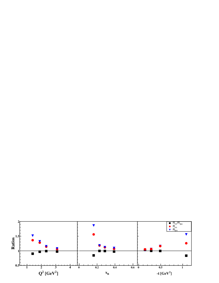
Figure 10: (Color online) The ratios (14) (red dots), (15) (blue triangles), (16) (black squares), at $\phi=90^{o}$ and using the GK model for the nucleon GPD. From left to right, the quantity is shown in the experimental $Q^{2}$, $x_{B}$ and $t$ bins, respectively.

In the equations above the factor ${\cal N}=\int_{exp}dE\,d\vec{p}P^{{}^{4}He}(\vec{p},E)$ accounts for the fact that only a part of the spectral function is selected in a given experimental bin. The meaning of the integration space $exp$ is clarified in appendix $A$. The ratios (14)-(16) at $\phi=90^{o}$, using the GK model for the nucleon GPD, are shown in Fig. 10. It is clearly seen that the nuclear effects obtained within the present IA scheme in the ratios (14) and (15) are rather sizable, while the effects are dramatically reduced in the ”super-ratio” (16). This fact points to relevant conventional nuclear effects in the pure BH and pure DVCS processes, which are anyhow of a similar origin, so that they cancel out to a large extent in the ratio.

Something similar happens when the closure approximation is applied to estimate the nuclear effects. In Figs. 11 and 12 it is seen that, in some cases, the difference between the results of the full calculation, performed considering the distribution of the removal energy within the spectral function, and of the one obtained with the closure approximation, is rather sizable in the ratio (14) and (16). In Fig. 14 is seen instead that the effect is dramatically reduced in the ratio of these two quantities, the super-ratio (16), showing that the effects in the numerator and in the denominator basically compensate each other.

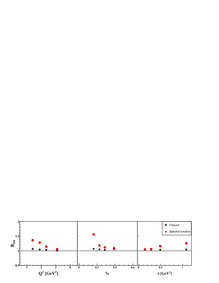
Figure 11: (Color online) The ratio (14) (blue triangles), obtained using either the spectral function (red dots) or the closure approximation (black stars), at $\phi=90^{o}$ and using the GK model for the nucleon GPD. From left to right, the quantity is shown in the experimental $Q^{2}$, $x_{B}$ and $t$ bins, respectively.

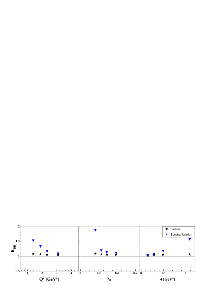
Figure 12: (Color online) The ratio (15), evaluated using the spectral function (blue triangles) and the closure approximation (black stars) for $\phi=90^{o}$ and using the GK model for the proton GPD. From left to right, the quantity is shown in the experimental $Q^{2}$, $x_{B}$ and $t$ bins, respectively.

Figure 13: (Color online) The ratio (16), evaluated using the spectral function (blue triangles) and the closure approximation (black stars) for $\phi=90^{o}$ and using the GK model for the proton GPD. From left to right, the quantity is shown in the experimental $Q^{2}$, $x_{B}$ and $t$ bins, respectively. The results is compared with the same ratio estimated by the EG6 collaboration (black squares). clastobe .

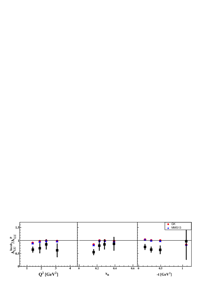
Figure 14: (Color online) The ratio (16) of the azimuthal beam-spin asymmetry for the proton in ⁴He, $A_{LU}^{Inco,h}(K)$, to the corresponding quantity for the free proton at rest, for $\phi=90^{o}$, using for the proton GPD the GK model Goloskokov:2011rd (red dots), and the MMS model Mezrag:2013mya (blue triangles) compared with the ratio estimated by the EG6 collaboration (black squares) clastobe . From left to right, the quantity is shown in the experimental $Q^{2}$, $x_{B}$ and $t$ bins, respectively.

The dots shown in this latter figure are related to another intriguing observation, obtained following a procedure used by the experimental collaboration to expose nuclear effects Hattawy:2018liu . Our BSA for the proton bound in ⁴He has been divided by the corresponding quantity for a free proton at rest, using the GK model, and plotted as a function of $x_{B}$. It is seen that the results underestimate those obtained in the analysis of the experimental collaboration. This points to interesting effects not included in the present IA scheme, either at the parton level (medium modifications of the parton structure due exotic effects, such as dynamical off-shellness) or of conventional origin, such as FSI, not yet included in the calculation. In Fig. 14 we show the results obtained with the spectral function and with either the GK or the MMS model, almost indistinguishable between themselves. Clearly, while in the result for $A_{LU}$ the difference between the different models was in some cases sizable, in this specific quantity, which can be built in principle from data taken for protons in ⁴He and for the free proton at the same kinematics, this ratio seems to be be essentially independent on the model used for the nucleon. In general nuclear effects are found to be rather small in IA for this quantity, which seems therefore very promising to expose exotic nuclear effects.

To dig further into this interesting result and to realize to what extent a medium modification of the parton structure is predicted by our calculation, we observe that the ratio (16) can be sketched as follows

$$\frac{A_{LU}^{Incoh}}{A_{LU}^{p}}=\frac{\mathcal{I}^{{}^{4}He}}{\mathcal{I}^{\,p}}\frac{T_{BH}^{2\,\,p}}{T_{BH}^{2\,\,^{4}He}}\propto\frac{(nucl.eff.)_{\mathcal{I}}}{(nucl.eff.)_{BH}}\,,$$ (17)

i.e., it is proportional to the ratio of the nuclear effects on the BH-DVCS interference to the nuclear effects on the pure BH cross section. If the nuclear dynamics modifies $\mathcal{I}$ and the $T_{BH}^{2}$ in a different way, the effect can be big even if the parton structure of the bound proton does not change appreciably. We analyze this occurrence in Fig. 15, where, together with the ratio (16), we show two others quantities, as functions of $x_{B}$. One of them, labelled ”pointlike”, is obtained considering in the ratio pointlike protons. It is seen that, at low $x_{B}$, where sizable effects are found within our IA approach, the big effect is still there. Besides, in the same figure we show an ”EMC-like” quantity, i.e., a ratio of a nuclear parton observable, the imaginary part of the CFF, to the $same$ observable for the free proton:

$$R_{EMC-like}=\frac{1}{{\cal N}}\frac{\int_{exp}dE\,d\vec{p}\,P^{{}^{4}He}(\vec{p},E)\,\Im m\,\mathcal{H}(\xi^{\prime},\Delta^{2})}{\Im m\,\mathcal{H}(\xi,\Delta^{2})}\,.$$ (18)

One should notice that this ratio would be one if nuclear effects $in$ $the$ $parton$ $structure$ were negligible. As seen in Fig. 15, this ratio is close to one and it resembles the EMC ratio, for ⁴He, at low $x_{B}$ (cf the data in Ref. Seely:2009gt ). Since in our analysis the inner structure of the bound proton is entirely contained in the CFF and this produces a mild modification, the sizable effect found for the ratio (17) for the first $x_{B}$ bin, shown in Fig. 15, has little to do with the modifications of the parton content driven by the IA and analyzed here. Rather, the effect is due to a different dependence on the 4-momentum components, affected by nuclear effects, of the interference and BH terms for the bound proton.

It will be very interesting to study the ratio (16) when consistently collected data will be available for the proton and for ⁴He, to look for effects to be ascribed to exotic modifications of the parton content or to a complicated conventional behaviour, beyond IA.

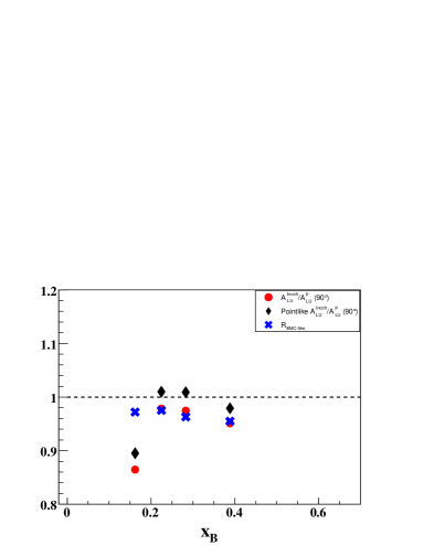
Figure 15: (color online) The ratio $A_{LU}^{Incoh}/{A_{LU}^{p}}$, Eq. (17) (red dots), compared to the result obtained with pointlike protons (black diamonds) and to the EMC-like ratio Eq. (18) (blue crosses).

V Conclusions

An impulse approximation analysis, based on state-of-the-art models for the proton and nuclear structure, using a conventional description in terms of nucleon degrees of freedom, has been thoroughly described. Recent data on incoherent DVCS off ⁴He are overall well reproduced.

The results can be summarized as follows:

i) the main experimental observable, the only one measured so far, the BSA, turns out to be sensitive to the nucleonic model used, in particular at low values of $Q^{2}$; parametrizations for generalized parton distributions based on high $Q^{2}$ data seem to have limited predictive power in the low $Q^{2}$ sector;

ii) given the present accuracy of the data, the beam spin asymmetry is mildly sensitive to the details of the nuclear model used in the calculation, as it can be argued using a spectral function or its closure approximation. Results obtained within the spectral function are anyway closer to a good description of the data;

iii) the behaviour at low $Q^{2}$ could point also to possible FSI effects, to be investigated, or to other quark and gluon effects. The present accuracy of the data does not allow a further analysis towards this direction;

iv) a careful study of nuclear effects in the different processes contributing to the BSA, the BH in the denominator and the DVCS-BH-Interference in the numerator, has exposed sizable effects; besides, a clear difference is found, in some kinematical points, if the spectral function or the closure approximation are used. The separated measurements of these contributions, which correspond to those of the differential cross sections and not only to their ratio, would be very interesting and deserve to be attempted in the future experiments;

v) all these effetcs actually basically disappear in the ratio of the interference to the BH contributions. In our IA approach, the latter ratio represents that between the BSA for incoherent DVCS off ⁴He and coherent DVCS off the free proton. Its stability against different nuclear and nucleon models, found in this study, demonstrates that it can be used to expose interesting exotic effects beyond the ones included in IA. We can preliminarly assert that our calculation of this quantity overestimates the estimate of the experimental collaboration.

We would conlcude that, given the present accuracy of the data, there is no point in going beyond the exhaustive analysis presented here. New tagged measurements with detection of residual nuclear final states, planned at JLab Armstrong:2017zcm and under study for the future EIC, will shed more light to this respect. The presence of specific nuclear final states in these processes will also make possible a precise evaluation of FSI in terms of few-body realistic wave functions, allowing for a conclusive comparison with data.

While a benchmark calculation in the kinematics of the next generation of precise measurements will require an improved treatment of both the nucleonic and the nuclear parts of the calculation, such as a realistic evaluation of the diagonal spectral function of ⁴He, the straightforward approach proposed here can be used as a workable framework for the planning of future measurements. Possible exotic quark and gluon effects in nuclei, not clearly seen within the present experimental accuracy, will be exposed by comparing forthcoming data with our conventional results. To this aim, a novel Montecarlo event generator topeg , tested so far with our model of the coherent process, will be used to simulate incoherent DVCS off ⁴He, described within the approach presented here, to plan the next generation of experiments at JLab and at the future EIC.

Appendix A The convolution formula

Let us start considering the cross section $d\sigma^{\pm}$ appearing in Eq. (3). It can be written in a generic frame, for the incoherent channel of the DVCS process under scrutiny, namely $e(k)A(P_{A})\rightarrow e(k^{\prime})N(p_{N})\gamma(q_{2})X(p_{X})$ off a nuclear target $A$, in the following way

$$(d\sigma^{\pm})_{Inc}=(2\pi)^{4}\frac{1}{4P_{A}\cdot k}\sum_{\sigma}\sum_{N}\sum_{X}|{\mathcal{A}}^{\pm}|^{2}\delta({P}_{A}+{k}-{k}^{\prime}-{p}_{X}-{p}_{N}-{q}_{2})d{\tilde{p}}_{X}d{\tilde{k}}^{\prime}d{\tilde{q}}_{2}d{\tilde{p}}_{N}$$ (19)

where the dynamical information is encoded in the squared amplitude. The latter is given by three different contributions, namely $|{\mathcal{A}}|^{2}=|{\mathcal{A}}_{DVCS}|^{2}+|{\mathcal{A}}_{BH}|^{2}+\mathcal{I}_{BH-DVCS}$. A generic phase-space integration volume reads

$$d{\tilde{k}}\equiv\frac{d^{3}k}{(2\pi)^{3}2k_{0}}.$$ (20)

In Eq. (19), the sums are extended to the inner nucleons of type $N$ in the target, to the polarization $\sigma$ of the final detected proton and to the undetected nuclear system $X$. The status $f$ of the latter is identified by a set $\{\alpha_{f}\}$ of discrete quantum numbers and by the excitation energy $E_{f}$, for which discrete and continuous values are possible. One has therefore, in Eq. (19),

$$\sum_{X}d{\tilde{p}}_{X}\rightarrow\sum_{f}\displaystyle\sum_{\{\alpha\}_{f}}\sumint_{E_{f}}\rho(E_{f})\,d{\tilde{p}}_{f}\,,$$ (21)

where $\rho(E_{f})$ is the density of final states. The amplitudes $\mathcal{A}_{BH}$ and $\mathcal{A}_{DVCS}$ appearing in Eq.(19) are given by the contraction of a leptonic tensor ($L^{\nu}_{DVCS}/Q^{2}$ and $L^{\mu\nu}_{BH}/\Delta^{2}$ for $DVCS$ and $BH$, respectively) with the appropriate hadronic tensor. For a generic DVCS process of a target $A$ with initial(final) polarization $S(S^{\prime})$ reads

$$T_{\mu\nu}^{DVCS}(P_{A},\Delta,q,S,S^{\prime})=\int dre^{iq\cdot r}\langle P^{\prime}_{A}S^{\prime}|T\{\hat{J}_{\mu}(r)\hat{J}_{\nu}(0)\}|P_{A}S\rangle\,.$$ (22)

Since a convolution formula with the same structure can be obtained for any of the $DVCS$, $BH$ and interference terms exploiting the same steps, to fix the ideas in what follows we specify our treatment to the $DVCS$ part. Let us consider therefore the scattering amplitude of the incoherent DVCS process off an ⁴He target, i.e $e(k)^{4}He(P_{A})\rightarrow e(k^{\prime})N(p_{N})\gamma(q_{2})X(p_{X})$

$${\mathcal{A}}_{DVCS}^{A,N,f}=-ie\sum_{\lambda^{\prime}}\bar{u}(k^{\prime},\lambda^{\prime})\gamma_{\mu}u(k,\lambda)\frac{1}{Q^{2}}T_{A,N,f}^{\mu\nu}\epsilon_{\nu}^{*}(q_{2})=\frac{\epsilon_{\nu}^{*}(q_{2})}{Q^{2}}L_{\mu}^{DVCS}(\lambda)T_{A,N,f}^{\mu\nu}\,,$$ (23)

where it appears the hadronic tensor $T^{A,N}_{\mu\nu}$, defined in terms of

$$T^{A,N}_{\mu\nu}=\int d^{4}re^{-iq\cdot r}H_{\mu\nu}^{A,N}\,,$$ (24)

being $H_{\mu\nu}^{A,N}$ the matrix element of $\hat{O}^{N}=T\{\hat{J}^{N}_{\mu}(x)\hat{J}^{N}_{\nu}(0)\}$ properly evaluated between the states describing the initial and the final nucleon $N$ in the nucleus $A$, respectively. Here and in the following, we are assuming that the interaction goes through the nucleons in the nucleus, which are the only degrees of freedom in the present Impulse Approximation (IA). Disregarding for the moment the integration on $x$, let us focus on the matrix element $H_{\mu\nu}^{A,N,f}$.
We will use in the following the standard covariant normalization of the states

$$\langle{p}\sigma|{p}^{\prime}\sigma^{\prime}\rangle=(2\pi)^{3}2p_{0}\delta(\vec{p}^{\prime}-\vec{p})\delta_{\sigma,\sigma^{\prime}}$$ (25)

and the notation $\sum_{{p}}=\int d\tilde{p}$ is used. The matrix element in Eq. (24) is therefore

$$H^{A,N,f}_{\mu\nu}=\langle{p}_{N}\sigma,\,{p}_{f}{\{\alpha_{f}\}}E_{f}|\hat{O}_{N}|{P}_{A}\rangle\,,$$ (26)

where the final state contains the detected nucleon with momentum $p_{N}$ and polarization $\sigma$ and the $A-1$- body system described by a set of quantum numbers $\{\alpha_{f}\}$, whose constituents are moving with momenta $p_{f}$. Let us insert to the left and to the right-hand sides of the hadronic operator two complete sets of states; the first set corresponds to the nucleon $N$, supposed free, interacting with the virtual photon, whose completeness reads

$$\sum_{{p}^{\prime}_{N}\sigma^{\prime}}|{p}^{\prime}_{N}\sigma^{\prime}\rangle\langle{p}^{\prime}_{N}\sigma^{\prime}|=1,$$ (27)

while the completeness of the second set of states, describing the hadronic undetected system, is given by:

$$\sum_{\{\alpha_{f}\}}\sumint_{E_{f}}\rho(E_{f})\sum_{{p}_{f}}|{{p}_{f}}\{\alpha_{f}\}{E_{f}}\rangle\langle{{p}_{f}}\{\alpha_{f}\}{E_{f}}|=1~{}.$$ (28)

Now let us use the IA. This means that the interaction goes only through the nucleons, as already said, and that the final state can be written as a tensor product

$$|{p}_{N}\sigma,{p}_{f}\{\alpha_{f}\}E_{f}\rangle=|{p}_{N}\sigma\rangle\otimes|{p}_{f}\{\alpha_{f}\}E_{f}\rangle,$$ (29)

i.e., the interactions between the particles in the final state (FSI) have been neglected. At the light of these facts, we arrive to the following formula

$$H^{A,N,f}_{\mu\nu} = \sum_{\{\alpha^{\prime}_{f}\}}\sumint_{E^{\prime}_{f}}\rho(E^{\prime}_{f})\sum_{{p^{\prime}}_{f}}\sum_{{p}^{\prime}_{N}\sigma^{\prime}}\langle{p}_{N}\,\sigma|\langle{p}_{f}\{{\alpha_{f}}\}E_{f}|\hat{O}_{N}|{p^{\prime}}_{f}\{\alpha_{f}^{\prime}\}E_{f}^{\prime}\rangle|{p^{\prime}}_{N}\sigma^{\prime}\rangle\langle{p^{\prime}}_{N}\sigma^{\prime}|\langle{p^{\prime}}_{f}\{\alpha^{\prime}_{f}\}E_{f}^{\prime}|{P}_{A}\rangle.$$ (30)

Now, assuming in IA that the one-body operator $\hat{O}_{N}$ acts only on the nucleonic states, we can consider the normalization (25) to perform trivially some integrals, obtaining the following form:

$$H^{A,N}_{\mu\nu} = \sum_{{p}_{N}^{{}^{\prime}}\sigma^{\prime}}\langle{p}_{N}\sigma|\hat{O}_{N}|{p}_{N}^{\prime}\sigma^{\prime}\rangle\langle{p}_{f}\{\alpha_{f}\}E_{f}|\langle{p}_{N}^{\prime}\sigma^{\prime}|{P}_{A}\rangle.$$ (31)

A relevant issue has to be discussed at this point. Since relativistic nuclear wave functions for three and four body systems are not at hand, in the following we will be forced to use non relativistic wave functions in the overlaps of the above equation. Therefore, we will use for the states in the overlap a non relativistic normalization

$$\langle\vec{p}s|\vec{p}^{\prime}s^{\prime}\rangle=\delta(\vec{p}-\vec{p}^{\prime})\delta_{ss^{\prime}}\,.$$ (32)

For the same reason, in the overlap we can disentangle the global motion from the intrinsic one

$$|{p}_{f}\{\alpha_{f}\}E_{f}\rangle=|\Phi^{\{\alpha_{f}\}}_{E_{f}}({p}_{f^{\prime}},\sigma_{f^{\prime}});\,{p}_{x}s_{x}\rangle\,,$$ (33)

where $\Phi^{\{\alpha_{f}\}}_{E_{f}}$ represents the intrinsic motion of the final system, described by $A-1$ fully interacting particles, with $A-2$ independent momenta ${p}_{f^{\prime}}$ and intrinsic quantum numbers $\sigma_{f^{\prime}}$, while ${p}_{x}$ and $s_{x}$ specify the state of the center of mass of the $A-1$-body system (for an easy notation, in the following, we will denote the intrinsic wave function simply with the ket $|\Phi^{\{\alpha_{f}\}}_{E_{f}}\rangle$ instead of $|\Phi^{\{\alpha_{f}\}}_{E_{f}}({p}_{f^{\prime}},\sigma_{f^{\prime}})\rangle$). In this way the overlap becomes

$$\{\langle\Phi^{\{\alpha_{f}\}}_{E_{f}}\,{p}_{x}\,s_{x}|\}\langle\vec{p}_{N}\,^{\prime}\sigma^{\prime}|\vec{P}_{A}\rangle=[(2\pi)^{3/2}]^{4}\sqrt{2M_{A}}\sqrt{2p^{\prime 0}_{N}}\sqrt{2p_{x}^{0}}\sqrt{2p_{f}^{0}}\langle\vec{p}_{N}^{\prime}\sigma^{\prime},\Phi^{\{\alpha_{f}\}}_{E_{f}}|{\Phi}_{A}\rangle\,\delta(\vec{P}_{A}-\vec{p}_{x}-\vec{p}_{N}^{\prime})\delta_{\sigma^{\prime},\,-\sigma_{f}-s_{x}}\,,$$ (34)

where the momentum delta function accounts for the center of mass free motion and $\Phi_{A}$ is the intrinsic wave function of the target nucleus. The other delta function yields a formal condition to be fulfilled between the discrete quantum numbers appearing in the overlap. The terms at the beginning of the r.h.s. account for the chosen non relativistic normalization of the states Eq. (32). In this way, from Eq. (31) we get

$$H_{\mu\nu}^{A,N,f} = \sum_{\sigma^{\prime}}\sum_{{p}_{N}^{\prime}}[(2\pi)^{3/2}]^{4}\sqrt{2M_{A}}\sqrt{2p^{\prime 0}_{N}}\sqrt{2p_{x}^{0}}\sqrt{2p_{f}^{0}}\langle{p}_{N}\,\sigma|\hat{O}_{N}|{p}_{N}^{\prime}\sigma^{\prime}\rangle\langle\vec{p}_{N}^{\prime}\sigma^{\prime},\Phi^{\{\alpha_{f}\}}_{E_{f}}|{\Phi}_{A}\rangle\,\delta(\vec{P}_{A}-\vec{p}_{x}-\vec{p}_{N}^{\prime})\delta_{\sigma^{\prime},\,-\sigma_{f}-s_{x}}\,,$$

so that the complete expression for the hadronic tensor in the incoherent DVCS channel becomes:

$$T^{A,N}_{\mu\nu} = \sum_{\sigma^{\prime}}\sum_{{p}_{N}^{\prime}}\int dre^{iq\cdot r}[(2\pi)^{3/2}]^{4}\sqrt{2M_{A}}\sqrt{2p^{\prime 0}_{N}}\sqrt{2p_{x}^{0}}\sqrt{2p_{f}^{0}}\langle{p}_{N}\,\sigma|\hat{O}_{N}|{p}_{N}^{\prime}\sigma^{\prime}\rangle\langle\vec{p}_{N}^{\prime}\sigma^{\prime},\Phi^{\{\alpha_{f}\}}_{E_{f}}|{\Phi}_{A}\rangle\,\delta(\vec{P}_{A}-\vec{p}_{x}-\vec{p}_{N}^{\prime})\delta_{\sigma^{\prime},\,-\sigma_{f}-s_{x}}\,,$$

which can be inserted in the DVCS amplitude Eq. (23) obtaining

$${\mathcal{A}}^{A,N,f,\lambda}_{DVCS} = -ie\sum_{\lambda^{\prime}}\frac{\bar{u}(k^{\prime},\lambda^{\prime})\gamma_{\mu}u(k,\lambda)}{Q^{2}}\sum_{\sigma^{\prime}}\int dre^{iq\cdot r}\sum_{{p}^{\prime}_{N}}\langle{p}_{N}\,\sigma|T({\hat{J}_{N}^{\mu}(r)\hat{J}_{N}^{\nu}(0)})|{p}_{N}^{\prime}\sigma^{\prime}\rangle$$

$$\times [(2\pi)^{3/2}]^{4}\sqrt{2M_{A}}\sqrt{2p^{\prime 0}_{N}}\sqrt{2p_{x}^{0}}\sqrt{2p_{f}^{0}}\langle{p}_{N}\,\sigma|\hat{O}_{N}|{p}_{N}^{\prime}\sigma^{\prime}\rangle\langle\vec{p}_{N}^{\prime}\sigma^{\prime},\Phi^{\{\alpha_{f}\}}_{E_{f}}|{\Phi}_{A}\rangle\,\delta(\vec{P}_{A}-\vec{p}_{x}-\vec{p}_{N}^{\prime})\delta_{\sigma^{\prime},\,-\sigma_{f}-s_{x}}\epsilon^{*}_{\nu}\,.$$

Now, let us consider the squared amplitude appearing in the expression of the cross section, Eq. (19)

$$|{\mathcal{A}}^{A,N,f,\lambda}_{DVCS}|^{2} = (2\pi)^{12}2M_{A}\sum_{\sigma^{\prime\prime}}\sum_{\sigma^{\prime}}\sum_{{p}_{N}^{\prime}}\sum_{{p}_{N}^{\prime\prime}}2p_{x}^{0}2p_{f}^{0}\sqrt{2p_{N}^{\prime 0}}\sqrt{2p_{N}^{{}^{\prime\prime}0}}\bigg{|}\mathcal{A}_{DVCS}^{N,\lambda}({p}_{N},{p}^{\prime}_{N},\sigma,\sigma^{\prime})\bigg{|}^{2}\langle\vec{p}_{N}^{\prime}\sigma^{\prime},\Phi^{\{\alpha_{f}\}}_{E_{f}}|\,{\Phi}_{A}\rangle$$

$$\times \langle{\Phi}_{A}|\,\vec{p}_{N}^{\prime\prime}\sigma^{\prime\prime},\Phi^{\{\alpha_{f}\}}_{E_{f}}\rangle\delta({{\vec{P}}}_{A}-\vec{p}_{x}-{\vec{p}}_{N}^{\prime})\delta({{\vec{P}}}_{A}-{\vec{p}}_{x}-{\vec{p}}_{N}^{\prime\prime})\delta_{\sigma^{\prime},\,(-\sigma_{f}-s_{x})}\delta_{\sigma^{\prime\prime},\,(-\sigma_{f}-s_{x})}\,,$$

where the squared DVCS amplitude off a nucleon is given by

$$|{\mathcal{A}}_{DVCS}^{N\,\lambda}({p}_{N},{p}_{N}^{\prime},\sigma^{\prime})|^{2} = \sum_{\sigma}|{\mathcal{A}}_{DVCS}^{N\,\lambda}({p}_{N},{p}_{N}^{\prime},\sigma,\sigma^{\prime})|^{2}$$

$$= -\frac{g^{\mu\nu}}{Q^{4}}\sum_{\sigma}\int dr^{\prime}e^{-iq\cdot r^{\prime}}\int dre^{iq\cdot r}L_{DVCS}^{\rho}(\lambda)L_{DVCS}(\lambda)^{\sigma\dagger}\langle{p}_{N}\sigma|\hat{O}^{N}_{\mu\nu}|{p}^{\prime}_{N}\sigma^{\prime}\rangle\langle{p}_{N}^{\prime}\sigma^{\prime}|\hat{O}^{N\dagger}_{\rho\sigma}|{p}_{N}\sigma\rangle\,.$$

In this way, substituting the obtained expression in the cross section (19), taking into account that, due to the separation of the global motion from the intrinsic one in the $A-1$ system the sum (21) reads:

$$\sum_{X}d{p}_{X}\rightarrow\sum_{x}\sum_{f^{\prime}}\displaystyle\sum_{\{\alpha\}_{f}}\sumint_{E_{f}}\rho(E_{f})d{\tilde{p}}_{x}d{\tilde{p}}_{f^{\prime}}\,,$$ (38)

and using the delta functions we arrive to

$$(d\sigma^{A})_{Inc} = (2\pi)^{4}\frac{1}{4P_{A}\cdot k}\sum_{N}\sum_{\sigma^{\prime}}\sum_{x}\sum_{f^{\prime}}d\vec{p}_{x}d\vec{p}_{f^{\prime}}\sum_{\{\alpha_{f}\}}\displaystyle\sumint_{E_{f}}\rho(E_{f})\bigg{|}\mathcal{A}_{DVCS}^{N,\lambda}({p}_{N},\,{p_{N}}^{\prime},\,\sigma^{\prime})\bigg{|}^{2}\frac{M_{A}}{p_{N}^{{}^{\prime}0}}$$

$$\times \langle\vec{p}_{N}^{\prime}\sigma^{\prime},\Phi^{\{\alpha_{f}\}}_{E_{f}}|{\Phi}_{A}\rangle\langle{\Phi}_{A}|\vec{p}^{\prime}_{N}\sigma^{\prime},\Phi^{\{\alpha_{f}\}}_{E_{f}}\rangle\delta({P}_{A}+{k}-{k}^{\prime}-{p}_{X}-{p}_{N}-{q}_{2})d{\tilde{k}}^{\prime}d{\tilde{q}}_{2}d{\tilde{p}}_{N}\,,$$

where one has to read $\sigma^{\prime}\equiv-(\sigma_{f}+s_{x})$. Finally, defining the diagonal spectral function as

$$P^{{}^{4}He}_{N}(\vec{p}_{N},E)=\sum_{\{\alpha_{f}\}}\int d\vec{p}_{f^{\prime}}\rho(E)\langle\vec{p}^{\prime}_{N}\sigma^{\prime},\Phi^{\{\alpha_{f}\}}_{E}|{\Phi}_{A}\rangle\langle{\Phi}_{A}|\vec{p}_{N}^{\prime}\sigma^{\prime},\Phi^{\{\alpha_{f}\}}_{E}\rangle~{},$$ (40)

where the standard removal energy definition $E\equiv E_{f}=|E_{A}|-|E_{A-1}|+E_{f}^{*}$ has been adopted, the cross section (A) can be rewritten in the following compact way

$$d\sigma^{\lambda}_{Inc} = \frac{1}{4P_{A}\cdot k}\sum_{\sigma^{\prime}}\sum_{N}\sumint_{E}\int d{\vec{p}}P_{N}^{{}^{4}He}(\vec{p},E)\frac{M_{A}}{p_{0}}|A_{DVCS}^{N,\lambda}({p},{p}_{N},\sigma^{\prime})|^{2}(2\pi)^{4}\delta({P}_{A}+{q}-{p}_{N}-q_{2}-p_{X})d{\tilde{k}}^{\prime}d{\tilde{p}_{N}}d{\tilde{q}}_{2}$$ (41)

$$= \frac{1}{4P_{A}\cdot k}\sum_{\sigma^{\prime}}\sum_{N}\sumint_{E}\int d{\vec{p}}P_{N}^{{}^{4}He}(\vec{p},E)\frac{M_{A}}{p_{0}}|A_{DVCS}^{N,\lambda}({p},{p}_{N},\sigma^{\prime})|^{2}(2\pi)^{4}\delta({p}+{q}-{p}_{N}-q_{2})d{\tilde{k}}^{\prime}d{\tilde{p}}_{N}d{\tilde{q}}_{2}$$

where we used that $\vec{p}_{X}=\vec{p}_{f}+\vec{p}_{x}$ and that $\vec{p}_{f}=\sum_{f^{\prime}}\vec{p}_{f^{\prime}}=0$. Besides, we also made use of the condition given by (34), i.e $\vec{p}_{N}=\vec{P}_{A}-\vec{p}_{x}$; in addition to this, in the spirit of the IA, we have energy conservation at the nuclear vertex, so that ${p}^{0}_{N}={P}_{A}^{0}-{p}_{x}^{0}$. In the last step we changed the name of the integration variables defining a four momentum of an off-shell nucleon, $p=(p_{0},\vec{p})$.

Now, keeping in mind that for a coherent DVCS process off a single nucleon the analogous cross section reads

$$d\sigma_{Coh}^{\lambda,N}=\frac{1}{4p\cdot k}|A_{DVCS}^{N,\lambda}({p},{p}_{N},\sigma^{\prime})|^{2}(2\pi)^{4}\delta({p}+{q}-{p}_{N}-q_{2})d{\tilde{k}}^{\prime}d{\tilde{p}}_{N}d{\tilde{q}}_{2}$$ (42)

we can rewrite Eq. (41) as a clear convolution formula between the spectral function $P_{N}^{{}^{4}He}$ of the inner nucleons and the cross section for a DVCS process off an off-shell nucleon, namely

$$d\sigma^{\lambda}_{Inc} = \sum_{\sigma}\sum_{N}\sumint_{E}\int d{\vec{p}}\frac{p\cdot k}{P_{A}\cdot k}\frac{M_{A}}{p_{0}}P_{N}^{{}^{4}He}(\vec{p},E)\,d\sigma_{Coh}^{\lambda,N}\,.$$ (43)

If the above equation is evaluated in the target rest frame, it becomes

$$d\sigma^{\lambda}_{Inc} = \sum_{\sigma}\sum_{N}\sumint_{E}\int d{\vec{p}}\,\frac{p\cdot k}{p_{0}E_{k}}\,P_{N}^{{}^{4}He}(\vec{p},E)\,d\sigma_{Coh}^{\lambda,N}\,.$$ (44)

We have now to obtain a workable expression for the differential cross section to be used in the actual calculation and to be related to experimental data for the beam spin asymmetry. To this aim, let us rewrite the invariant phase space ($LIPS$) for the coherent cross section for a moving nucleon, Eq. (42), that reads explicitly

$$LIPS=d\tilde{k}^{\prime}d\tilde{p}_{N}d\tilde{q}_{2}=\frac{d^{3}k^{\prime}}{2E^{\prime}(2\pi)^{3}}\frac{d^{3}p_{N}}{2E_{2}(2\pi)^{3}}\frac{d^{3}q_{2}}{2\nu^{\prime}(2\pi)^{3}}\,.$$ (45)

Let us choose, as everywhere in this paper, the target rest frame where the spacelike virtual photon propagates along the negative z-axis,i.e $q_{1}=(k-k^{\prime})=(\nu,0,0,-q_{1}^{z})$ with $Q^{2}=-q_{1}^{2}\,.$ In this frame, the kinematical variables are (it is assumed that $\vec{k}$ lies in the $xz$ plane):

$$k = (E_{k},E_{k}\sin\theta_{e},0,E_{k}\cos\theta_{e})$$ (46)

$$k^{\prime} = (E^{\prime},\vec{k}^{\prime})$$ (47)

$$P_{A} = (M_{A},\vec{0})$$ (48)

$$p_{N} = (E_{2},|\vec{p}_{N}|\sin\theta_{N}\cos\phi_{N},|\vec{p}_{N}|\sin\theta_{N}\sin\phi_{N},|\vec{p}_{N}|\cos\theta_{N})$$ (49)

$$q_{2} = (\nu^{\prime},\vec{q}_{2})$$ (50)

We have to specify the components of the 4-momentum of the bound nucleon. In this framework, the energy conservation in the electromagnetic nuclear vertex yields

$$p_{0}=M_{A}-p^{0}_{x}=M_{A}-\sqrt{M_{A-1}^{*2}+\vec{p}_{A-1}^{2}}\approx M-E-K_{R}\,.$$ (51)

The interacting nucleon has 3-momentum $\vec{p}$ ( $\vartheta$ is the polar angle of $\vec{p}$, so that the angle between $\vec{p}$ and $\vec{q}$ is $\pi-\vartheta$ ) and $K_{R}$ is the kinetic energy of the recoiling $A-1$ body system. The experimental cross section is 4 times differential in the variables $x_{B}=Q^{2}/(2M\nu)$, $\Delta^{2}=(q-q_{2})^{2}$,$\phi_{N}$, $Q^{2}$. In addition to these variables, in the following we will make use of the quantity: $\epsilon=2Mx_{B}/Q$. The LIPS, in terms of these variables, read

$$LIPS=J(p_{N}\rightarrow\Delta^{2})d\Delta^{2}d\cos\theta_{N}d\phi_{N}\frac{Q^{2}}{2(2\pi)^{3}\,{2}M\,{2}E_{k}x_{B}^{2}}dQ^{2}dx_{B}d\phi_{k^{\prime}}\frac{d^{3}q_{2}}{2\nu^{\prime}(2\pi)^{3}}\,,$$ (52)

where the term $J(p_{N}\rightarrow\Delta^{2})$ is proportional to the jacobean of the transformation and reads, since the process takes place on a moving nucleon,

$$J(p_{N}\rightarrow\Delta^{2})=\frac{1}{4(2\pi)^{3}}{\bigg{|}}\frac{|\vec{p}_{N}|^{2}}{|\vec{p}|\cos\theta_{\hat{pp_{N}}}E_{2}-p_{0}|\vec{p}_{N}|}{\bigg{|}}\,,$$ (53)

where

$$\cos\theta_{\hat{p}p_{N}}=\cos\theta_{N}\cos\vartheta+\sin\theta_{N}\sin\vartheta\cos(\phi_{N}-\varphi)\,.$$ (54)

Substituting Eq. (52) in Eq. (41), using the delta function on the three-momenta to obtain $\vec{q}_{2}=\vec{p}+\vec{q}-\vec{p}_{N}$, and using this result in the delta function on the energy variables to integrate on $\cos\theta_{N}$, one finally obtains the cross section in the nuclear rest frame

$$\frac{d\sigma^{\lambda}_{Inc}}{d{x}_{B}dQ^{2}d{\Delta}^{2}d\phi_{N}} = {\frac{Q^{2}}{32E_{k}^{2}M(2\pi)^{2}x_{B}^{2}}}\sum_{\sigma}\sum_{N}\sumint_{E}\int_{exp}d{\vec{p}}P_{N}^{{}^{4}He}(\vec{p},E)$$ (55)

$$\times |A_{DVCS}^{N,\lambda}({p},{p}_{N},\sigma)|^{2}{\cal G}({p},|\vec{p}_{N}|,K)\,.$$

In the equation above, we have defined the set of kinematical variables $K=\{x_{B}=Q^{2}/(2M\nu),Q^{2},t,\phi\}$ and

$${\cal G}(p,|\vec{p}_{N}|,K)\, = \frac{1}{p_{0}}\int(2\pi)^{4}\delta^{4}(p-p_{N}-q_{2}+q)J(p_{N}\rightarrow\Delta^{2})\frac{d^{3}q_{2}}{2(2\pi)^{3}\nu^{\prime}}d\cos{\theta}_{N}$$ (56)

$$= \pi\bigg{|}\frac{1}{|\vec{p}_{N}|(|\vec{p}|(\sin\vartheta\cot\bar{\theta}_{N}\cos(\phi_{N}-\varphi)-\cos\vartheta)-2q_{1}^{z})}\bigg{|}J(\cos{\bar{\theta}}_{N})\,,$$

where $J(\cos\bar{\theta}_{N})$ is the expression $J(p_{N}\rightarrow\Delta^{2})$ evaluated for $\cos{\bar{\theta}}_{N}$, which is obtained from the energy conservation condition

$$\sqrt{|\vec{p}|^{2}+|\vec{p}_{N}|^{2}+|q_{1}^{z}|^{2}-2|\vec{p}||\vec{p}_{N}|\cos\theta_{pp_{N}}-2|\vec{p}_{N}|q^{z}\cos\theta_{N}+2|\vec{p}|q_{1}^{z}\cos\vartheta}-p_{0}+E_{2}-\nu=0\,,$$ (57)

where Eq. (54) is exploited. We note that the quantity $|\vec{p}_{N}|$ can be obtained from the relation

$${\Delta}^{2}=(p_{N}-p)^{2}=M^{2}+p_{0}^{2}-|\vec{p}|^{2}-2p_{0}\sqrt{M^{2}+|\vec{p}_{N}}|^{2}+2|\vec{p}_{N}||\vec{p}|\cos\theta_{\hat{pp_{N}}}\,,$$ (58)

where the expression for the angle between $\vec{p}$ and $\vec{p}_{N}$ is given by Eq. (54). The values of $\cos\bar{\theta}_{N}$ and $|\vec{p}_{N}|$ to be considered in the following are obtained through the numerical solution of the system of equations (57) and (58).

In order to have a clear comparison between our cross section and that for a DVCS process off a proton at rest, i.e.

$$\frac{d\sigma^{\lambda}_{\text{r}est}}{d{x}_{B}dQ^{2}d{\Delta}^{2}d\phi_{N}}=\frac{\alpha^{3}x_{B}y^{2}}{8\pi Q^{4}\sqrt{1+\epsilon^{2}}}\bigg{|}\frac{\mathcal{A}_{DVCS}}{e^{3}}\bigg{|}^{2}\,,$$ (59)

let us rewrite Eq. (55) in the following way, corresponding to Eq. (II)

$$\frac{d\sigma^{\lambda}_{Inc}}{d{x}_{B}dQ^{2}d{\Delta}^{2}d\phi_{N}} = \sum_{N}\sumint_{E}\int_{exp}d{\vec{p}}\,P_{N}^{{}^{4}He}(\vec{p},E)\bigg{|}{A_{DVCS}^{N,\lambda}({p},{p}_{N},K)}\bigg{|}^{2}g(E,\vec{p},K)\,,$$ (60)

where

$$g(E,\vec{p},K)={\frac{\alpha^{3}Q^{2}\pi}{2E_{k}^{2}Mx_{B}^{2}e^{6}}}\,{\cal G}({p},|\vec{p}_{N}|,K)$$ (61)

and the sum over the proton polarization in Eq. (55) has been absorbed by the squared amplitude. The label $exp$ in the above equation describes the fact that the integration region is restricted to the components of $\vec{p}$ and to the values of E fulfilling the conditions (57) and (58).

Appendix B Scattering amplitudes for the proton bound in ⁴He

In this appendix we report the expression to be used for the amplitudes relevant to photon-electroproduction off a bound off-shell proton in ⁴He. This will be achieved generalizing the result obtained for a free proton at rest. Let us recall first the main formalism for that case.

B.1 Formalism for the proton in the rest frame.

Let us study coherent DVCS (e + p $\rightarrow$ e’+$\gamma$+p’) off a proton at rest, with 4-momentum $p_{1}=(M,\vec{0})$. Using the notation and the reference frame discussed in the text and in the previous appendix, the general cross section,

$$d\sigma=\frac{1}{4p_{1}\cdot k}|{\cal T}|^{2}\frac{d^{3}k^{\prime}}{2E^{\prime}(2\pi)^{3}}\frac{d^{3}p_{N}}{2E_{2}(2\pi)^{2}}\frac{d^{3}q_{2}}{2\nu^{\prime}(2\pi^{3})}\delta^{4}(p_{1}+k-k^{\prime}-p_{N}-q_{2})\,,$$ (62)

with $|{\cal T}|^{2}={\cal T}_{BH}^{2}+{\cal T}_{DVCS}^{2}+\mathcal{I}_{BH-DVCS}$. Here and in the following, if not differently stated, we take into account terms of order $\frac{\Delta^{2}}{Q^{2}},\,\,\epsilon^{2}\,\,$ with $\epsilon=\frac{2Mx_{B}}{Q}$, so that the virtual photon and the final photon have 4-momentum components

$$q_{1} = \bigg{(}\frac{Q}{\epsilon},0,0,-\sqrt{1+\epsilon^{2}}\frac{Q}{\epsilon}\bigg{)}\,,$$

$$q_{2} = \bigg{(}\frac{Q}{\epsilon}+\frac{\Delta^{2}}{2M}\bigg{)}\bigg{(}1,-\sin(\theta_{\gamma})\cos(\phi_{N}),-\sin(\theta_{\gamma})\sin(\phi_{N}),\cos(\theta_{\gamma})\bigg{)}\,,$$ (63)

respectively, and the struck proton has final momentum (49) with $|\vec{p}_{N}|=\sqrt{-\Delta^{2}\bigg{(}1-\frac{\Delta^{2}}{4M^{2}}\bigg{)}}$, $\cos\theta_{N}=-\frac{\epsilon^{2}Q^{2}(1-\Delta^{2}/Q^{2})-2x_{B}\Delta^{2}}{4x_{B}M|\vec{p}_{N}|\sqrt{1+\epsilon^{2}}}$. We note that the electron scattering angle is given by $\cos\theta_{e}=-\frac{1+y\epsilon^{2}/2}{\sqrt{1+\epsilon^{2}}}$, and we remind that $P=p_{1}+p_{N}$, $q=\frac{q_{1}+q_{2}}{2}$.

In the following, we will review the computation of the BH and Interference amplitudes for the proton at rest, and their decomposition in Fourier harmonics depending on $\phi_{N}$, which turns out to be equal to $\phi$ in our framework. In the following section of the Appendix, we will generalize these expressions to describe a moving, bound proton. We do not treat the pure DVCS process because it is expected to be very small in the JLab kinematics of interest here and it has been neglected in our analysis.

B.1.1 Bethe-Heitler term

The amplitude corresponding to the diagrams in Fig. 2 can be computed exactly starting from

$$\mathcal{T}_{BH}=\frac{e^{3}}{\Delta^{2}}\epsilon^{*\mu}(q_{2})\bar{u}(k^{\prime},s^{\prime})\bigg{(}\gamma_{\mu}\frac{1}{\not{k}-\not{\Delta}}\gamma_{\nu}+\gamma_{\nu}\frac{1}{\not{k}^{\prime}+\not{\Delta}}\gamma_{\mu}\bigg{)}u(k,s){\cal J}^{\nu}.$$ (64)

The $\phi$ dependence of the amplitude comes from the lepton propagators (cf. Fig. 2) which read:

$$P_{1}(\phi) = \frac{(k^{\prime}+\Delta)^{2}}{Q^{2}}=1+\frac{2k\cdot\Delta}{Q^{2}}=-\frac{1}{y(1+\epsilon^{2})}(J+2\tilde{K}\cos(\phi))\,,$$ (65)

$$P_{2}(\phi) = (k-\Delta)^{2}/Q^{2}=\frac{\Delta^{2}-2k\cdot\Delta}{Q^{2}}=1+\frac{\Delta^{2}}{Q^{2}}+\frac{1}{y(1+\epsilon^{2})}(J+2\tilde{K}\cos(\phi))\,,$$ (66)

where we have rewritten the scalar product $k\cdot\Delta$ in terms of the following quantities:

$$J= \bigg{(}1-y-\frac{y\epsilon^{2}}{2}\bigg{)}\bigg{(}1+\frac{\Delta^{2}}{Q^{2}}\bigg{)}-(1-x)(2-y)\frac{\Delta^{2}}{Q^{2}}\,,$$ (67)

$$\tilde{K}^{2}= -\frac{\Delta^{2}}{Q^{2}}(1-x)(1-y-\frac{y^{2}\epsilon^{2}}{4})\bigg{(}1-\frac{Q^{2}}{\Delta^{2}}\frac{2(1-x_{B})(1-\sqrt{1+\epsilon^{2}})+\epsilon^{2}}{4x_{B}(1-x_{B})+\epsilon^{2}}\bigg{)}$$ (68)

$$\bigg{[}\sqrt{1+\epsilon^{2}}+\frac{4x_{B}(1-x_{B})+\epsilon^{3}}{4(1-x_{B})}\bigg{(}\frac{\Delta^{2}}{Q^{2}}-\frac{2(1-x_{B})(1-\sqrt{1+\epsilon^{2}})+\epsilon^{2}}{4x_{B}(1-x_{B})+\epsilon^{2}})\bigg{)}\bigg{]}\,.$$ (69)

Ignoring the electron mass, Eq. (64) yields:

$$|\mathcal{T}_{BH}|^{2}=\frac{e^{6}}{\Delta^{4}}\sum_{s^{\prime},S^{\prime}}(-g^{\mu\mu^{\prime}})L_{\mu\nu}^{\dagger}L_{\mu^{\prime}\nu^{\prime}}{\cal J}^{\nu}{\cal J}^{\dagger\nu^{\prime}}=\frac{e^{6}}{\Delta^{4}}\mathcal{J}^{BH}_{\nu^{\prime}\nu}\mathcal{L}^{\nu\nu^{\prime}}_{BH}\,,$$ (70)

where, in the last step, the hadronic and the leptonic tensors obtained summing over the final proton and electron polarizations, $S^{\prime}$ ans $s^{\prime}$, respectively, read

$$\mathcal{J}_{BH}^{\mu\nu}= \frac{1}{2}\bigg{[}F_{1}(\Delta^{2})^{2}+(F_{1}(\Delta^{2})+F_{2}(\Delta^{2}))^{2}-\frac{\Delta^{2}}{4M^{2}}F_{2}(\Delta^{2})\bigg{]}(p_{1}^{\nu}p_{N}^{\mu}+p_{1}^{\mu}p_{N}^{\nu})+\frac{\Delta^{2}}{2}(F_{1}(\Delta^{2})+F_{2}(\Delta^{2}))^{2}g^{\mu\nu}+$$

$$\frac{1}{2}\bigg{(}F_{1}(\Delta^{2})^{2}-(F_{1}(\Delta^{2})+F_{2}(\Delta^{2}))^{2}-\frac{\Delta^{2}}{4M^{2}}F_{2}(\Delta^{2})\bigg{)}(p_{1}^{\mu}p_{1}^{\nu}+p_{N}^{\mu}p_{N}^{\nu})\,,$$ (71)

where $F_{1}$ and $F_{2}$ are the nucleonic Dirac and Pauli form factors, and

$$\mathcal{L}^{\mu\nu}_{BH} =\frac{8}{Q^{4}P_{1}(\phi)P_{2}(\phi)}\bigg{\{}\left[2{k}\cdot{\Delta}+Q^{2}\bigg{(}1-\frac{\Delta^{2}}{Q^{2}}\bigg{)}\right]({k^{\prime}}^{\nu}{q_{2}}^{\mu}+{k^{\prime}}^{\mu}{q_{2}}^{\nu})-Q^{2}\bigg{(}1-\frac{\Delta^{2}}{Q^{2}}\bigg{)}({k}^{\nu}{k^{\prime}}^{\mu}+{k}^{\mu}{k^{\prime}}^{\nu})+$$

$$-2{g}^{\mu\nu}(({k^{\prime}}\cdot{q_{2}})^{2}+({k}\cdot{q_{2}})^{2})-\Delta^{2}Q^{2}{g}^{\mu\nu}-4{k^{\prime}}^{\mu}{k^{\prime}}^{\nu}({k}\cdot{q_{2}})+4{k}^{\mu}{k}^{\nu}({k^{\prime}}\cdot{q_{2}})+2({k}\cdot{\Delta})({k}^{\nu}{q_{2}}^{\mu}+{k}^{\mu}{q_{2}}^{\nu})\bigg{\}}\,.$$ (72)

Contracting the above two tensors, one gets

$$\mathcal{T}_{BH}^{2}=\frac{e^{6}}{(1+\epsilon^{2})^{2}x_{B}^{2}y^{2}\Delta^{2}P_{1}(\phi)P_{2}(\phi)}\bigg{\{}c_{0}(\bar{K})+c_{1}(\bar{K})\cos(\phi)+c_{2}(\bar{K})\cos(2\phi)\bigg{\}}\,.$$ (73)

where $\bar{K}=\{x_{B},\Delta^{2},Q^{2},M\}$ accounts for the dependence of the coefficients $c_{i}$ upon the kinematical invariants of the process, explicitely given, e.g., in Ref. Belitsky:2001ns .

B.1.2 Interference term

Since it is linear in the CFFs and allows the experimental extraction of these functions, the interference term

$$\mathcal{I}_{BH-DVCS}=2\Re e[\mathcal{T}_{DVCS}\mathcal{T}_{BH}^{*}]$$ (74)

is the most interesting quantity for GPDs phenomenology. The interference amplitude, in terms of leptonic and hadronic tensors, reads

$$\mathcal{I}_{BH-DVCS}=\frac{e^{6}}{\Delta^{2}q_{1}^{2}}(-g_{\mu\mu^{\prime}})\sum_{S^{\prime}s^{\prime}}(L^{DVCS}_{\nu}L^{BH}_{\mu^{\prime}\rho}T^{\mu\nu}{\cal J}^{\rho\dagger}+\text{c.c})=\frac{e^{6}}{\Delta^{2}q_{1}^{2}}(-g_{\mu\mu^{\prime}})\sum_{S^{\prime}}({\cal L}_{\nu\mu^{\prime}\rho}T^{\mu\nu}{\cal J}^{\rho\dagger}+\text{c.c})\,.$$ (75)

The amplitude of the pure DVCS process, $\mathcal{T}_{DVCS}$, depicted in Fig. 1, is related to the DVCS hadronic tensor $T_{\mu\nu}$ given by the time-ordered product of the electromagnetic currents $j_{\mu}(z)=e\sum_{q}\epsilon_{q}\bar{\psi}_{q}(z)\gamma^{\mu}\psi_{q}(z)$ of quarks with a fractional charge ($\epsilon_{q}$) sandwiched between hadronic states with different momenta (see, for details, Ref. Belitsky:2001ns ). The most general expression for the hadronic tensor $T_{\mu\nu}$, which can be decomposed in a complete basis of CCFs $\mathcal{F}$ that, up to twist three, reads

$$\mathcal{F}(\xi,\Delta^{2},Q^{2})=\{\mathcal{H},\mathcal{E},\mathcal{\tilde{H}},\mathcal{\tilde{E}},\mathcal{H}_{+},\mathcal{E}_{+},\mathcal{\tilde{H}}_{+},\mathcal{\tilde{E}}_{+}\}\,,$$ (76)

has been worked out in Ref. Belitsky:2001ns and, at leading twist, for an unpolarized target, at JLab kinematics, can be approximated as

$$T_{\mu\nu}\simeq-\mathcal{P}_{\mu\sigma}g_{\sigma\tau}\mathcal{P}_{\tau\nu}\frac{q\cdot V_{1}}{P\cdot q}\,,$$ (77)

with the projector operator

$$\mathcal{P}_{\mu\nu}=g_{\mu\nu}-\frac{q_{1\mu}q_{2\nu}}{q1\cdot q2}\,,$$ (78)

which ensures current conservation, since $q_{\mu}\mathcal{P}^{\mu\nu}=0$, and

$${V}_{1\rho}=P_{\rho}\frac{q\cdot h}{q\cdot P}\mathcal{H}(\xi,\Delta^{2})+P_{\rho}\frac{q\cdot e}{q\cdot P}\,\mathcal{E}(\xi,\Delta^{2})\,.$$ (79)

The above expression is given in terms of CFFs and Dirac bilinears, defined as follows Belitsky:2001ns

$$h_{\rho} = \bar{u}(p_{N},S^{\prime})\gamma_{\rho}u(p_{1},S)\,,$$ (80)

$$e_{\rho} = \bar{u}(p_{N},S^{\prime})i\sigma_{\rho\nu}\frac{\Delta_{\nu}}{2M}u(p_{1},S)\,.$$ (81)

Using (77) - (79) , a term appearing in Eq. (75), after summation over the final proton polarizations, can be effectively cast in the following way

$$\sum_{S^{\prime}}\frac{q\cdot V}{P\cdot q}{\cal J}^{\rho\dagger}+\text{c.c}=P_{\rho}\,[\mathcal{C}^{int}_{unp}(\mathcal{F})]+2q_{\rho}\frac{\Delta^{2}}{Q^{2}}\mathcal{C}^{int,vec}_{unp}(\mathcal{F})\,,$$ (82)

where we introduced the following combination of CFFs

$${C}^{int}_{unp}(\mathcal{F}) = F_{1}\mathcal{H}(\xi,\Delta^{2})-\frac{\Delta^{2}}{4M^{2}}F_{2}\mathcal{E}(\xi,\Delta^{2})\,,$$ (83)

$$\mathcal{C}^{int,vec}_{unp}(\mathcal{F}) = \xi(F_{1}+F_{2})(\mathcal{H}(\xi,\Delta^{2})+\mathcal{E}(\xi,\Delta^{2}))\,.$$ (84)

As everywhere in this paper, the dependence of the CFFs on the scale $Q^{2}$ is omitted. After contracting the leptonic and the hadronic tensors, the interference term can be decomposed in harmonics, i.e.

$$\mathcal{I}_{BH-DVCS}=\frac{e^{6}}{y^{3}x_{B}\Delta^{2}P_{1}(\phi)P_{2}(\phi)}(c_{0}^{\mathcal{I}}+\sum_{n=1}^{3}c_{n}^{\mathcal{I}}\cos(\phi)+s_{n}^{\mathcal{I}}\sin(n\phi))\,.$$ (85)

As it can be read in the expressions explicitely given in Ref. Belitsky:2001ns , the only terms not suppressed at JLab kinematics are $c_{1}^{\cal I}$ and $s_{1}^{\cal I}$, with the latter clearly dominating the former. Besides, in the BSA, only $s_{1}^{\cal I}$, linear in $\lambda$, appears. We therefore consider it as the only relevant contribution to the interference. In particular, it turns out that $s_{1}^{\cal I}$ depends only on the combination of CFFs given in (83), with the term proportinal to $\cal H$ clearly dominating at JLab kinematics. Therefore in the following we consider $\cal H$ as the only relevant CFF. For later convenience, we notice that the only part of the leptonic tensor in Eq. (75) which is ontributing to the $s_{1}^{\cal I}$ term is

$$\bar{\mathcal{L}}^{\mu\nu\rho} =-2i\lambda Q^{2}(2P_{1}(\phi)g^{\mu\nu}\epsilon^{\rho kk^{\prime}q_{2}}-2P_{2}(\phi)g^{\nu\rho}\epsilon^{\mu kk^{\prime}q_{2}}-2P_{1}(\phi)k^{\rho}\epsilon^{\mu\nu k^{\prime}q_{2}}+2P_{1}(\phi)q_{2}^{\rho}\epsilon^{\mu\nu kk^{\prime}}-2P_{1}(\phi)k^{\prime\mu}\epsilon^{\nu\rho kq_{2}}-$$ (86)

$$2P_{1}(\phi)k^{\prime\nu}\epsilon^{\mu\rho kq_{2}}-2P_{1}(\phi)(k\cdot q_{2})\epsilon^{\mu\nu\rho k^{\prime}}+2P_{1}(\phi)k^{\prime\rho}\epsilon^{\mu\nu kk^{\prime}}-2P_{1}(\phi)k^{\prime\mu}\epsilon^{\nu\rho kk^{\prime}}-2P_{1}(\phi)k^{\prime\nu}\epsilon^{\rho\mu kk^{\prime}}-$$

$$2P_{2}(\phi)k^{\prime\nu}\epsilon^{\mu\rho kq_{2}}-2P_{2}(\phi)k^{\prime\rho}\epsilon^{\mu\nu kq_{2}}-2P_{2}(\phi)k^{\mu}\epsilon^{\nu\rho k^{\prime}q_{2}}+2P_{2}(\phi)q_{2}^{\mu}\epsilon^{\nu\rho kk^{\prime}}-2P_{2}(\phi)(k\cdot q_{2})\epsilon^{\mu\nu\rho k^{\prime}}-$$

$$4P_{2}(\phi)k^{\mu}\epsilon^{\nu\rho kk^{\prime}}-P_{1}(\phi)Q^{2}\epsilon^{\mu\nu\rho k^{\prime}}).$$

Explicitely, one gets $s_{1}^{\cal I}=8\lambda\tilde{K}y(2-y)\Im m(F_{1}(\Delta^{2})\mathcal{H}(\xi,\Delta^{2}))$ and therefore

$${\mathcal{I}_{BH-DVCS}}=\frac{8\lambda e^{6}\tilde{K}(2-y)\sin\phi}{y^{2}x_{B}P_{1}(\phi)P_{2}(\phi)\Delta^{2}}\Im m\bigg{(}F_{1}(\Delta^{2})\mathcal{H}(\xi,\Delta^{2})\bigg{)}\,.$$ (87)

If one considers corrections of order $\epsilon^{2}$ and $\Delta^{2}/Q^{2}$, both coming from the leptonic part, it reads

$$\mathcal{I}_{BH-DVCS}=\frac{8\lambda e^{6}\tilde{K}\sin\phi}{P_{1}(\phi)P_{2}(\phi)\Delta^{2}x_{B}y^{2}(1+\epsilon^{2})^{\frac{3}{2}}}(2J+4\tilde{K}\cos\phi+y(1+\epsilon^{2}))\Im m\bigg{(}F_{1}(\Delta^{2})\mathcal{H}(\xi,\Delta^{2})\bigg{)}\,.$$ (88)

We used this formula for the interference part in the present calculation in order to have a coherent comparison between results for the bound proton and for the free one.

B.2 Generalization to Deeply Virtual Compton Scattering off a moving off-shell proton

First of all, let us define the components of the bound off-shell proton

$$p =(p_{0},|\vec{p}|\sin\vartheta\cos\varphi,|\vec{p}|\sin\vartheta\sin\varphi,|\vec{p}|\cos\vartheta)$$ (89)

where $p_{0}\neq\sqrt{M^{2}+|\vec{p}|^{2}}$ (see Eq. (4)).

B.2.1 Bethe Heitler term

Our goal is to obtain a formula for the BH contribution which generalizes the harmonic decomposition obtained for a proton at rest, well known in the literature. So, first, let us consider the general expression for Bethe Heitler amplitude given by Eq. 64. In the square of the above mentioned amplitude, after summation over the final proton polarizations, the hadronic part reads

$$\sum_{S^{\prime}}{\cal J}^{\mu}{\cal J}^{\dagger\nu} =\frac{1}{2}\bigg{[}F_{1}(\Delta^{2})^{2}+(F_{1}(\Delta^{2})+F_{2}(\Delta^{2}))^{2}-\frac{\Delta^{2}}{4M^{2}}F_{2}(\Delta^{2})\bigg{]}(p^{\nu}p_{N}^{\mu}+p^{\mu}p_{N}^{\nu})+\frac{\Delta^{2}}{2}(F_{1}(\Delta^{2})+F_{2}(\Delta^{2}))^{2}g^{\mu\nu}+$$

$$\frac{1}{2}\bigg{(}F_{1}(\Delta^{2})^{2}-(F_{1}(\Delta^{2})+F_{2}(\Delta^{2}))^{2}-\frac{\Delta^{2}}{4M^{2}}F_{2}(\Delta^{2})\bigg{)}(p^{\mu}p^{\nu}+p_{N}^{\mu}p_{N}^{\nu})+(-\Delta^{2}+2M^{2}-2p\cdot p_{N})\bigg{[}\frac{g^{\mu\nu}}{2}*$$

$$\bigg{(}F_{1}^{2}(\Delta^{2})-\frac{F_{2}(\Delta^{2})^{2}}{2}+F_{2}(\Delta^{2})\frac{p\cdot p_{N}}{2M^{2}}\bigg{)}-\frac{F_{2}(\Delta^{2})^{2}}{8M^{2}}\bigg{(}(p_{N}^{\mu}p^{\nu}+p_{N}^{\nu}p^{\mu})-(3p_{N}^{\mu}p_{N}^{\nu}+p^{\mu}p^{\nu})\bigg{)}\bigg{]}\,.$$ (90)

This expression accounts for the motion of the initial proton and reduces to the one obtained for a proton at rest given by Eq. (B.1.1) when $p_{0}\rightarrow M,\vec{p}\rightarrow\vec{0}$.

As for the lepton propagators, we have the same structure of Eqs. (65), i.e.

$$P_{1}(\phi) = 1+\frac{2(\mathcal{J}({K_{b}})-\mathcal{K}({K_{b}})\cos\phi)}{Q^{2}}\,,$$

$$P_{2}(\phi) = \frac{\Delta^{2}-2(\mathcal{J}(K_{b})-\mathcal{K}(K_{b})\cos\phi)}{Q^{2}}\,,$$ (91)

but $\mathcal{J}$ and $\mathcal{K}$ become functions of the invariant kinematical variables and of the 4-momentum components of the initially moving bound proton, i.e ${K_{b}}=\{M,x_{B},\Delta^{2},Q^{2},\vec{p},p_{0}\}$:

$$\mathcal{J}(K_{b}) =E_{k}(E_{2}-p_{0}-\cos\theta_{e}(|\vec{p}_{N}|\cos\theta_{N}-|\vec{p}|\cos\vartheta)+|\vec{p}|\sin\theta_{e}\sin\vartheta\cos\varphi)$$ (92)

$$\mathcal{K}({K}_{b}) =E_{k}\sin\theta_{e}|\vec{p}_{N}|\sin\theta_{N}\,.$$ (93)

With these ingredients at hand, one can compute the full contraction between the leptonic contribution (B.1.1) and the hadronic one for the BH process. In this way, a long and complicated analytical expression is obtained saratesi . It is not reported here but the interested readers can obtain either a Mathematica notebook or a Fortran code from the authors upon request. The scalar products there appearing have to be evaluated considering the motion of the initial nucleon and its off-shellness. If one evaluates instead the scalar products for a proton at rest, the obtained expression reduces to the one of the previous section for a proton at rest, as expected.

B.2.2 Interference term

The BH-DVCS interference term for a moving proton will be given, as always, by the contraction of a lepton and a hadronic tensor. The leptonic part is the same already obtained for a proton at rest and written in Eq. (86), but now the lepton propagators have to evaluated according to Eq. (91).

Concerning the hadronic tensor, we obtain the following result for the contribution Eq.(82) when the off-sehell proton is moving

$$\sum_{S_{2}}\frac{q\cdot V}{P\cdot q}J^{\rho\dagger}+\text{c.c}=P_{\rho}\,\mathcal{C}^{int}_{unp}(\mathcal{F})+2q_{\rho}\frac{\Delta^{2}}{Q^{2}}\mathcal{C}^{int\,,vec}_{unp}(\mathcal{F})$$ (94)

where the the combination of CFFs has to be read:

$$\mathcal{C}^{int}_{unp}(\mathcal{F}) =F_{1}(\Delta^{2})\mathcal{H}(\xi,\Delta^{2})-F_{2}(\Delta^{2})\mathcal{E}(\xi,\Delta^{2})\frac{\Delta^{2}}{4M^{2}}\bigg{[}1+{\xi}\bigg{(}\frac{\Delta^{2}-4M^{2}+2p\cdot p_{N}}{\Delta^{2}}\bigg{)}\bigg{]}\,,$$ (95)

$$\mathcal{C}^{int\,,vec}_{unp}(\mathcal{F}) =\xi\bigg{[}F_{1}(\Delta^{2})\mathcal{H}(\xi,\Delta^{2})\bigg{(}1+\frac{M^{2}-|\vec{p}|^{2}}{\Delta^{2}}\bigg{)}+F_{1}(\Delta^{2})\mathcal{E}(\xi,\Delta^{2})+F_{2}(\Delta^{2})\mathcal{H}(\xi,\Delta^{2})+$$

$$F_{2}(\Delta^{2})\mathcal{E}(\xi,\Delta^{2})\bigg{(}\frac{3}{2}+\frac{p\cdot p_{N}}{2M^{2}}-\frac{M^{2}}{\Delta^{2}}+2\frac{p\cdot p_{N}}{\Delta^{2}}-\frac{p\cdot p_{N}}{M^{2}}(1+\frac{p\cdot p_{N}}{\Delta^{2}})\bigg{)}\bigg{]}\,,$$

where use has been made of $\Delta\cdot q\approx-\xi(P\cdot q)$ and, for the relevant scalar product, one has $p\cdot p_{N}=p_{0}E_{2}-|\vec{p}|\,|\vec{p}_{N}|\cos(\theta_{\hat{pp_{N}}})$. In order to get the explicit expression for the only term appearing in the interference, the contraction between the leptonic part, given by Eq. (86), and the hadronic tensor, Eq. (94), has to be performed. Also here, in the actual calculation we are considering the dominance of $\mathcal{H}(\xi,\Delta^{2})$. The final result reads:

$${\cal I}_{BH-DVCS}=\frac{4\lambda\sin(\phi)}{Q^{4}\Delta^{2}P_{1}(\phi)P_{2}(\phi)y\epsilon^{2}}\bigg{(}3(P_{2}(\phi)-P_{1}(\phi))+P_{2}(\phi)^{2}+P_{1}(\phi)^{2}\bigg{)}\\ \bigg{(}2|\vec{p}_{N}|Q^{2}\sin\theta_{N}(p_{0}\sin\theta_{e}\sqrt{1+\epsilon^{2}}+|\vec{p}|\sin\theta_{e}\cos\vartheta-|\vec{p}|(\cos\theta_{e}+\sqrt{1+\epsilon^{2}})\cos\varphi\sin\vartheta)\,\bigg{)}\Im m\bigg{[}F_{1}(\Delta^{2})\mathcal{H}(\xi^{\prime},\Delta^{2})\bigg{]}\,,$$ (96)

where the propagators $P_{1,2}(\phi)$ are again given by Eqs. (65) with the proper definition of the quantities appearing in there and given by Eqs. (91). Nuclear effects on the parton content of the bound proton appears only in the CFF, which has to be evaluated properly using the skewness $\xi^{\prime}=\left[{Q^{2}(1+\frac{\Delta^{2}}{2Q^{2}})}\right]/(2{P\cdot q})$, accounting for the motion of the bound proton in the nuclear medium.

Therefore, using the above interference term and the one discussed in the previous subsection for the squared of the BH amplitude, we can evaluate the cross sections (II), for a given kinematic and electron helicity and, in turn, the beam spin asymmetries and all the results shown in this paper.

References

- (1) J. J. Aubert et al. [European Muon Collaboration], Phys. Lett. 123B 275 (1983).
- (2) O. Hen, D. W. Higinbotham, G. A. Miller, E. Piasetzky and L. B. Weinstein, Int. J. Mod. Phys. E 22 1330017 (2013).
- (3) R. Dupré and S. Scopetta, Eur. Phys. J. A 52 no.6, 159 (2016).
- (4) I. C. Cloët et al., J. Phys. G 46, no. 9, 093001 (2019).
- (5) J. Dudek et al., Eur. Phys. J. A 48, 187 (2012).
- (6) A. Accardi et al., Eur. Phys. J. A 52, no. 9, 268 (2016).
- (7) C. A. Aidala et al. [arXiv:2002.12333 [hep-ph]].
- (8) M. Hattawy et al. [CLAS Collaboration], Phys. Rev. Lett. 123, no. 3, 032502 (2019).
- (9) D. Müller, D. Robaschik, B. Geyer, F.-M. Dittes and J. Hořejši, Fortsch. Phys. 42, 101 (1994); X. D. Ji, Phys. Rev. Lett. 78, 610 (1997); A. V. Radyushkin, Phys. Lett. B 380, 417 (1996).
- (10) M. Diehl, Phys. Rept. 388, 41 (2003).
- (11) A. V. Belitsky and A. V. Radyushkin, Phys. Rept. 418, 1 (2005).
- (12) S. Boffi and B. Pasquini, Riv. Nuovo Cim. 30, 387 (2007).
- (13) E. R. Berger, F. Cano, M. Diehl and B. Pire, Phys. Rev. Lett. 87 142302 (2001).
- (14) M. V. Polyakov, Phys. Lett. B 555, 57 (2003).
- (15) M. V. Polyakov and P. Schweitzer, Int. J. Mod. Phys. A 33, no. 26, 1830025 (2018) .
- (16) A. Accardi et al., “e+@JLab White Paper: An Experimental Program with Positron Beams at Jefferson Lab,” [arXiv:2007.15081 [nucl-ex]].
- (17) M. Burkardt, Phys. Rev. D 62, 071503 (2000) Erratum: [Phys. Rev. D 66, 119903 (2002)] .
- (18) A. Airapetian et al. [HERMES Collaboration], Phys. Rev. C 81, 035202 (2010).
- (19) H. Egiyan, F.-X. Girod, K. Hafidi, S. Liuti, E. Voutier et al. Jefferson Lab Experiment E-08-024 (2008).
- (20) M. Hattawy et al. [CLAS Collaboration], Phys. Rev. Lett. 119, no. 20, 202004 (2017).
- (21) W. R. Armstrong et al., arXiv:1708.00888 [nucl-ex].
- (22) W. R. Armstrong et al., arXiv:1708.00835 [nucl-ex].
- (23) V. Guzey and M. Strikman, Phys. Rev. C 68, 015204 (2003); V. Guzey, A. W. Thomas and K. Tsushima, Phys. Lett. B 673, 9 (2009).
- (24) S. Liuti and S. K. Taneja, Phys. Rev. C 72, 032201 (2005);
- (25) F. Cano and B. Pire, Eur. Phys. J. A 19, 423 (2004).
- (26) S. K. Taneja, K. Kathuria, S. Liuti and G. R. Goldstein, Phys. Rev. D 86, 036008 (2012).
- (27) S. Liuti and S. K. Taneja, Phys. Rev. C 72, 034902 (2005).
- (28) W. Cosyn and B. Pire, Phys. Rev. D 98, no.7, 074020 (2018).
- (29) R. B. Wiringa, V. G. J. Stoks and R. Schiavilla, Phys. Rev. C 51, 38 (1995).
- (30) B. S. Pudliner, V. R. Pandharipande, J. Carlson and R. B. Wiringa, Phys. Rev. Lett. 74, 4396 (1995).
- (31) S. Scopetta, Phys. Rev. C 70, 015205 (2004).
- (32) S. Scopetta, Phys. Rev. C 79, 025207 (2009).
- (33) M. Rinaldi and S. Scopetta, Phys. Rev. C 85, 062201 (2012).
- (34) M. Rinaldi and S. Scopetta, Phys. Rev. C 87, 035208 (2013).
- (35) M. Rinaldi and S. Scopetta, Few Body Syst. 55, 861-864 (2014).
- (36) S. Fucini, S. Scopetta and M. Viviani, Phys. Rev. C 98, no. 1, 015203 (2018).
- (37) S. Fucini, S. Scopetta and M. Viviani, Phys. Rev. D 101, no.7, 071501 (2020).
- (38) M. Viviani, A. Kievsky and A. Rinat, Phys. Rev. C 67, 034003 (2003).
- (39) S. V. Goloskokov and P. Kroll, Eur. Phys. J. A 47, 112 (2011).
- (40) K. Slifer et al. [E94010], Phys. Rev. Lett. 101, 022303 (2008).
- (41) A. V. Belitsky, D. Mueller and A. Kirchner, Nucl. Phys. B 629, 323 (2002).
- (42) A. Del Dotto, E. Pace, G. Salmè and S. Scopetta, Phys. Rev. C 95, no. 1, 014001 (2017).
- (43) A. V. Belitsky and D. Mueller, Phys. Rev. D 82, 074010 (2010).
- (44) H. Morita and T. Suzuki, Prog. Theor. Phys. 86, 671 (1991).
- (45) V. D. Efros, W. Leidemann and G. Orlandini, Phys. Rev. C 58, 582 (1998).
- (46) A. S. Rinat, M. F. Taragin and M. Viviani, Phys. Rev. C 72, 015211 (2005).
- (47) M. Viviani, A. Kievsky and S. Rosati, Phys. Rev. C 71, 024006 (2005).
- (48) A. Kievsky, S. Rosati and M. Viviani, Nucl. Phys. A 551, 241-254 (1993).
- (49) A. Kievsky, S. Rosati, M. Viviani, L. E. Marcucci and L. Girlanda, J. Phys. G 35, 063101 (2008).
- (50) C. Ciofi degli Atti and S. Simula, Phys. Rev. C 53, 1689 (1996).
- (51) F. Girod et al. [CLAS], Phys. Rev. Lett. 100, 162002 (2008).
- (52) C. Mezrag, H. Moutarde and F. Sabatié, Phys. Rev. D 88, no.1, 014001 (2013).
- (53) H. Moutarde, B. Pire, F. Sabatie, L. Szymanowski and J. Wagner, Phys. Rev. D 87, no.5, 054029 (2013).
- (54) B. Berthou, D. Binosi, N. Chouika, L. Colaneri, M. Guidal, C. Mezrag, H. Moutarde, J. Rodríguez-Quintero, F. Sabatié, P. Sznajder and J. Wagner, ‘: PARtonic Tomography Of Nucleon Software,” Eur. Phys. J. C 78, no.6, 478 (2018).
- (55) N. Hirlinger Saylor et al. [CLAS], Phys. Rev. C 98, no.4, 045203 (2018).
- (56) CLAS Collaboration - to be published.
- (57) J. Seely et al., Phys. Rev. Lett. 103, 202301 (2009).
- (58) CLAS Physics Database, http://clasweb.jlab.org/ physicsdb/
-
(59)
R. Dupré, S. Fucini, S. Scopetta,
TOPEG, ”The Orsay-Perugia Event Generator”,
see
https://wiki.bnl.gov/eicug/index.php/
Yellow_Report_Physics_Exclusive_Reactions - (60) S. Fucini, Ph.D Thesis, University of Perugia, Italy (2020) – in preparation.