Generic Analysis of Model Product Lines via Constraint Lifting

Abstract.

Engineering a product-line is more than just describing a product-line: to be correct, every variant that can be generated must satisfy some constraints. To ensure that all such variants will be correct (e.g. well-typed) there are only two ways: either to check the variants of interest individually or to come up with a complex product-line analysis algorithm, specific to every constraint.

In this paper, we address a generalization of this problem: we propose a mechanism that allows to check whether a constraint holds simultaneously for all variants which might be generated. The contribution of this paper is a function that assumes constraints that shall be fulfilled by all variants and generates (“lifts”) out of them constraints for the product-line. These lifted constraints can then be checked directly on a model product-line, thus simultaneously be verified for all variants. The lifting is formulated in a very general manner, which allows to make use of generic algorithms like SMT solving or theorem proving in a modular way. We show how to verify lifted constraints using SMT solving by automatically translating model product-lines and constraints. The scalability of the approach is demonstrated with an industrial case study, in which we apply our lifting to a domain specific modeling language of the manufacturing domain.

1. Introduction

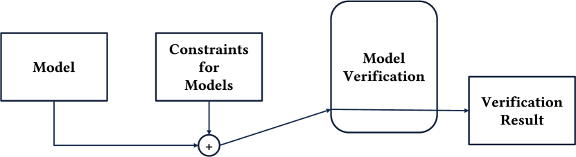
(a) Approach for verifying a single model against a set of correctness constraints.

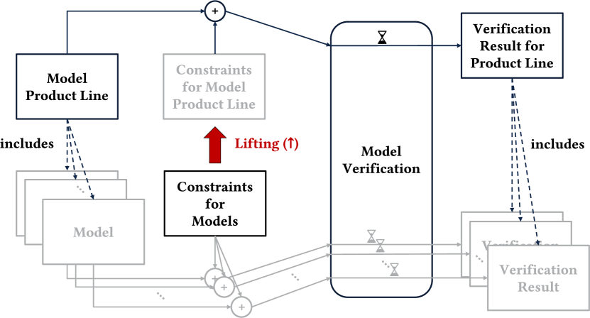
(b) Our approach for model product-lines is to automatically lift constraints, such that they apply for the model product-line. With this we can verify the product-line by using the same verification without having to verify the single model variants.

Figure 1. Motivation and concept for our lifting approach.

Many of today’s products are produced as multiple different product variants. Some reasons for this variability in products arise from customers’ demands, others from different regional situations within a global market. Also a company’s individual portfolio management strategy is reflected, here. To address this situation, (software) product-line engineering provides a methodology to develop multiple variants simultaneously, such that the same development artifacts can be reused among as many variants as required.

To do so, one classically develops a collection of reusable artifacts from which individual product variants can be generated as comfortably as possible – ideally automatized. The development of such common artifacts (domain artifacts) - the so-called domain engineering - is for example explained by Pohl et al. (Pohl et al., 2005).

The number of different variants that can be generated this way often gets very large, as it grows exponentially with the number of optional product features. Already 33 independent optional features allow $2^{33}$ (more than 8.5 billion) configurations – an individual variant for every human being on Earth. Though this demonstrates the potential power of this approach, it also causes problems, especially for verification. Classical testing of such a product-line requires to check a variant once it is generated.

For many application domains however, one cannot afford to wait until a variant is generated to discover errors. An example is a car for which the manufacturer only realizes during production that certain combinations of configuration options are incompatible. Furthermore, for the usually high number of variants, checking each and everyone individually would not even be possible. The prominent example of the Linux Kernel comprises more than 10.000 features (Lotufo et al., 2010) – compiling and testing every combination individually is impossible, here. Also the study (Rhein et al., 2018) by Rhein et al. illustrates this scalability issue with five real software product-lines. It demonstrates the ineffectiveness of such checks variant by variant, even for low numbers of variants.

Due to these problems of early verification and scalability, one would ideally like to check the domain artifacts of a product-line for correctness before even generating variants. This approach is called product-line analysis – a technique and methodology that was mainly developed for software or software-intensive products. This is why there are several analysis techniques that deal with the verification of specific software related issues – type checking as by Kastner et al. (Kästner et al., 2012) is a prominent example, here.

For model-based engineering however, developing such specific analysis algorithms is less efficient, since different modeling languages might differ strongly from each other – both in syntax and semantics. While this makes it especially hard to transfer product-line analysis methods from one modeling language to another, the development of dedicated analysis algorithms for each modeling language is neither trivial nor efficient.

To overcome this problem with reusing specific analysis mechanisms, there are generic solutions in model-based engineering. The usual solution hereby is the usage of generic constraint checkers to verify correctness constraints on a model, as illustrated in Figure 1(a). An example for such a constraint in systems engineering could be “All incoming signals of all subsystems need to be provided values which match the type which is defined in the subsystems interfaces.”

If there however is variability in models, we deal with model product-lines and several model variants. As indicated in Figure 1(b), the usage of generic constraint checkers for individual model variants becomes less efficient. Here, every model variant will require time and effort to be verified individually and the same scalability and early verification issues arise, that are described above.

In this work, we present a way to use generic verification mechanisms to implement a reusable product-line analysis for arbitrary modeling languages. With our approach, it becomes sufficient to just specify correctness constraints for individual (i.e. non-variable) model variants. The corresponding product-line analysis can then be obtained “for free”. This can especially be helpful for the development of (new) domain specific modeling languages.

Figure 1(b) gives an overview about our approach. The key idea is to automatically adapt (“lift”) constrains that are supposed to be correct for the individual model variants, such that they apply to the model product-line. We do this constraint lifting in such a way that a lifted constraint holds for a model product-line iff the original constraint will hold for all variants. With this, a lifted constraint can be checked on the model product-line – just as it would have been done for individual models. Hereby classical generic verification mechanisms can be modularly utilized. Prominent possibilities are SMT solving or even theorem proving, if the base theories used the constraint language are not decidable. In case of SMT solvers, the verification result can be a counterexample in form of a variant that violates a constraint.

In a case study we apply our approach to a modeling language for production planning by lifting its constraints. We present a generic product-line analysis by means of an automated translation of model product-lines from the Eclipse Modeling Framework (EMF) to SMT. This analysis is used to translate two industrial model product-lines for the SMT solver Z3 to verify the lifted constraints. With this, the case study not only illustrates our approach, but also demonstrates the scalability with a runtime analysis.

The rest of the paper is organized as follows: A notion of modeling and constraint languages with a corresponding formalization (formalism is required for the lifting and the translation to the verification mechanism) is introduced in Section 3. Section 4 extends these notions by introducing variability in models and presents the lifting function for constraints. The SMT translation, the industrial case study and the runtime analysis are presented in Section 5. The paper concludes with the Sections 6 on related work and  7 on conclusion and future work.

2. Running Example

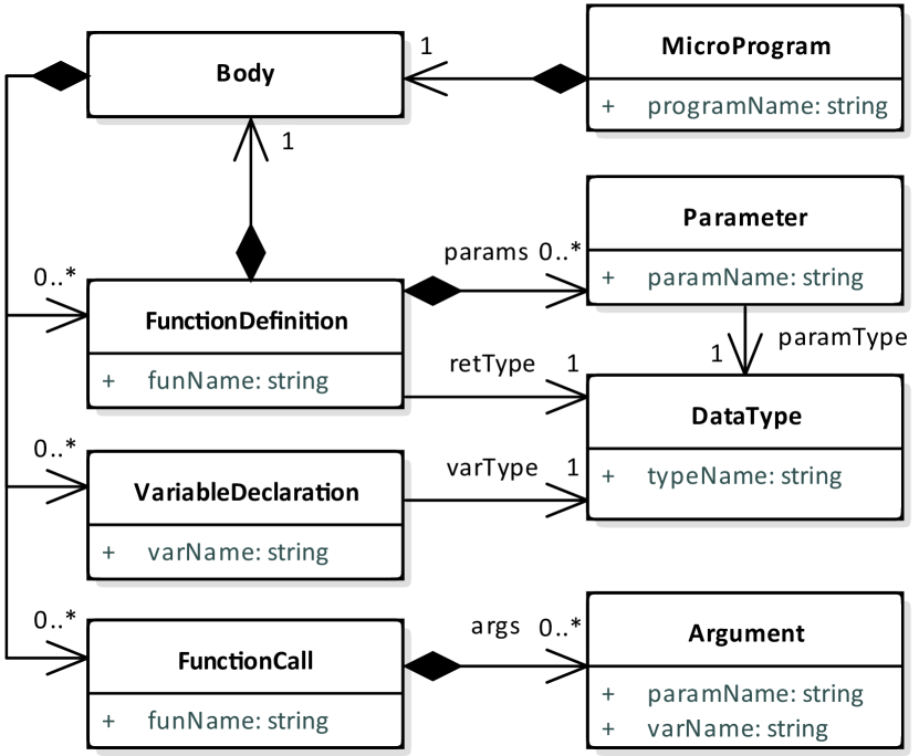
Figure 2. Metamodel for our running example: the modeling language $\mu L$.

The approach for analyzing model product-lines in this paper is independent of a concrete modeling language. As a running example for the notions throughout the paper, we now introduce one modeling language for illustrating purposes.

It is simple language, that models function declarations, function calls and variables - we call this language Micro Language ($\mu L$). The metamodel of $\mu L$ is given in Figure 2.

For a convenient presentation, we chose a textual syntax that is similar to C or Java. A small $\mu L$ program is given in Figure 3 (textual) and 4 (object diagram).

In this language, a correctness constraint could be type correctness. This means, that the Arguments of all FunctionCalls need to have the same DataType, as the corresponding Parameter. $myProgram1$ of Figure 3 is correct with respect to this constraint. A counterexample is given in Figure 5. Here, the FunctionCall will invoke an integer function with a float parameter in line 7.

Section 3.3 will formally define such constraints for this example and Section 4.1 will enhance the example with variability. Actually, there will also be Figure 7 that shows a product-line, which contains the presented example models of Figures 3 and 5 as variants.

⬇

1Program myProgram1 // program

2{ // body

3 Var integer myVar; // var

4

5 myFun( // callMyFun

6 p1=myVar); // arg

7

8 Fun integer myFun( // fun

9 integer p1) // p1

10 { [...] }}

Figure 3: A simple example model in textual syntax. The corresponding object diagram can be found in Figure 4. Some object names are annotated here in comments.

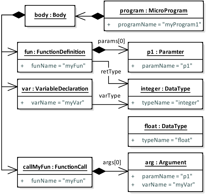
Figure 4. The example model “myProgram1” as an object diagram. The textual representation is given in Figure 3.

⬇

1Program myProgram2

2{

3 Var float myVar;

4

5 // Here a float variable is passed to an integer

6 // parameter. A violation of the type constraint

7 myFun(p1=myVar);

8

9 Fun integer myFun(integer p1) {

10 [...] }}

Figure 5: A $\mu L$ program, that violates the type correctness constraint for function calls.

3. Metamodels, Models and Constraints

In this section, we introduce the necessary formal basis for the rest of the paper: metamodel, model, constraint language. These are the basic notions to deal with, when specifying a modeling language: constraints will be specified on the level of metamodels and are checked on models to verify their correctness.

This chapter does not deal with variability: here we first introduce the non-variable case as a baseline and later focus on variability and product-lines in a dedicated Section 4.

3.1. Metamodel

We now formalize various necessary notions of metamodeling in an usual way. Let $\mathbb{I}$ be a set of identifiers (typically a set of strings in our examples). Let $\mathbb{T}\subseteq\mathbb{I}$ be a set of type identifiers such that $int,bool,string\in\mathbb{T}$. We call $int,bool,string$ the basic types of $\mathbb{T}$ (we omit other potential basic types like floats for the sake of simplicity). The domain for these basic types is $\mathbb{B}$ for $bool$, $\mathbb{Z}$ for $int$ and the set of all strings $\mathbb{S}$ for $string$. A multiplicity is an element of $\mathbb{M}\stackrel{{\scriptstyle\text{def}}}{{=}}\{1,*\}$ (we omit other potential multiplicities for the sake of simplicity). The set of attributes $\mathbb{A}$ is defined as the set of tuples of $\mathbb{T}\times\mathbb{M}$. The set $\mathbb{C}$ of class bodies is defined as the set of finite functions of $\mathbb{I}\to\mathbb{A}$. The set $\mathbb{M}_{meta}$ of metamodels is defined as the set of finite functions of $\mathbb{T}\to\mathbb{C}$. A metamodel $M\in\mathbb{M}_{meta}$ is well-defined iff every type referred in $M$ is also a type defined in $M$. We will only consider well-defined metamodels in the following. Note that we formalize associations slightly different than often done, by formalizing them simply like the attributes above, which can have a non-basic type. This makes the formalization simpler and does not entail any loss of generality.

Example. For the metamodel of Figure 2 this means: $\displaystyle int,string,Body,FunctionDefinition,funName$ $\displaystyle\in\mathbb{I}$ $\displaystyle int,string,Body,FunctionDefinition$ $\displaystyle\in\mathbb{T}$ $\displaystyle(string,1),(Body,1),(FunctionDefinition,*)$ $\displaystyle\in\mathbb{A}$ $\displaystyle FunctionDefinition_{cb},MicroProgram_{cb}$ $\displaystyle\in\mathbb{C}$ $\displaystyle FunctionDefinition_{cb}=\langle funName\mapsto(string,1),$ $\displaystyle\hskip 19.91684ptparams\mapsto(Parameter,*),retType\mapsto(DataType,1)\rangle$ $\displaystyle FunctionDefinition_{cb}(params)=(Parameter,*)$ $\displaystyle MicroProgram_{cb}=\langle programName\mapsto(String,1),\ldots\rangle$ $\displaystyle\mu L\in\mathbb{M}_{meta}$ $\displaystyle\mu L=\langle FunctionDefinition\mapsto FunctionDefinition_{cb},$ $\displaystyle\hskip 28.45274ptMicroProgram\mapsto MicroProgram_{cb},\ldots\rangle$ $\displaystyle\mu L(FunctionDefinition)=FunctionDefinition_{cb}$

3.2. Core Model

We now define instances of a metamodel as well as the corresponding notions. In order to distinguish between non-variable models and the model product-lines of Section 4, we denote models without variability as core models.

Definition 3.1 (Instances).

Let $M\in\mathbb{M}_{meta}$ be a metamodel and $t\in\mathbb{T}$ be a type defined in $M$. The set $Inst_{M}(t)$ of the instances of $t$ in $M$ is inductively defined as follows:

$$Inst_{M}(t)\stackrel{{\scriptstyle\text{def}}}{{=}}\begin{cases}\mathbb{B}&\text{if }t=bool\\ \mathbb{Z}&\text{if }t=int\\ \mathbb{S}&\text{if }t=string\\ \mathbb{O}_{M}(t)&\text{else}\\ \end{cases}$$

where the set $\mathbb{O}_{M}(t)$ of objects for a type $t$ in metamodel $M$ is defined as:

$$\mathbb{O}_{M}(t)\stackrel{{\scriptstyle\text{def}}}{{=}}\{f|f(id)\in Inst^{\mathbb{A}}_{M}(a)\text{ s.t. }$$

$$\hskip 11.38109pt\exists id\in\mathbb{I},a\in\mathbb{A},c\in\mathbb{C}.$$

$$\hskip 11.38109ptM(t)=c\wedge c(id)=a\}$$

with $Inst^{\mathbb{A}}_{M}(a)$ for an attribute $a=(t,m)$ defined as:

$$Inst^{\mathbb{A}}_{M}((t,m)) \stackrel{{\scriptstyle\text{def}}}{{=}}\begin{cases}Inst_{M}(t)&\text{if }m=1\\ \mathbb{L}(Inst_{M}(t))&\text{if }m=*\\ \end{cases}$$

where $\mathbb{L}(S)$ denotes the set of lists of elements of a set.

We write $Inst_{M}$ for the set of all models of a metamodel $M$, i.e. $Inst_{M}\stackrel{{\scriptstyle\text{def}}}{{=}}\{m|\exists t\in\mathbb{T}.m\in Inst_{M}(t)\}$.

Example for Definition 3.1. The $\mu L$ model of Figure 4 would be: $\displaystyle Inst_{\mu L}(bool)=\{true,\ false\}$ $\displaystyle\langle typeName\mapsto\text{``float''}\rangle\in Inst_{\mu L}(DataType)$ $\displaystyle\langle typeName\mapsto\text{``integer''}\rangle\in Inst_{\mu L}(DataType)$ $\displaystyle\langle typeName\mapsto\text{``integer''}\rangle\in Inst_{\mu L}$ $\displaystyle\langle funName\mapsto\text{``myFun''},$ $\displaystyle\ \ \ retType\mapsto\langle typeName\mapsto\text{``integer''}\rangle,$ $\displaystyle\ \ \ params\mapsto[\langle paramName\mapsto\text{``i1''},$ $\displaystyle\hskip 54.06006ptparamType\mapsto\langle typeName\mapsto\text{``integer''}\rangle\rangle]$ $\displaystyle\ \rangle\in Inst_{\mu L}(FunctionDefinition)$

3.3. Constraint Language

After we have introduced metamodels and their models, we continue to the constraint language. A constraint language allows to restrict the set of instances of a metamodel which are considered valid. For example, think back to the $\mu L$ program $myProgram2$ of Figure 5 with the incorrectly typed function call: even though it is an instance of the $\mu L$ metamodel, it is invalid due to the type error.

In metamodeling, constraints are classically expressed by OCL invariants. In our case - to simplify the algorithms - we define our own constraint language based on first order (predicate) logic. This is not a limitation, since OCL invariants can be translated to first-order logic, as for example presented by Beckert et al. (Beckert et al., 2002).

An essential aspect is that we parameterize our language with a base (first-order) theory defining the atoms of the language. For instance, one can consider atoms that allow list expressions like $arguments.size=parameters.size$, or arithmetic expressions, etc.. We will also see these two theories in the SMT implementation of therefore left undefined for our constraint language, which focuses only on composing such atoms into complex constraints.

Definition 3.2 (Constraint Language $\mathcal{L}$).

Let $B_{1},\ldots,B_{k}$ be a set of base theories. The constraint language $\mathcal{L}(B_{1},\ldots,B_{k})$ (or simply $\mathcal{L}$ when $B_{1},\ldots,B_{k}$ are clear from the context) is defined by the following grammar:

$$\mathcal{L} \stackrel{{\scriptstyle\text{def}}}{{=}} < >$$ QEXPR

$$< > \stackrel{{\scriptstyle\text{def}}}{{=}} \forall\text{{$<$}VAR$>$}\in\text{{$<$}SET$>$}:\text{{$<$}EXPR$>$}$$QEXPR

$$< > \stackrel{{\scriptstyle\text{def}}}{{=}} [a-zA-Z]^{+}$$VAR

$$< > \stackrel{{\scriptstyle\text{def}}}{{=}} \mathbb{T}\ |\ \text{{$<$}NAV$>$}$$SET

$$< > \stackrel{{\scriptstyle\text{def}}}{{=}} \text{{$<$}VAR$>$}\ |\ \text{{$<$}NAV$>$}.\mathbb{I}$$NAV

$$< > \stackrel{{\scriptstyle\text{def}}}{{=}} \text{{$<$}ATOM$>$}\ |\ \text{{$<$}QEXPR$>$}\ |\ \neg\ \text{{$<$}EXPR$>$}\ |$$EXPR

$$\ \text{{$<$}EXPR$>$}\vee\text{{$<$}EXPR$>$}$$

$$< > \stackrel{{\scriptstyle\text{def}}}{{=}} A_{1}\ |\ ...\ |\ A_{j}$$ATOM

where $A_{1},...,A_{j}$ are arbitraty atoms of the base theories $B_{1},\ldots,B_{k}$. An example for such an atom, would again be the afore mentioned term $arguments.size=parameters.size$.

For brevity we only defined the $\forall$ quantifier and the Boolean operators $\vee$ and $\neg$ – of course this is not a limitation and in the following, we also use $\exists,\ \wedge$ and $\implies$ as “syntactic sugar”.

Example for Definition 3.2. $\mathcal{L}$ constraints for $\mu L$ could be:
“All function names are unique”: $\displaystyle\forall$ $\displaystyle f_{1}\in FunctionDefinition:$ $\displaystyle\neg\exists f_{2}\in FunctionDefinition:$ $\displaystyle\ f_{1}\neq f_{2}\ \wedge\ f_{1}.funName=f_{2}.funName$ All arguments use only variables, which are defined: $\displaystyle\forall$ $\displaystyle a\in Argument:\exists v\in VariableDeclaration:$ $\displaystyle a.varName=v.varName$ “All types of all variables used in all arguments of all calls, match with the type of the respective parameters”: $\displaystyle\forall$ $\displaystyle F_{call}\in FunctionCall:\forall a\in F_{call}.args:$ $\displaystyle\exists$ $\displaystyle F_{def}\in FunctionDefinition:\forall p\in F_{def}.params:$ $\displaystyle\exists$ $\displaystyle v\in VariableDeclaration:$ $\displaystyle a.paramName=p.paramName\ \wedge$ $\displaystyle a.varName=v.varName\implies$ $\displaystyle v.varType=p.paramType$

4. Model Product-Lines and Constraint Lifting

In the previous section, we described modeling languages with metamodels and constraints. Hereby (core) models are the instances of metamodels that shall fulfill all specified constraints.

Whenever there is a need for several variants of a model, one usually does not want to maintain several copies of it, individually. Instead, one can systematically capture the respective variability within the model, such that the variants can be automatically generated, whenever needed. With such variability in a model, we speak of a model product-line.

This section will first extend the notion of core models to model product-lines. After that, it will present our approach of how constraints can simultaneously be checked for all variants of such a model product-line.

4.1. Variability in Models

To formalize variability, we utilize the usual feature model notion as introduced by Kang et al. (Kang et al., 1990). Let $F$ be the set of all features, then $\Phi_{F}$ a feature model over $F$. As there is plenty of work on how to formalize feature models, we do not further go into details and consider $\Phi_{F}$ as being a propositional logic formula that encodes which feature configurations are allowed. For more details on how to formalize $\Phi_{F}$ itself and on how to translate feature models to propositional logic formulas, see e.g. Batory et al. (Batory, 2005). Section 5 will also show an example for such a formula.

Figure 6. A feature model for the product-line of $\mu L$ programs in Figure 7.

Example. An example for a feature model is given in Figure 6. The product-line here offers different variants of a $\mu L$ program. Here, the program’s variants differ, depending on whether the executing hardware platform comprises a floating point unit (feature FPU) or not. Furthermore, for every variant, one needs to select an optimization (feature SoftwareOptimization). One of the optimization alternatives focuses on runtime efficiency (feature Runtime), the other optimization on precision (feature Precision). However, to make the high precision possible, the feature FPU needs to be selected, too (constraint requires). For this feature model the set of features is: $\displaystyle F$ $\displaystyle=$ $\displaystyle\{SoftwareOptimization,ControllerFeatures,Precision,$ $\displaystyle\ Runtime,FPU\}$

The features of the feature model shall now be used to track variability in a model product-line. A usual approach here, is to annotate model elements with so called presence conditions - i.e. terms that specify to which features or feature combinations an annotated element belongs.

The set $\mathbb{P}_{F}$ of presence conditions over a set of features $F$ is defined as the set of propositional logic formulas whose atomic propositions are elements of $F$.

Definition 4.1 (Presence Condition Function).

A presence condition function $\lambda:Inst_{M}\to\mathbb{P}_{F}$ assigns presence conditions to model elements $m\in Inst_{M}$.

⬇

1Program myProgramProductLine {

2 Var float myVar; [FPU]

3 Var integer myVar; [!FPU]

4

5 myFun(p1=myVar);

6

7 Fun integer myFun(integer p1) [!FPU | Runtime]

8 { [...] }

9 Fun float myFun(float p1) [FPU & Precision]

10 { [...] }}

Figure 7: A $\mu L$ product-line, annotated with the features from Figure 6. Selecting the features FPU and Runtime at the same time will result in the incorrect variant of Figure 5.

Example for Definition 4.1. We now informally extend the example modeling language $\mu L$ with variability. In the textual representation, features can be added to language constructs by adding a subsequent term of the syntax [$<$presence condition$>$]. In Figure 7 there is a $\mu L$ program, for which there shall be different variants according to the feature model of Figure 6. Depending on whether the executing hardware comprises a floating point unit (feature FPU), the program uses the datatype float - otherwise only integer. For runtime optimized execution (feature Runtime) the function myFun is declared using integer - otherwise float is used, in cases in which the feature FPU is available. For the $\mu L$ program of Figure 7, some examples for $\lambda$ are: $\displaystyle\lambda(\text{{\color[rgb]{0.7265625,0,0.33203125}Var float} myVar;})$ $\displaystyle=FPU$ $\displaystyle\lambda(\text{{\color[rgb]{0.7265625,0,0.33203125}Var integer} myVar;})$ $\displaystyle=\neg FPU$ $\displaystyle\lambda(\text{{\color[rgb]{0.7265625,0,0.33203125}Fun integer} myFun({\color[rgb]{0.7265625,0,0.33203125}integer} p1)})$ $\displaystyle=\neg FPU\ \vee\ \text{Runtime}$ $\displaystyle\lambda(\text{myFun(p1=myVar);})$ $\displaystyle=true$

Definition 4.2 (Model Product-Line).

A model product-line is a triple $(m,\Phi_{F},\lambda)$, where $m$ is a model, $\Phi_{F}$ is a feature model with a set of features $F\subseteq F$ and $\lambda$ is a presence condition function for $m$.

Definition 4.3 (Configuration).

A configuration is as a function $k_{\Phi_{F}}:F\to\mathbb{B}$ such that $k_{\Phi_{F}}\models\Phi_{F}$.

This means that a configuration selects features by assigning Boolean values to each of them. According to this definition, $k_{\Phi_{F}}$ is always a valid configuration, i.e., satisfying all constraints of the feature model.

Example for Definition 4.3. One possible configuration for $\Phi_{F}$ could be: $\displaystyle k_{\Phi_{F}}(f)$ $\displaystyle=\begin{cases}\text{true}&\text{if }f\in\parbox[t]{216.81pt}{\{SoftwareOptimization, ControllerFeatures, Runtime, FPU\}}\\ \text{false}&\text{else}\\ \end{cases}$

4.2. Symbolic Binding of Product-line Variability

The introduced notions describe how to specify a model product-line by means of a core model and a presence condition function. The objective of this paper is to simultaneously check constraints for all variants of such a model product-line – i.e. product-line analysis. To accomplish this, it is important to understand the effect of the presence conditions for the core model.

In this section, we will describe and formalize this effect in what we denote as symbolic binding. This formalism is necessary as an auxiliary technique or preprocessing step that will be part of the lifting-based product-line analysis in this paper. The idea behind symbolic binding, is to encode all variability that a presence condition function $\lambda$ might specify for a core model $m$, immediately into one symbolic representation $m\downarrow$ of all possible variants. Figure 8 illustrates this refined overview of our concept, including all of these notions.

Definition 4.4 (Binding Function $\downarrow$).

Given a model product-line $(m,\Phi_{F},\lambda)$ the symbolic binding function $\downarrow_{k}$ maps the model $m$ to a model $m\downarrow_{k}$ for arbitrary configurations $k$ s.t. $k\vDash\Phi_{F}$ as follows:

$$m\downarrow_{k}\stackrel{{\scriptstyle\text{def}}}{{=}}\begin{cases}m&\text{if }m\in\mathbb{B}\cup\mathbb{Z}\cup\mathbb{S}\\ \begin{cases}m\downarrow_{\mathbb{O}k}&\text{if }k\vDash\lambda(m)\\ \bot&\text{else}\\ \end{cases}&\text{if }m\in\mathbb{O}_{M}\end{cases}$$

where $m\downarrow_{\mathbb{O}k}$ is the binding function for objects $m\in\mathbb{O}_{M}$ with $m=\{f_{1},\ldots,f_{n}\}$ that is defined as:

$$m\downarrow_{\mathbb{O}k}\stackrel{{\scriptstyle\text{def}}}{{=}}\{f_{1}\downarrow\ldots f_{n}\downarrow\}$$

where

$$f\downarrow(id)\stackrel{{\scriptstyle\text{def}}}{{=}}\begin{cases}\begin{cases}f(id)&\text{if }k\vDash\lambda(f(id))\\ \bot&\text{else}\\ \end{cases}&\text{if }f(id)\in Inst_{M}\\ l\in\mathbb{L}(Inst_{M})\text{, where }\forall e\in l.&\\ \hskip 11.38109pte\in f(id)\wedge k\vDash\lambda(e)&\text{if }f(id)\in\mathbb{L}(Inst_{M})\end{cases}$$

Intuitively speaking, this binding inserts if-then-else constructs as a distinction of cases for the existence of referred objects. An association to an optional object will refer to this object only if its presence condition is true - and to $\bot$, else. Analogously for list associations: an object will be in a variants list iff the objects presence condition evaluates to true.

Note that throughout this definition, the configuration $k$ remains a free parameter. This is why we denote these functions as symbolic binding functions. They could be used to actually generate a variant by instantiating $k$ with a concrete configuration. In the context of this work, the intention is to let a solver reason over all configurations (Section 5.1 will show an exemplary SMT translation).

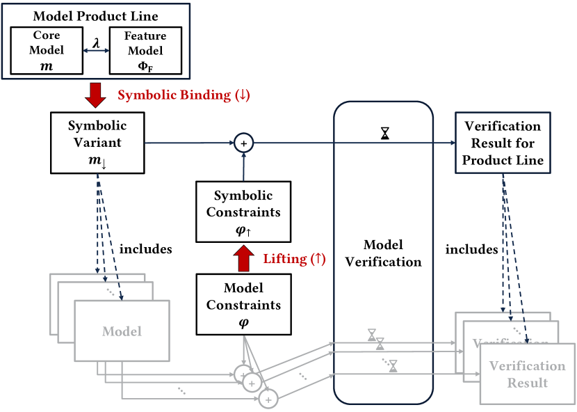
Figure 8. Refined approach for verifying a model product-line by symbolic binding.

4.3. Lifting Constraints to Symbolic Variant Level

The introduction of variability into a model entails that the resulting model product-line contains model elements for several variants at the same time. Since the constraints for the modeling language however specify correctness for individual models, they usually do not apply for model product-lines anymore.

Our solution to re-enable constraint verification on model product-lines is the constraint lifting. It automatically performs an extension to the constraints by means of the lifting function $\uparrow$:

Definition 4.5 (Lifting Function $\uparrow$).

Let $(m,\Phi_{F},\lambda)$ be a model product-line, the lifting function $.\uparrow:\mathcal{L}\to\mathcal{L}$ is inductively defined:

$$(\forall v\in set:expr)\uparrow \stackrel{{\scriptstyle\text{def}}}{{=}}\begin{cases}\forall v\in set:\lambda(v)\implies expr\uparrow&\text{if }set\in\mathbb{T}\\ \forall v\in set:expr\uparrow&\text{else}\\ \end{cases}$$

$$(expr_{1}\vee expr_{2})\uparrow \stackrel{{\scriptstyle\text{def}}}{{=}}expr_{1}\uparrow\ \vee\ expr_{2}\uparrow$$

$$(\neg expr)\uparrow \stackrel{{\scriptstyle\text{def}}}{{=}}\neg(expr\uparrow)$$

$$nav\uparrow \stackrel{{\scriptstyle\text{def}}}{{=}}nav$$

The result of $\phi\uparrow$ is again a constraint.

The intuition behind this is that a constraint only needs to hold for combinations of model elements that are selected at the same time. Hence, the key is the first rule: An expression that specifies an invariant for certain model elements only needs to hold for those model elements whose presence condition evaluates to true.

For syntactic sugar, one can rewrite these rules, of course. For example, the rule for the $\exists$ quantor follows immediately from the $\forall$ and $\neg$ lifting rules.

Example for Definition 4.5. When lifting the constraints of the example from Definition 3.2, $\uparrow$ results in (changes highlighted): “All function names are unique”: $\displaystyle(\forall$ $\displaystyle f_{1}\in FunctionDefinition:$ $\displaystyle\neg$ $\displaystyle\exists f_{2}\in FunctionDefinition:$ $\displaystyle f_{1}\neq f_{2}\ \wedge\ f_{1}.funName=f_{2}.funName)\uparrow$ $\displaystyle=\forall$ $\displaystyle f_{1}\in FunctionDefinition:$ $\displaystyle\text{{\color[rgb]{0,0,0}\text@underline{$\lambda_{(}f_{1})\implies$}}}\neg\exists f_{2}\in FunctionDefinition:$ $\displaystyle\text{{\color[rgb]{0,0,0}\text@underline{$\lambda(f_{2})\ \wedge$}}}\ f_{1}\neq f_{2}\ \wedge\ f_{1}.funName=f_{2}.funName$ “All given arguments are defined”: $\displaystyle(\forall$ $\displaystyle a\in Argument:\exists v\in VariableDeclaration:$ $\displaystyle a.varName=v.varName)\uparrow$ $\displaystyle=\forall$ $\displaystyle a\in Argument:\text{{\color[rgb]{0,0,0}\text@underline{$\lambda(a)\implies$}}}\exists v\in VariableDeclaration:$ $\displaystyle\text{{\color[rgb]{0,0,0}\text@underline{$\lambda(v)\ \wedge$}}}\ a.varName=v.varName$ “All types of all variables used in all arguments of all calls, match with the type of the respective parameters”: $\displaystyle(\forall$ $\displaystyle F_{call}\in FunctionCall:\forall a\in F_{call}.args:$ $\displaystyle\exists$ $\displaystyle F_{def}\in FunctionDefinition:\forall p\in F_{def}.params:$ $\displaystyle\exists$ $\displaystyle v\in VariableDeclaration:$ $\displaystyle a.paramName=p.paramName\ \wedge$ $\displaystyle a.varName=v.varName\implies$ $\displaystyle v.varType=p.paramType)\uparrow$ $\displaystyle=\forall$ $\displaystyle F_{call}\in FunctionCall:\text{{\color[rgb]{0,0,0}\text@underline{$\lambda(F_{call})\implies$}}}\forall a\in F_{call}.args:$ $\displaystyle\exists$ $\displaystyle F_{def}\in FunctionDefinition:\text{{\color[rgb]{0,0,0}\text@underline{$\lambda(F_{def})\ \wedge$}}}\ \forall p\in F_{def}.params:$ $\displaystyle\exists$ $\displaystyle v\in VariableDeclaration:$ $\displaystyle\text{{\color[rgb]{0,0,0}\text@underline{$\lambda(v)\ \wedge$}}}\ (a.paramName=p.paramName\ \wedge$ $\displaystyle a.varName=v.varName\implies$ $\displaystyle v.varType=p.paramType)$

Note that in Definition 4.5 e.g. the last rule “$nav\uparrow\stackrel{{\scriptstyle\text{def}}}{{=}}nav$” for navigation expressions can only be that simple, since these constraints are applied on models by means of the symbolic binding. This means loosely speaking that navigation expressions can only reach model elements that are present, since the binding already made references and attributes symbolically dependent from their presence condition. This also applies to the second case of the quantifier rule, where $set$ is not a type, but some navigation expression.

5. Case Study: A DSML for Manufacturing Planning

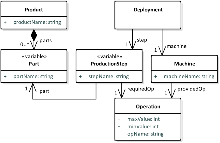
Figure 9. Simplified metamodel of the SFIT language.

In the previous sections, we introduced the lifting approach and applied it to the $\mu L$ language, as a running example. In this case study, we apply it to the SFIT modeling language for production planning, that we introduced in (Bayha et al., 2016). We not only present the language and the result of lifting their constraints, but also show how we use SMT solving for product-line analysis in Section 5.1. Finally, Section 5.2 gives a runtime analysis for SFIT model product-lines in order to evaluate the scalability of our approach.

The motivation for the SFIT modeling language comes from the production planning departments of two industry partners. Both companies want to check whether their factories are capable of producing all variants of their products. To this end, the SFIT language models all aspects, that are relevant for answering this producablity question. These modelled aspects are the product to be manufactured, as well as the corresponding production process and the available assembly lines. Since the products as well as the production processes are variable, these SFIT models are model product-lines that can be analyzed using our approach.

For the presentation of the metamodel and constraints in this paper, we use a simplified version of the metamodel that can be seen in Figure 9. The complete modeling language is larger and defined by a metamodel of about 40 classes. But already the simplified version here is representative, as it contains the essence of how we modeled the major use case of our industry partners.

In this simplified metamodel, the product is represented by the classes Product and Part. The production process is modeled by the ProductionStep class and the assembly lines components correspond to the Machine class. Both – ProductionSteps and Machines – have an association to an Operation class that is required in the ProductionStep and provided by the Machine. Finally, a Deployment class describes the mapping of ProductionSteps to Machines.

For the case study we only allow variability for the classes Part and ProductStep (indicated by the stereotype ¡¡variable¿¿). We do this distinction here only for readability of the code fragments. Besides this, such limitations are out of the scope of this paper, however they also do not conflict with our approach.

Some correctness constraints to ensure producability are:

Constraint 1: “All ProductionSteps are deployed to a Machine”:

$$\forall s\in ProductionStep:$$

$$\exists d\in Deployment:d.step=s$$

Constraint 2: “For all Parts of all Products, there is a ProductionStep that assembles the Part”:

$$\forall prod\in Product:\forall part\in prod.parts:$$

$$\exists step\in ProductionStep:$$

$$\hskip 7.11317ptstep.assembledPart=part$$

Constraint 3: “All ProductionSteps are deployed to a Machine, that can fulfill the ProductionSteps required Operation”:

$$\forall d \in Deployment:$$

$$d.step.requiredOp.name=$$

$$d.machine.providedOp.name$$

$$\wedge( d.step.requiredOp.maxValue\geq$$

$$d.machine.providedOp.minValue$$

$$\vee d.step.requiredOp.minValue\leq$$

$$d.machine.providedOp.maxValue)$$

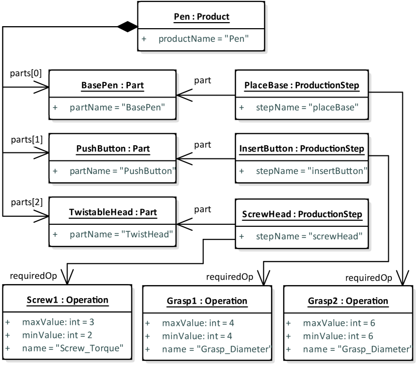
(a) The product and the corresponding production process.

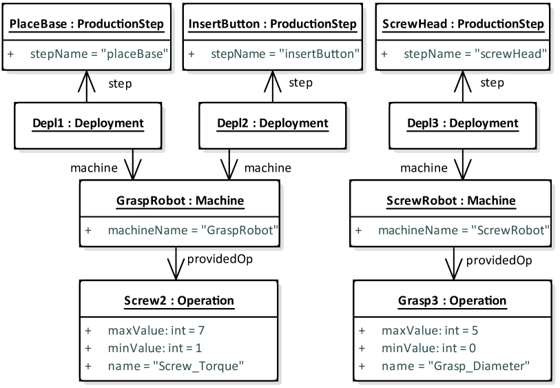
(b) A mapping of the above production process to Machines.

Figure 10. A simple SFIT model for manufacturing pens.

5.1. Product-line Analysis using SMT Solving

After introducing the modeling language for the case study, we now show how we implemented our approach using the SMT solver Z3 (De Moura and Bjørner, 2008). Hereby, model product-lines and constraints are automatically translated to SMT to be analyzed. This translation itself is independent of SFIT and translates arbitrary models of the Eclipse Modeling Framework (EMF) to SMT using the Z3 Java API.

We use an illustrative SFIT model product-line that captures how a product-line of pens is manufactured. It can be seen in Figure 10(a) and 10(b). This model comprises parts and production steps for two variants of pens - one variant with a push button as opening mechanism; one variant with a twist mechanism. A feature model that captures this variability can be seen in the following SMT translation of a formula $\Phi_{F}$ of Section 4.1 in SMT-LIBv2 syntax (Cok et al., 2011):

⬇

1(declare-const PenFeatures bool)

2(declare-const OpenMechanism bool)

3(declare-const TwistToOpen bool)

4(declare-const PushToOpen bool)

5

6(assert (=> OpenMechanism PenFeatures))

7(assert (=> OpenMechanism (or PushToOpen TwistToOpen)))

8(assert (=> PushToOpen OpenMechanism))

9(assert (=> TwistToOpen OpenMechanism))

10(assert (=> TwistToOpen (not PushToOpen)))

11(assert (=> PushToOpen (not TwistToOpen)))

12(assert (=> PenFeatures OpenMechanism))

13(assert (= PenFeatures true))

As one can see, Features are translated as uninterpreted bool constants. The feature tree structure and the requires relation are expressed by the implications in lines 6 to 13.

Classes and objects are naturally translated as datatypes and datatype entities. Also the presence condition function $\lambda$ can be translated straight forward, as can be seen in the function selected_part for Part objects here:

⬇

1(declare-datatypes ()(

2 (Part BasePen PushButton TwistableHead NONE_Part)))

3

4(declare-fun selected_part (Part) Bool)

5(assert (= (selected_part BasePen) true))

6(assert (= (selected_part PushButton) PushToOpen))

7(assert (= (selected_part TwistableHead) TwistToOpen))

Note, that for the datatype Part, there also is an element NONE_Part. This corresponds to the usual notion of $\bot$ respectively null

Associations are formalized as functions in Section 3. They are also translated like this in SMT. The following SMT code results for the associations step and machine of class Deployment:

⬇

1(declare-fun Deployment_step (Deployment) ProductionStep)

2(declare-fun Deployment_machine (Deployment) Machine)

3

4(assert (= (Deployment_step Depl1)

5 (ite (selected_step PlaceBase) PlaceBase NONE_Step)))

6(assert (= (Deployment_machine Depl1) GraspRobot))

7(assert (= (Deployment_step Depl2)

8 (ite (selected_step InsertButton) InsertButton NONE_Step)))

9(assert (= (Deployment_machine Deplt2) GraspRobot))

10(assert (= (Deployment_step Depl3)

11 (ite (selected_step ScrewHead) ScrewHead NONE_Step)))

12(assert (= (Deployment_machine Depl3) ScrewRobot))

Here, one can also see the symbolic binding of variability using the SMT construct ite (“if-then-else”) - just as in Definition 4.4.

Symbolic binding is also relevant for list associations. In SMT, we use sequences and concatenation to form symbolic lists – depending on the selection function, list members are translated either as one-element-sequences or empty sequences. With this, the list association parts between the classes Product and Part results in:

⬇

1(declare-fun Prod_parts (Product) (Seq Part))

2

3(assert (= (Prod_parts Pen) (seq.++

4 (ite (selected_part BasePen)

5 (seq.unit BasePen)

6 (as seq.empty (Seq Part)))

7 (ite (selected_part PushButton)

8 (seq.unit PushButton)

9 (as seq.empty (Seq Part)))

10 (ite (selected_part TwistableHead)

11 (seq.unit TwistableHead)

12 (as seq.empty (Seq Part))))))

Correctness constraints are already expressed in first order logic. We only need to negate them in order to let the SMT solver try to find one variant among all possible feature configurations that violates the constraint. Without this negation, the solver would search for one feature configuration that fulfills all constraints instead of checking all variants for one violation. The constraint “All ProductionSteps are deployed to a Machine” is lifted and translated:

⬇

1(exists ((s ProductionStep))

2 (and

3 (selected_step s)

4 (forall ((d Deployment)) (not(= (Deployment_step d) s)))))

The constraint “For all Parts of all Products, there is a ProductionStep that assembles the part” is translated and lifted as:

⬇

1(exists ((prod Product)) (exists ((p Part))

2 (and

3 (seq.contains (Prod_parts prod)(seq.unit p))

4 (selected_part p)

5 (forall ((s ProductionStep))

6 (=> (and(selected_step s)) (not (= (Step_part s) p)))))))

The third presented constraint “All ProductionSteps are deployed to a Machine that can fulfill the ProductionStep’s required Operation” results in the following SMT expression:

⬇

1(exists ((d Deployment)) (and

2(= (Operation_name (Step_required (Deployment_step d)))

3 (Operation_name (Machine_provided (Deployment_machine d))))

4(or

5 (>

6 (Operation_min (Step_required (Deployment_step d)))

7 (Operation_max (Machine_provided (Deployment_machine d))))

8 (<

9 (Operation_max (Step_required (Deployment_step d)))

10 (Operation_min (Machine_provided (Deployment_machine d)))))

This constraint shows that the lifting does not change navigation expressions – even though (Step_requiredOp(De- ployment_step d)) navigates via potentially variable objects as ProductionSteps. This is correct, since the definition of the association Deployment_step above uses symbolic binding. Hence, it can only reach ProductionSteps which are selected according to their presence condition.

5.2. Runtime Analysis for the SFIT Case Study

	Number of Elements			Runtime (of this SMT Solver) [sec.]
Model	Features (of these optional)	Objects	Presence Cond.	Constr. 1	Constr. 2	Constr. 3	All Constr.
Pen Example (valid)	3 (2)	81	23	0.13 (0.05)	0.10 (0.04)	0.14 (0.06)	0.14 (0.07)
Pen Example (invalid)				0.16 (0.07)	0.12 (0.05)	0.17 (0.08)	0.15 (0.08)
Motor Body (valid)	3 (2)	562	172	0.70 (0.27)	0.60 (0.21)	1.50 (0.80)	1.46 (1.05)
Motor Body (invalid)				0.95 (0.46)	0.71 (0.34)	1.56 (1.03)	1.02 (0.64)
Steam Cooker (valid)	28 (21)	1227	103	3.79 (2.72)	1.85 (1.03)	3.26 (2.09)	3.65 (2.75)
Steam Cooker (invalid)			110	4.23 (3.03)	2.24 (1.39)	3.90 (2.81)	4.01 (3.02)

Table 11. The analyzed model product-lines for the SFIT case study. Characteristics for each are given in the middle columns. The columns on the right present runtimes for analyzing the constraints - individual and all together.

The pen production that we gave as an example illustrated the lifting and the SMT implementation, but is not of a realistic size. However, we also implemented our lifting methodology for the Eclipse Modeling Framework (EMF) on which the complete SFIT language and its corresponding tool are based on. With this, we can also use larger models of real manufacturing processes. We applied our product-line analysis to six of these models of different size and complexity. With this, we collected runtime information to get an impression of the scalability of our SMT based implementation.

Three of the six models were correct w.r.t. the introduced constraints for the SFIT case study. The other three models were generated from these correct models by adding failures to them - usually by modifying presence conditions. With this we can compare the runtimes for different sizes of models and of valid to invalid models.

The smallest pair of these model product-lines are the equivalent of the previous pen manufacturing example – but modeled using the non-simplified metamodel. The medium sized models capture a part of a motor body manufacturing plant and the largest two models are about the assembly of steam cookers. Table 11 gives an overview of all six product-lines.

For each model and each constraint, one can see the total runtime of the analysis (SMT translation and solver) in the table. The pure solvers runtimes are given in parenthesis, too. We used the SMT solver Z3 and performed our experiment using on a standard PC, equipped with an Intel i7-6700HQ CPU with 4 cores @ 2.60GHz and 16GB RAM. As expected, the largest model with the most optional features has the longest runtime - more than twice as long as for the medium-sized models. The difference between valid and invalid models does not seam to be significant. Also checking all constraints in one run does not significantly change the runtime w.r.t. the single constraints.

Of course, all of these models were from the same modeling language and the results might be different for other languages and constraints - depending on how well they are suited for SMT solving. Nontheless, these runtimes clearly indicate that our approach and translation seam to be scalable also for larger model product-lines.

6. Related Work

A very good overview on existing literature on product-line analysis was done by Thum et al. (Thüm et al., 2014). This work not only gives an overview of the field, but also comes up with a classification of product-line analysis strategies. The three major categories hereby are Product-based Analyses, Feature-based Analyses and Family-based Analyses. Very similar categories are also defined by Apel et al. in (Apel et al., 2013). Our work clearly belongs to the family-based strategies, as our models are family artifacts that implement many features in one module and since we also analyze for all features simultaneously. In the remainder, we concentrate on family-based approaches accordingly.

There is existing work on language independent product-line analysis. Kastner et al. propose a generic product-line syntax check for arbitrary textual languages in (Kästner et al., 2009). The analysis implementation can automatically be adapted to new languages by providing an annotated grammar that defines the syntax.

Our approach does not focus on textual syntax, but the static structure of a model. Apel et al. (Apel et al., 2010) abstracted from work on product-line type checking and give an algorithm for language independent reference-checking for product-lines. We in contrast are not limited to one kind of constraint or analysis method. The dissertation (Mazo, 2011) talks about a generic approach to verify product-line models. Here, the modeling language is generic, the constraints however are predefined and checked by an individual algorithm each. Also Buchmann et al. have fix constraints in their publications (Buchmann and Schwägerl, 2012) and (Buchmann and Westfechtel, 2014). They defined correctness constraints in OCL for the correctness of UML models. Interesting in comparison to our approach is, that those constraints are defined immediately on product-line level. We are more generic than these contributions, since for our approach the constraints are generic and can be defined for each language individually.

Similarly, the work of Famelis et al. (Famelis et al., 2017) describes constraints immediately in the level of product-lines. They distinguish four categories of properties that also take design uncertainty into account. I.e. they allow constraints that might hold only for sets of variants. The constraints that we target belong to the category “Necessary for all products of a product-line”. Also the work of Barner et al. (Barner et al., 2016) takes technical design uncertainties in product-lines into account. In their work, constraints are verified during the synthesis of correct variants within the design space that results from uncertainty.

The paper (Heidenreich, 2009) of Heidenreich et al. is closer related to our lifting approach. It proposes to use a constraint language for EMF models with the aim to check domain artifacts against these constraints. However, this work remains a proposal - to our knowledge there is no publication with a language definition or implementation.

Another related direction is applying model checking for product-lines, as in the work of Classen et al. (Classen et al., 2009). While in contrast to us, this area focuses on system states and behaviour, it also reasons over a whole family of systems. The paper (Ben-David et al., 2015) of Ben-David et al. also researches this field. Noteworthy w.r.t. our paper is that they also use SAT-based approaches and think about modifying the verified properties instead of the model in their future work.

There are some works, that also propose ways to reuse existing analysis methods by some lifting. Post et al. propose this lifting in (Post and Sinz, 2008) for the domain artifacts themselves. Similar to what we call symbolic binding, C code artifacts are extended in such a way, that they have the configuration information encoded using native C language constructs. This enables using a standard C model checker - CBMC in their case. However, this analysis is only applicable for C code domain artifacts. Guerra et al. use a technique, that is similar to our symbolic binding (Guerra et al., 2018). Their work is about analyzing product-lines of modeling languages - one meta level above our work. So-called feature-explicit metamodels (FEMM) are generated from 150 feature models. However, in their 150 An overview of further literature on product-lines of languages can be found in  (Méndez-Acuña et al., 2016) (Cengarle et al., 2009).

In contrast to lifting the artifacts, Mitgaard et al. (Midtgaard et al., 2014) show a way to lift verification methods themselves to product-line level. The approach of this work is to lift the derivation of abstract interpretations to product-line level. Bodden et al. lift static analysis of source code such that it can be reused for analyzing software product-lines (Bodden et al., 2013). Hereby they use the IDE solver Heros and apply their solution to Java-based software product-lines. Both works are complementary to our work, since they aim on data flow analysis, whereas we are interested in static properties of models.

Another kind of lifting is presented by Salay et al. (Salay et al., 2014). This work is about lifting model transformations instead of constraints. Yet it is also interesting to be mentioned here, since the authors’ notion of lifting is similar to ours: after a lifted model transformation is applied, the resulting product-line will yield the same variants, as if the original transformation would have been applied to those. The closest work we know was done by Czarnecki et al. in (Czarnecki and Pietroszek, 2006). Here OCL invariants are used for the specification of correctness constraints. Instead of being lifted, the semantics of the OCL constraint is redefined there. A result of checking the constraint is not a single Boolean value, but all possible values with presence conditions each. These presence conditions can then again be checked for consistency with the model’s presence condition. The approach of these authors is different and in contrast to our work, the analysis method is fixed and limited to the capabilities of OCL checkers.

7. Conclusion and Future Work

We presented a generic approach to analyze model product-lines for correctness w.r.t. constraints of arbitrary modeling languages. Our approach is not only independent from a specific metamodel, but also does not depend on the theorie(s) that are used in the constraints. It can even be applied with different underlying verification mechanisms as SMT solving or theorem proving.

Our contribution hereby is a way to prepare the constraints by a lifting function, such that they are applicable to a model product-line. With this, the lifted constraint can be verified on the model product-line to simultaneously check the correctness of all variants that can be generated. As an auxiliary technique for the constraint lifting and the analysis we introduced symbolic binding. Hereby, all variability is encoded within the model to be translated to the verification mechanism. We presented how to use this techniques for implementing generic product-line analysis using SMT solving. Our implementation is based on the Z3 Java API and automatically translates EMF model product-lines to SMT. Finally, a case study illustrates the application to the SFIT modeling language from the domain of manufacturing. The analysis of two industrial SFIT model product-lines demonstrates the scalability of our approach.

In future work, our analysis technique will be integrated with the AutoFOCUS3 tool (Aravantinos et al., 2015). This will demonstrate the applicability to another modeling language and also enable another runtime analysis for the large model product-lines we did in AutoFOCUS3.

References

- (1)
- Apel et al. (2013) Sven Apel, Alexander von Rhein, Philipp Wendler, Armin Größlinger, and Dirk Beyer. 2013. Strategies for product-line verification: case studies and experiments. In Proceedings of the 2013 International Conference on Software Engineering. IEEE Press, 482–491.
- Apel et al. (2010) Sven Apel, Wolfgang Scholz, Christian Lengauer, and Christian Kästner. 2010. Language-independent reference checking in software product lines. In Proceedings of the 2nd International Workshop on Feature-Oriented Software Development. ACM, 65–71.
- Aravantinos et al. (2015) Vincent Aravantinos, Sebastian Voss, Sabine Teufl, Florian Hölzl, and Bernhard Schätz. 2015. AutoFOCUS 3: Tooling Concepts for Seamless, Model-based Development of Embedded Systems.. In ACES-MB&WUCOR@ MoDELS. 19–26.
- Barner et al. (2016) Simon Barner, Alexander Diewald, Fernando Eizaguirre, Anatoly Vasilevskiy, and Franck Chauvel. 2016. Building Product-lines of Mixed-Criticality Systems. In Proceedings of the Forum on Specification and Design Languages (FDL 2016). IEEE, Bremen, Germany. https://doi.org/10.1109/FDL.2016.7880378
- Batory (2005) Don Batory. 2005. Feature models, grammars, and propositional formulas. In International Conference on Software Product Lines. Springer, 7–20.
- Bayha et al. (2016) Andreas Bayha, Levi Lúcio, Vincent Aravantinos, Kenji Miyamoto, and Georgeta Igna. 2016. Factory product lines: Tackling the compatibility problem. In Proceedings of the Tenth International Workshop on Variability Modelling of Software-intensive Systems. ACM, 57–64.
- Beckert et al. (2002) Bernhard Beckert, Uwe Keller, and Peter H Schmitt. 2002. Translating the Object Constraint Language into first-order predicate logic. In Proc. of the VERIFY Workshop at Federated Logic Conferences (FLoC). 113–123.
- Ben-David et al. (2015) Shoham Ben-David, Baruch Sterin, Joanne M Atlee, and Sandy Beidu. 2015. Symbolic model checking of product-line requirements using sat-based methods. In 2015 IEEE/ACM 37th IEEE International Conference on Software Engineering, Vol. 1. IEEE, 189–199.
- Bodden et al. (2013) Eric Bodden, Társis Tolêdo, Márcio Ribeiro, Claus Brabrand, Paulo Borba, and Mira Mezini. 2013. Spllift: Statically analyzing software product lines in minutes instead of years. ACM SIGPLAN Notices 48, 6 (2013), 355–364.
- Buchmann and Schwägerl (2012) Thomas Buchmann and Felix Schwägerl. 2012. Ensuring well-formedness of configured domain models in model-driven product lines based on negative variability. In Proceedings of the 4th International Workshop on Feature-Oriented Software Development. ACM, 37–44.
- Buchmann and Westfechtel (2014) Thomas Buchmann and Bernhard Westfechtel. 2014. Mapping feature models onto domain models: ensuring consistency of configured domain models. Software & Systems Modeling 13, 4 (2014), 1495–1527.
- Cengarle et al. (2009) María Victoria Cengarle, Hans Grönniger, and Bernhard Rumpe. 2009. Variability within modeling language definitions. In International Conference on Model Driven Engineering Languages and Systems. Springer, 670–684.
- Classen et al. (2009) Andreas Classen, Patrick Heymans, Pierre-Yves Schobbens, Axel Legay, and Jean-François Raskin. 2009. Model checking lots of systems. ICSE’10 (2009).
- Cok et al. (2011) David R Cok et al. 2011. The smt-libv2 language and tools: A tutorial. Language c (2011), 2010–2011.
- Cutting-Decelle et al. (2007) Anne-Françoise Cutting-Decelle, Robert IM Young, Jean-Jacques Michel, Reyes Grangel, J Le Cardinal, and Jean Pierre Bourey. 2007. ISO 15531 MANDATE: a product-process-resource based approach for managing modularity in production management. Concurrent Engineering 15, 2 (2007), 217–235.
- Czarnecki and Pietroszek (2006) Krzysztof Czarnecki and Krzysztof Pietroszek. 2006. Verifying feature-based model templates against well-formedness OCL constraints. In Proceedings of the 5th international conference on Generative programming and component engineering. ACM, 211–220.
- De Moura and Bjørner (2008) Leonardo De Moura and Nikolaj Bjørner. 2008. Z3: An efficient SMT solver. In International conference on Tools and Algorithms for the Construction and Analysis of Systems. Springer, 337–340.
- Famelis et al. (2017) Michalis Famelis, Julia Rubin, Krzysztof Czarnecki, Rick Salay, and Marsha Chechik. 2017. Software product lines with design choices: reasoning about variability and design uncertainty. In 2017 ACM/IEEE 20th International Conference on Model Driven Engineering Languages and Systems (MODELS). IEEE, 93–100.
- Guerra et al. (2018) Esther Guerra, Juan de Lara, Marsha Chechik, and Rick Salay. 2018. Analysing meta-model product lines. In Proceedings of the 11th ACM SIGPLAN International Conference on Software Language Engineering. 160–173.
- Heidenreich (2009) Florian Heidenreich. 2009. Towards systematic ensuring well-formedness of software product lines. In Proceedings of the First International Workshop on Feature-Oriented Software Development. ACM, 69–74.
- ISO 15531:2004 (2004) ISO 15531:2004 2004. Industrial automation systems and integration – Industrial manufacturing management data – Part 1: General overview. Standard. International Organization for Standardization, Geneva, CH.
- Kang et al. (1990) Kyo C Kang, Sholom G Cohen, James A Hess, William E Novak, and A Spencer Peterson. 1990. Feature-oriented domain analysis (FODA) feasibility study. Technical Report. Carnegie-Mellon Univ Pittsburgh Pa Software Engineering Inst.
- Kästner et al. (2012) Christian Kästner, Sven Apel, Thomas Thüm, and Gunter Saake. 2012. Type checking annotation-based product lines. ACM Transactions on Software Engineering and Methodology (TOSEM) 21, 3 (2012), 1–39.
- Kästner et al. (2009) Christian Kästner, Sven Apel, Salvador Trujillo, Martin Kuhlemann, and Don Batory. 2009. Guaranteeing syntactic correctness for all product line variants: A language-independent approach. In International Conference on Objects, Components, Models and Patterns. Springer, 175–194.
- Lotufo et al. (2010) Rafael Lotufo, Steven She, Thorsten Berger, Krzysztof Czarnecki, and Andrzej W\kasowski. 2010. Evolution of the linux kernel variability model. In International Conference on Software Product Lines. Springer, 136–150.
- Mazo (2011) Raúl Mazo. 2011. A generic approach for automated verification of product line models. Ph.D. Dissertation. Université Panthéon-Sorbonne-Paris I.
- Méndez-Acuña et al. (2016) David Méndez-Acuña, José A Galindo, Thomas Degueule, Benoît Combemale, and Benoit Baudry. 2016. Leveraging software product lines engineering in the development of external dsls: A systematic literature review. Computer Languages, Systems & Structures 46 (2016), 206–235.
- Midtgaard et al. (2014) Jan Midtgaard, Claus Brabrand, and Andrzej Wasowski. 2014. Systematic derivation of static analyses for software product lines. In Proceedings of the 13th international conference on Modularity. ACM, 181–192.
- Pohl et al. (2005) Klaus Pohl, Günter Böckle, and Frank J van Der Linden. 2005. Software product line engineering: foundations, principles and techniques. Springer Science & Business Media.
- Post and Sinz (2008) Hendrik Post and Carsten Sinz. 2008. Configuration lifting: Verification meets software configuration. In Proceedings of the 2008 23rd IEEE/ACM International Conference on Automated Software Engineering. IEEE Computer Society, 347–350.
- Rhein et al. (2018) Alexander Von Rhein, Jörg Liebig, Andreas Janker, Christian Kästner, and Sven Apel. 2018. Variability-aware static analysis at scale: An empirical study. ACM Transactions on Software Engineering and Methodology (TOSEM) 27, 4 (2018).
- Salay et al. (2014) Rick Salay, Michalis Famelis, Julia Rubin, Alessio Di Sandro, and Marsha Chechik. 2014. Lifting model transformations to product lines. In Proceedings of the 36th International Conference on Software Engineering. 117–128.
- Thüm et al. (2014) Thomas Thüm, Sven Apel, Christian Kästner, Ina Schaefer, and Gunter Saake. 2014. A classification and survey of analysis strategies for software product lines. ACM Computing Surveys (CSUR) 47, 1 (2014), 6.