Screening properties of the nonequilibrium excitonic insulator

Self-consistent screening enhances stability of the nonequilibrium excitonic insulator phase

Abstract

The nonequilibrium excitonic insulator (NEQ-EI) is an excited state of matter characterized by a finite density of coherent excitons and a time-dependent macroscopic polarization. The stability of this exciton superfluid as the density grows is jeopardized by the increased screening efficiency of the looser excitons. In this work we put forward a Hartree plus Screened Exchange HSEX scheme to predict the critical density at which the transition toward a free electron-hole plasma occurs. The dielectric function is calculated self-consistently using the NEQ-EI polarization and found to vanish in the long-wavelength limit. This property makes the exciton superfluid stable up to relatively high densities. Numerical results for the MoS₂ monolayers indicate that the NEQ-EI phase survives up to densities of the order of $10^{12}\mathrm{cm}^{-2}$.

I Introduction

The significant experimental activity in exploring atomically-thin transition metal dichalcogenides (TMD) tmd1 ; tmd3 ; tmd4 ; tmd5 ; tmd7 has renewed the interest and boosted the research on the physics of excitons. Optically excited TMD are indeed characterized by quasi-free carriers and, due to the relatively strong Coulomb interaction exc3 ; exc5 ; tmd6 , by a rich manifold of excitonic states like bound excitons, charged excitons (trions) trion1 ; trion2 ; trion3 , excitonic molecules (biexcitons) biex1 ; biex2 ; biex3 ; biex4 as well as exciton-polariton complexes expol1 ; expol2 ; expol3 . Excitons do therefore play a prominent role in determining optical and electronic properties and leave clear fingerprints in photoabsorption and photoluminescence spectra exc3 ; exc5 ; exc1 ; exc2 ; exc4 ; exc6 . Establishing the amount of excitable excitons and the nature of the exciton fluid are among the most interesting and investigated issues.

The rich excitonic phenomenology in complex materials can be efficiently investigated using pump&probe techniques. A first laser pulse (pump) excites the material which is subsequently probed by a second, weaker pulse sent with a tunable delay from the pump. Depending on the pump-probe delay an incoherent and a coherent regime can be identified. At delays of the order of tens of picoseconds, coherence is destroyed by carrier-carrier carcar0 ; carcar and carrier-phonon carphon ; carphon2 scattering processes. The system reaches a quasi-equilibrium state characterized by quasi-free carriers coexisting with incoherent excitons scattering ; explasma1 ; psms2016 . The quasi-free carriers efficiently screen the electron-hole attraction thus reducing both the exciton binding energy exweak1 ; exweak2 ; exweak3 and the bandgap exweak2 ; exweak3 ; bgr1 ; bgr2 ; bgr3 . For large enough density of quasi-free carriers the exciton binding energy becomes comparable with the bandgap and excitons ionize mott5 ; bgr2 ; exweak1 ; dendzik , a phenomenon called excitonic Mott transition mott1 ; mott2 ; mott3 ; mott4 . The simplest approach to estimate the screened interaction in this incoherent regime consists in evaluating the dielectric function assuming that all excited carries are free plasma1 ; plasma2 ; plasma3 . The RPA approximation yields a plasma-screened Coulomb interaction that in TMD monolayers leads to a strong bandgap shrinkage and a sizable reduction of the exciton binding energy even at moderate densities plasma1 . However, excited carriers partially form bound excitons which are neutral composite excitations and hence have a scarce screening efficiency. It is therefore important to balance free-carrier versus exciton contributions in the dielectric function excscr1 ; excscr2 ; excscr3 . Approaches in this direction excscr4 indicate that a phase dominated by excitons in TMD monolayers can survive up to relatively high densities $n\sim 10^{13}\mathrm{cm^{-2}}$, consistently with the experimental data mott5 ; bgr2 ; exweak1 .

The coherent regime does instead set in immediately after the pump and survives until scattering induced dephasing mechanism destroy the coherence brought by the laser. It has been predicted in a number of papers that a coherent exciton fluid, or exciton superfluid, can be realized by pumping resonant with the exciton absorption peak of a normal semiconductor (or insulator) neqei1 ; neqei10 ; neqei11 ; neqei12 ; neqei13 ; neqei14 ; neqei2 ; neqei3 ; neqei4 ; neqei5 ; neqei6 ; neqei7 ; neqei8 ; neqei9 . Experimental evidence has been recently reported in GaAs by optical pump-probe spectroscopy murotani . We stress here that the superfluid phase is not exclusive of excited states as it can be found in the ground state too. The system is said to be an Excitonic Insulator (EI) in the latter case and a nonequilibrium (NEQ) EI in the former case. Exciton superfluids are characterized by a finite exciton population and by a steady (EI) or oscillatory (NEQ-EI) macroscopic polarization. The EI phase of semimetals and small gap semiconductors has been proposed long ago eqei1 ; eqei2 ; eqei3 ; eqei4 ; eqei5 ; eqei6 ; eqei7 . Calculations on the stability of the EI phase against screening effects have been pioneered by Nozieres and Compte noz , and subsequently performed in different bilayered compounds, including dipolar systems conscrbily , graphene conscrgraph1 ; conscrgraph2 ; conscrgraph3 , and TMD conscrtmd . However, how a screened electron-hole interaction affects the stability of a NEQ-EI has, to our knowledge, not yet been addressed. It is the purpose of this work to contribute in filling the gap.

The difficulty in addressing screening effects in NEQ-EI is two-fold: the system is neither in equilibrium nor in a stationary state since the macroscopic polarization features self-sustained (monochromatic) oscillations. In this work we put forward a self-consistent Hartree plus Screened Exchange (HSEX) nonequilibrium scheme which overcomes the aforementioned difficulties and allows us to assess quantitatively the role of screening in an exciton superfluid. Unlike the dielectric function in the incoherent regime we find that the dielectric function of a NEQ-EI cannot be written as the sum of a plasmonic and excitonic contributions since the two are intimately entangled. We also show that the long-wavelength component of the dielectric function vanishes, making the NEQ-EI phase particularly robust. Numerical evidence is provided for MoS₂ monolayers where the NEQ-EI phase is predicted to survive up to $n\sim 10^{12}\mathrm{cm}^{-2}$.

The paper is organized as follows. In Section II we introduce the model Hamiltonian for a two-band semiconductor, and we briefly review the Hartree-Fock (HF) theory of the NEQ-EI phase. In Section III we calculate the polarization function of the exciton superfluid and use it to screen the electron-hole interaction at the RPA level. In Section IV we improve over the HF results by laying down a self-consistent HSEX theory which we solve numerically. Results for the phase diagram in monolayer MoS₂ are discussed in Section V. A summary and the main conclusions are drawn in Section VI.

II Hartree-Fock NEQ-EI

We consider a semiconductor (or insulator) with one valence band of bare dispersion $\epsilon^{\mathrm{b}}_{v{\mathbf{k}}}$ and one conduction band of bare dispersion $\epsilon^{\mathrm{b}}_{c{\mathbf{k}}}$. The explicit form of the Hamiltonian reads

$$\hat{H} = \sum_{{\mathbf{k}}\sigma}(\epsilon^{\mathrm{b}}_{v{\mathbf{k}}}\hat{v}^{{\dagger}}_{{\mathbf{k}}\sigma}\hat{v}_{{\mathbf{k}}\sigma}+\epsilon^{\mathrm{b}}_{c{\mathbf{k}}}\hat{c}^{{\dagger}}_{{\mathbf{k}}\sigma}\hat{c}_{{\mathbf{k}}\sigma})$$ (1)

$$+ \frac{1}{2\mbox{$\mathcal{N}$}}\sum_{{\mathbf{k}}_{1}{\mathbf{k}}_{2}{\mathbf{q}}\sigma\sigma^{\prime}}U^{{\mathbf{q}}}_{vv}\,\hat{v}^{{\dagger}}_{{\mathbf{k}}_{1}+{\mathbf{q}}\sigma}\hat{v}^{{\dagger}}_{{\mathbf{k}}_{2}-{\mathbf{q}}\sigma^{\prime}}\hat{v}_{{\mathbf{k}}_{2}\sigma^{\prime}}\hat{v}_{{\mathbf{k}}_{1}\sigma}$$

$$+ \frac{1}{2\mbox{$\mathcal{N}$}}\sum_{{\mathbf{k}}_{1}{\mathbf{k}}_{2}{\mathbf{q}}\sigma\sigma^{\prime}}U^{{\mathbf{q}}}_{cc}\,\hat{c}^{{\dagger}}_{{\mathbf{k}}_{1}+{\mathbf{q}}\sigma}\hat{c}^{{\dagger}}_{{\mathbf{k}}_{2}-{\mathbf{q}}\sigma^{\prime}}\hat{c}_{{\mathbf{k}}_{2}\sigma^{\prime}}\hat{c}_{{\mathbf{k}}_{1}\sigma}$$

$$+ \frac{1}{\mbox{$\mathcal{N}$}}\sum_{{\mathbf{k}}_{1}{\mathbf{k}}_{2}{\mathbf{q}}\sigma\sigma^{\prime}}U^{{\mathbf{q}}}_{cv}\,\hat{v}^{{\dagger}}_{{\mathbf{k}}_{1}+{\mathbf{q}}\sigma}\hat{c}^{{\dagger}}_{{\mathbf{k}}_{2}-{\mathbf{q}}\sigma^{\prime}}\hat{c}_{{\mathbf{k}}_{2}\sigma^{\prime}}\hat{v}_{{\mathbf{k}}_{1}\sigma},$$

where $\hat{v}_{{\mathbf{k}}\sigma}$ ($\hat{c}_{{\mathbf{k}}\sigma}$) annihilates an electron of momentum ${\mathbf{k}}$ and spin $\sigma$ in the valence (conduction) band, $U^{{\mathbf{q}}}_{\mu\nu}=U^{{\mathbf{q}}}_{\nu\mu}$ is the (spin-independent) Coulomb interaction between electrons in bands $\mu$ and $\nu$, and $\mathcal{N}$ is the number of discretized ${\mathbf{k}}$-points. In Eq. (1) we have assumed that the interaction preserves the number of particles in each band since Coulomb integrals that break this property are tipically small smallv . All derivations below can be easily generalized to the case of multiple bands.

In this section we review the unscreened HF characterization of the NEQ-EI state. According to Ref. neqei11, the NEQ-EI state can be found by solving a self-consistent eigenvalue problem characterized by different chemical potentials $\mu_{v}$ and $\mu_{c}$ for valence and conduction electrons respectively. In a $2\times 2$ matrix form the self-consistent equations read

$$\left[h_{{\mathbf{k}}}+V^{\rm HF}_{{\mathbf{k}}}-\mu+\frac{\delta\mu}{2}\sigma_{z}\right]\vec{\varphi}^{\lambda}_{{\mathbf{k}}}=e^{\lambda}_{{\mathbf{k}}}\vec{\varphi}^{\lambda}_{{\mathbf{k}}},\quad\lambda=\pm$$ (2)

where we have defined the center-of-mass chemical potential $\mu=\frac{\mu_{v}+\mu_{c}}{2}$, the relative chemical potential $\delta\mu=\mu_{c}-\mu_{v}$ and the bare single particle Hamiltonian with matrix elements $h_{{\mathbf{k}}}^{\mu\nu}=\delta_{\mu\nu}\epsilon^{\mathrm{b}}_{\mu{\mathbf{k}}}$. The HF potential $V^{\rm HF}_{{\mathbf{k}}}$ in Eq. (2) is the following functional of the one-particle density matrix $\rho^{\mu\nu}_{{\mathbf{k}}\sigma\sigma^{\prime}}=\delta_{\sigma\sigma^{\prime}}\rho^{\mu\nu}_{{\mathbf{k}}}$

$$V^{{\rm HF},vv}_{{\mathbf{k}}} = \frac{1}{\mbox{$\mathcal{N}$}}\sum_{{\mathbf{q}}}\left(2U^{\mathbf{0}}_{vv}\rho^{vv}_{{\mathbf{q}}}+2U^{\mathbf{0}}_{cv}\rho^{cc}_{{\mathbf{q}}}-U^{{\mathbf{q}}}_{vv}\rho^{vv}_{{\mathbf{k}}-{\mathbf{q}}}\right),$$

$$V^{{\rm HF},cc}_{{\mathbf{k}}} = \frac{1}{\mbox{$\mathcal{N}$}}\sum_{{\mathbf{q}}}\left(2U^{\mathbf{0}}_{cc}\rho^{cc}_{{\mathbf{q}}}+2U^{\mathbf{0}}_{cv}\rho^{vv}_{{\mathbf{q}}}-U^{{\mathbf{q}}}_{cc}\rho^{cc}_{{\mathbf{k}}-{\mathbf{q}}}\right),$$

$$V^{{\rm HF},cv}_{{\mathbf{k}}} = V^{{\rm HF},vc}_{{\mathbf{k}}}=-\frac{1}{\mbox{$\mathcal{N}$}}\sum_{{\mathbf{q}}}U^{{\mathbf{k}}-{\mathbf{q}}}_{cv}\rho^{cv}_{{\mathbf{q}}}.$$ (3)

The self-consistency emerges when expressing the density matrix in terms of the eigenvectors:

$$\rho^{\mu\nu}_{{\mathbf{k}}}=\sum_{\lambda}f(e^{\lambda}_{{\mathbf{k}}})\varphi^{\lambda}_{\mu{\mathbf{k}}}\varphi^{\lambda\ast}_{\nu{\mathbf{k}}},$$ (4)

where $f$ is the Fermi function. In equilibrium $\delta\mu=0$ and at zero temperature the chemical potential $\mu$ is such that $\rho_{{\mathbf{k}}}=\rho^{{\rm gs}}_{{\mathbf{k}}}$ with $\rho^{{\rm gs},vv}_{{\mathbf{k}}}=1$ and $\rho^{{\rm gs},cc}_{{\mathbf{k}}}=\rho^{{\rm gs},cv}_{{\mathbf{k}}}=0$ (filled valence band and empty conduction band). It is straighforward to verify that in this case $h_{{\mathbf{k}}}+V^{\rm HF}_{{\mathbf{k}}}$ is a diagonal $2\times 2$ matrix with diagonal elements

$$\epsilon^{\mathrm{HF}}_{v{\mathbf{k}}} = \epsilon^{\mathrm{b}}_{v{\mathbf{k}}}+2U^{\mathbf{0}}_{vv}-\frac{1}{\mbox{$\mathcal{N}$}}\sum_{{\mathbf{q}}}U^{{\mathbf{q}}}_{vv},$$

$$\epsilon^{\mathrm{HF}}_{c{\mathbf{k}}} = \epsilon^{\mathrm{b}}_{v{\mathbf{k}}}+2U^{\mathbf{0}}_{vc}.$$ (5)

Excited states solution are obtained for $\delta\mu\neq 0$. For these solutions to have the same number of electrons as in the ground state (charge neutrality condition) the chemical potential $\mu$ must be chosen in such a way that

$$N_{\rm el}=2\sum_{{\mathbf{k}}}{\rm Tr}[\rho_{{\mathbf{k}}}]=2\sum_{\lambda}\sum_{{\mathbf{k}}}f(e^{\lambda}_{{\mathbf{k}}})=2\sum_{{\mathbf{k}}}\rho^{{\rm gs},vv}_{{\mathbf{k}}}.$$ (6)

Without loss of generality we assume real Coulomb integrals $U^{\mu\nu}_{{\mathbf{q}}}$ and choose the normalized eigenvectors $\varphi^{\lambda}_{\mu{\mathbf{k}}}$ as real vectors. Let us cast the self-consistent problem in a slightly different form. We write

$$\rho_{{\mathbf{k}}}=\rho^{\rm gs}_{{\mathbf{k}}}+\delta\rho_{{\mathbf{k}}}.$$ (7)

Then Eq. (2) is transformed into a self-consistent equation for the variation $\delta\rho_{{\mathbf{k}}}$:

$$\left[h_{{\mathbf{k}}}^{\rm HF}+\delta V^{\rm HF}_{{\mathbf{k}}}-\frac{\delta\mu}{2}\sigma_{z}\right]\vec{\varphi}^{\lambda}_{{\mathbf{k}}}=(e^{\lambda}_{{\mathbf{k}}}+\mu)\vec{\varphi}^{\lambda}_{{\mathbf{k}}},\quad\lambda=\pm$$ (8)

where $\delta V^{\rm HF}_{{\mathbf{k}}}$ is defined as in Eqs. (3) with $\rho_{{\mathbf{k}}}\to\delta\rho_{{\mathbf{k}}}$ and $h_{{\mathbf{k}}}^{{\rm HF},\mu\nu}=\delta_{\mu\nu}\epsilon^{\rm HF}_{\mu}$. Using Eq. (4) we can easily express $\delta\rho_{{\mathbf{k}}}$ in terms of the eigenvectors

$$\delta\rho_{{\mathbf{k}}}^{\mu\nu}=\sum_{\lambda}f(e^{\lambda}_{{\mathbf{k}}})\varphi^{\lambda}_{\mu{\mathbf{k}}}\varphi^{\lambda}_{\nu{\mathbf{k}}}-\rho^{\rm gs,\mu\nu}_{{\mathbf{k}}},$$ (9)

while the condition of charge neutrality becomes

$$\sum_{{\mathbf{k}}}{\rm Tr}[\delta\rho_{{\mathbf{k}}}]=\sum_{{\mathbf{k}}}\left[\sum_{\lambda}f(e^{\lambda}_{{\mathbf{k}}})-1\right]=0.$$ (10)

We assume that the band structure is regular enough for guaranteeing the existence of a chemical potential such that ${\rm max}_{{\mathbf{k}}}\{e^{-}_{{\mathbf{k}}}\}<{\rm min}\{e^{+}_{{\mathbf{k}}}\}$. Then $f(e^{-}_{{\mathbf{k}}})=1$ and $f(e^{+}_{{\mathbf{k}}})=0$ for all ${\mathbf{k}}$ and Eq. (10) is automatically satisfied. Furthermore, Eq. (9) implies

$$\delta\rho^{cc}_{{\mathbf{k}}} = -\delta\rho^{vv}_{{\mathbf{k}}}=(\varphi^{-}_{c{\mathbf{k}}})^{2},$$

$$\delta\rho^{cv}_{{\mathbf{k}}} = \varphi^{-}_{c{\mathbf{k}}}\varphi^{-}_{v{\mathbf{k}}}.$$ (11)

In Ref. neqei11, we have shown that if the difference between the chemical potentials is larger than the lowest exciton energy $\epsilon_{\mathrm{x}}$, i.e., $\delta\mu=\mu_{c}-\mu_{v}>\epsilon_{\mathrm{x}}$, then the self-consistent problem in Eq. (8) admits a NEQ-EI solution. It is characterized by a spontaneous symmetry breaking with finite order parameter

$$\Delta\equiv\delta V^{{\rm HF},cv}_{{\mathbf{k}}=\mathbf{0}}.$$ (12)

In the next sections we discuss the robustness of the HF NEQ-EI phase against the screening of electrons in the excited state. In fact, the HF NEQ-EI solution is characterized by a finite density of electrons in the conduction band that, in principle, could lead to a sizable reduction of the Coulomb electron-hole attraction and, therefore, to the restoration of a symmetry unbroken phase.

III Screened interaction in the NEQ-EI phase

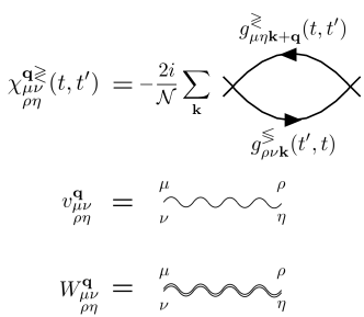
Figure 1: Index-convention for the polarization $\chi$ and for the bare $v$ and screened $W$ Coulomb repulsion.

In order to calculate the RPA screened interaction in the NEQ-EI phase we need to evaluate the irreducible retarded polarization

$$\chi^{{\mathbf{q}}R}_{\vbox{\Let@\restore@math@cr\default@tag\halign{\hfil$\m@th\scriptstyle#$&$\m@th\scriptstyle{}#$\cr&\nu\mu\\ &\eta\rho\crcr}}}(t,t^{\prime}) = \theta(t-t^{\prime})[\chi^{{\mathbf{q}}>}_{\vbox{\Let@\restore@math@cr\default@tag\halign{\hfil$\m@th\scriptstyle#$&$\m@th\scriptstyle{}#$\cr&\nu\mu\\ &\eta\rho\crcr}}}(t,t^{\prime})-\chi^{{\mathbf{q}}<}_{\vbox{\Let@\restore@math@cr\default@tag\halign{\hfil$\m@th\scriptstyle#$&$\m@th\scriptstyle{}#$\cr&\nu\mu\\ &\eta\rho\crcr}}}(t,t^{\prime})],$$ (19)

where the greater and lesser component are shown in Fig. 1 and read

$$\chi^{{\mathbf{q}}\gtrless}_{\vbox{\Let@\restore@math@cr\default@tag\halign{\hfil$\m@th\scriptstyle#$&$\m@th\scriptstyle{}#$\cr&\nu\mu\\ &\eta\rho\crcr}}}(t,t^{\prime}) \equiv -\frac{i}{\mbox{$\mathcal{N}$}}\sum_{{\mathbf{k}}\sigma}g_{\mu\eta{\mathbf{k}}+{\mathbf{q}}\sigma\sigma}^{\gtrless}(t,t^{\prime})g_{\rho\nu{\mathbf{k}}\sigma\sigma}^{\lessgtr}(t^{\prime},t)$$ (22)

$$= -\frac{2i}{\mbox{$\mathcal{N}$}}\sum_{{\mathbf{k}}}g_{\mu\eta{\mathbf{k}}+{\mathbf{q}}}^{\gtrless}(t,t^{\prime})g_{\rho\nu{\mathbf{k}}}^{\lessgtr}(t^{\prime},t).$$ (23)

The lesser and greater Green’s function $g_{{\mathbf{k}}\sigma\sigma^{\prime}}^{\lessgtr}(t,t^{\prime})\equiv\delta_{\sigma\sigma^{\prime}}g_{{\mathbf{k}}}^{\lessgtr}(t,t^{\prime})$ can be conveniently written as

$$g_{\alpha\beta{\mathbf{k}}}^{\gtrless}(t,t^{\prime})=\mp i\varphi^{\pm}_{\alpha{\mathbf{k}}}\varphi^{\pm}_{\beta{\mathbf{k}}}e^{-ie^{\pm}_{{\mathbf{k}}}(t-t^{\prime})}e^{i\frac{\delta\mu}{2}(S_{\alpha}t-S_{\beta}t^{\prime})},$$ (24)

with $S_{v}=1$ and $S_{c}=-1$. In the ground-state band-insulating phase ($\delta\mu=0$) the anomalous off-diagonal components vanish and the Green’s function depends on the time difference $(t-t^{\prime})$ only. In the NEQ-EI phase instead the off-diagnal elements are nonzero (symmetry broken phase) and hence the Green’s function is no longer invariant under time translations. Taking into account the explicit form of the Green’s function we see that $\chi^{{\mathbf{q}}\gtrless}_{\vbox{\Let@\restore@math@cr\default@tag\halign{\hfil$\m@th\scriptstyle#$&$\m@th\scriptstyle{}#$\cr&\mu\nu\\ &\rho\eta\crcr}}}(t,t^{\prime})$ reads

$$\chi^{{\mathbf{q}}\gtrless}_{\vbox{\Let@\restore@math@cr\default@tag\halign{\hfil$\m@th\scriptstyle#$&$\m@th\scriptstyle{}#$\cr&\nu\mu\\ &\eta\rho\crcr}}}(t,t^{\prime}) =-\frac{2i}{\mbox{$\mathcal{N}$}}\sum_{{\mathbf{k}}}\varphi^{\pm}_{\mu{\mathbf{k}}+{\mathbf{q}}}\varphi^{\pm}_{\eta{\mathbf{k}}+{\mathbf{q}}}\varphi^{\mp}_{\rho{\mathbf{k}}}\varphi^{\mp}_{\nu{\mathbf{k}}}$$ (27)

$$\times e^{-i(e^{\pm}_{{\mathbf{k}}+{\mathbf{q}}}-e^{\mp}_{{\mathbf{k}}})(t-t^{\prime})}e^{i\frac{\delta\mu}{2}[(S_{\mu}-S_{\nu})t-(S_{\eta}-S_{\rho})t^{\prime}]}.$$ (28)

The NEQ polarization has a complex time dependence and therefore the RPA screened interaction is, in general, not invariant under time-translations. For a bare interaction $v^{{\mathbf{q}}}_{\vbox{\Let@\restore@math@cr\default@tag\halign{\hfil$\m@th\scriptstyle#$&$\m@th\scriptstyle{}#$\cr&\mu\nu\\ &\eta\rho\crcr}}}(t,t^{\prime})=\delta(t-t^{\prime})v^{{\mathbf{q}}}_{\vbox{\Let@\restore@math@cr\default@tag\halign{\hfil$\m@th\scriptstyle#$&$\m@th\scriptstyle{}#$\cr&\mu\nu\\ &\eta\rho\crcr}}}$ and screened interaction $W^{{\mathbf{q}}}_{\vbox{\Let@\restore@math@cr\default@tag\halign{\hfil$\m@th\scriptstyle#$&$\m@th\scriptstyle{}#$\cr&\mu\nu\\ &\eta\rho\crcr}}}(t,t^{\prime})$ as in Fig. 1, the RPA equation reads

$$W^{{\mathbf{q}}}_{\vbox{\Let@\restore@math@cr\default@tag\halign{\hfil$\m@th\scriptstyle#$&$\m@th\scriptstyle{}#$\cr&\mu\nu\\ &\eta\rho\crcr}}}(t,t^{\prime})=\delta(t-t^{\prime})v^{{\mathbf{q}}}_{\vbox{\Let@\restore@math@cr\default@tag\halign{\hfil$\m@th\scriptstyle#$&$\m@th\scriptstyle{}#$\cr&\mu\nu\\ &\eta\rho\crcr}}}+\sum_{\vbox{\Let@\restore@math@cr\default@tag\halign{\hfil$\m@th\scriptstyle#$&$\m@th\scriptstyle{}#$\cr&\alpha\beta\\ &\gamma\delta\crcr}}}\int\!\!d\bar{t}\,v^{{\mathbf{q}}}_{\vbox{\Let@\restore@math@cr\default@tag\halign{\hfil$\m@th\scriptstyle#$&$\m@th\scriptstyle{}#$\cr&\mu\nu\\ &\beta\alpha\crcr}}}\chi^{{\mathbf{q}}R}_{\vbox{\Let@\restore@math@cr\default@tag\halign{\hfil$\m@th\scriptstyle#$&$\m@th\scriptstyle{}#$\cr&\beta\alpha\\ &\gamma\delta\crcr}}}(t,\bar{t})W^{{\mathbf{q}}}_{\vbox{\Let@\restore@math@cr\default@tag\halign{\hfil$\m@th\scriptstyle#$&$\m@th\scriptstyle{}#$\cr&\gamma\delta\\ &\eta\rho\crcr}}}(\bar{t},t).$$ (29)

In our case, however, the bare interaction couples only pairs of indices belonging to the same band, i.e., $v^{{\mathbf{q}}}_{\vbox{\Let@\restore@math@cr\default@tag\halign{\hfil$\m@th\scriptstyle#$&$\m@th\scriptstyle{}#$\cr&\mu\nu\\ &\rho\eta\crcr}}}=\delta_{\mu\nu}\delta_{\rho\eta}U^{{\mathbf{q}}}_{\mu\rho}$. Consequently, Eq. (29) is solved by $W^{{\mathbf{q}}}_{\vbox{\Let@\restore@math@cr\default@tag\halign{\hfil$\m@th\scriptstyle#$&$\m@th\scriptstyle{}#$\cr&\mu\nu\\ &\rho\eta\crcr}}}=\delta_{\mu\nu}\delta_{\rho\eta}W^{{\mathbf{q}}}_{\mu\rho}$ with

$$W^{{\mathbf{q}}}_{\mu\rho}(t,t^{\prime})=U^{{\mathbf{q}}}_{\mu\rho}\delta(t-t^{\prime})+\sum_{\beta\gamma}U^{{\mathbf{q}}}_{\mu\beta}\int d\bar{t}\chi^{{\mathbf{q}}R}_{\vbox{\Let@\restore@math@cr\default@tag\halign{\hfil$\m@th\scriptstyle#$&$\m@th\scriptstyle{}#$\cr&\beta\beta\\ &\gamma\gamma\crcr}}}(t,\bar{t})W^{{\mathbf{q}}}_{\gamma\rho}(\bar{t},t).$$ (30)

Taking into account Eq. (28) we see that $\chi^{{\mathbf{q}}R}_{\vbox{\Let@\restore@math@cr\default@tag\halign{\hfil$\m@th\scriptstyle#$&$\m@th\scriptstyle{}#$\cr&\beta\beta\\ &\gamma\gamma\crcr}}}(t,\bar{t})$, defined in Eq. (19), depends only on $t-\bar{t}$. Its explicit form is given below

$$\chi^{{\mathbf{q}}R}_{\vbox{\Let@\restore@math@cr\default@tag\halign{\hfil$\m@th\scriptstyle#$&$\m@th\scriptstyle{}#$\cr&\beta\beta\\ &\gamma\gamma\crcr}}}(t,\bar{t}) =-i\theta(t-t^{\prime})\frac{2}{\mbox{$\mathcal{N}$}}$$ (33)

$$\times\sum_{{\mathbf{k}}}\left[\varphi^{+}_{\beta{\mathbf{k}}+{\mathbf{q}}}\varphi^{+}_{\gamma{\mathbf{k}}+{\mathbf{q}}}\varphi^{-}_{\gamma{\mathbf{k}}}\varphi^{-}_{\beta{\mathbf{k}}}e^{-i(e^{+}_{{\mathbf{k}}+{\mathbf{q}}}-e^{-}_{{\mathbf{k}}})(t-\bar{t})}\right.$$

$$\left.\varphi^{-}_{\beta{\mathbf{k}}+{\mathbf{q}}}\varphi^{-}_{\gamma{\mathbf{k}}+{\mathbf{q}}}\varphi^{+}_{\gamma{\mathbf{k}}}\varphi^{+}_{\beta{\mathbf{k}}}e^{-i(e^{-}_{{\mathbf{k}}+{\mathbf{q}}}-e^{+}_{{\mathbf{k}}})(t-\bar{t})}\right].$$ (34)

This has an important consequence since the Fourier transform of Eq. (30) becomes simply

$$W^{{\mathbf{q}}}_{\mu\rho}(\omega)=U^{{\mathbf{q}}}_{\mu\rho}+\sum_{\beta\gamma}U^{{\mathbf{q}}}_{\mu\beta}\chi^{{\mathbf{q}}R}_{\vbox{\Let@\restore@math@cr\default@tag\halign{\hfil$\m@th\scriptstyle#$&$\m@th\scriptstyle{}#$\cr&\beta\beta\\ &\gamma\gamma\crcr}}}(\omega)W^{{\mathbf{q}}}_{\gamma\rho}(\omega),$$ (35)

where

$$\chi^{{\mathbf{q}}R}_{\vbox{\Let@\restore@math@cr\default@tag\halign{\hfil$\m@th\scriptstyle#$&$\m@th\scriptstyle{}#$\cr&\alpha\alpha\\ &\beta\beta\crcr}}}(\omega)=\frac{2}{\mbox{$\mathcal{N}$}}\sum_{{\mathbf{k}}}\left[\frac{\varphi^{+}_{\alpha{\mathbf{k}}+{\mathbf{q}}}\varphi^{+}_{\beta{\mathbf{k}}+{\mathbf{q}}}\varphi^{-}_{\alpha{\mathbf{k}}}\varphi^{-}_{\beta{\mathbf{k}}}}{\omega-(e^{+}_{{\mathbf{k}}+{\mathbf{q}}}-e^{-}_{{\mathbf{k}}})+i\eta}\right.$$ (38)

$$\left.-\frac{\varphi^{-}_{\alpha{\mathbf{k}}+{\mathbf{q}}}\varphi^{-}_{\beta{\mathbf{k}}+{\mathbf{q}}}\varphi^{+}_{\alpha{\mathbf{k}}}\varphi^{+}_{\beta{\mathbf{k}}}}{\omega-(e^{-}_{{\mathbf{k}}+{\mathbf{q}}}-e^{+}_{{\mathbf{k}}})+i\eta}\right].$$ (39)

More analytic manipulations are possible by taking the inter-band repulsion identical to the intra-band repulsion, i.e., $U^{{\mathbf{q}}}_{\mu\nu}=U^{{\mathbf{q}}}$ (in this case the Hartree contributions in $\delta V^{\rm HF}_{{\mathbf{k}}}$ cancel out). In fact, Eq. (35) is then solved by $W^{{\mathbf{q}}}_{\mu\rho}(\omega)=W^{{\mathbf{q}}}_{\rm exciton}(\omega)$ with exciton screening

$$W^{{\mathbf{q}}}_{\mathrm{exciton}}(\omega)=\frac{U^{{\mathbf{q}}}}{1-U^{{\mathbf{q}}}\left[\chi^{{\mathbf{q}}R}_{\vbox{\Let@\restore@math@cr\default@tag\halign{\hfil$\m@th\scriptstyle#$&$\m@th\scriptstyle{}#$\cr&vv\\ &vv\crcr}}}(\omega)+\chi^{{\mathbf{q}}R}_{\vbox{\Let@\restore@math@cr\default@tag\halign{\hfil$\m@th\scriptstyle#$&$\m@th\scriptstyle{}#$\cr&cc\\ &cc\crcr}}}(\omega)+2\chi^{{\mathbf{q}}R}_{\vbox{\Let@\restore@math@cr\default@tag\halign{\hfil$\m@th\scriptstyle#$&$\m@th\scriptstyle{}#$\cr&vv\\ &cc\crcr}}}(\omega)\right]},$$ (40)

where we have used the symmetry property $\chi^{{\mathbf{q}}R}_{\vbox{\Let@\restore@math@cr\default@tag\halign{\hfil$\m@th\scriptstyle#$&$\m@th\scriptstyle{}#$\cr&vv\\ &cc\crcr}}}=\chi^{{\mathbf{q}}R}_{\vbox{\Let@\restore@math@cr\default@tag\halign{\hfil$\m@th\scriptstyle#$&$\m@th\scriptstyle{}#$\cr&cc\\ &vv\crcr}}}$. In the following we consider only the static screening and calculate all quantities at $\omega=0$: $W^{{\mathbf{q}}}_{\mathrm{exciton}}(0)\equiv W^{{\mathbf{q}}}_{\mathrm{exciton}}$ and $\chi^{{\mathbf{q}}R}(0)\equiv\chi^{{\mathbf{q}}R}$.

It is worth comparing the screening in the NEQ-EI phase with the screening of the unbroken symmetry phase ($\Delta=0$). In this phase the system can either be a band insulator or a normal metal, depending on the value of $\delta\mu$. In both cases the anomalous components of the Green’s function vanish, hence $\chi^{{\mathbf{q}}R}_{\vbox{\Let@\restore@math@cr\default@tag\halign{\hfil$\m@th\scriptstyle#$&$\m@th\scriptstyle{}#$\cr&vv\\ &cc\crcr}}}=0$, and the screened interaction reduces to

$$W^{{\mathbf{q}}}_{\mathrm{plasma}}=\frac{U^{{\mathbf{q}}}}{1-U^{{\mathbf{q}}}(\chi^{{\mathbf{q}}R}_{\vbox{\Let@\restore@math@cr\default@tag\halign{\hfil$\m@th\scriptstyle#$&$\m@th\scriptstyle{}#$\cr&vv\\ &vv\crcr}}}+\chi^{{\mathbf{q}}R}_{\vbox{\Let@\restore@math@cr\default@tag\halign{\hfil$\m@th\scriptstyle#$&$\m@th\scriptstyle{}#$\cr&cc\\ &cc\crcr}}})},$$ (41)

where

$$\chi^{{\mathbf{q}}R}_{\vbox{\Let@\restore@math@cr\default@tag\halign{\hfil$\m@th\scriptstyle#$&$\m@th\scriptstyle{}#$\cr&\alpha\alpha\\ &\alpha\alpha\crcr}}}=\frac{2}{\mbox{$\mathcal{N}$}}\sum_{{\mathbf{k}}}\frac{\bar{f}_{\alpha{\mathbf{k}}+{\mathbf{q}}}f_{\alpha{\mathbf{k}}}-f_{\alpha{\mathbf{k}}+{\mathbf{q}}}\bar{f}_{\alpha{\mathbf{k}}}}{-\epsilon^{\rm HF}_{\alpha{\mathbf{k}}+{\mathbf{q}}}+\epsilon^{\rm HF}_{\alpha{\mathbf{k}}}+i\eta}$$ (42)

is the Lindhard function of a noninteracting gas made of conduction electrons up to energy $\mu_{c}$ and valence electrons up to energy $\mu_{v}$ (we remind that $f_{\alpha{\mathbf{k}}}=0$ for $\epsilon^{\rm HF}_{\alpha{\mathbf{k}}}>\mu_{\alpha}$ and unity otherwise). Clearly Eq. (42) is non zero only in the metallic case and we recover the plasma screening of metals for which the interaction is maximally screened at ${\mathbf{q}}=\mathbf{0}$. Indeed the static polarization of an electron gas is real and negative, reaching its minimum value for ${\mathbf{q}}\to\mathbf{0}$. We also observe that the plasma screening correctly vanishes in the band insulating phase ($0<\delta\mu<\epsilon_{\rm x}$) since $\chi^{{\mathbf{q}}R}_{\vbox{\Let@\restore@math@cr\default@tag\halign{\hfil$\m@th\scriptstyle#$&$\m@th\scriptstyle{}#$\cr&vv\\ &vv\crcr}}}=\chi^{{\mathbf{q}}R}_{\vbox{\Let@\restore@math@cr\default@tag\halign{\hfil$\m@th\scriptstyle#$&$\m@th\scriptstyle{}#$\cr&cc\\ &cc\crcr}}}=0$, leading to $W^{{\mathbf{q}}}_{\mathrm{plasma}}=U^{{\mathbf{q}}}$.

The exciton screening in Eq. (40) is qualitatively and quantitatively different. Since we have chosen real and normalized eigenvectors we always have

$$\varphi^{-}_{c{\mathbf{k}}}=\varphi^{+}_{v{\mathbf{k}}}\quad,\quad\varphi^{+}_{c{\mathbf{k}}}=-\varphi^{-}_{v{\mathbf{k}}},$$ (43)

and therefore the long-wavelenght limit ${\mathbf{q}}\to\mathbf{0}$ of Eq. (39) yields

$$\chi^{R{\mathbf{q}}=\mathbf{0}}_{\vbox{\Let@\restore@math@cr\default@tag\halign{\hfil$\m@th\scriptstyle#$&$\m@th\scriptstyle{}#$\cr&vv\\ &vv\crcr}}}=\chi^{R{\mathbf{q}}=\mathbf{0}}_{\vbox{\Let@\restore@math@cr\default@tag\halign{\hfil$\m@th\scriptstyle#$&$\m@th\scriptstyle{}#$\cr&cc\\ &cc\crcr}}}=-\chi^{R{\mathbf{q}}=\mathbf{0}}_{\vbox{\Let@\restore@math@cr\default@tag\halign{\hfil$\m@th\scriptstyle#$&$\m@th\scriptstyle{}#$\cr&vv\\ &cc\crcr}}}.$$ (44)

Consequently the denominator of the screened interaction in Eq. (40) is unity and

$$W^{{\mathbf{q}}=\mathbf{0}}_{\mathrm{exciton}}=U^{{\mathbf{q}}=\mathbf{0}}.$$ (45)

This is a remarkable property conveying a clear physical message: in the NEQ-EI phase the long-wavelength limit of the interaction is not screened. With hindsight we may say that in a NEQ-EI electrons and holes pair to form bound excitons which behave like microscopic electric dipoles; hence their screening efficiency at long distances is correctly negligible. Notice that starting from the NEQ-EI phase and reducing $\delta\mu$ it is not possible to recover the plasmon screening of the unbroken symmetry phase since the limit $\delta\mu\to 0$ and $\delta{\mathbf{q}}\to 0$ do not commute, see also Fig. 4. We also observe that the perfect cancellation in Eq. (44) is a consequence of the assumptions made, i.e., two-band model and a Coulomb tensor independent of the band indices. However this analytic result points to a strong cancellation between the anomalous and normal polarization in more refined descriptions, and hence to a considerably reduced screening in the NEQ-EI phase as compared to that of quasi-free carriers.

IV Hartree plus Screened Exchange NEQ-EI

In this Section we describe the self-consistent procedure to study the NEQ-EI phase within the HSEX approximation. The equation to be solved is the same as the HF one, see Eq. (8), except that we have to replace $U_{{\mathbf{q}}}\to W^{{\mathbf{q}}}_{\mathrm{exciton}}$ in the exchange terms, i.e.

$$\left(\begin{array}[]{cc}\epsilon^{\rm HF}_{v{\mathbf{k}}}+\frac{1}{\mbox{$\mathcal{N}$}}\sum_{{\mathbf{q}}}W^{{\mathbf{k}}-{\mathbf{q}}}_{\mathrm{exciton}}|\varphi^{-}_{c{\mathbf{q}}}|^{2}-\frac{\delta\mu}{2}&-\frac{1}{\mbox{$\mathcal{N}$}}\sum_{{\mathbf{q}}}W^{{\mathbf{k}}-{\mathbf{q}}}_{\mathrm{exciton}}\varphi^{-}_{c{\mathbf{q}}}\varphi^{-}_{v{\mathbf{q}}}\\ -\frac{1}{\mbox{$\mathcal{N}$}}\sum_{{\mathbf{q}}}W^{{\mathbf{k}}-{\mathbf{q}}}_{\mathrm{exciton}}\varphi^{-}_{c{\mathbf{q}}}\varphi^{-}_{v{\mathbf{q}}}&\epsilon^{\rm HF}_{c{\mathbf{k}}}-\frac{1}{\mbox{$\mathcal{N}$}}\sum_{{\mathbf{q}}}W^{{\mathbf{k}}-{\mathbf{q}}}_{\mathrm{exciton}}|\varphi^{-}_{c{\mathbf{q}}}|^{2}+\frac{\delta\mu}{2}\\ \end{array}\right)\left(\begin{array}[]{c}\varphi^{\lambda}_{v{\mathbf{k}}}\\ \varphi^{\lambda}_{c{\mathbf{k}}}\end{array}\right)=(e^{\lambda}_{{\mathbf{k}}}+\mu)\left(\begin{array}[]{c}\varphi^{\lambda}_{v{\mathbf{k}}}\\ \varphi^{\lambda}_{c{\mathbf{k}}}\end{array}\right).$$ (46)

A working algorithm to solve the problem is proposed below:

1. Solve the HF problem, i.e., solve self-cosistently Eq. (8);
   

2. Use $\varphi^{\lambda}_{\mu{\mathbf{q}}}$ and $e^{\lambda}_{{\mathbf{q}}}$ to calculate $W^{{\mathbf{q}}}_{\mathrm{exciton}}$ in Eq. (40);
   

3. Use $W^{{\mathbf{q}}}_{\mathrm{exciton}}$ to solve self-cosistently the HSEX problem in Eq. (46);
   

4. Use the new $\varphi^{\lambda}_{\mu{\mathbf{q}}}$ and $e^{\lambda}_{{\mathbf{q}}}$ to update $W^{{\mathbf{q}}}_{\mathrm{exciton}}$ in Eq. (40);

5. Repeat steps 3 and 4 until convergence.

In the next Section we discuss the results of the above numerical scheme for a 2-dimensional (2D) semiconductor with parabolic band dispersion.

V Two-Dimensional model for $\mathrm{MoS}_{2}$

We consider a $\mathrm{MoS}_{2}$ monolayer and approximate the valence and conduction bands close to the K and K’ valleys with the parabolic dispersion $\epsilon^{\rm HF}_{v{\mathbf{k}}}=-\frac{k^{2}}{2m}-\frac{\epsilon_{g}}{2}$ and $\epsilon^{\rm HF}_{c{\mathbf{k}}}=\frac{k^{2}}{2m}+\frac{\epsilon_{g}}{2}$ respectively, with $k=|{\mathbf{k}}|$. We can easily determine the value of the chemical potential $\mu$ to fulfill the charge neutrality condition in Eq. (10). Since $\epsilon^{\rm HF}_{c{\mathbf{k}}}=-\epsilon^{\rm HF}_{v{\mathbf{k}}}$ and $U^{{\mathbf{q}}}_{\mu\nu}=U^{{\mathbf{q}}}$ we have $\mu=0$ for all $\delta\mu$. According to Ref. excscr4 an accurate parametrization of the Coulomb interaction $U^{{\mathbf{q}}}$ for particles in one of the two valleys is

$$U^{{\mathbf{q}}}=\frac{V^{{\mathbf{q}}}}{\epsilon_{{\mathbf{q}}}},$$ (47)

where

$$V^{{\mathbf{q}}} = \frac{2\pi}{q(1+\gamma q+\delta q^{2})},$$

$$\epsilon_{{\mathbf{q}}} = \epsilon^{\infty}_{{\mathbf{q}}}\frac{1-\beta_{1{\mathbf{q}}}\beta_{2{\mathbf{q}}}e^{-2hq}}{1+(\beta_{1{\mathbf{q}}}+\beta_{2{\mathbf{q}}})e^{-hq}+\beta_{1{\mathbf{q}}}\beta_{2{\mathbf{q}}}e^{-2hq}},$$

$$\beta_{i{\mathbf{q}}} = \frac{\epsilon^{\infty}_{{\mathbf{q}}}-\epsilon_{\mathrm{sub,i}}}{\epsilon^{\infty}_{{\mathbf{q}}}+\epsilon_{\mathrm{sub,i}}},$$

$$\epsilon^{\infty}_{{\mathbf{q}}} = g+\frac{a+q^{2}}{\frac{a\sin(qc)}{qbc}+q^{2}}.$$ (48)

The dielectric constant $\epsilon^{\infty}_{{\mathbf{q}}}$ accounts for the background screening originating from the electronic bands which are neglected, while $\epsilon_{\mathrm{sub,i}}$ is the dielectric constant of a possible substrate ($i=1$) or superstrate ($i=2$). Realistic parameters to describe a free-standing layer of MoS₂ are $m/m_{e}=0.6$ (where $m_{e}$ is the free electron mass), $\epsilon_{g}=2.72~{}\mathrm{eV}$, $a=2.3~{}\mathring{\mathrm{A}}^{-2}$, $b=17$, $c=5~{}\mathring{\mathrm{A}}$, $h=2.7~{}\mathring{\mathrm{A}}$, $g=5.7$, $\gamma=1.9~{}\mathring{\mathrm{A}}$, $\delta=0.395~{}\mathring{\mathrm{A}}^{2}$, and $\epsilon_{\mathrm{sub,i}}=1$. We have verified that the solution of the Bethe-Salpeter equation with the above parameters provides the lowest excitonic level at $\epsilon_{\mathrm{x}}=2.15~{}\mathrm{eV}$ with corresponding binding energy $\epsilon_{b}=0.57~{}\mathrm{eV}$, in good agreement with the literature plasma1 .

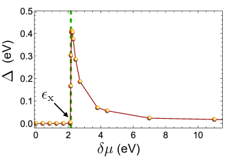
Figure 2: HF phase diagram. Order parameter $\Delta$ defined in Eq. (12) obtained from the self-consitent solution of Eq. (8) for different values of $\delta\mu$. The vertical dashed line indicates the lowest exciton energy $\epsilon_{\mathrm{x}}=2.15~{}\mathrm{eV}$.

V.1 HF phase diagram

In Fig. 2 we show the NEQ-EI phase diagram by displaying the amplitude of the order parameter $\Delta$ defined in Eq. 12 versus $\delta\mu$. As discussed in Ref. neqei11, the order parameter $\Delta$ and the excited density in conduction band $n_{c}=\frac{2}{\mbox{$\mathcal{N}$}}\sum_{{\mathbf{k}}}|\varphi^{-}_{c{\mathbf{k}}}|^{2}$ vanish for $\delta\mu<\epsilon_{\mathrm{x}}$. The transition between the band-insulating and the NEQ-EI phases occurs at the critical value $\delta\mu=\epsilon_{\mathrm{x}}=2.15$ eV. As $\delta\mu$ is increased, $\Delta$ displays a non monotonous behavior characterized by a sudden raise followed by a slow decrease. We checked that $\Delta$ is not discontinuous in $\delta\mu=\epsilon_{\mathrm{x}}$ and that it reaches its maximum value at $\delta\mu\gtrsim 2.22$ eV.

V.2 HSEX phase diagram

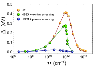
Figure 3: HSEX vs HF phase diagrams. Order parameter $\Delta$ calculated in the HF approximation according to Eq. (8) (yellow circles) and in the HSEX approximation according to Eq. (46) (green circles) as a function of the excited denisty $n$. For comparison we also show $\Delta$ obtained using a plasma screening (blue circles), i.e. by solving Eq. (46) with the replacement $W^{{\mathbf{q}}}_{\mathrm{exciton}}\to W^{{\mathbf{q}}}_{\mathrm{plasma}}$.

In Fig. 3 we compare the HF phase diagram with the HSEX one. For this comparison we have found more instructive to plot the order parameter $\Delta$ versus the excited density per unit cell, i.e., $n=2n_{c}/A$, where $A=8.8\times 10^{-16}~{}\mathrm{cm}^{2}$ is the area of the unit cell of a $\mathrm{MoS}_{2}$ monolayer. The extra factor $2$ accounts for the fact that the total excited carriers are equally distributed among the $\mathrm{K}$ and $\mathrm{K}^{\prime}$ valleys.

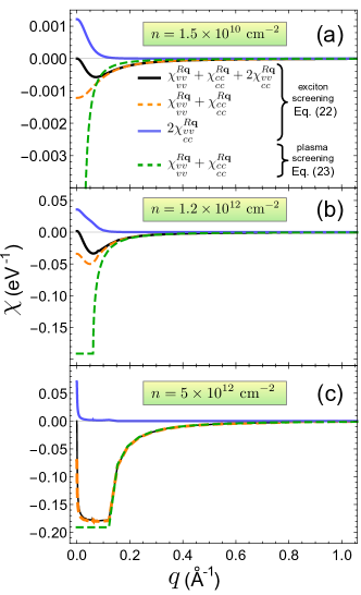
Figure 4: The relevant components of the polarization $\chi$ for different excited densities $n$ and for different screening approximations. In the case of excitonic screening the total $\chi$ (black solid curve) entering in Eq. (40) has both normal (orange dashed curve) and anomalous (blue solid curve) components. In the case of plasma screening, instead, the total $\chi$ entering in Eq. (41) coincides with its normal component (green dashed curve).

In addition to the full HSEX solution we also show the outcome of the self-consistent solution of Eq. (46) with the replacement $W^{{\mathbf{q}}}_{\mathrm{exciton}}\to W^{{\mathbf{q}}}_{\mathrm{plasma}}$ in Eq. (41). This comparison is useful to highlight the importance of screening the interaction with a polarization originating from an exciton superfluid rather than from a plasma of free carries. For parabolic 2D bands the polarization in Eq. (42) has an analytic expression vignale :

$$\chi^{R{\mathbf{q}}}_{\vbox{\Let@\restore@math@cr\default@tag\halign{\hfil$\m@th\scriptstyle#$&$\m@th\scriptstyle{}#$\cr&vv\\ &vv\crcr}}}=\chi^{R{\mathbf{q}}}_{\vbox{\Let@\restore@math@cr\default@tag\halign{\hfil$\m@th\scriptstyle#$&$\m@th\scriptstyle{}#$\cr&cc\\ &cc\crcr}}}=-\frac{m}{\pi}\left[1-\theta(q-2k_{\mathrm{F}})\sqrt{1-4k_{\mathrm{F}}^{2}/q^{2}}\right],$$ (49)

where $k_{\mathrm{F}}=\sqrt{2\pi n_{c}}$.

Figure 3 clearly shows that the NEQ-EI phase survives in a large portion of the phase diagram provided that the proper screened interaction is considered. In particular for low and moderate excited densities $n\lesssim 10^{11}\mathrm{cm}^{-2}$ the screening efficiency of the exciton superfluid is scarce and the HF and HSEX results are quite similar. In this regime, however, the plasma screening is already strong and the corresponding order parameter is highly suppressed. The dramatic impact of different screenings on the phase diagram can be better understood with the help of Fig. 4a. For low excited density $n$ the excitonic polarization is much smaller than the plasma one. In particular the plasma $\chi$ (green dashed) is large and independent on $n$ for small ${\mathbf{q}}$ (its value at ${\mathbf{q}}=\mathbf{0}$ is $-m/\pi\approx-0.19~{}\mathrm{eV}^{-1}$) whereas the excitonic $\chi$ (black solid) is almost vanishing due to the cancellation between off-diagonal (blue solid) and diagonal (orange dashed) components, see discussion in Section III. For higher densities the screening of the exciton superfluid becomes more efficient although the normal and anomalous components of $\chi$ still partially cancel at low momenta ${\mathbf{q}}$, see Fig. 4b. As a result the HSEX order parameter is somewhat reduced and it reaches its maximum value concomitantly with the HF order parameter at density $n_{\mathrm{max}}\approx 10^{12}\mathrm{cm}^{-2}$. For this density the screening is responsible for a 25% reduction of the HF order parameter. At the same density the plasma screening does instead suppress the order parameter by two orders of magnitude. For $n>n_{\mathrm{max}}$ the HSEX results depart significantly from the HF values, see Fig. 3. In particular the HF order parameter decreases smoothly whereas in HSEX $n=n_{\mathrm{max}}$ is, de facto, a critical value beyond which the NEQ-EI phase breaks down. We refer to this density-driven transition as coherent excitonic Mott transition. This should not be confused with the well-known excitonic Mott transition mott1 ; mott2 ; mott3 ; mott4 which, instead, refers to the incoherent regime.

The observed behavior can again be understood by inspecting the polarization, see Fig. 4c. At densities $n\gtrsim n_{\mathrm{max}}$ the excitons start melting and the screening efficiency changes, becoming similar to the plasma efficiency. In fact, although $\chi$ still vanishes at ${\mathbf{q}}=\mathbf{0}$ (this is an exact property for any $\Delta\neq 0$) the aforementioned cancellation occurs only in a very tiny region around ${\mathbf{q}}=\mathbf{0}$.

The phase diagram in Fig. 3 provides a reliable description of MoS₂ up to $\delta\mu\lesssim 3.2$ eV. Indeed, in this range the chemical potentials $\mu_{c}$/$\mu_{v}$ lie about $0.2$ eV above/below the band miminum/maximum, and the parabolic approximation for the band dispersion is still accurate exc1 . The value $\delta\mu=3.2$ eV corresponds to $n\sim 5\times 10^{12}\mathrm{cm}^{-2}$, thus covering the whole range of our HSEX calculations.

VI Summary and Conclusions

We presented a microscopic approach to address the stability of the exciton superfluid created by a resonant pump against an increasing density in the conduction bands. Using different chemical potential for valence and conduction electrons self-consistency naturally leads to the non-stationary NEQ-EI state neqei11 . Our theory improves over previous studies in the RPA screened electron-hole interaction which we here calculate using the polarization of the proper state of matter, i.e., the exciton superfluid. We find that the screening does not affect the long-wavelength component of the interaction due to the neutral nature of the excitons. This property origins from a subtle cancellation between a plasma-like contribution and an anomalous one. Inclusion of the proper screening in a self-consistent HSEX calculation indicates that the NEQ-EI phase is very robust, and can survive up to densities typically excited in pump-probe experiments. Numerical calculations in MoS₂ monolayers show that the HF (i.e. unscreened) phase diagram is very similar to the HSEX phase diagram up to a critical density $n_{\mathrm{max}}\sim 10^{12}\mathrm{cm}^{-2}$, where the excitonic order parameter reaches its maximum value. However, by further increasing the density in the conduction bands excitons start melting consistently with an increase in the screening efficiency. When $n\sim n_{\mathrm{max}}$, the HSEX approach predicts the occurrence of a coherent excitonic Mott transition. We do not expect that the observed sharpness is universal as other scenarios, like phase coexistence, are possible capone .

Our results are relevant also in the light of future first-principles studies of the NEQ-EI phase occurring in normal semiconductors. Indeed we have provided evidence that at least for small and moderate excited densities the update of the screened interaction in the excited state is presumably not necessary, thus rendering the NEQ-EI mean-field problem easily implementable in most of the already existing ab initio codes.

Acknowledgements G.S. and E.P. acknowledge funding through the RISE Co-ExAN (Grant No. GA644076) and the INFN17-nemesys project. G.S., and E.P. acknowledge funding through the MIUR PRIN (Grant No. 20173B72NB). A.M., and E.P. acknowledge funding received from the European Union projects: MaX Materials design at the eXascale H2020-EINFRA-2015-1, Grant agreement n. 676598, and H2020-INFRAEDI-2018-2020/H2020-INFRAEDI-2018-1, Grant agreement n. 824143; Nanoscience Foundries and Fine Analysis - Europe H2020-INFRAIA-2014-2015, Grant agreement n. 654360. (Grant Agreement No. 654360). G.S. acknowledges Tor Vergata University for financial support through the Mission Sustainability Project 2DUTOPI.

References

• (1) S. Manzeli, D. Ovchinnikov, D. Pasquier, O. V. Yazyev, and A. Kis, Nat. Rev. Mater. 2, 17033 (2017).
• (2) Q. H. Wang, K. Kalantar-Zadeh, A. Kis, J. N. Coleman, and M. S.Strano, Nat. Nanotechnol. 7, 699 (2012).
• (3) M. Chhowalla, H. S. Shin, G. Eda, L. J. Li, K. P. Loh, and H. Zhang, Nat. Chem. 5, 263 (2013).
• (4) S. Z. Butler, et al., ACS Nano 7, 2898 (2013).
• (5) K. F. Mak and J. Shan, Nat. Photonics 10, 216 (2016).
• (6) D. Y. Qiu, F. H. da Jornada, and S. G. Louie, Phys. Rev. Lett. 111, 216805 (2013).
• (7) K. He, N. Kumar, L. Zhao, Z. Wang, K. F. Mak, H. Zhao, and J. Shan, Phys. Rev. Lett. 113, 026803 (2014).
• (8) G. Wang, A. Chernikov, M. M. Glazov, T. F. Heinz, X.Marie, T. Amand, and B. Urbaszek, Rev. Mod. Phys. 90, 021001 (2018).
• (9) K. F. Mak, K. He, C. Lee, G. H. Lee, J. Hone, T. F. Heinz,and J. Shan, Nat. Mater. 12, 207 (2012).
• (10) J. S. Ross, S. Wu, H. Yu, N. J. Ghimire, A. M. Jones,G. Aivazian, J. Yan, D. G. Mandrus, D. Xiao, W. Yao,and X. Xu, Nat. Commun. 4, 1474 (2013).
• (11) A. Singh, et a.l, Phys. Rev. B 93, 041401(R) (2016).
• (12) G. Plechinger, P. Nagler, J. Kraus, N. Paradiso, C. Strunk,C. Schuller, and T. Korn, Phys. Status Solidi RRL 9, 457 (2015).
• (13) J. Shang, X. Shen, C. Cong, N. Peimyoo, B. Cao, M. Eginligil,and T. Yu, ACS Nano 9, 647 (2015).
• (14) E. J. Sie, A. J. Frenzel, Y.-H. Lee, J. Kong, and N. Gedik, Phys. Rev. B 92, 125417 (2015).
• (15) Y. You, X.-X. Zhang, T. C. Berkelbach, M. S. Hybertsen, D.R. Reichman, and T. F. Heinz, Nat. Phys. 11, 477 (2015).
• (16) X. Liu, T. Galfsky, Z. Sun, F. Xia, E. Lin, Y.-H. Lee, S. Kéna-Cohen, and V. M. Menon, Nat. Photonics 9, 30 (2015).
• (17) S. Dufferwiel et al., Nat. Commun. 6, 8579 (2015).
• (18) L. C. Flatten, Z. He, D. M. Coles, A. A. P. Trichet, A. W. Powell, R. A. Taylor, J. H. Warner, and J. M. Smith, Sci. Rep. 6, 33134 (2016).
• (19) T. Cheiwchanchamnangij and W. R. L. Lambrecht, Phys. Rev. B 85, 205302 (2012).
• (20) A. Ramasubramaniam, Phys. Rev. B 86, 115409 (2012).
• (21) A. Chernikov, et al, Phys. Rev. Lett. 113, 076802 (2014)
• (22) G. Wang, X. Marie, I. Gerber, T. Amand, D. Lagarde, L. Bouet, M. Vidal, A. Balocchi, and B. Urbaszek, Phys. Rev. Lett. 114, 097403 (2015).
• (23) H. Haug and S. W. Koch, Quantum Theory of the Optical and Electronic Properties of Semiconductors, 3rd ed. World Scientific, Singapore, 1994.
• (24) A. Steinhoff, M. Florian, M. Rösner, M. Lorke, T. O. Wehling, C. Gies, and F. Jahnke, 2D Mater. 3, 031006 (2016).
• (25) M. Selig, G. Berghauser, A. Raja, P. Nagler, C. Schuller,T. F. Heinz, T. Korn, A. Chernikov, E. Malic, and A. Knorr, Nat. Commun. 7, 13279 (2016).
• (26) A. Molina-Sánchez, D. Sangalli, L. Wirtz, A. Marini, Nano Lett. 17, 4549 (2017).
• (27) R. Ulbricht, E. Hendry, J. Shan, T. F. Heinz, and M. Bonn, Rev. Mod. Phys. 83, 543 (2011).
• (28) S. W. Koch, M. Kira, G. Khitrova, and H. M. Gibbs, Nat. Mater. 5, 523 (2006).
• (29) E. Perfetto, D. Sangalli, A. Marini, and G. Stefanucci, Phys. Rev. B 94, 245303 (2016).
• (30) A. Chernikov, A. M. van der Zande, H. M. Hill, A. F. Rigosi, A. Velauthapillai, J. Hone, and T. F. Heinz, Phys. Rev. Lett. 115, 126802 (2015).
• (31) P. D. Cunningham, A. T. Hanbicki, K. M. McCreary, and B. T. Jonker, ACS Nano 11, 12601 (2017)
• (32) K. Yao, A. Yan, S. Kahn, A. Suslu, Y. Liang, E. S. Barnard, S. Tongay, A. Zettl, N. J. Borys, and P. J. Schuck, Phys. Rev. Lett. 119, 087401 (2017).
• (33) M. M. Ugeda, A. J. Bradley, S.-F. Shi, F. H. da Jornada, Y.Zhang, D. Y.Qiu, W.Ruan, S.-K.Mo, Z.Hussain, Z.-X.Shen,F. Wang, S. G. Louie, and M. F. Crommie, Nat. Mater. 13,1091 (2014).
• (34) A. Chernikov, C. Ruppert, H. M. Hill, A. F. Rigosi, and T. F. Heinz, Nat. Photonics 9, 466 (2015).
• (35) F. Liu, M. E. Ziffer, K. R. Hansen, J. Wang, and X. Zhu, Phys. Rev. Lett. 122, 246803 (2019).
• (36) M. Dendzik et al., arXiv:2003.12925
• (37) J. Wang, J. Ardelean, Y. Bai, A. Steinhoff, M. Florian, F. Jahnke, X. Xu, M. Kira, J. Hone, X. Y. Zhu, Sci. Adv. 5 eaax0145 (2019).
• (38) W. F. Brinkman and T. M. Rice, Phys. Rev. B 7, 1508 (1973).
• (39) N. F. Mott, Contemporary Physics 14, 401 (1973).
• (40) T. Rice (Academic Press, 1978), vol. 32 of Solid State Physics, pp. 1 – 86.
• (41) N. F. Mott, Proceedings of the Physical Society. Section A 62, 416 (1949).
• (42) A. Steinhoff, M. Rösner, F. Jahnke, T. O. Wehling, and C. Gies, Nano Lett. 14, 3743 (2014).
• (43) L. Meckbach, T. Stroucken, and S. W. Koch, Appl. Phys. Lett. 112, 061104 (2018).
• (44) Y. Liang and L. Yang Phys. Rev. Lett. 114, 063001 (2015).
• (45) G.Röpke and R. Der, Phys. Status Solidi (B) 92, 501 (1979).
• (46) G. Röpke, T. Seifert, and K. Kilimann, Ann. Phys. N.Y. 38, 381 (1981).
• (47) H. Stolz. and R. Zimmerman, Phys. Stat. Sol. (b) 124, 201 (1984).
• (48) A. Steinhoff, M. Florian, M. Rosner, G. Schonhoff, T. O. Wehling, and F. Jahnke, Nat. Commun. 8, 1166 (2017).
• (49) T. Östreichand, and K. Schönhammer, Zeitschrift für, Physik B Condensed Matter 91, 189 (1993).
• (50) K. Hannewald, S. Glutsch, and F. Bechstedt, Journal of Physics: Condensed Matter 13, 275 (2000).
• (51) E. Perfetto, D. Sangalli, A. Marini, and G. Stefanucci, Phys.Rev. Mater. 3,124601 (2019).
• (52) Y. Murakami, M. Schüler, S. Takayoshi, and P. Werner, Phys. Rev. B 101, 035203 (2020).
• (53) E. Perfetto, S. Bianchi and G. Stefanucci, Phys. Rev. B 101, 041201(R) (2020).
• (54) E. Perfetto, and G. Stefanucci, arXiv:2001.08921
• (55) C. Triola, A. Pertsova, R. S. Markiewicz, and A. V. Balatsky, Phys. Rev. B 95, 205410 (2017)
• (56) A. Pertsova and A. V. Balatsky, Phys. Rev. B 97, 075109 (2018).
• (57) R. Hanai, P. B. Littlewood, and Y. Ohashi, Journal of Low Temperature Physics 183, 127 (2016).
• (58) R. Hanai, P. B. Littlewood, and Y. Ohashi, Phys. Rev. B 96, 125206 (2017).
• (59) R. Hanai, P. B. Littlewood, and Y. Ohashi, Phys. Rev. B 97, 245302 (2018).
• (60) K. W. Becker, H. Fehske, and V.-N. Phan, Phys. Rev. B 99, 035304 (2019).
• (61) M. Yamaguchi, K. Kamide, T. Ogawa, and Y. Yamamoto, New Journal of Physics 14, 065001 (2012).
• (62) M. Yamaguchi, K. Kamide, R. Nii, T. Ogawa, and Y. Yamamoto, Phys. Rev. Lett. 111, 026404 (2013).
• (63) Y. Murotani ,C. Kim, H. Akiyama,L. N. Pfeiffer, K. W. West, and R. Shimano, Phys. Rev. Lett. 123, 197401 (2019).
• (64) J. M. Blatt, K. W. Boöer, and W. Brandt, Phys. Rev. 126, 1691 (1962).
• (65) L. V. Keldysh and Y. U. Kopaev, Fiz. Tverd. Tela. 6, 2791 (1964) [Sov. Phys. Solid State 6, 2219 (1965)].
• (66) A. N. Kozlov and L. A. Maksimov, J. Exptl. Theor. Phys. (U.S.S.R.) 48, 1184 (1965) [JETP 21, 790 (1965)].
• (67) D. Jérome, T. M. Rice, and W. Kohn, Phys. Rev. 158, 462 (1967).
• (68) B. Halperin and T. Rice, Solid State Phys. 21, 115 (1968).
• (69) L. V. Keldysh and A. N. Kozlov, Zh. Eksp. Teor. Fiz. 54, 978 (1968) [JETP 27, 521 (1968)].
• (70) C. Comte and P. Noziéres, J. Phys. (France) 43, 1069 (1982).
• (71) C. Comte and P. Noziéres, J. Phys. (France) 43, 1083 (1982).
• (72) A. Mazloom and S. H. Abedinpour, Phys. Rev. B 98, 014513 (2018).
• (73) Yu. E. Lozovik, S. L. Ogarkov, and A. A. Sokolik, Phys. Rev. B 86, 045429 (2012).
• (74) A. Perali, Neilson, and A. R. Hamilton, Phys. Rev. Lett. 110, 146803 (2013).
• (75) D. Neilson, A. Perali, and A. R. Hamilton, Phys. Rev. B 89, 060502(R) (2014).
• (76) B. Debnath, Y. Barlas, D. Wickramaratne, M. R. Neupane, and R. K. Lake, Phys. Rev. B 96, 174504 (2017).
• (77) R. E. Groenewald, M. Rösner, G. Schönhoff, S. Haas, and T. O. Wehling, Phys. Rev. B 93, 205145 (2016).
• (78) G. Giuliani and G. Vignale, Quantum Theory of the Electron Liquid (Cambridge University Press, Cambridge, 2005).
• (79) D. Guerci, M. Capone, and M. Fabrizio Phys. Rev. Materials 3, 054605 (2019).