APMSqueeze: A Communication Efficient Adam-Preconditioned Momentum SGD Algorithm

Abstract

Adam is the important optimization algorithm to guarantee efficiency and accuracy for training many important tasks such as BERT and ImageNet. However, Adam is generally not compatible with information (gradient) compression technology. Therefore, the communication usually becomes the bottleneck for parallelizing Adam. In this paper, we propose a communication efficient ADAM preconditioned Momentum SGD algorithm– named APMSqueeze– through an error compensated method compressing gradients. The proposed algorithm achieves a similar convergence efficiency to Adam in term of epochs, but significantly reduces the running time per epoch. In terms of end-to-end performance (including the full-precision pre-condition step), APMSqueezeis able to provide sometimes by up to $2-10\times$ speed-up depending on network bandwidth. We also conduct theoretical analysis on the convergence and efficiency.

1 Introduction

Modern advancement of machine learning is heavily driven by the advancement of computational power and techniques. Nowadays, it is not unusual that a single model requires hundreds of computational devices such as GPUs. As a result, scaling up training algorithms in the distributed setting has attracted intensive interests over the years. Example techniques include quantization (Zhang et al., 2017; Wangni et al., 2018), decentralization (Lian et al., 2017; Koloskova* et al., 2020; Li et al., 2018), asynchronous communication (Zheng et al., 2016; Chaturapruek et al., 2015).

However, one gap exists in the current research landscape — although most distributed training theory and analysis are developed for the vanilla version of stochastic gradient descent (SGD), in reality many state-of-the-art models have to be trained using more complicated variant. For example, to train state-of-the-art models such as BERT, one has to resort to the Adam optimizer, since training it with vanilla/momentum SGD has been shown to be less effective. However, it is not clear how these more advanced optimizer can be scaled up — and as we will see, directly applying techniques researchers developed for SGD often fails to work well for these optimizers (See Section 5.3). In this paper, we ask, How can we scale up sophisticated optimizers beyond SGD?

In this paper, we focus on one specific optimizer, i.e., Adam, and one specific optimization technique, i.e., communication compression. We first analyze the limitation of directly applying exsiting technique to Adam. We then propose a new algorithm, APMSqueeze, which, instead of applying communication compression to Adam, uses Adam to “pre-condition” a communication compressed momentum SGD algoirthm. This algorithm is powerful and it matches Adam’s result in training demanding ML models such as BERT-Large, while communicates $16$-$32\times$ less data per epoch. We provide theoretical analysis on communication compressed momentum SGD, which is the core component of APMSqueeze. We then conduct extensive experiments (up to BERT Large on 128 GPUs) and show that, under different network conditions, APMSqueeze is able to provide up to one order of magnitude speed-up on per-iteration runtime (include the full-precision pre-condition step) , while maintaining the same empirical convergence behavior.

(Contributions) We make the following contributions.

• We propose a new algorithm, APMSqueeze, a communication efficient, momentum SGD algorithm pre-conditioned with a few epochs of a distributed Adam optimizer. We present novel, non-trivial analysis on the convergence of the algorithm, and show that the compressed algorithm admits the same asymptotic convergence rate as the uncompressed one.

• We conduct experiments on large scale ML tasks that are currently challenging for SGD to train. We show that on both BERT-Base and BERT-Large, our algorithm is able to achieve the same convergence behaviour and final accuracy as Adam, with as large as 32$\times$ communication compression. In many cases, this reduces the training time by up to $4$-$8\times$. (include the full-precision pre-condition step) To our best knowledge, this is the first distributed learning algorithm with communication compression that can train a model as demanding as BERT.

Problem Setting

In this paper, we focus on the following optimization task and rely on the following notions and definitions.

$$\min_{\bm{x}}\quad f(\bm{x})={1\over n}\sum_{i=1}^{n}\mathbb{E}_{\bm{\bm{\zeta}}\sim\mathcal{D}_{i}}F(\bm{x};\bm{\bm{\zeta}}),$$ (1)

Notations and definitions

Throughout this paper, we use the following notations:

• $\nabla f(\cdot)$ denotes the gradient of a function $f$.

• $f^{*}$ denotes the optimal value of the minimization problem (1).

• $f_{i}(x):=\mathbb{E}_{\xi\sim\mathcal{D}_{i}}F_{i}(x;\xi)$.

• $\|\cdot\|$ denotes the $\ell_{2}$ norm for vectors and the spectral norm for matrices.

• $\|X\|_{A}:=\text{Tr}(X^{\top}AX)$.

• $\bm{C}_{\omega}(\cdot)$ denotes the randomized compressing operator, where $\omega$ denotes the random variable. One example is the randomized quantization operator, for example, $\bm{C}_{\omega}(0.7)=1$ with probability $0.7$ and $\bm{C}_{\omega}(0.7)=0$ with probability $0.3$. It is also worth noting that this notion $\bm{C}_{\omega}(\cdot)$ also covers the deterministic scenario, for example, $\bm{C}_{\omega}(\cdot)$ is a one bit compression operator.

• $\sqrt{\cdot}$ denotes the square root of the augment. In this paper, we abuse this notation a little bit. If the augment is a vector, then it returns a vector taking the element-wise square root.

• $\oslash$ denotes the element-wise divide operator, that is, the $i$th element of $\bm{m}\oslash\bm{v}$ is $\bm{m}_{i}/\bm{v}_{i}$.

• $\odot$ denotes the element-wise multiply operator, that is, the $i$th element of $\bm{m}\odot\bm{v}$ is $\bm{m}_{i}*\bm{v}_{i}$.

2 Related Work

Communication-Efficient Distributed Learning:

To further reduce the communication overhead, one promising direction is to compress the variables that are sent between different workers  (Yu et al., 2019b; Ivkin et al., 2019). Previous work has applied a range of techniques such as quantizaiton, sparsification, and sketching  (Alistarh et al., 2017; Agarwal et al., 2018; Spring et al., 2019; Ye and Abbe, 2018). The compression is mostly assumed to be unbiased  (Wangni et al., 2018; Shen et al., 2018; Zhang et al., 2017; Wen et al., 2017; Jiang and Agrawal, 2018). A general theoretical analysis of centralized compressed parallel SGD can be found in  Alistarh et al. (2017). Beyond this, some biased compressing methods are also proposed and proven to be quite efficient in reducing the communication cost. One example is the 1-Bit SGD  (Seide et al., 2014), which compresses the entries in gradient vector into $\pm 1$ depends on its sign. The theoretical guarantee of this method is given in  Bernstein et al. (2018).

Error-Compensated Compression:

The idea of using error compensation for compression is proposed in  Seide et al. (2014), where they find that by using error compensation the training could still achieves a very good speed even using $1$-bit compression. Recent study indicates that this strategy admits the same asymptotic convergence rate as the uncompressed one for single-pass (Stich et al., 2018) or double-pass (Tang et al., 2019) parameter server communication, which means that the influence of compression is trivial. More importantly, by using error compensation, it has been proved that we can use almost any compression methods (Tang et al., 2019), whereas naive compression could only converge when the compression is unbiased (the expectation of the compressed tensor is the same as the original). Due to the promising efficiency of this method, error compensation has been applied into many related area  (Zheng et al., 2019; Phuong and Phong, 2020; Yu et al., 2019b; Shi et al., 2019; Ivkin et al., 2019; Sun et al., 2019; Basu et al., 2019; Vogels et al., 2019) in order to reduce the communication cost.

Adam:

Adam (Kingma and Ba, 2015) has shown promising speed for many deep learning tasks, and also admits a very good robustness to the choice of the hyper-parameters, such as learning rate. It can be viewed as an adaptive method that scales the learning rate with the magnitude of the gradients on each coordinate when running SGD. Beyond Adam, many other strategies that that shares the same idea of changing learning rate dynamically was studied. For example, Duchi et al. (2011) (Adagrad) and (Tieleman and Hinton, 2011) (RESprop), use the gradient, instead of momentum, for updating the parameters; Adadelta (Zeiler, 2012) changes the variance term of Adam into a non-decreasing updating rule; Luo et al. (2019) proposed AdaBound that gives both upper bound and lower bound for the variance term.

Algorithm 1 APMSqueeze

1:  Initialize: $\bm{x}_{0}$, learning rate $\gamma_{t}$, averaging rate $\eta$, initial error $\bm{\delta}=\bm{0}$, $\bm{m}_{0}=\bm{0}$, $\bm{v}_{0}=\bm{0}$, number of total iterations $T$, warm-up steps $T_{w}$.

2:  Running the original Adam for $T_{w}$ steps.

3:  for $t=T_{w},\ldots,T$ do

4:     (On $i$-th node)

5:     Randomly sample $\bm{\xi}_{t}^{(i)}$ and compute local stochastic gradient $\bm{g}_{t}^{(i)}:=\nabla F_{i}(\bm{x}_{t}^{(i)},\bm{\xi}_{t}^{(i)})$.

6:     Update the local momentum variable $\bm{m}_{t-1}$ according to $\bm{m}_{t}^{(i)}=\beta_{1}\bm{m}_{t-1}+(1-\beta_{1})\bm{g}_{t}^{(i)}.$

7:     Divide $\bm{m}_{t}^{(i)}$ into $n$ chunks. Compress its $k$-th chunk (denote as $\bm{m}_{t}^{(i,k)}$) into $\bm{C}_{\omega}\left[\bm{m}_{t}^{(i,k)}+\bm{\delta}_{t}^{(i,k)}\right]$, and update the compression error by $\bm{\delta}_{t}^{(i,k)}=\bm{m}_{t}^{(i,k)}+\bm{\delta}_{t}^{(i,k)}-\bm{C}_{\omega}[\bm{m}_{t}^{(i,k)}]$.

8:     Send the $\bm{C}_{\omega}\left[\bm{m}_{t}^{(i,k)}\right]$ to worker $k$. Receive the $i$-th chunk of $\bm{C}_{\omega}\left[\bm{m}_{t}^{(j,i)}\right]$ from all other workers with $j\in\{1,\cdots,n\}$.

9:     Take the average over all $\bm{C}_{\omega}\left[\bm{m}_{t}^{(j,i)}\right]$ it receives and compress it into $\bm{C}_{\omega}\left[\overline{\bm{m}}_{t}^{(:,i)}\right]=\bm{C}_{\omega}\left[\frac{1}{n}\sum_{j=1}^{n}\bm{C}_{\omega}\left[\bm{m}_{t}^{(j,i)}\right]+\overline{\bm{\delta}}_{t-1}^{(:,i)}\right],$ and update the compression error accordingly by $\overline{\bm{\delta}}_{t}^{(:,i)}=\frac{1}{n}\sum_{j=1}^{n}\bm{C}_{\omega}\left[\bm{m}_{t}^{(j,i)}\right]+\overline{\bm{\delta}}_{t-1}^{(:,i)}-\bm{C}_{\omega}\left[\overline{\bm{m}}_{t}^{(:,i)}\right]$.

10:     Send $\bm{C}_{\omega}\left[\overline{\bm{m}}_{t}^{(:,i)}\right]$ to all the workers, then replace the $k$-th chunk of the original momentum $\bm{m}_{t}$ with $\bm{C}_{\omega}\left[\overline{\bm{m}}_{t}^{(:,k)}\right]$ after receiving it.

11:     Update local model $\bm{x}_{t+1}=\bm{x}_{t}-\gamma_{t}\bm{m}_{t}\oslash\sqrt{\bm{v}_{{}_{\tiny T_{w}}}}$.

12:  end for

13:  Output: $\bm{x}$.

3 APMSqueeze Algorithm

In this section, we will introduce APMSqueeze in detail. We start with some background for error compensated compression and Adam, then we will give full description of APMSqueeze.

3.1 Error Compensated Compression

One standard way to reduce the communication overhead for SGD is to compress the gradient before sending, which can be expressed as

$$\bm{x}\leftarrow\bm{x}-\gamma C_{\omega}[\bm{g}].$$

where $C_{\omega}[\cdot]$ is the compress operator. The problem with this straightforward strategy is that the compression would slow down the training speed or even make the training diverge, because the many information would be lost after compression. Recent studies (Stich et al., 2018; Tang et al., 2019) shows that actually the information lost can be stored and got recovered in the next step, which is called error compensated compression. The idea is to store compression error as $\bm{\delta}$, and send $C_{\omega}\left[\bm{g}+\bm{\delta}\right]$, where we update $\bm{\delta}$ by using the following recursion at each time step

$$\bm{\delta}\leftarrow\bm{g}+\bm{\delta}-C_{\omega}\left[\bm{g}+\bm{\delta}\right].$$

3.2 Original Adam

Unlike SGD, instead of applying the gradients $\bm{g}$ directly to update the model $\bm{x}$, Adam uses two auxiliary variables $\bm{m}$ and $\bm{v}$ for the update. The mathematical updating rule of original Adam can be summarized as:

$$\bm{m}_{t+1}=\beta_{1}\bm{m}_{t}+(1-\beta_{1})\bm{g}_{t}, \quad\bm{v}_{t+1}=\beta_{2}\bm{v}_{t}+(1-\beta_{2})(\bm{g}_{t})^{2},$$ (2)

$$\hat{\bm{m}}=\frac{\bm{m}}{1-\beta_{1}^{t}}, \quad\hat{\bm{v}}=\frac{\bm{v}}{1-\beta_{2}^{t}},$$

$$\bm{\bm{x}}_{t+1}=\bm{x}_{t}- \gamma\hat{\bm{m}}\oslash\left(\sqrt{\hat{\bm{v}}}+\eta\right),$$

Here $\bm{x}_{t}$ is the model at $t$-iteration, $\bm{g}_{t}=\nabla F(\bm{x}_{t};\zeta_{t})$ is the stochastic gradient $t$-iteration, $\gamma$ is the learning rate, $\eta$ is a constant, so as $\beta_{1}$ and $\beta_{2}$. $\bm{m}$, $\bm{v}$,$\hat{\bm{m}}$, $\hat{\bm{v}}$ are auxiliary variables.

As we can see, Adam is non-linearly dependent to the gradient, and this non-linearity would lead to some intrinsic problems to the combination of Adam and error-compensation (see Supplement for more details). This leads us to APMSqueeze, which is capable of achieving almost the same convergence rate and can be easily combined with error compensation.

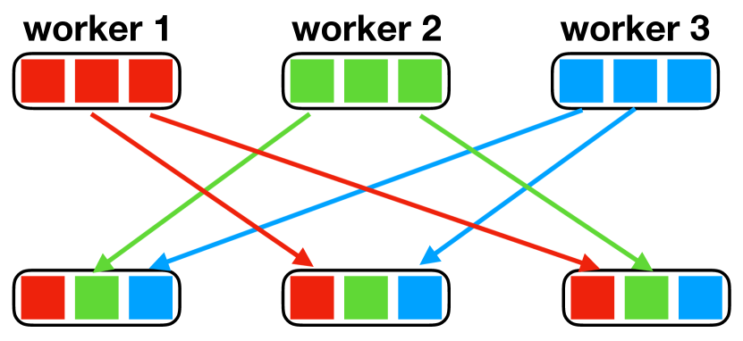
(a) Gather step: Each worker sends its $i$-th chunk to worker $i$.

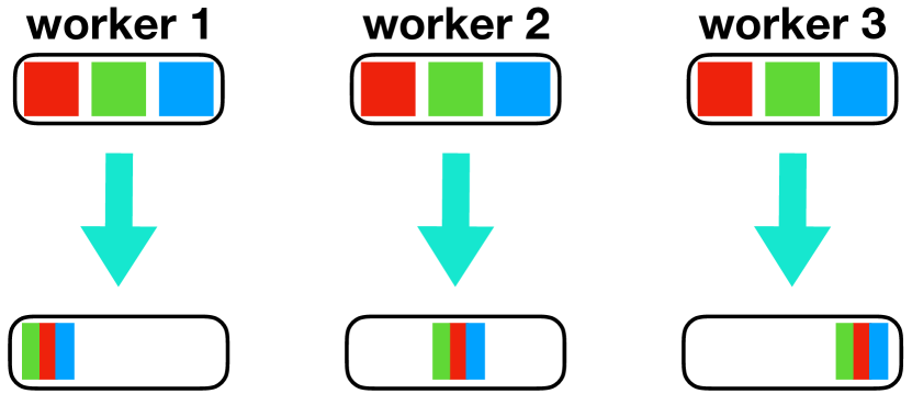
(b) Average step: Each worker averages all chunks it receives.

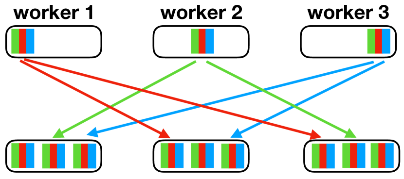
(c) Scatter step: Each worker receives the $i$-th chunk from worker $i$.

Figure 1: Pipeline for Gather-Scatter AllReduce

3.3 APMSqueeze

In APMSqueeze, we only use Adam for a few epochs for warm-up, and after the warm-up stage, we would stop updating $\bm{v}$. The detailed description is stated below.

Consider that there are $n$ workers in the network. In order to fully utilize the bandwidth of the network, we use the Gather-Scatter AllReduce  (Yu et al., 2019a) (See Figure 1) prototype for the realization of the parameter-server parallelism.

Below are the steps of APMSqueeze:

1. Local Computation: Update the error-compensated momentum by $\bm{m}_{t}^{(i)}=\beta_{1}\bm{m}_{t-1}+(1-\beta_{1})\bm{g}_{t}^{(i)}+\bm{\delta}_{t}^{(i)}$, where $\bm{g}_{t}^{(i)}$ is the stochastic gradient, $\beta_{1}$ is the a scalar.

2. Local Compression: Divide $\bm{m}_{t}^{(i)}$ into $n$ chunks, denote the $k$-th chunk of $\bm{m}_{t}^{(i)}$ as $\bm{m}_{t}^{(i,k)}$. Compress each chunk into $\bm{C}_{\omega}\left[\bm{m}_{t}^{(i,k)}\right]$, where $\bm{C}_{\omega}[\cdot]$ is the compression operation, and update the compression error by $\bm{\delta}_{t}^{(i,k)}=\bm{m}_{t}^{(i,k)}-\bm{C}_{\omega}[\bm{m}_{t}^{(i,k)}]$.

3. Scatter: Send the $k$-th chunk $\bm{C}_{\omega}\left[\bm{m}_{t}^{(i,k)}\right]$ to worker $k$, and receive the $i$-th chunk of $\bm{C}_{\omega}\left[\bm{m}_{t}^{(k,i)}\right]$ from worker $k$ for all $k\in\{1,\cdots,n\}$.

4. Local Average: Updating the averaged momentum with $\overline{\bm{m}}_{t}^{(:,i)}=\frac{1}{n}\sum_{k=1}^{n}\bm{C}_{\omega}\left[\bm{m}_{t}^{(k,i)}\right]+\overline{\bm{\delta}}_{t-1}^{(:,i)}$. Recompress $\overline{\bm{m}}_{t}^{(:,i)}$ into $\bm{C}_{\omega}\left[\overline{\bm{m}}_{t}^{(:,i)}\right]$ and update the compression error by $\overline{\bm{\delta}}_{t}^{(:,i)}=\frac{1}{n}\sum_{j=1}^{n}\bm{C}_{\omega}\left[\bm{m}_{t}^{(j,i)}\right]+\overline{\bm{\delta}}_{t-1}^{(:,i)}-\bm{C}_{\omega}\left[\overline{\bm{m}}_{t}^{(:,i)}\right]$.

5. Gather: Send $\bm{C}_{\omega}\left[\overline{\bm{m}}_{t}^{(:,i)}\right]$ to all the workers. After receiving $\bm{C}_{\omega}\left[\overline{\bm{m}}_{t}^{(:,k)}\right]$ from all other workers, replace the $k$-th chunk of the original momentum with $\bm{m}_{t}^{(i,k)}=\bm{C}_{\omega}\left[\overline{\bm{m}}_{t}^{(:,k)}\right]$, which leads to $\bm{m}_{t}=\left(\bm{C}_{\omega}\left[\overline{\bm{m}}_{t}^{(:,1)}\right],\cdots,\bm{C}_{\omega}\left[\overline{\bm{m}}_{t}^{(:,n)}\right]\right)$

6. Model Update: Update the model according to $\bm{x}_{t+1}=\bm{x}_{t}-\gamma_{t}\bm{m}_{t}\oslash\sqrt{\bm{v}_{{}_{\tiny T_{w}}}},$ where $\gamma_{t}$ is the learning rate and $v_{T_{w}}$ is the variance term computed at the end of the warmup step.

Finally, the proposed APMSqueeze algorithm is summarized in Algorithm 1.

4 Theoretical Analysis

In this section, we first introduce some assumptions that is necessary, then we present the theoretical guarantee of the convergence rate for APMSqueeze.

Assumption 1.

We make the following assumptions:

1. Lipschitzian gradient: $f(\cdot)$ is assumed to be with $L$-Lipschitzian gradients, which means

   $$\|\nabla f(\bm{x})-\nabla f(\bm{y})\|\leq L\|\bm{x}-\bm{y}\|,\quad\forall\bm{x},\forall\bm{y},$$

2. Bounded variance: The variance of the stochastic gradient is bounded

   $$\mathbb{E}_{\zeta\sim\mathcal{D}_{i}}\|\nabla F(\bm{x};\bm{\zeta})-\nabla f(\bm{x})\|^{2}\leq\sigma^{2},\quad\forall\bm{x},\forall i.$$

3. Bounded magnitude of error for $C_{\omega}[\cdot]$: The magnitude of worker’s local errors $\bm{\delta}_{t}^{(i,k)}$ and the server’s global error $\overline{\bm{\delta}}_{t}^{(:,i)}$, are assumed to be bounded by a constant $\epsilon$

   $$\sum_{k=1}^{n}\mathbb{E}_{\omega}\left\|\bm{\delta}_{t}^{(i,k)}\right\|\leq\frac{\epsilon}{2},\quad\forall t,\forall i,\quad\sum_{i=1}^{n}\mathbb{E}_{\omega}\left\|\overline{\bm{\delta}}_{t}^{(:,i)}\right\|\leq\frac{\epsilon}{2},\quad\forall t.$$

Next we are ready to present the main theorem for APMSqueeze.

Theorem 1.

Under Assumption 1, for APMSqueeze, we have the following convergence rate

$$\left(1-\frac{\gamma L}{v_{\min}}-\frac{2\gamma^{2}L^{2}}{(1-\beta)^{2}v_{\min}^{2}}\right)\sum_{t=0}^{T}\mathbb{E}\|\nabla f(\bm{x}_{t})\|^{2}_{V}$$

$$\leq \frac{2\mathbb{E}f(\bm{x}_{0})-2\mathbb{E}f(\bm{x}^{*})}{\gamma}+\frac{6\gamma^{2}L^{2}\epsilon^{2}T}{(1-\beta)^{2}v_{\min}^{3}}+\frac{L\gamma\sigma^{2}T}{nv_{\min}}+\frac{2\gamma^{2}L^{2}\sigma^{2}T}{n(1-\beta)^{2}v_{\min}^{2}},$$ (3)

where $V=\text{diag}\left(1/\bm{v}_{T_{w}}^{(1)},1/\bm{v}_{T_{w}}^{(2)},\cdots,1/\bm{v}_{T_{w}}^{(d)}\right)$ is a diagonal matrix spanned by $\bm{v}_{T_{w}}$ and $v_{\min}=\min\{\bm{v}_{T_{w}}^{(1)},\bm{v}_{T_{w}}^{(2)},\cdots,\bm{v}_{T_{w}}^{(d)}\}$ is the mimimum value in $\bm{v}_{T_{w}}$

Given the generic result in Theorem 1, we obtain the convergence rate for APMSqueeze with appropriately chosen the learning rate $\gamma$.

Corollary 1.

Under Assumption 1, for APMSqueeze, choosing $\gamma=\frac{1}{4L(v_{\min})^{-1}+\sigma\sqrt{\frac{T}{n}}+\epsilon^{\frac{2}{3}}T^{\frac{1}{3}}(v_{\min})^{-1}},$ we have the following convergence rate

$$\frac{1}{Tv_{\min}}\sum_{t=0}^{T-1}\mathbb{E}\|\nabla f(\bm{x}_{t})\|^{2}_{V}\lesssim\frac{\sigma}{\sqrt{nT}}+\frac{\epsilon^{\frac{2}{3}}}{T^{\frac{2}{3}}}+\frac{1}{T},$$

where we treat $f(\bm{x}_{1})-f^{*}$, $\beta$ and $L$ as constants.

This result suggests that

• (Comparison to SGD) DoubleSqueeze essentially admits the same convergence rate as SGD in the sense that both of them admit the asymptotical convergence rate $O(1/\sqrt{T})$;

• (Linear Speedup) The asymptotical convergence rate of APMSqueeze is $O(1/\sqrt{nT})$, the same convergence rate as Parallel SGD. It implies that the averaged sample complexity is $O(1/(n\epsilon^{2}))$.

5 Experiments

Table 1: Results on GLUE. BERT-Base (original) and BERT-Large(original) results are from Devlin et al. (2019); BERT-Base (uncompressed) and BERT-Large (uncompressed) are the results that uses the full-precision BertAdam and the same training parameters with the APMSqueeze for training; BERT-Base (compressed) and BERT-Large (compressed) are te results using $\texttt{APMSqueeze}.$ The scores are the median scores over 10 runs. We report the accuracy results for those tasks.

Model	RTE	MRPC	CoLA	SST-2	QNLI	QQP	MNLI-(m/mm)
BERT-Base (original)	66.4	84.8	52.1	93.5	90.5	89.2	84.6/83.4
BERT-Base (uncompressed)	68.2	84.8	56.8	91.8	90.9	90.9	83.6/83.5
BERT-Base (compressed)	69.0	84.8	55.6	91.6	90.8	90.9	83.6/83.9
BERT-Large (original)	70.1	85.4	60.5	94.9	92.7	89.3	86.7/85.9
BERT-Large (uncompressed)	70.3	86.0	60.3	93.1	92.2	91.4	86.1/86.2
BERT-Large (compressed)	70.4	86.1	62.0	93.8	91.9	91.5	85.7/85.4

We validate our theory with experiments that compared APMSqueeze with other implementations. We evaluate the performance of our algorithm for both BERT-Base ,BERT-Large, and ResNet-18. We show that the APMSqueeze converges similar to Adam without compression, but runs much faster than uncompressed algorithms when bandwidth is limited.

5.1 Compression Method

We use the two compression methods described below:

• 1-bit compression: The gradients are quantized into 1-bit representation (containing the sign of each element). Accompanying the vector, a scaling factor is computed as $\frac{\text{magnitude of compensated gradient}}{\text{magnitude of quantized gradient}}.$ The scaling factor is multiplied onto the quantized gradient whenever the quantized gradient is used, so that the recovered gradient has the same magnitude of the compensated gradient. This compression could reduce the $97\%$ communication cost of the original for float32 type training and $94\%$ for float16 type training.

• Top-$k$ compression: We take top $k\%$ elements of the original gradient that is sorted by its absolute magnitude. The communication cost is reduced into $k\%$ of the original.

For BERT-Base and BERT-Large, we use $1$-bit compression. For ResNet-18, we use both $1$-bit compression and Top-$k$ compression.

5.2 BERT Training

Dataset and models

We benchmark the performance of APMSqueeze for both BERT-Base ($L=12$, $H=768$, $A=12$ , $110M$ params) and BERT-Large ($L=24$, $H=1024$, $A=16$, $340M$ params). For pretrain task, the dataset is the same as Devlin et al. (2019), which is a concatenation of Wikipedia and BooksCorpus with $2.5B$ and $800M$ words respectively. For fine-tuning task, we use the GLUE benchmark (Wang et al., 2018).

Hardware

For BERT-Base, we use 32 GPUs resident on 2 servers, and for BERT-Large we use 128 GPUs resident on 8 servers. Each macine has 16 GPUs and each GPU is treated as a single worker. The total batch-size is $4K$ for both tasks.

Training Parameters

For pre-training, the learning rate would linearly increase to $4\times 10^{-4}$ for warm-up in the first $12.5k$ steps, and then decays into $0.99$ of the original after every $520$ steps. We set the two parameters in Algorithm 1 as $\beta_{1}=0.9$ and $\beta_{2}=0.999$. Unlike previous work (Devlin et al., 2019), where they use $90\%$ training step for a sequence length of 128 and then increase the sequence length to 512 for both BERT-Base and BERT-Large. In our experiment, for BERT-Base, $118k$ steps are used for 128 sequence length training and $22k$ steps use a sequence length of 512; while for BERT-Large, $152k$ steps are used for 128 sequence length training and $10k$ steps use a sequence length of 512. When using sequence 128, the Adam pre-conditioned step before compression for BERT-Base is $16k$ and $23k$ for BERT-Large. When using sequence length 512, we use $1.5k$ steps of Adam pre-conditioned steps for both tasks.

Convergence Results

In Figure 3, we report the sample-wise convergence result for the pretrain task using sequence length of 128, which consists most of the training steps. We use the BertAdam (Devlin et al., 2019) optimizer as the uncompressed baseline. From those two figures we shall see that after the Adam pre-conditioned stage, the training effciency remains almost the same for the compressed training and the uncompressed one, while the communication is reduced into $6\%$ of the original.

GLUE Results

For GLUE we consider perform the single-task training on the dev set. In fintuning, we serach over the hyperparameter space with batch sizes $\in\{8,16\}$ and learning rates $\in\{1\times 10^{-5},3\times 10^{-5},5\times 10^{-5},8\times 10^{-5}\}$. Other setting are the same as pre-train task. We report the median development set results for each task over 10 random initializations.

Results are presented in Table 1. We compare our results with the uncompressed training baseline that uses the same training parameters with the compressed one for a fair comparison. We shall see that the compressed training could achieve a comparable performance with the uncompressed baseline. We also include the results from the previous work Devlin et al. (2019).

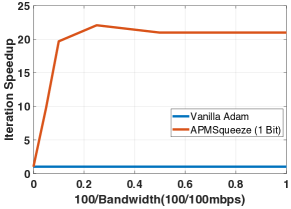
Figure 2: Per-iteration speedup for BERT-base under different network bandwidth

Per-Iteration Speed-up

Figure 2 shows the speed-up performance of our compressed algorithm. We use 64 GPUs and treat each as a separate worker. We train the BERT-Base model from scratch. The communication backend is OpenMPI 4.0.3 compiled with CUDA-aware support. With the proposed algorithm, we compress the communication data from 32bits to 1bit and then report the speed-up of iteration time under different network conditions. Specifically, we use traffic control utility tc to shape the bandwidth from 100Gbits to 100Mbits. With the network going slow, the compressed case can achieve a stable speedup by around 22$\times$ over the uncompressed case. We already reached $10\times$ speed-up for 2Gbits bandwidth and $3\times$ for 10Gbits bandwidth.

End-to-end Speed-up

When consider the end-to-end speed-up we also need to factor in the pre-condition phase, in which we have to run Adam with full precision. In our experiments, we set the pre-condition run as the first 15% of the execution. When the network is 10Gbits we obtain 2$\times$ end-to-end speed-up, while when the network is 1Gbits, we obtain 7$\times$ end-to-end speed-up.

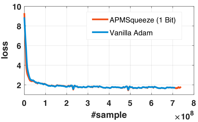
(a) BERT-Base 128

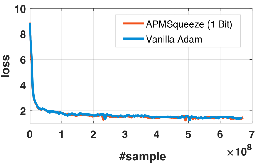
(b) BERT-Large 128

Figure 3: Epoch-wise Convergence Speed (pretrain) for BERT using Sequence Length 128

5.3 ResNet on CIFAR10

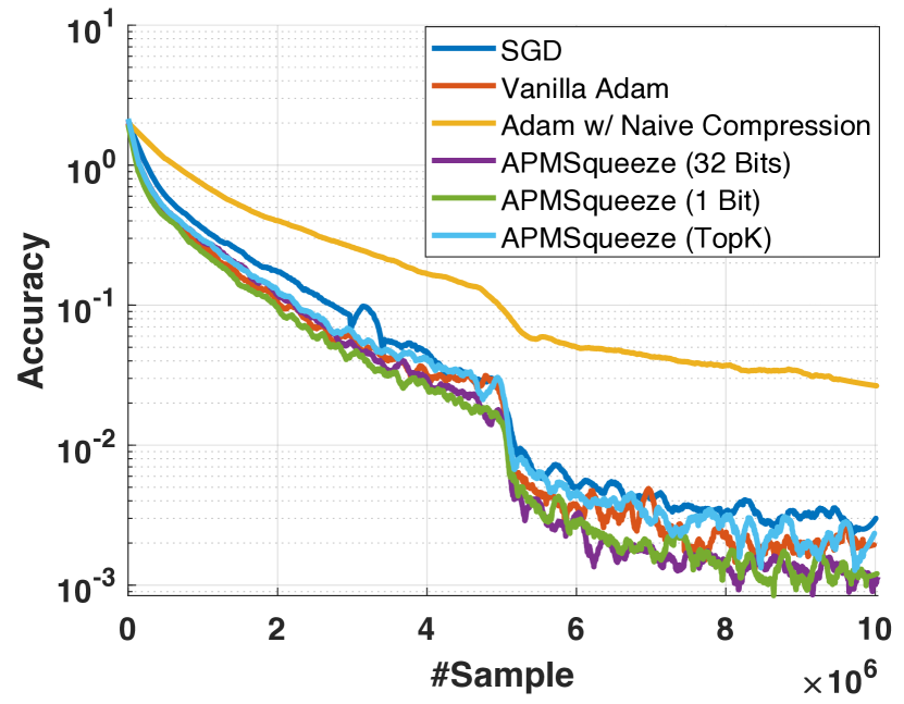
(a) Training Loss

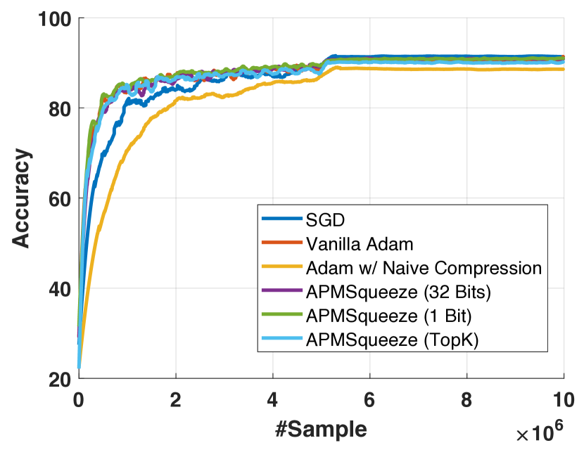
(b) Testing Accuracy

Figure 4: Epoch-wise Convergence Speed for ResNet-18

Dataset

We benchmark the algorithms using a standard image classification task: training CIFAR10 using ResNet-18 (He et al., 2016). This dataset has a training set of 50,000 images and a test set of 10,000 images, where each image is given one of the 10 labels.

Hardware

We run the experiments on $8$ 1080Ti GPUs, each GPU is used as one worker. Here the batch-size on each worker is $128$, therefore the total batch-size is $1024$.

Implementations and setups

We evaluate five implementations for comparison:

1. Original Adam. This is essentially the original Adam (Kingma and Ba, 2014) implementation. We grid search the learning rate $\in\{1\times 10^{-2},1\times 10^{-3},1\times 10^{-4},1\times 10^{-5}\}$, and choose the best learning rate $1e-4$.

2. APMSqueeze (Compressed). This is essentially our APMSqueeze algorithm. We use $13$ epochs for Adam pre-conditioned and the total training takes $200$ epochs. The learning rate $1\times 10^{-4}$ is the same as the original Adam.

3. APMSqueeze (Uncompressed). This is an uncompressed version of the APMSqueeze, which means we do not compress after the Adam pre-conditioned stage but still stops updating $\bm{v}$. We use $13$ epochs for Adam pre-conditioned and the total training takes $200$ epochs. The learning rate $1\times 10^{-4}$ is the same as the original Adam.

4. APGSqueeze. Instead of communicating the momentum $\bm{m}_{t}$, we use the Error-Compensate compression strategy for communicating the gradient $\bm{g}_{t}$. We use $13$ epochs for Adam pre-conditioned and the total training takes $200$ epochs. The learning rate $1\times 10^{-4}$ is the same as the original Adam.

5. SGD. This is vanilla SGD without compression. We grid search the learning rate $\in\{5\times 10^{-1},1\times 10^{-1},1\times 10^{-2},1\times 10^{-3}\}$, and choose the best learning rate $1\times 10^{-1}$.

Notice that the learning rate is decayed into $10\%$ of the original after every $100$ epochs.

Convergence Results

In Figure 4, we report the sample-wise convergence result for each algorithm. We shall see that after the Adam pre-conditioned stage, the training efficiency remains almost the same for the compressed training and the uncompressed one, while the communication is reduced $97\%$ of the original Adam.

Conclusions In this paper, we propose an error compensated Adam preconditioned momentum SGD algorithm (APMSqueeze), which enables a compressed communication but could still achieve almost the same convergence rate with Adam. As a result, the communication overhead can be reduced into $3\%$ of the original and substantially accelerate the training speed under limited network bandwidth. Our theoretical analysis that APMSqueeze admits a linear speed w.r.t the number of workers in the network, and is robust to any compression method. We validate the performance of APMSqueeze empirically for training BERT-base, BERT-large and ResNet-18.

6 Broader Impact

In this paper, we propose a communication efficient algorithm that admits almost the same convergence rate with Adam, but achieves 10-30$\times$ speedup corresponding to the communication overhead.

Adam, which uses a more complicated updating rule than SGD, has shown to be a very efficient optimizer due to its fast convergence speed, and is even necessary for some large-scale machine learning tasks, such as BERT. With the increasing number of parameters in model machine learning models, it has become necessary to use large-scale (hundreds or even thousands of workers) parallel training, and the communication overhead could be comparable or even substantially overweight the computation cost for this large-scale training task. Therefore it is very important to design a communication efficient algorithm for Adam. However, there was no communication efficient algorithm proposed before due to the intrinsic non-linearity of Adam. To our knowledge, we are the first work that solve this problem. We want to emphasize that our method (using Adam as preconditioned warmup) could not only reduce a great amount ($97\%$) of communication cost, but also can be transferred to other applications of Adam, such as decentralized training, which is also a widely used method for reducing the communication overhead when the network latency is high.

Supplementary

7 Proof to the Updating Form

Since our algorithm is equivalent to running a parameter-server prototype communication on each chunk of the gradient, so below we will assume a parameter-server model (which means the tensor is not required to be divided into $n$ chunks) for simplicity.

According to the algorithm description in Section 3.3, at iteration $t+1$, the updating step of the momentum term $\bm{m}_{t+1}$ can be divided into two steps:

1. Local Update and Compress: each worker locally update $\bm{m}_{t}$ and use the error-compensate strategy for compressing.

   $$\bm{m}_{t}^{(i)}= \beta\bm{m}_{t}+(1-\beta)\bm{g}_{t}^{(i)}$$

   $$\bm{m}_{t+\frac{1}{2}}^{(i)}= C_{\omega}[\bm{m}_{t}^{(i)}+\bm{\delta}_{t}^{(i)}]$$

   $$\bm{\delta}_{t+1}^{(i)}= \bm{m}_{t}^{(i)}+\bm{\delta}_{t}^{(i)}-\bm{m}_{t+\frac{1}{2}}^{(i)}.$$

2. All workers send its $\bm{m}_{t+\frac{1}{2}}^{(i)}$ to the server. The server takes the average over them and compress it again using error-compensation.

   $$\bm{m}_{t+\frac{1}{2}}= \frac{1}{n}\sum_{i=1}^{n}\bm{m}_{t+\frac{1}{2}}^{(i)}$$

   $$\bm{m}_{t+1}= C_{\omega}[\bm{m}_{t+\frac{1}{2}}+\bm{\delta}_{t}]$$

   $$\bm{\delta}_{t+1}= \bm{m}_{t+\frac{1}{2}}+\bm{\delta}_{t}-\bm{m}_{t+1}.$$

3. The server broadcast $\bm{m}_{t+1}$ to all workers, and all workers update the local model according to

   $$\bm{x}_{t+1}=\bm{x}_{t}-\bm{\gamma}\bm{m}_{t+1}\oslash\sqrt{\bm{v}_{T_{w}}^{2}}.$$

So actually the updating rule above can be summarized as

$$\bm{m}_{t+1}= C_{\omega}[\bm{m}_{t+\frac{1}{2}}+\bm{\delta}_{t}]$$

$$= \bm{m}_{t+\frac{1}{2}}+\bm{\delta}_{t}-\bm{\delta}_{t+1}\quad\text{(from the definition of $\bm{\delta}_{t+1}$)}$$

$$= \frac{1}{n}\sum_{i=1}^{n}C_{\omega}[\bm{m}_{t}^{(i)}+\bm{\delta}_{t}^{(i)}]+\bm{\delta}_{t}-\bm{\delta}_{t+1}$$

$$= \frac{1}{n}\sum_{i=1}^{n}\left(\bm{m}_{t}^{(i)}+\bm{\delta}_{t}^{(i)}-\bm{\delta}_{t+1}^{(i)}\right)+\bm{\delta}_{t}-\bm{\delta}_{t+1}\quad\text{(from the definition of $\bm{\delta}_{t+1}^{(i)}$)}$$

$$= \beta\bm{m}_{t}+\frac{1-\beta}{n}\sum_{i=1}^{n}\bm{g}_{t}^{(i)}+\left(\frac{1}{n}\sum_{i=1}^{n}\bm{\delta}_{t}^{(i)}+\bm{\delta}_{t}\right)-\left(\frac{1}{n}\sum_{i=1}^{n}\bm{\delta}_{t+1}^{(i)}+\bm{\delta}_{t+1}\right).$$

Denote

$$\overline{\bm{g}}_{t}= \frac{1}{n}\sum_{i=1}^{n}\bm{g}_{t}^{(i)}$$

$$\overline{\bm{\delta}}_{t}= \frac{1}{n}\sum_{i=1}^{n}\bm{\delta}_{t}^{(i)}+\bm{\delta}_{t},$$

the update rule of $\bm{m}_{t}$ can be summarized as

$$\bm{m}_{t}=\beta\bm{m}_{t-1}+(1-\beta)\overline{\bm{g}}_{t}+\overline{\bm{\delta}}_{t-1}-\overline{\bm{\delta}}_{t},$$

and

$$\bm{x}_{t+1}=\bm{x}_{t}-\gamma V\bm{m}_{t},$$

where $V=\text{diag}(1/\sqrt{v_{1}},1/\sqrt{v_{2}},\cdots,1/\sqrt{v_{d}})$ is the a diagonal matrix that spanned with $\bm{v}_{T_{w}}$.

8 Proof to Theorem 1

Notice that in for APMSqueeze, the learning rate for each coordinate is different. In order to simplify our analysis, we instead consider another function that is defined as

$$H(\bm{z})=F(V^{\frac{1}{2}}\bm{z}),$$

also

$$h(\bm{z})=f(V^{\frac{1}{2}}\bm{z}),$$

where ${V}$ is a diagonal matrix.

In this case we have

$${V}^{\frac{1}{2}}\nabla f({V}^{\frac{1}{2}}\bm{z})=\nabla h(\bm{z}).$$

Therefore the updating rule of APMSqueeze in the view of $h(\cdot)$ is

$${V}^{\frac{1}{2}}\bm{z}_{t+1}={V}^{\frac{1}{2}}\bm{z}_{t}-\gamma{V}^{\frac{1}{2}}\left({V}^{\frac{1}{2}}\bm{m}_{t}\right).$$

It can be easily verified that

$$\bm{m}_{t}= (1-\beta)\sum_{s=0}^{t}\beta^{t-s}\overline{\bm{g}}_{s}+\sum_{s=0}^{t}\beta^{t-s}(\overline{\bm{\delta}}_{s-1}-\overline{\bm{\delta}}_{s})$$

$$= (1-\beta)\sum_{s=0}^{t}\beta^{t-s}\frac{1}{n}\sum_{i=1}^{n}\nabla F(V^{\frac{1}{2}}\bm{z}_{t};\xi_{t}^{(i)})+\sum_{s=0}^{t}\beta^{t-s}(\overline{\bm{\delta}}_{s-1}-\overline{\bm{\delta}}_{s})$$

which means

$${V}^{\frac{1}{2}}\bm{m}_{t}= (1-\beta)\sum_{s=0}^{t}\beta^{t-s}\frac{1}{n}\sum_{i=1}^{n}{V}^{\frac{1}{2}}\nabla F(V^{\frac{1}{2}}\bm{z}_{t};\xi_{t}^{(i)})+\sum_{s=0}^{t}\beta^{t-s}{V}^{\frac{1}{2}}(\overline{\bm{\delta}}_{s-1}-\overline{\bm{\delta}}_{s})$$

$$= (1-\beta)\sum_{s=0}^{t}\beta^{t-s}\frac{1}{n}\sum_{i=1}^{n}\nabla H(V^{\frac{1}{2}}\bm{z}_{t};\xi_{t}^{(i)})+\sum_{s=0}^{t}\beta^{t-s}{V}^{\frac{1}{2}}(\overline{\bm{\delta}}_{s-1}-\overline{\bm{\delta}}_{s})$$

$$= (1-\beta)\sum_{s=0}^{t}\beta^{t-s}\overline{\bm{g}}_{s}(\bm{z})+\sum_{s=0}^{t}\beta^{t-s}{V}^{\frac{1}{2}}(\overline{\bm{\delta}}_{s-1}-\overline{\bm{\delta}}_{s}),$$

where $\overline{\bm{g}}_{s}(\bm{z})$ is the corresponding averaged stochastic gradient computed in the view of loss function $h(\cdot)$.

Then, if we define $\bm{m}_{t}(\bm{z})={V}^{\frac{1}{2}}\bm{m}_{t}$, the updating rule of $\bm{m}_{t}(z)$ admits

$$\bm{m}_{t}(\bm{z})=\beta\bm{m}_{t-1}(\bm{z})+(1-\beta)\overline{\bm{g}}_{t}(\bm{z})+{V}^{\frac{1}{2}}\overline{\bm{\delta}}_{t-1}-{V}^{\frac{1}{2}}\overline{\bm{\delta}}_{t},$$ (4)

and

$${V}^{\frac{1}{2}}\bm{z}_{t+1}= {V}^{\frac{1}{2}}\bm{z}_{t}-\gamma{V}^{\frac{1}{2}}\bm{m}_{t}(\bm{z})$$

$$\bm{z}_{t+1}= \bm{z}_{t}-\gamma\bm{m}_{t}(\bm{z}).$$ (5)

From (4) and (5) we shall see that using different learning rate for each coordinate is equivalent to optimizing a new loss function defined on scaling the original coordinate and using a uniform learning for all coordinates. Therefore below we first study the behavior of the error-compensated momentum SGD using a constant learning rate.

Below are some critical lemmas for the proof of Theorem 1.

Lemma 1.

Given two non-negative sequences $\{a_{t}\}_{t=1}^{\infty}$ and $\{b_{t}\}_{t=1}^{\infty}$ that satisfying

$$a_{t}=\sum_{s=1}^{t}\rho^{t-s}b_{s},$$ (6)

with $\rho\in[0,1)$, we have

$$D_{k}:=\sum_{t=1}^{k}a_{t}^{2}\leq \frac{1}{(1-\rho)^{2}}\sum_{s=1}^{k}b_{s}^{2}.$$

Proof.

From the definition, we have

$$S_{k}= \sum_{t=1}^{k}\sum_{s=1}^{t}\rho^{t-s}b_{s}=\sum_{s=1}^{k}\sum_{t=s}^{k}\rho^{t-s}b_{s}=\sum_{s=1}^{k}\sum_{t=0}^{k-s}\rho^{t}b_{s}\leq\sum_{s=1}^{k}{b_{s}\over 1-\rho},$$ (7)

$$D_{k}= \sum_{t=1}^{k}\sum_{s=1}^{t}\rho^{t-s}b_{s}\sum_{r=1}^{t}\rho^{t-r}b_{r}$$

$$= \sum_{t=1}^{k}\sum_{s=1}^{t}\sum_{r=1}^{t}\rho^{2t-s-r}b_{s}b_{r}$$

$$\leq \sum_{t=1}^{k}\sum_{s=1}^{t}\sum_{r=1}^{t}\rho^{2t-s-r}{b_{s}^{2}+b_{r}^{2}\over 2}$$

$$= \sum_{t=1}^{k}\sum_{s=1}^{t}\sum_{r=1}^{t}\rho^{2t-s-r}b_{s}^{2}$$

$$\leq {1\over 1-\rho}\sum_{t=1}^{k}\sum_{s=1}^{t}\rho^{t-s}b_{s}^{2}$$

$$\leq {1\over(1-\rho)^{2}}\sum_{s=1}^{k}b_{s}^{2},\quad\text{(due to \eqref{eqn3})}$$

which completes the proof. ∎

Lemma 2.

Under Assumption 1, for any sequence that follows the updating rule of

$$\bm{x}_{t+1}= \bm{x}_{t}-\gamma\bm{m}_{t}$$

$$\bm{m}_{t}= \beta\bm{m}_{t-1}+(1-\beta)\overline{\bm{g}}_{t}+\overline{\bm{\delta}}_{t-1}-\overline{\bm{\delta}}_{t},$$

if

$$\mathbb{E}\overline{\bm{g}}_{t}=\nabla f(\bm{x}_{t}),\quad\mathbb{E}\|\overline{\bm{g}}_{t}-\nabla f(\bm{x}_{t})\|^{2}\leq\frac{\sigma^{2}}{n},\quad\mathbb{E}\|\overline{\bm{\delta}}_{t}\|^{2}\leq\epsilon^{2},\quad\forall t,$$

$$\|\nabla f(\bm{x})-\nabla f(\bm{y})\|\leq L\|\bm{x}-\bm{y}\|,\quad\forall\bm{x},\forall\bm{y},$$

then we can guarantee that

$$\left(1-\gamma L-\frac{2\gamma^{2}L^{2}}{(1-\beta)^{2}}\right)\sum_{t=0}^{T}\mathbb{E}\|\nabla f(\bm{x}_{t})\|^{2}$$

$$\leq \frac{2\mathbb{E}f(\bm{x}_{1})-2\mathbb{E}f(\bm{x}^{*})}{\gamma}+\frac{6\gamma^{2}L^{2}\epsilon^{2}T}{(1-\beta)^{2}}+\frac{L\gamma\sigma^{2}T}{n}+\frac{2\gamma^{2}L^{2}\sigma^{2}T}{n(1-\beta)^{2}}$$

Proof.

Instead of investigating $\bm{x}_{t}$ directly, we introduce the following sequence

$$\bm{y}_{t}=\bm{x}_{t}-\frac{\gamma}{1-\beta}(\bm{m}_{t}+\overline{\bm{\delta}}_{t-1}).$$

The updating rule of $\bm{y}_{t}$ admits

$$\bm{y}_{t+1}-\bm{y}_{t}= \bm{x}_{t+1}-\bm{x}_{t}-\frac{\gamma}{1-\beta}(\bm{m}_{t+1}-\bm{m}_{t}-\overline{\bm{\delta}}_{t+1}+\overline{\bm{\delta}}_{t})$$

$$= -\gamma\bm{m}_{t}-\frac{\gamma}{1-\beta}(\beta\bm{m_{t}}+(1-\beta)\bm{g}_{t}+\overline{\bm{\delta}}_{t-1}-\overline{\bm{\delta}}_{t}-\bm{m}_{t}+\overline{\bm{\delta}}_{t}-\overline{\bm{\delta}}_{t-1})$$

$$= -\gamma\bm{g}_{t}.$$

Since $f(\cdot)$ is with L-Lipschitzian, we have

$$\mathbb{E}f(\bm{y}_{t+1})-\mathbb{E}f(\bm{y}_{t})\leq \mathbb{E}\left\langle\nabla f(\bm{y}_{t}),\bm{y}_{t+1}-\bm{y}_{t}\right\rangle+\frac{L}{2}\mathbb{E}\left\|\bm{y}_{t+1}-\bm{y}_{t}\right\|^{2}$$

$$= -\gamma\mathbb{E}\left\langle\nabla f(\bm{y}_{t}),\bm{g}_{t}\right\rangle+\frac{L\gamma^{2}}{2}\mathbb{E}\|\bm{g}_{t}\|^{2}$$

$$= -\gamma\mathbb{E}\left\langle\nabla f(\bm{y}_{t}),\nabla f(\bm{x}_{t})\right\rangle+\frac{L\gamma^{2}}{2}\mathbb{E}\|\bm{g}_{t}\|^{2}$$

$$= -\frac{\gamma}{2}\mathbb{E}\|\nabla f(\bm{x}_{t})\|^{2}-\frac{\gamma}{2}\mathbb{E}\|\nabla f(\bm{y}_{t})\|^{2}+\frac{\gamma}{2}\mathbb{E}\|\nabla f(\bm{x}_{t})-\nabla f(\bm{y}_{t})\|^{2}+\frac{L\gamma^{2}}{2}\mathbb{E}\|\bm{g}_{t}\|^{2}$$

$$\leq -\frac{\gamma}{2}\mathbb{E}\|\nabla f(\bm{x}_{t})\|^{2}+\frac{\gamma L^{2}}{2}\mathbb{E}\|\bm{x}_{t}-\bm{y}_{t}\|^{2}+\frac{L\gamma^{2}}{2}\mathbb{E}\|\bm{g}_{t}\|^{2}$$

$$= -\frac{\gamma}{2}\mathbb{E}\|\nabla f(\bm{x}_{t})\|^{2}+\frac{\gamma^{3}L^{2}}{2}\mathbb{E}\left\|\frac{\bm{m}_{t}}{1-\beta}+\frac{\overline{\bm{\delta}}_{t-1}}{1-\beta}\right\|^{2}+\frac{L\gamma^{2}}{2}\mathbb{E}\|\bm{g}_{t}\|^{2}$$

$$\leq -\frac{\gamma}{2}\mathbb{E}\|\nabla f(\bm{x}_{t})\|^{2}+\frac{\gamma^{3}L^{2}}{(1-\beta)^{2}}\mathbb{E}\|\bm{m}_{t}\|^{2}+\frac{\gamma^{3}L^{2}}{(1-\beta)^{2}}\mathbb{E}\|\overline{\bm{\delta}}_{t-1}\|^{2}+\frac{L\gamma^{2}}{2}\mathbb{E}\|\bm{g}_{t}\|^{2}$$

$$\leq -\frac{\gamma}{2}\mathbb{E}\|\nabla f(\bm{x}_{t})\|^{2}+\frac{\gamma^{3}L^{2}}{(1-\beta)^{2}}\mathbb{E}\|\bm{m}_{t}\|^{2}+\frac{\gamma^{3}L^{2}\epsilon^{2}}{(1-\beta)^{2}}+\frac{L\gamma^{2}}{2}\mathbb{E}\|\bm{g}_{t}\|^{2}$$

$$\leq -\frac{\gamma}{2}\mathbb{E}\|\nabla f(\bm{x}_{t})\|^{2}+\frac{\gamma^{3}L^{2}}{(1-\beta)^{2}}\mathbb{E}\|\bm{m}_{t}\|^{2}+\frac{\gamma^{3}L^{2}\epsilon^{2}}{(1-\beta)^{2}}+\frac{L\gamma^{2}}{2}\mathbb{E}\|\nabla f(\bm{x}_{t})\|^{2}+\frac{L\gamma^{2}\sigma^{2}}{2n}.$$

Summing up the equation above from $t=0$ to $t=T$ we get

$$\mathbb{E}f(\bm{y}_{T+1})-\mathbb{E}f(\bm{y}_{0})\leq-\frac{(1-\gamma L)\gamma}{2}\sum_{t=0}^{T}\mathbb{E}\|\nabla f(\bm{x}_{t})\|^{2}+\frac{\gamma^{3}L^{2}}{(1-\beta)^{2}}\sum_{t=0}^{T}\mathbb{E}\|\bm{m}_{t}\|^{2}+\frac{\gamma^{3}L^{2}\epsilon^{2}T}{(1-\beta)^{2}}+\frac{L\gamma^{2}\sigma^{2}T}{2n},$$

which can be rewritten into

$$(1-\gamma L)\sum_{t=0}^{T}\mathbb{E}\|\nabla f(\bm{x}_{t})\|^{2}\leq \frac{2\mathbb{E}f(\bm{y}_{0})-2\mathbb{E}f(\bm{y}_{T+1})}{\gamma}+\frac{2\gamma^{2}L^{2}}{(1-\beta)^{2}}\sum_{t=0}^{T}\mathbb{E}\|\bm{m}_{t}\|^{2}+\frac{2\gamma^{2}L^{2}\epsilon^{2}T}{(1-\beta)^{2}}+\frac{L\gamma\sigma^{2}T}{n}.$$ (8)

Notice that we have

$$\bm{m}_{t}= (1-\beta)\sum_{s=0}^{t}\beta^{t-s}\overline{\bm{g}}_{s}+\sum_{s=0}^{t}\beta^{t-s}(\overline{\bm{\delta}}_{s-1}-\overline{\bm{\delta}}_{s})$$

which by using Lemma 1, we have

$$\sum_{t=0}^{T}\|\bm{m}_{t}\|^{2}\leq\sum_{t=0}^{T}\|\bm{g}_{t}\|^{2}+\frac{2}{(1-\beta)^{2}}\sum_{t=0}^{T}\|\overline{\bm{\delta}}_{t}\|^{2}\leq\sum_{t=0}^{T}\|\nabla f(\bm{x}_{t})\|^{2}+\frac{\sigma^{2}T}{n}+\frac{2\epsilon^{2}T}{(1-\beta)^{2}}.$$ (9)

Combing (8) and (9) together we get

$$\left(1-\gamma L-\frac{2\gamma^{2}L^{2}}{(1-\beta)^{2}}\right)\sum_{t=0}^{T}\mathbb{E}\|\nabla f(\bm{x}_{t})\|^{2}$$

$$\leq \frac{2\mathbb{E}f(\bm{y}_{0})-2\mathbb{E}f(\bm{y}_{T+1})}{\gamma}+\frac{6\gamma^{2}L^{2}\epsilon^{2}T}{(1-\beta)^{2}}+\frac{L\gamma\sigma^{2}T}{n}+\frac{2\gamma^{2}L^{2}\sigma^{2}T}{n(1-\beta)^{2}}$$

$$\leq \frac{2\mathbb{E}f(\bm{x}_{1})-2\mathbb{E}f(\bm{x}^{*})}{\gamma}+\frac{6\gamma^{2}L^{2}\epsilon^{2}T}{(1-\beta)^{2}}+\frac{L\gamma\sigma^{2}T}{n}+\frac{2\gamma^{2}L^{2}\sigma^{2}T}{n(1-\beta)^{2}}.$$

∎

Proof to Theorem 1

Since using a per-coordinate learning rate for loss function $f(\cdot)$ is equivalent to use a constant learning for all coordinates but for loss function $h(\cdot)$, the only two thing that change are

• Different L-Lipschitzian coefficient: the L-Lipschitzian coefficient for $h(\cdot)$ is

  $$\|\nabla h(\bm{x})-\nabla h(\bm{y})\|^{2}= \left\|V^{\frac{1}{2}}\nabla f(V^{\frac{1}{2}}\bm{x})-V^{\frac{1}{2}}\nabla f(V^{\frac{1}{2}}\bm{y})\right\|^{2}$$

  $$= \left\|\nabla f(V^{\frac{1}{2}}\bm{x})-\nabla f(V^{\frac{1}{2}}\bm{y})\right\|^{2}_{V}$$

  $$\leq L^{2}\left\|V^{\frac{1}{2}}\bm{x}-V^{\frac{1}{2}}\bm{y}\right\|^{2}_{V}$$

  $$= L^{2}\|\bm{x}-\bm{y}\|^{2}_{V^{2}}$$

  $$\leq L^{2}V_{\max}^{2}\|\bm{x}-\bm{y}\|^{2}.$$

  Therefore the effective L-Lipschitzian coefficient of $h(\bm{x})$ is $LV_{\max}$

• Different definition of $\overline{\bm{\delta}}_{t}$: from (4) we shall see that actually the compression error in the view of $h(\cdot)$ is $V^{\frac{1}{2}}\overline{\bm{\delta}}_{t}$, so in this case we have

  $$\mathbb{E}\|V^{\frac{1}{2}}\overline{\bm{\delta}}_{t}\|^{2}\leq V_{\max}\epsilon^{2}$$

Proof.

From Lemma 2, we have

$$\left(1-\gamma L-\frac{2\gamma^{2}L^{2}V_{\max}^{2}}{(1-\beta)^{2}}\right)\sum_{t=0}^{T}\mathbb{E}\|\nabla h(\bm{z}_{t})\|^{2}$$

$$\leq \frac{2\mathbb{E}f(\bm{x}_{0})-2\mathbb{E}f(\bm{x}^{*})}{\gamma}+\frac{6\gamma^{2}L^{2}\epsilon^{2}V_{\max}^{3}T}{(1-\beta)^{2}}+\frac{L\gamma V_{\max}\sigma^{2}T}{n}+\frac{2\gamma^{2}L^{2}\sigma^{2}V_{\max}^{2}T}{n(1-\beta)^{2}},$$

which by using $\nabla h(\bm{z}_{t})=V^{\frac{1}{2}}\nabla f(\bm{x}_{t})$, it becomes

$$\left(1-\gamma LV_{\max}-\frac{2\gamma^{2}L^{2}V_{\max}^{2}}{(1-\beta)^{2}}\right)\sum_{t=0}^{T}\mathbb{E}\|\nabla f(\bm{x}_{t})\|^{2}_{V}$$

$$\leq \frac{2\mathbb{E}f(\bm{x}_{0})-2\mathbb{E}f(\bm{x}^{*})}{\gamma}+\frac{6\gamma^{2}L^{2}\epsilon^{2}V_{\max}^{3}T}{(1-\beta)^{2}}+\frac{L\gamma V_{\max}\sigma^{2}T}{n}+\frac{2\gamma^{2}L^{2}\sigma^{2}V_{\max}^{2}T}{n(1-\beta)^{2}},$$

Since $V_{\max}=\frac{1}{\sqrt{v_{\min}}}$, therefore the equation above becomes

$$\left(1-\frac{\gamma L}{v_{\min}}-\frac{2\gamma^{2}L^{2}}{(1-\beta)^{2}v_{\min}^{2}}\right)\sum_{t=0}^{T}\mathbb{E}\|\nabla f(\bm{x}_{t})\|^{2}_{V}$$

$$\leq \frac{2\mathbb{E}f(\bm{x}_{0})-2\mathbb{E}f(\bm{x}^{*})}{\gamma}+\frac{6\gamma^{2}L^{2}\epsilon^{2}T}{(1-\beta)^{2}v_{\min}^{3}}+\frac{L\gamma\sigma^{2}T}{nv_{\min}}+\frac{2\gamma^{2}L^{2}\sigma^{2}T}{n(1-\beta)^{2}v_{\min}^{2}},$$

∎

9 Proof to Corollary 1

Proof.

By choosing $\gamma=\frac{1-\beta}{4LV_{\max}+\sigma\sqrt{\frac{T}{n}}+T^{{}^{\frac{1}{3}}}\epsilon^{{}^{\frac{2}{3}}}}$, we can guarantee that

$$1-\gamma L-\frac{2\gamma^{2}L^{2}V_{\max}^{2}}{(1-\beta)^{2}}\geq \frac{1}{2}.$$

So (3) leads to

$$\sum_{t=0}^{T}\mathbb{E}\|\nabla f(\bm{x}_{t})\|^{2}_{V}\leq \frac{2\left(\mathbb{E}f(\bm{y}_{0})-f(\bm{y}^{*})\right)}{(1-\beta)}\left(4LV_{\max}+\sigma\sqrt{\frac{T}{n}}+T^{{}^{\frac{1}{3}}}\epsilon^{{}^{\frac{2}{3}}}\right)$$

$$+\left((1-\beta)L\sqrt{T}+2L^{2}V_{\max}^{2}\right)\frac{\sigma}{\sqrt{n}}+6L^{2}\epsilon^{\frac{2}{3}}T^{\frac{1}{3}}V_{\max}^{3}$$

$$\frac{1}{T}\sum_{t=0}^{T}\mathbb{E}\|\nabla f(\bm{x}_{t})\|^{2}_{V}\leq \frac{2\left(\mathbb{E}f(\bm{y}_{0})-f(\bm{y}^{*})\right)}{(1-\beta)}\left(\frac{4LV_{\max}}{T}+\frac{\sigma}{\sqrt{nT}}+T^{{}^{-\frac{2}{3}}}\epsilon^{{}^{\frac{2}{3}}}\right)$$

$$+\left((1-\beta)L+\frac{2L^{2}V_{\max}^{2}}{\sqrt{T}}\right)\frac{\sigma}{\sqrt{nT}}+6L^{2}\epsilon^{\frac{2}{3}}T^{-\frac{2}{3}}V_{\max}^{3}.$$

Treating $f(\bm{y}_{1})-f^{*}$, $\beta$ and $L$ as constants, from the inequality above we get

$$\frac{1}{T}\sum_{t=0}^{T}\mathbb{E}\|\nabla f(\bm{x}_{t})\|^{2}\lesssim\frac{\sigma}{\sqrt{nT}}+\frac{\epsilon^{\frac{2}{3}}}{T^{\frac{2}{3}}}+\frac{1}{T}.$$

It completes the proof. ∎

References

Agarwal et al. [2018]
N. Agarwal, A. T. Suresh, F. X. X. Yu, S. Kumar, and B. McMahan.
cpSGD: Communication-efficient and differentially-private
distributed SGD.
In S. Bengio, H. Wallach, H. Larochelle, K. Grauman, N. Cesa-Bianchi,
and R. Garnett, editors, Advances in Neural Information Processing
Systems 31, pages 7564–7575. Curran Associates, Inc., 2018.
Alistarh et al. [2017]
D. Alistarh, D. Grubic, J. Li, R. Tomioka, and M. Vojnovic.
QSGD: Communication-Efficient SGD via gradient quantization and
encoding.
In I. Guyon, U. V. Luxburg, S. Bengio, H. Wallach, R. Fergus,
S. Vishwanathan, and R. Garnett, editors, Advances in Neural
Information Processing Systems 30, pages 1709–1720. Curran Associates,
Inc., 2017.
Basu et al. [2019]
D. Basu, D. Data, C. Karakus, and S. Diggavi.
Qsparse-local-sgd: Distributed sgd with quantization, sparsification
and local computations.
In H. Wallach, H. Larochelle, A. Beygelzimer, F. d Alché-Buc,
E. Fox, and R. Garnett, editors, Advances in Neural Information
Processing Systems 32, pages 14695–14706. Curran Associates, Inc., 2019.
Bernstein et al. [2018]
J. Bernstein, J. Zhao, K. Azizzadenesheli, and A. Anandkumar.
signsgd with majority vote is communication efficient and byzantine
fault tolerant.
10 2018.
Chaturapruek et al. [2015]
S. Chaturapruek, J. C. Duchi, and C. Ré.
Asynchronous stochastic convex optimization: the noise is in the
noise and sgd don t care.
In C. Cortes, N. D. Lawrence, D. D. Lee, M. Sugiyama, and R. Garnett,
editors, Advances in Neural Information Processing Systems 28, pages
1531–1539. Curran Associates, Inc., 2015.
Devlin et al. [2019]
J. Devlin, M.-W. Chang, K. Lee, and K. Toutanova.
Bert: Pre-training of deep bidirectional transformers for language
understanding.
In NAACL-HLT, 2019.
Duchi et al. [2011]
J. Duchi, E. Hazan, and Y. Singer.
Adaptive subgradient methods for online learning and stochastic
optimization.
Journal of Machine Learning Research, 12(61):2121–2159, 2011.
URL http://jmlr.org/papers/v12/duchi11a.html.
He et al. [2016]
K. He, X. Zhang, S. Ren, and J. Sun.
Deep residual learning for image recognition.
In 2016 IEEE Conference on Computer Vision and Pattern
Recognition (CVPR), pages 770–778, 2016.
Ivkin et al. [2019]
N. Ivkin, D. Rothchild, E. Ullah, V. braverman, I. Stoica, and R. Arora.
Communication-efficient distributed sgd with sketching.
In H. Wallach, H. Larochelle, A. Beygelzimer, F. d Alché-Buc,
E. Fox, and R. Garnett, editors, Advances in Neural Information
Processing Systems 32, pages 13144–13154. Curran Associates, Inc., 2019.
Jiang and Agrawal [2018]
P. Jiang and G. Agrawal.
A linear speedup analysis of distributed deep learning with sparse
and quantized communication.
In S. Bengio, H. Wallach, H. Larochelle, K. Grauman, N. Cesa-Bianchi,
and R. Garnett, editors, Advances in Neural Information Processing
Systems 31, pages 2530–2541. Curran Associates, Inc., 2018.
Kingma and Ba [2014]
D. Kingma and J. Ba.
Adam: A method for stochastic optimization.
International Conference on Learning Representations, 12 2014.
Kingma and Ba [2015]
D. P. Kingma and J. Ba.
Adam: A method for stochastic optimization.
CoRR, abs/1412.6980, 2015.
Koloskova* et al. [2020]
A. Koloskova*, T. Lin*, S. U. Stich, and M. Jaggi.
Decentralized deep learning with arbitrary communication compression.
In International Conference on Learning Representations, 2020.
URL https://openreview.net/forum?id=SkgGCkrKvH.
Li et al. [2018]
Y. Li, M. Yu, S. Li, S. Avestimehr, N. S. Kim, and A. Schwing.
Pipe-sgd: A decentralized pipelined sgd framework for distributed
deep net training.
In S. Bengio, H. Wallach, H. Larochelle, K. Grauman, N. Cesa-Bianchi,
and R. Garnett, editors, Advances in Neural Information Processing
Systems 31, pages 8056–8067. Curran Associates, Inc., 2018.
Lian et al. [2017]
X. Lian, C. Zhang, H. Zhang, C.-J. Hsieh, W. Zhang, and J. Liu.
Can decentralized algorithms outperform centralized algorithms? a
case study for decentralized parallel stochastic gradient descent.
In I. Guyon, U. V. Luxburg, S. Bengio, H. Wallach, R. Fergus,
S. Vishwanathan, and R. Garnett, editors, Advances in Neural
Information Processing Systems 30, pages 5330–5340. Curran Associates,
Inc., 2017.
Luo et al. [2019]
L. Luo, Y. Xiong, and Y. Liu.
Adaptive gradient methods with dynamic bound of learning rate.
In International Conference on Learning Representations, 2019.
URL https://openreview.net/forum?id=Bkg3g2R9FX.
Phuong and Phong [2020]
T. T. Phuong and L. T. Phong.
Distributed sgd with flexible gradient compression.
IEEE Access, 8:64707–64717, 2020.
Seide et al. [2014]
F. Seide, H. Fu, J. Droppo, G. Li, and D. Yu.
1-bit stochastic gradient descent and application to data-parallel
distributed training of speech dnns.
In Interspeech 2014, September 2014.
Shen et al. [2018]
Z. Shen, A. Mokhtari, T. Zhou, P. Zhao, and H. Qian.
Towards more efficient stochastic decentralized learning: Faster
convergence and sparse communication.
In J. Dy and A. Krause, editors, Proceedings of the 35th
International Conference on Machine Learning, volume 80 of Proceedings
of Machine Learning Research, pages 4624–4633, Stockholmsmässan,
Stockholm Sweden, 10–15 Jul 2018. PMLR.
Shi et al. [2019]
S. Shi, Q. Wang, K. Zhao, Z. Tang, Y. Wang, X. Huang, and X. Chu.
A distributed synchronous sgd algorithm with global top-k
sparsification for low bandwidth networks.
In 2019 IEEE 39th International Conference on Distributed
Computing Systems (ICDCS), pages 2238–2247, 2019.
Spring et al. [2019]
R. Spring, A. Kyrillidis, V. Mohan, and A. Shrivastava.
Compressing gradient optimizers via Count-Sketches.
Proceedings of the 36th International Conference on Machine
Learning, 97:5946–5955, 2019.
Stich et al. [2018]
S. U. Stich, J.-B. Cordonnier, and M. Jaggi.
Sparsified sgd with memory.
In S. Bengio, H. Wallach, H. Larochelle, K. Grauman, N. Cesa-Bianchi,
and R. Garnett, editors, Advances in Neural Information Processing
Systems 31, pages 4447–4458. Curran Associates, Inc., 2018.
Sun et al. [2019]
J. Sun, T. Chen, G. Giannakis, and Z. Yang.
Communication-efficient distributed learning via lazily aggregated
quantized gradients.
In H. Wallach, H. Larochelle, A. Beygelzimer, F. d Alché-Buc,
E. Fox, and R. Garnett, editors, Advances in Neural Information
Processing Systems 32, pages 3370–3380. Curran Associates, Inc., 2019.
Tang et al. [2019]
H. Tang, C. Yu, X. Lian, T. Zhang, and J. Liu.
DoubleSqueeze: Parallel stochastic gradient descent with
double-pass error-compensated compression.
In K. Chaudhuri and R. Salakhutdinov, editors, Proceedings of
the 36th International Conference on Machine Learning, volume 97 of
Proceedings of Machine Learning Research, pages 6155–6165, Long
Beach, California, USA, 09–15 Jun 2019. PMLR.
Tieleman and Hinton [2011]
T. Tieleman and G. Hinton.
Rmsprop: Divide the gradient by a running average of its recent
magnitude.
COURSERA: Neural networks for machine learning, 2011.
Vogels et al. [2019]
T. Vogels, S. P. Karimireddy, and M. Jaggi.
Powersgd: Practical low-rank gradient compression for distributed
optimization.
In H. Wallach, H. Larochelle, A. Beygelzimer, F. d Alché-Buc,
E. Fox, and R. Garnett, editors, Advances in Neural Information
Processing Systems 32, pages 14259–14268. Curran Associates, Inc., 2019.
Wang et al. [2018]
A. Wang, A. Singh, J. Michael, F. Hill, O. Levy, and S. Bowman.
GLUE: A multi-task benchmark and analysis platform for natural
language understanding.
In Proceedings of the 2018 EMNLP Workshop BlackboxNLP:
Analyzing and Interpreting Neural Networks for NLP, pages 353–355,
Brussels, Belgium, Nov. 2018. Association for Computational Linguistics.
doi: 10.18653/v1/W18-5446.
URL https://www.aclweb.org/anthology/W18-5446.
Wangni et al. [2018]
J. Wangni, J. Wang, J. Liu, and T. Zhang.
Gradient sparsification for Communication-Efficient distributed
optimization.
In S. Bengio, H. Wallach, H. Larochelle, K. Grauman, N. Cesa-Bianchi,
and R. Garnett, editors, Advances in Neural Information Processing
Systems 31, pages 1299–1309. Curran Associates, Inc., 2018.
Wen et al. [2017]
W. Wen, C. Xu, F. Yan, C. Wu, Y. Wang, Y. Chen, and H. Li.
Terngrad: Ternary gradients to reduce communication in distributed
deep learning.
In I. Guyon, U. V. Luxburg, S. Bengio, H. Wallach, R. Fergus,
S. Vishwanathan, and R. Garnett, editors, Advances in Neural
Information Processing Systems 30, pages 1509–1519. Curran Associates,
Inc., 2017.
Ye and Abbe [2018]
M. Ye and E. Abbe.
Communication-Computation efficient gradient coding.
Proceedings of the 35th International Conference on Machine
Learning, 80:5610–5619, 2018.
Yu et al. [2019a]
C. Yu, H. Tang, C. Renggli, S. Kassing, A. Singla, D. Alistarh, C. Zhang, and
J. Liu.
Distributed learning over unreliable networks.
In K. Chaudhuri and R. Salakhutdinov, editors, Proceedings of
the 36th International Conference on Machine Learning, volume 97 of
Proceedings of Machine Learning Research, pages 7202–7212, Long
Beach, California, USA, 09–15 Jun 2019a. PMLR.
URL http://proceedings.mlr.press/v97/yu19f.html.
Yu et al. [2019b]
Y. Yu, J. Wu, and L. Huang.
Double quantization for communication-efficient distributed
optimization.
In H. Wallach, H. Larochelle, A. Beygelzimer, F. d Alché-Buc,
E. Fox, and R. Garnett, editors, Advances in Neural Information
Processing Systems 32, pages 4438–4449. Curran Associates, Inc.,
2019b.
Zeiler [2012]
M. D. Zeiler.
ADADELTA: an adaptive learning rate method.
CoRR, abs/1212.5701, 2012.
URL http://arxiv.org/abs/1212.5701.
Zhang et al. [2017]
H. Zhang, J. Li, K. Kara, D. Alistarh, J. Liu, and C. Zhang.
ZipML: Training linear models with end-to-end low precision, and
a little bit of deep learning.
In D. Precup and Y. W. Teh, editors, Proceedings of the 34th
International Conference on Machine Learning, volume 70 of Proceedings
of Machine Learning Research, pages 4035–4043, International Convention
Centre, Sydney, Australia, 06–11 Aug 2017. PMLR.
Zheng et al. [2016]
S. Zheng, Q. Meng, T. Wang, W. Chen, N. Yu, Z. Ma, and T. Liu.
Asynchronous stochastic gradient descent with delay compensation for
distributed deep learning.
CoRR, abs/1609.08326, 2016.
Zheng et al. [2019]
S. Zheng, Z. Huang, and J. Kwok.
Communication-efficient distributed blockwise momentum sgd with
error-feedback.
In H. Wallach, H. Larochelle, A. Beygelzimer, F. d Alché-Buc,
E. Fox, and R. Garnett, editors, Advances in Neural Information
Processing Systems 32, pages 11450–11460. Curran Associates, Inc., 2019.