Soft X-Ray Observations of Quiescent Solar Active Regions using Novel Dual-zone Aperture X-ray Solar Spectrometer (DAXSS)

Abstract

The Dual-zone Aperture X-ray Solar Spectrometer (DAXSS) was flown on 2018 June 18 on the NASA 36.336 sounding rocket flight and obtained the highest resolution to date for solar soft X-ray (SXR) spectra over a broad energy range. The DAXSS instrument consists of a LASP-developed dual-zone aperture and a commercial X-ray spectrometer from Amptek that measures solar full-disk irradiance from 0.5–20 keV with a resolving power of 20 near 1 keV. This paper discusses the novel design of the spectrometer and the instrument characterization techniques. Additionally, the solar measurements obtained from the 2018 sounding rocket flight are analyzed using CHIANTI spectral models to fit the temperatures, emission measures, and relative elemental abundances of the solar corona plasma. The abundance of iron was found to be percent higher than expected in the quiescent sun’s corona suggesting either that our spectral models require additional sophistication or that the underlying atomic database may require updates. Future long-term systematic observations of this spectral range are needed. DAXSS will fly on the INSPIRESat-1 CubeSat in late-2020, and its SXR spectral data could provide further insight into the sources of coronal heating through modeling the changes of relative elemental abundances during developments of active regions and solar flaring events.

tablenum SIXtablenum

1 Introduction

The solar corona, during quiescent, non-flaring periods, has very hot temperatures of higher than  1 MK and is about $100$ times hotter than the Sun’s inner layers, the chromosphere and photosphere (Golub & Pasachoff, 2010). The source of the corona’s much higher temperature is not yet fully understood and remains one of the fundamental unanswered questions in solar physics (Klimchuk, 2006). There are two main theories that aim to explain the heating process. The first is through magnetic reconnection of field lines in the corona that cause ”nano-flares” that can heat coronal plasma to temperatures of $10-15\ MK$ in family with solar flares (Parker, 1988). The second is dissipation of Alfvén waves that heats the plasma to relatively narrow distributions of coronal temperatures of $1-3\ MK$ (Asgari-Targhi & Ballegooijen, 2012).

The two dominant processes that contribute to the continuum are free-free Bremsstrahlung emission and free-bound recombination emission. The slope of the continuum in this SXR range is highly to the temperature(s) of the emitting plasma. The normalization of the continuum is then an indicator of the emission measure. Some of the less intense emission lines in this energy range are not distinguishable above the intensity of the continuum; however, some of the brighter emission lines are identifiable and may be used to model their relative elemental abundances.

A key diagnostic for exploring the sources of coronal heating is looking at the change in abundance for elements, i.e., elements with FIP below about 10 eV, such as Si, Ca, and Fe. The abundance change relative to the photospheric abundance is expected to be about $2-4$ for coronal closed magnetic field features and closer to 1 (photospheric) for open field features (Laming, 2015). Furthermore, heating due to magnetic reconnection could show lower elemental abundances in the corona than that from Alfvén dissipation heating due to plasma injection into the coronal loops from the chromosphere (Warren, 2014). Therefore, analyzing the coronal abundance an effective diagnostic technique to identify that both forms of heating are important in the corona and by how much.

One way to gain insight into which heating process may be dominant on the sun during different activity levels is to analyze the elemental abundance for several emission lines in the SXR regime. The range of energies between 0.5–10 keV contains many emission lines of the hot plasma in the corona. For solar observational instruments there has been a spectral gap in the SXR range of 0.2 keV and 3 keV, between the usable ranges of the Solar Dynamics Observatory (SDO) (Pesnell et al., 2011) Extreme ultraviolet Variability Experiment (EVE) (Woods et al., 2012) and the Reuven Ramaty High Energy Solar Spectroscopic Imager (RHESSI) (Lin et al., 2002) satellites (Smith, 2003; Woods et al., 2012), . Some energies within this gap have never been measured in any resolution and are also outside of the , while other energies have been measured only coarsely except for recent sporadic measurements in the past 20 years. In addition the measurements from these observatories are limited, as RHESSI is designed and most sensitive for flare X-rays and is only marginally sensitive to quiescent SXR emissions (McTiernan, 2009) and there are very few coronal EUV lines in the 5-10 MK range essential to probe active region heating (Caspi et al., 2015). Furthermore, other instruments such as Yohkoh/BCS and CORONAS-F/RESIK have narrow passbands of about 0.05 keV (Mariska, 2006) in the SXR spectrum and do not have much information about the underlying continuum. but direct spectrometry is the best method for studying the nature of the SXR and are needed in order to validate these derived measurements .

The University of Colorado Boulder (CU) efforts to close the SXR measurement gap includes using wide passband spectrometers aboard sounding rocket flights (2012, 2013), the (May 2016 – May 2017), the MinXSS-2 CubeSat that launched on 2018 December 3, and the on NASA 36.336 sounding rocket flight (Caspi et al., 2015; Mason et al., 2016; Woods et al., 2017; Moore et al., 2018; Mason et al., 2019). The Mercury MESSENGER mission has the Solar Assembly for X-ray (SAX) sensor with similar SXR spectral measurements but at lower energy resolution than MinXSS or DAXSS (Dennis et al., 2015) .

One goal for the MinXSS-1, MinXSS-2, and DAXSS missions is to aid in finding a solution to coronal heating processes, plasma temperature, and composition change for active regions during the different solar cycle phases. This goal is addressed by modeling the SXR spectra to determine the plasma temperature, density, and composition. One approach, referred to as the model, is to fit the spectra with a hot temperature component and a cooler temperature component simultaneously with a singular (Caspi et al., 2015; Woods et al., 2017). . Another approach is to do multiple temperature derivation by estimating a DEM distribution over temperature and then adjusting the DEM function until the model fits the measured solar spectrum (Caspi et al., 2015). In both approaches, the CHIANTI atomic database (Dere et al., 1997, 2019) can be used to specify the emission brightness based on the plasma parameters of temperature, emission measure, and abundance.

The DAXSS rocket flight on 2018 June 18 provides a sample of the quiescent-sun, or non-flaring, activity that can be combined with other instrumental observations. DAXSS has two advantages over MinXSS for making quiescent measurements: DAXSS has improved energy resolution and its sensitivity is higher over a wider energy range. Analysis of this rocket measurement, , allows for the formulation of temperatures, emission measures, and relative abundances over different activity levels over the solar cycle.

2 Dual-zone Aperture Design

The Amptek X-123 FAST SDD X-ray spectrometer, , includes a Si drift detector in a vacuum housing with a beryllium window. The Si depletion depth of 500 $\mu$m and a Be window thickness of 12.5 $\mu$m provides a sensitivity to X-rays from $\sim$0.5 keV to $\gtrsim$20 keV. The SDD has a two-stage thermoelectric cooler which keeps measurement noise low and Amptek has enhanced the X-123 electronics to improve energy resolution to $\sim$0.07 keV FWHM at 1 keV compared to about $\sim$0.20 keV FWHM at 1 keV for the earlier generations of the X-123 detectors flown on previous SDO/EVE rocket flights and the MinXSS satellites (Moore et al., 2018).

In addition to the improved X-123 detector, (Figure 1). The diameter of the larger primary aperture was widened and a Kapton filter was placed behind it. Widening the primary aperture allows for more photons of all energies to enter the detector’s field of view, in particular the comparatively rarer high energy photons. The Kapton filter is added to attenuate the more prevalent lower energy photons as to not saturate the detector. A small pinhole aperture is laser etched into the center of the Kapton allowing some light to pass through unaffected and thus not attenuating all lower energy photons.

Figure 1: The concept for the dual-zone aperture design with the tungsten and Kapton apertures of differing diameters.

The intended result of this new aperture design is to detect more photon events in the 1.5–20 keV spectrum without saturating the Si diode with lower energy events as shown in Figure 2. A model of the detector response was calculated using Henke transmission coefficients (Henke et al., 1993). This response was used along with the to determine the appropriate large and small aperture sizes and Kapton filter thickness for the detector given the expected phase in the solar cycle for the 2018 June rocket launch.

Figure 2: The modeled theoretical difference between the Amptek X-123 standalone detector and the X-123 with the dual-zone aperture design under quiet solar conditions with the same input flux and equal total observed signal. The DAXSS aperture enhances the higher energy photon measurements while only slightly limiting the lower energy measurements where the spectrum is already maximized.

3 Instrument Calibrations

The electronic settings and spectral resolution of DAXSS were determined and characterized using radioactive (gamma) sources and X-ray scattering targets. The linearity and spectral response were determined from measurements at the National Institute for Standards and Technology (NIST) Synchrotron Ultraviolet Radiation Facility (SURF) (Arp et al., 2011).

3.1 Gain and Offset Calibration

To take meaningful spectral measurements with DAXSS the detector bin to incident photon energy correlation was determined. This was done using the Amptek Mini-X X-ray source to fluoresce known materials and measure the emission lines with the X-123 detector as well as measure the emission lines from a radioactive source of Fe-55. As these line measurements are at well known energies we can determine a linear fit, , relating detector bin to observed photon energy. Once this relationship was determined, the detector gain was adjusted so that the instrument is sensitive to energies from 0-20 keV over its 1024 channels (energy bins).

3.2 Spectral Resolution

The spectral resolution of DAXSS was characterized by using the same emission lines as were used for the gain and offset calibration, described in subsection 3.1, and measuring the full width at half maximum (FWHM) of the characteristic X-ray line emission signal seen by the X-123 detector. The FWHM of the measured spectral emission and decay lines characterize the resolution of the detector at the known emission energies. The resolving power of X-ray emissions for Si based detectors are limited by Fano noise (Knoll, 2000), which is the intrinsic statistical variation in the electron-hole pair generation per event. The spectral resolution of the detector can be modeled as the Fano noise for Si with an additional term for other systematic contributions to the noise as described by

$$\textrm{FWHM}=2.35\omega\sqrt{F\frac{E_{ph}}{\omega}+N^{2}}$$ (1)

where the factor of 2.35 is due to the relation between the Gaussian standard deviation and the FWHM, $F$ is the Fano factor of the material ($\sim$0.12 for Si), $E_{ph}$ is the energy of the photon emission , $\omega$ is the average excitation potential for the material ($\sim$3.68 eV for Si at the detector operating temperature of 225 K), and $N$ is the systematic noise of the detector. The DAXSS energy resolution at 1 keV is a factor three better than the MinXSS X-123 energy resolution.

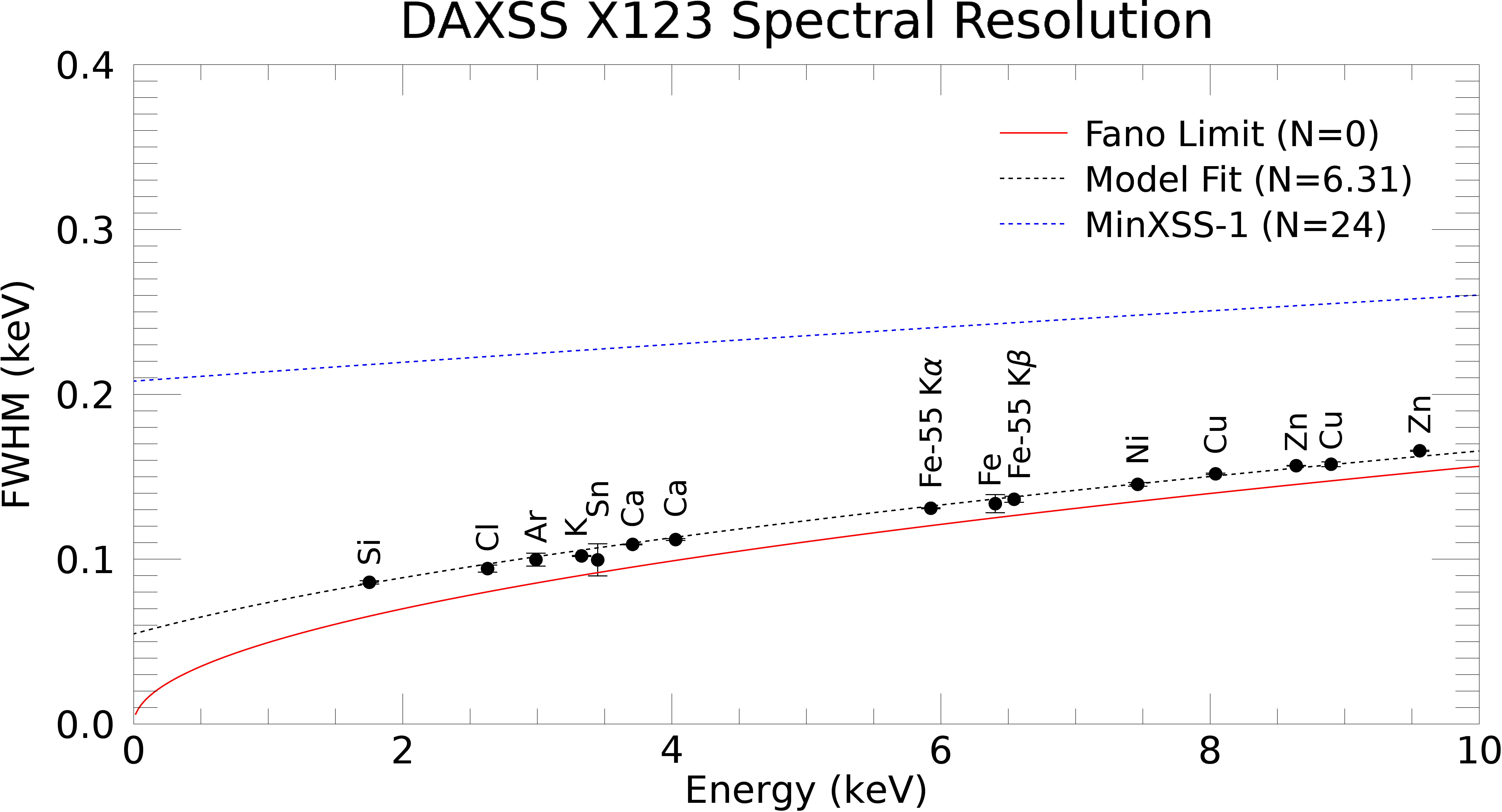
Figure 3: FWHM measurements of X-ray fluorescence from several known sources and the decay products of ⁵⁵Fe. The FWHM of each line was determined by fitting a Gaussian to each emission line and taking the full width of the Gaussian at half of the Gaussian fit’s maximum. The red line indicates the theoretical Fano Noise limit for Si and the dashed black and blue lines are the model fit for the resolution of the DAXSS X-123 FAST SDD detector and the MinXSS-1 X-123, respectively, using Equation 1.

3.3 Linearity of Response

Being a photon-counting detector, it is important to understand DAXSS’s linearity of response with light source intensity. The linearity of the detector was assessed at NIST SURF (Figure 4). Here, all the discussed count rates are the total measured counts across all energy bins during an integration period divided by the time of the integration. Looking at the relationship between the measured count rate and the actual rate provides insight into the severity of dead-time and pile-up effects , the effects of which are described below.

The X-123 FAST SDD has two primary counting channels. The slow counter channel is used to create the X-123 spectrum and has a tunable peaking time (1.2 $\mu$s for DAXSS). The fast counter has a shorter peaking time of 100 ns and an effective pair resolving time of $\sim$120 ns ($\tau_{pair}$, $\tau_{df}$). Because of these features the fast channel operates in anti-coincidence mode with the slow channel. In this way photon peak pile-up events, in which more than one photon is absorbed within the peaking time and recorded as one photon with the sum of the all the photon energies, is minimized but may still occur .

Dead time refers to the time after each measured event during which the instrument cannot record another event. For high ’true’ count rates, losses due to dead time can be significant but the input count rate can still be approximated (Redus et al., 2008; Moore et al., 2018):

$$C_{in}=\frac{C_{f}}{(1-C_{f}\tau_{df})}$$ (2)

where $C_{in}$ represents the ’true’ input count rate, $C_{f}$ is the count rate measured by the fast counter and $\tau_{df}$ is the pair resolving time of the fast counter. From this, the corresponding count rates of the slow counter that are used to generate the spectrum are given by the model:

$$C_{model}=C_{in}e^{-C_{in}\tau_{ds}/2}$$ (3)

where $\tau_{ds}$ is the slow counter dead time. We can see in Figure 4 that this model agrees reasonably well with the NIST SURF with the slow counter dead time found to be $\tau_{ds}=2.875~{}\mu$s. Thus, with the models in Equations 2 and 3 the true count rate during a DAXSS observation can be deduced up to 100,000 counts per second.

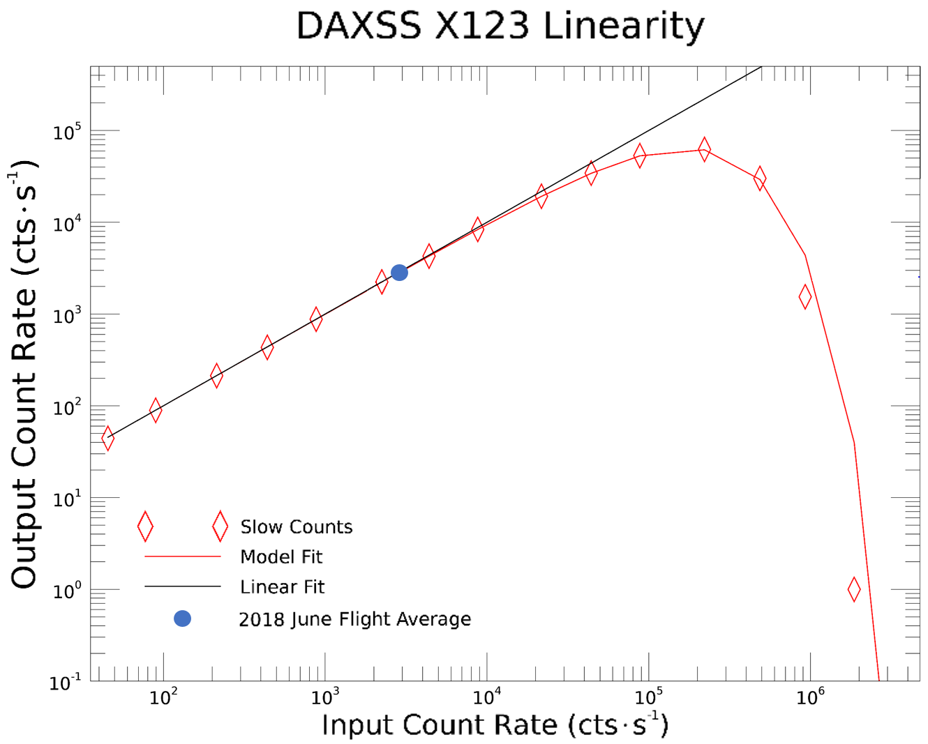
Figure 4: DAXSS detected with 1.2 $\mu$s peaking time. The black line is the linear relationship between the dead time corrected input count rate and the output spectrum count rate. The red line indicates the dead time model fit ($C_{model}$ with $\tau_{ds}=2.875~{}\mu$s) to the measured output count rate ($C_{s}$). The blue dot is the average output count rate seen during the 2018 June rocket flight, given the observed input count rate, which is well below the region in which dead time effects become significant.

3.4 Field of View (FOV) Sensitivity

integrates the incident radiation across its full FOV to create its measured signal. So while DAXSS does not have spatial resolution, its sensitivity does vary slightly with angle of incidence of the incoming solar radiation. The DAXSS front aperture size and distance from the sensor defines a $\pm 4\degree$ clear field of view (FOV). The FOV map obtained from SURF Calibrations indicate a $<$0.5% variance over the $\pm 1\degree$ central FOV. Pointing during the 2018 June rocket flight was maintained well within this central FOV while spectral measurements were being taken.

3.5 Detector Responsivity

The DAXSS instrument spectral efficiency was determined through a series of measurements conducted at NIST SURF. The absolute synchrotron spectral irradiance is used to determine the detection efficiency of the DAXSS instrument. The X-123 count rate per energy bin, , can be calculated by Equation 4 and Equation 5 (Moore et al., 2018):

$$C_{bin,j}=\int_{E_{min},j}^{E_{max},j}\left[\Gamma(E_{det})\right]dE_{det}$$ (4)

$$\Gamma(E_{det})=\int_{0}^{\infty}\int^{\Omega_{\odot}}S(E_{ph},\Omega)\cdot\\ \left[R_{X123}(E_{ph},\Omega,E_{det})\right]d\Omega dE_{ph}$$ (5)

where $S(E_{ph},\Omega)$ is the incoming X-ray signal—depending on the photon energy $E_{ph}$ and the solid angle $\Omega$—and $R_{X123}(E_{ph},\Omega,E_{det})$ is the detected energy bin redistribution function. The energy bin redistribution function maps photon events to detected energy counts which depends on the geometric area and transmission of the each of the two concentric apertures, the detector resolution (Figure 3) and the FOV sensitivity. This mapping can be inverted to take detected counts and create an estimate of the incident photon flux which will be discussed more in Section 4.

$$R_{X123,energy\ bin}=[T_{Be}(E_{ph})A_{small}+\\ T_{both}(A_{large}-A_{small})]R_{Si}(E_{p}h)G(E_{det},E_{ph})$$ (6)

where $T_{Be}$ and $T_{Both}$ are the transmission of beryllium and of both beryllium and Kapton, respectively—calculated using Henke transmission coefficients (Henke et al., 1993), and $A_{small}$ and $A_{large}$ are the geometric areas for the small aperture in the Kapton filter and large aperture in the tungsten cover, respectively. $R_{Si}$ is the responsivity of the X-123 Si diode. $G(E_{det},E_{ph})$ is the redistribution of photon energy to measured energy which can be described as a Gaussian with FWHM from Equation 1.

With the NIST SURF spectra, the relationships described in Equations 4-6, and the spectral resolution fit found in Section 3.2 forward modeling can be done to find a best fit for the only unknowns in our DRA: the sensor Si photopeak response and the filter transmissions of Be and Kapton. The sensor Si thickness, however, affects the energy response more for energies $>$10 keV and did not need to be fitted for the SURF data and as such was assumed to be the thickness provided by Amptek (500 $\mu$m). The SURF synchrotron beam energy is adjustable so that one can calibrate over different energy ranges, with beam energies between 380 MeV and 416 MeV being best for DAXSS calibrations. Fitting this model in Equation 4 to this SURF data, shown in Figure 5, the Kapton thickness is found to be 24.74$\pm$0.04 $\mu$m and the Be thickness is with a reduced $\chi^{2}$ error of 2.48. These effective thicknesses derived from the Henke model are typically different from the physical thickness, but are used self-consistently between calibration and subsequent analysis.

Figure 5: NIST SURF X-ray spectrum measurements from the DAXSS instrument along with model fit described by Equations 4-6.

From the model fit to the NIST SURF spectra in Figure 5 the effective area of DAXSS is found from Equation 6 without the $G(E_{det},E_{ph})$ term.

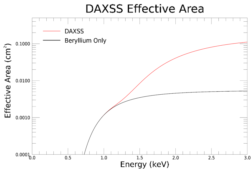
Figure 6: Effective area from the Be contribution compared to that of the full Kapton and Be filter for the DAXSS instrument. Here it is clear to see how the Kapton filter aperture enhances the transmission of photons $\gtrapprox$1.2 keV.

Using the effective area in Figure 6 and the photon redistribution described by a Gaussian with FWHM in Equation 1 the from Equation 6 can be determined. This can now be used with DAXSS solar measurements to estimate the true solar fluxes during observations. This process is described for the 2018 June rocket flight in the following section.

4 Observation and Spectral Model Fits

The DAXSS measurements analyzed here were taken on 2018 June 18 at approximately 19:05 UT over a span of roughly 3.5 minutes. Figure 7 shows an SDO Atmospheric Imaging Assembly (AIA) and Hinode X-ray Telescope (XRT) images from the day of launch.

Figure 7: SDO AIA 193 Å and Hinode XRT images during the 2018 June 18 rocket launch. Two small active regions can be seen near the middle of the solar disk and another behind the east limb. With the absence of large active regions and solar flares, the sun can be classified as being in a quiescent state.

The CHIANTI atomic database, v9.0.1 (Dere et al., 1997, 2019), is used to provide model spectra of solar photon intensity versus energy. This model includes both the continuum and emission lines for given user inputs of solar temperature, emission measure, abundance, and ionization fractions. The default CHIANTI ionization fractions were used for all of the CHIANTI calculations expressed in this paper. Following the process by Caspi et al. (2015), CHIANTI spectra are generated using the IDL SolarSoft function f_vth.pro. This function returns a model solar radiation spectrum as seen at Earth in units of photon flux (photon cm^-2 s^-1 keV^-1). To convert from this output spectrum to detector count rate (counts s^-1) the output model spectrum is multiplied by the response array (units of cm² keV counts photon^-1).

The model spectrum was smoothed to match the energy resolution of DAXSS a direct comparison made to the measured spectrum. The smoothing function that most closely replicates the X-123 detector is a normalized Gaussian function with a full width half maximum (FWHM) that is variable with energy as described in Figure 3. The model spectrum is smoothed by convolving with the Gaussian of variable FWHM. The smoothed model irradiance spectrum in the same units and compatible in energy resolution.

The goodness of fit is characterized quantitatively by finding the reduced $\chi^{2}$ of the model with respect to the measured spectra. The count rate error, or variance array, used for each energy bin in the $\chi^{2}$ calculation assumes standard Poisson counting statistics and is found by taking the square root of the counts in each bin, divided by the integration time.

The fitting region is set to span from 0.7– keV for all of the following model fits. The lower limit is set due to the need for a better detector response model for energies below 0.7 keV as this is where instrumental effects become dominant over the solar signal due to the increasing attenuation of the filter (see Figure 6). This is attributed to excess detector counts due to photon energy-loss processes where higher-energy photons lose some energy before being detected, and hence count as low-energy photons. These processes can include photoelectron emission in the Be window, Si-K escape, Si-L escape, and Compton scattering as theoretically modeled by (Moore et al., 2018), but the specific contributions of these processes have not yet been verified experimentally. The upper limit is due to a low amount of detected photons with energies above  keV which causes a larger amount of photon-counting uncertainty.

In this paper we describe a model that calculates a best fit using one or two temperatures with respective emission measures in addition to a singular , which affects only elements, or a relative AF that varies for each element with emission lines observable above the continuum. The singular AF is a constant that is multiplied by the Feldman standard extended coronal (FSEC) abundance values (Feldman et al., 1992; Landi et al., 2002). The relative AF for each identifiable element is a multiplication factor to the FSEC abundance value for that element while keeping the values for other elements unchanged.

4.1 1T and 2T Models with Single Abundance Factor

The first fit was made assuming the corona was a uniform, plasma a single temperature, single emission measure, and single abundance factor. The parameters were adjusted by an IDL fitting procedure mpfit. This fitting procedure iteratively changes the parameters to find a minimum $\chi^{2}$ value using the Levenberg-Marquardt technique.

Table 1: 1T Fit with Singular AF

	T	EM	AF	Red.Chi-Sq
	(MK)	($${10}^{49}$\ cm^{-3}$)	($\times$ FSEC)
Mean	2.85	0.129	0.91	7.7
Stdev	0.01	0.002	0.01	0.2

Note. — This is a single temperature and single emission measure fit with a singular abundance factor. T represents temperature, EM represents emission measure, and AF represents a singular abundance factor multiplied by Feldman Standard Extended Coronal (FSEC) values (Feldman et al., 1992).

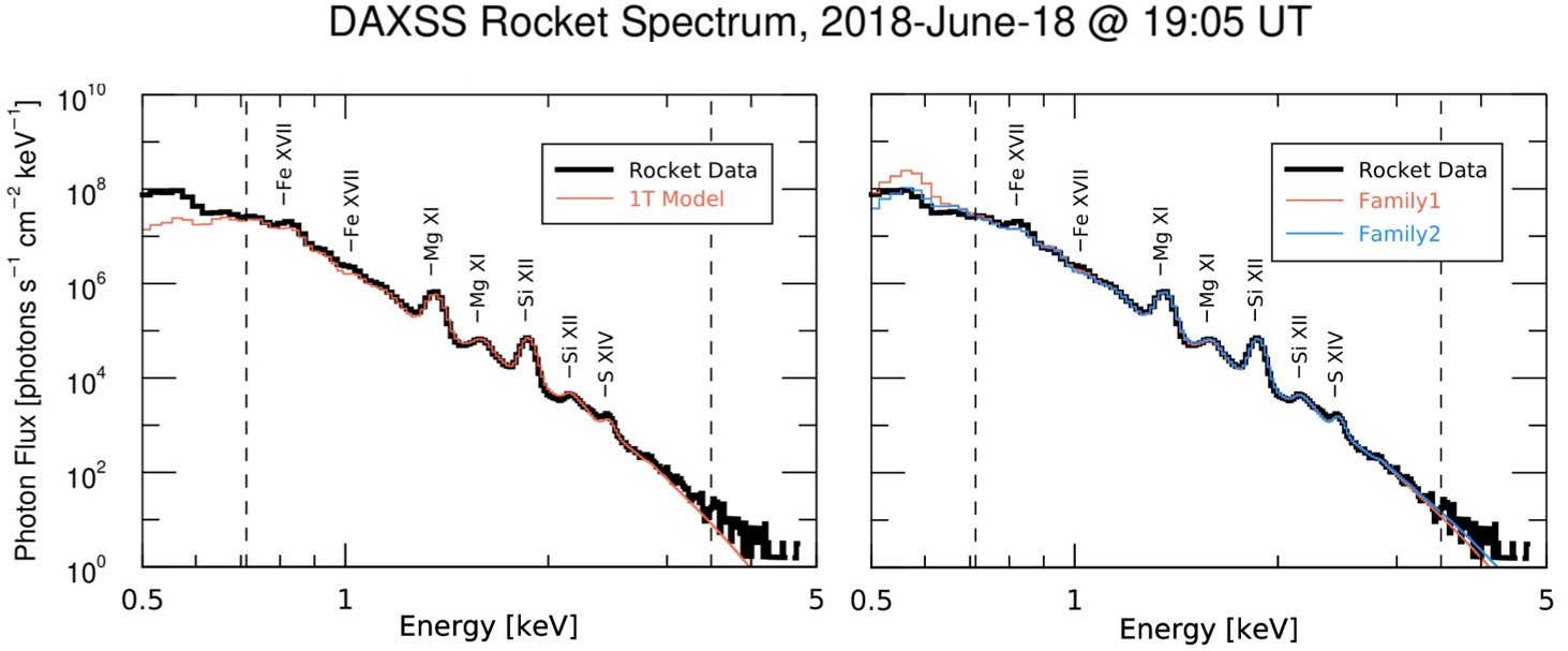
Figure 8: 1T and 2T models with singular AF. Fit range is between 0.7 and 3.5 keV (vertical dashed lines). (Left) 1T model with single temperature, single emission measure, and singular AF. The best-fit parameter values are shown in Table 1. The 1T model is the most simplistic but does not fit well over the whole energy range. (Right) 2T single AF model fit of the flight averaged DAXSS spectrum shows good agreement with the measured data and fits the whole energy range better than a single-temperature model fit. The best-fit parameters for both families are displayed in Table 2

The starts to fall away from the measured data at energies above 2.5 keV. This indicates that there is some coronal plasma at a higher temperature. Therefore, a second fit approach was done to allow for solar plasma at two different temperatures. The same as before, 0.7– keV. This fit has five free parameters to be adjusted: two temperatures, two emission measures, and a single abundance factor. similar $\chi^{2}$ goodness of fit

Figure 8 (Right) shows the model produced by each family of best-fit values. The fit follows the measured spectra more closely into higher energies while maintaining a good fit at the lower energies as well. The reduced $\chi^{2}$ value using the fitting method decreased to indicating a closer model fit to the DAXSS measurement. There is a visible disagreement between the modeled and measured spectra at around 0.82 keV. The explanations to this discrepancy are discussed in the conclusion (Sec. 6).

4.2 2T Multiple AF Model

The parameters found in the fits for temperature and emission measure can be passed back into CHIANTI to produce a line list of ions contributing to spectrum. This line list allows us to calculate the estimated elemental emission contribution to each of the blended lines we see in the rocket measurement, as shown in Table 3. From this it is evident that the line features seen in the DAXSS spectra are dominated by Mg, Si, S, and Fe using this CHIANTI line list.

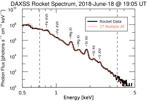
Figure 9: 2T multiple AF model fit with variable parameter abundances of four identifiable low-FIP elements: Mg, Si, S, and Fe. Fit range is between 0.7 and 3.5 keV (vertical dashed lines). This 2T multiple AF model shows the best agreement with the measured DAXSS data. The best-fit parameter values are reported in Table 4.

As such, in a third fit, shown in Figure 9, the relative abundances of the four low-FIP elements Mg, Si, S, and Fe are made to be free parameters in addition to two temperatures and their respective emission measures. The addition of individual abundance factors for each identifiable element in the DAXSS spectrum can account for the abundances in the corona deviating from FSEC abundance values. One thousand iterations of this fitting process was also done only a single family of parameters was found. The relative abundances that give the lowest $\chi^{2}$ fit and therefore the best fit are listed in Table 4.

Table 2: DAXSS Solar SXR Model Measurements with Singular Abundance Factor

	T1	EM1	T2	EM2	AF	Red.Chi-Sq	Percentage
	(MK)	($${10}^{49}$\ cm^{-3}$)	(MK)	($${10}^{49}$\ cm^{-}3$)	($\times$ FSEC)		($\%$)
Family 1 Mean	1.59	1.11	3.14	0.061	1.07	4.5	48.9
Family 1 Stdev	0.01	0.04	0.02	0.002	0.01	0.2	$\cdots$
Family 2 Mean	2.10	0.35	3.48	0.026	1.02	4.9	50.3
Family 2 Stdev	0.01	0.01	0.04	0.002	0.01	0.2	$\cdots$

Note. — This is a two temperature and two emission measure fit with a singular abundance factor. T represents temperature, EM represents emission measure, and AF represents a singular abundance factor multiplied by Feldman Standard Extended Coronal (FSEC) values (Feldman et al., 1992). The percentage column represents the number of iterations out of 1,000 that showed up in each family.

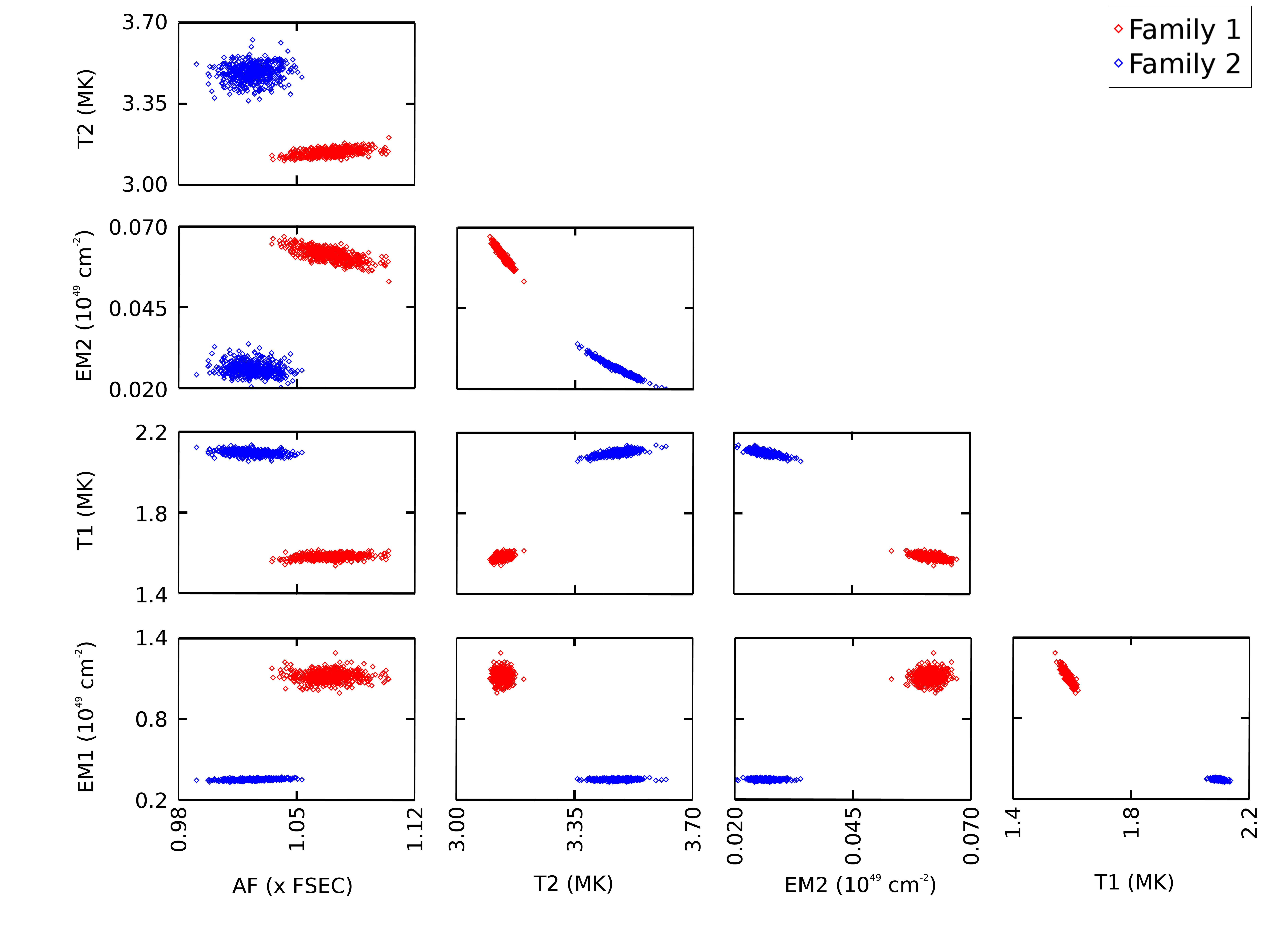
Figure 10:

Table 3: Leading Elemental and Ion Emission Contributions to Peak Features in 2018 Jun. 18 DAXSS Spectra.

Peak Location	Primary	Secondary
(keV)	(%)	(%)
0.81	Fe: 90.19 (XVII, XVI)	O: 9.11 (VIII)
0.91	Ne: 88.42 (IX, VII)	Fe: 8.16 (XVII)
1.01	Fe: 63.67 (XVII)	Ne: 27.30 (X, IX)
1.35	Mg: 98.83 (XI, X)	$\cdots$
1.57	Mg: 66.96 (XI, X)	Al: 32.01 (XII)
1.85	Si: 98.83 (XII, XIII)	Al: 1.12 (XI)
2.13	Si: 99.42 (XII, XIII)	$\cdots$
2.43	S: 99.97 (XIV, XV)	$\cdots$

Note. — CHIANTI spectral parameters of $T_{1}=2.10\ MK$ and $T_{2}=3.48\ MK$ with $EM_{1}=$0.35\text{\times}{10}^{49}$\ cm^{-3}$ and $EM_{2}=$0.026\text{\times}{10}^{49}$\ cm^{-3}$ with FSEC abundance. Elements only listed if contributing $\geq$1%.

Table 4: DAXSS Solar SXR Model Measurements with Abundance Factor for Identifiable Elements

	T1	EM1	T2	EM2	Mg AF	Si AF	S AF	Fe AF	Red.Chi-Sq
	(MK)	($${10}^{49}$\ cm^{-3}$)	(MK)	($${10}^{49}$\ cm^{-}3$)	($\times$ FSEC)	($\times$ FSEC)	($\times$ FSEC)	($\times$ FSEC)
Mean	1.86	0.50	3.29	0.043	1.02	0.99	1.00	1.35	3.9
Stdev	0.02	0.02	0.03	0.003	0.01	0.02	0.05	0.02	0.2

Note. — These values are from a two temperature and two emission measure fit with a separate abundance factor for each identifiable element in the DAXSS spectrum. T represents temperature, EM represents emission measure, and AF represents an abundance factor for each element multiplied by its respective Feldman Standard Extended Coronal (FSEC) value (Feldman et al., 1992). All other FSEC abundance values are maintained as their original value.

The relative for Mg, Si, and S are all within 2 percent of their FSEC abundance values. The relative of Fe, however, was found to be percent higher than its FSEC abundance value. When adding more free parameters to a model it is expected that the reduced $\chi^{2}$ will decrease, but there is also a risk that the model strays further from physical reality. This discrepancy and feature is further discussed in the conclusion (Sec. 6).

5 Comparisons

5.1 Previous SXR Measurements

The 2018 June 18 DAXSS rocket measurement can be validated by other solar SXR observations. From Figure 11 one can see that MinXSS-1 measurements, from similar solar conditions, and derived SXR spectra from simultaneous EVE MEGS-A EUV measurements have very similar spectra as the DAXSS measurement. Additionally, from Table 5 one can see that models, derived during similar solar conditions, yield similar results to those described in Sec.4, more so for the lower temperature component. Notably, the SphinX measurement at lower solar activity has a cooler temperature and lower emission measure than the DAXSS measurement. Furthermore, there are hotter temperatures for the more active measurements in 2003 and 2012.

Figure 11: Comparisons from other Si-diode spectrometer measurements to the 2018 June 18 DAXSS rocket flight (solar activity levels and spectral fitting for each spectra shown in Table 5). The EVE spectrum is created by deriving a DEM from the rocket EVE’s Multiple Extreme ultraviolet Grating Spectrograph (MEGS-A: 6-37 nm) spectral observation during the rocket flight (Subsec. 5.2), and this DEM is then used in CHIANTI to generate a SXR spectrum at the resolution of DAXSS.

From Table 6 and Figure 11 it is shown that DAXSS offers significantly improved energy resolution in the SXR spectrum compared to the previous photon-counting Si-diode SXR spectrometers and thus can better spectrally resolve and identify some elemental line features. As shown in Figure 3, the resolution varies with energy, and the DAXSS resolution is about three times better than MinXSS-1 at the lower energy (1 keV) and about 50% better at higher energy (10 keV). Crystal spectrometers, such as the Bragg Crystal Spectrometer (BCS) on Yohkoh (Švestka & Uchida, 1991) and CORONAS/RESIK (Sylwester et al., 1998) and the Bent Crystal Spectrometer on the Solar Maximum Mission (SMM) (Acton et al., 1980), offer much higher spectral resolution than seen on Si-diode spectrometers and as such can offer absolute abundance measurements over their narrow passbands. For example, the Yohkoh BCS observes the S XV emission over 5.02 – 5.11 Å (2.5 keV) and the Ca XIX emission over 3.16 – 3.20 Å (3.9 keV) (Culhane, 1996). However, as DAXSS has a wider passband, and improved resolution from previous Si-diode instruments, it has the benefit of making simultaneous inferred abundance measurements from multiple elements, as well as temperature and emission measure measurements (as done in Subsec. 4.2). Furthermore, measurements from these previous crystal spectrometers did not observe elemental lines below $\sim$2.4 keV, meaning that DAXSS can provide improved insight into abundance, temperature, and emission measure models for the SXR between 0.5 – 2.5 keV.

5.2 DEM Comparisons

Comparison of the DAXSS two-temperature (2T) model fits to differential emission measure (DEM) estimates from other instruments could help validate the DAXSS simple modeling approach. Moore et al. (2018) shows that the X123 response is primarily over the temperature range of 1 MK to 10 MK, so this comparison needs to be done over a similar range, such as is accessible with using DEMs derived from extreme ultraviolet (EUV) emissions. One of the comparison is with the DEM derived with Solar Dynamics Observatory (SDO) Extreme ultraviolet Variability Experiment (EVE) solar EUV spectral irradiance data in the 6 nm to 37 nm range. The derivation of EVE-based DEM estimates is being developed for improving the X-ray ultraviolet Photometer System (XPS) data processing for the Solar Radiation and Climate Experiment (SORCE) and Thermosphere, Ionosphere, Mesosphere, Energetics, and Dynamics (TIMED) missions. The primary DEMs for this analysis is the quiet sun (QS) and active region (AR) DEMs as needed for estimating the daily variations of the solar XUV spectral irradiance for the XPS Level 4 product (Woods et al., 2008). The Fe VIII to Fe XVI lines in the SDO EVE spectra were initially used to estimate the DEMs for the reference QS and AR spectra derived with EVE data between 2010 and 2013 using the technique described by Schonfeld et al. (2017). It was then found that fitting with DEM Gaussian profiles with logarithmic Temperature (K, log(T)) peaks every 0.2 and with Gaussian width of 0.42 in log(T) (FWHM of 1.0) provided more robust solutions for the DEM (similar technique described by Warren et al. (2013)). Furthermore, fitting just specific Fe lines was providing low irradiance estimates in the 6 nm to 15 nm range. Better spectral model values for this range was found when fitting the EVE spectra over the ranges of 10 to 14 nm and 26 to 30 nm. The DEM estimate using just the rocket EVE spectral data flown with DAXSS on 2018 June 18 and the DEM based on combining the QS DEM and the AR DEM with an AR scaling factor of 0.00806 are shown in Figure 12. This scaling factor for the AR EM was determined as the best fit for the DAXSS spectral irradiance. The conversion of the EVE-based DEM ($cm^{-5}K^{-1}$) to EM ($cm^{-3}$) for comparison to DAXSS 2T solution is the multiplication by the solar hemisphere area ($$3.04\text{\times}{10}^{22}$cm^{2}$) and by the temperature bin size (0.23 * Temperature in K).

The DAXSS family of 2T solutions for the SXR range have very similar emission measures (EM) profile over temperature as derived from the EVE data in the EUV range, but the DAXSS EM values are a factor of higher. Most of this difference is because the DAXSS 2T solution is only at two temperatures whereas the EVE result is a DEM over many temperatures. The difference between the EVE model EM and an iso-thermal EM is estimated to be about a factor of 4. However, some of this difference can be attributed to the DAXSS 2T solutions having a lower abundance factor than the Feldman et al. (1992) abundance values used in CHIANTI for the EVE-based DEM modeling (Feldman et al., 1992). The 10 percent decrease in the abundance factor for the DAXSS 2T solution does increase its EM relative to an EM result using the standard (unadjusted) Feldman et al. (1992) abundance values used in CHIANTI for the EVE-based DEM modeling. It is most important to note that the DAXSS 2T model results with multiple solutions (families) appear to all be valid solutions because they follow the same profile over temperature as the EVE-based DEM model results.

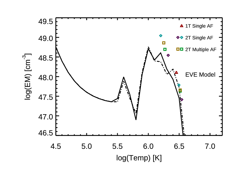
Figure 12: Comparison of DAXSS 1T Single AF model (Table 1, triangle), 2T Single AF model (Table 2, diamonds) and 2T multiple AF model (Table 4, squares) to rocket EVE-derived EM results (black solid line). The EVE-based DEM model with QS and AR DEMs is the dot-dashed line.

5.3 Validation for GOES XRS

The rocket DAXSS calibrated SXR spectral irradiance also provides a validation for the new generation of the X-Ray Sensor $XRS$ aboard the GOES-16 and GOES-17 operational satellites (Goodman et al., 2020). assumes a flat spectrum, that is, no wavelength variation for $E_{ref}$. As listed in Table 7, the GOES-16 and GOES-17 solar irradiance Level 2, $E_{L2}$, values for the 1-8 Å XRS-B channel are $6.18\text{\times}{10}^{-8}$ $\mathrm{W}\text{\,}{\mathrm{m}}^{-2}$ and $6.67\text{\times}{10}^{-8}$ $\mathrm{W}\text{\,}{\mathrm{m}}^{-2}$  respectively .

The DAXSS irradiance integrated over the XRS-B 1-8 Å band is $4.59\text{\times}{10}^{-8}$ $\mathrm{W}\text{\,}{\mathrm{m}}^{-2}$. solar spectrum instrument spectral responsivity, R provide a predicted XRS of 0.81 pA and 0.83 pA for GOES-16 and 17, respectively. Then comparison of these predicted signals to the measured XRS signals provides more accurate irradiance results (Equation 10) from GOES-16 and 17 XRS-B of $5.17\text{\times}{10}^{-8}$ $\mathrm{W}\text{\,}{\mathrm{m}}^{-2}$ and $5.45\text{\times}{10}^{-8}$ $\mathrm{W}\text{\,}{\mathrm{m}}^{-2}$, respectively. These are 13% and 19% higher than the DAXSS 1-8 Å irradiance.

$$I_{measure}=E_{L2}\cdot R_{integ}$$ (7)

$$R_{integ}=\frac{\int_{0}^{\infty}R(\lambda)\cdot A\cdot E_{ref}(\lambda)\cdot d\lambda}{\int_{\lambda_{1}}^{\lambda_{2}}E_{ref}(\lambda)\cdot d\lambda}$$ (8)

$$I_{predict}=\int_{0}^{\infty}R(\lambda)\cdot A\cdot E_{DAXSS}(\lambda)\cdot d\lambda$$ (9)

$$E_{XRS_{true}}=\frac{I_{measure}}{I_{predict}}\cdot E_{DAXSS}$$ (10)

Table 5: Solar temperature and emission measure comparisons during quiet or non-flaring solar activity.

Observation	P10 Index	Observatory	Temperature 1	Emission Measure 1	Temperature 2	Emission Measure 2
(YYYY-MM-DD)	(s.f.u.)		($\log$ MK)	($${10}^{49}$\ cm^{-3}$)	($\log$ MK)	($${10}^{49}$\ cm^{-3}$)
2018-06-18	75.14	NASA 36.336 (DAXSS)α	1.56	1.13	3.08	0.068
2016-11-21 – 2016-11-22	75.19	MinXSS-1β	2.36	0.28	5.00	0.008
2012-06-23 (Caspi et al., 2015)	112.91	NASA 36.286	2.9	0.49	11	0.0014
2009-09-16 (Sylwester et al., 2012)	70.28	SphinX	1.71	0.0978	$\cdots$	$\cdots$
2003 (Sylwester et al., 2010)	$\cdots$	RESIKγ	2.9	0.17	9.1	0.023

Note. — ^αDAXSS measurement from Family 1 in Table 2. ^βMinXSS-1 measurements are determined by fitting two temperatures and EMs over the spectrum from 0.9–2.7 keV. ^γAveraged data taken from early 2003 when GOES levels were between A9 – B1. P10 index is defined as the average of the F10.7 cm radio flux and 80-day smoothed F10.7 cm radio flux.

Table 6: Resolution Comparison of Wide Passband Spectrometers

Instrument	Resolution (keV)	Energy (keV)
DAXSS	0.069 – 0.228	0.7 – 20
MinXSS-1	0.214 – 0.341	1.0 – 30
CORONAS-PHOTON/SphinX (Sylwester et al., 2012)	0.464α	1.2 – 14.9
MESSENGER/SAX (Dennis et al., 2015)	0.6	6
GSAT-2/SOXS (Jain et al., 2006)	0.7	6

Note. — ^αSphinX resolution quoted as the same over its entire passband.

Table 7: GOES XRS comparison to DAXSS

	GOES-16	GOES-17
	XRS-B: 1-8 Å	XRS-B: 1-8 Å
$E_{L2}:$ NOAA-reported XRS L2 Irradiance (W/m2)	$$6.18\text{\times}{10}^{-8}$\ \pm\ $0.3\text{\times}{10}^{-8}$$	$$6.67\text{\times}{10}^{-8}$\ \pm\ $0.4\text{\times}{10}^{-8}$$
$R_{integ}:$ XRS Response Integrated (A/(W/m2))	$9.615\text{\times}{10}^{-6}$	$9.577\text{\times}{10}^{-6}$
$I_{measure}:$ XRS Sensor Current Measured (A)	$9.07\text{\times}{10}^{-13}$	$9.86\text{\times}{10}^{-13}$
$I_{predict}:$ XRS Sensor Current Predicted (A)	$8.05\text{\times}{10}^{-13}$	$8.30\text{\times}{10}^{-13}$
DAXSS $1-8\AA$ Irradiance (W/m2)	$$4.59\text{\times}{10}^{-8}$\ \pm\ $0.46\text{\times}{10}^{-8}$$	$$4.59\text{\times}{10}^{-8}$\ \pm\ $0.46\text{\times}{10}^{-8}$$
$E_{XRS_{true}}:$ XRS ”True” Irradiance (W/m2)	$$5.17\text{\times}{10}^{-8}$\ \pm\ $0.8\text{\times}{10}^{-8}$$	$$5.45\text{\times}{10}^{-8}$\ \pm\ $0.8\text{\times}{10}^{-8}$$
Ratio (DAXSS Irrad./GOES ”True” Irrad.)	$0.89\ \pm\ 0.16$	$0.84\ \pm\ 0.16$

Considering about 10% accuracy for each instrument responsivity as DAXSS and GOES XRS instruments were each calibrated at SURF using similar techniques, the 1-sigma uncertainty for this comparison is estimated to be 18%. While the XRS difference to DAXSS is close to this 1-sigma uncertainty, we suspect that the XRS signals could still have a particle (energetic electrons) background signal contribution, which is a known concern for the GOES solar observations in its GEO orbit. The GOES-16 and 17 XRSs have been cross-calibrated to agree at higher flare irradiance levels, so the 5% difference between GOES-16 and GOES-17 for this comparison at low solar activity is also suggestive that their corrections for particle background signals could be improved. The flight of DAXSS-2 in 2021 on the EVE calibration rocket will provide additional validation for the GOES XRS. If this 2021 flight is during a period of higher solar activity (as expected for solar cycle 25), then we anticipate a more accurate comparison from having larger signals (higher signal-to-noise), and also a validation for the XRS-A 0.5-4 Å channel could be possible.

6 Conclusions

The DAXSS instrument with the Amptek X-123 FAST SDD spectrometer provides improved measuring capabilities in the soft X-ray regime than previous flights of X123-type technology. The latest rocket spectrum has better energy resolution by more than a factor of two and improved sensitivity over a wider energy range than its previous flights because of the improvements that Amptek has made to the X-123 and due to the dual-zone aperture design for DAXSS. These improvements allow DAXSS to better fill a long-standing gap in the SXR region of solar observations with more detailed information. The measurements from DAXSS show lines with improved spectral resolution, compared to prior Si photodiode measurements, allowing for improved coronal temperature and emission measure models, as well as the ability to more accurately fit abundances per individual element.

A two-temperature (2T) model was fit to the measured rocket DAXSS spectrum and a lower $\chi^{2}$ value, than a single temperature . 2T model agree with the measured data from lower photon energies of 0.7 keV out to higher energies of  keV. the 2T model temperatures and emission measures are also consistent with the EVE-derived DEM profiles.

The 2T model fit included both a fit for a singular abundance factor and with multiple abundance factors for some select elements. For , the resulting AF was seen in Table 4. the abundance of iron was found to be percent higher than the currently accepted FSEC abundance value for quiescent sun.

The model that we are using, which only includes two temperatures and two emission measures, could be insufficient for modeling the solar spectrum and may not accurately represent the temperature contributions in this region of the spectrum. This would lead to incorrect line-to-continuum ratios and improper abundance values. Creating a DEM model based on the DAXSS spectrum might clear up this possibility. Another explanation for this large discrepancy in the abundance of iron could be that there are missing elemental emission lines in the CHIANTI line database near those energies, which then are not represented in its modeled solar spectrum. It could also be that there is a higher abundance of the element emitting at 0.82 keV than the FSEC abundances, although this would go against many prior measurements including in the EUV and X-rays. To resolve the discrepancy whether the excess flux is a legitimate measurement or due to a simplistic model, or the need for updated spectral fitting or atomic modeling, we need additional high-resolution, high-sensitivity long-term systematic measurements from instruments in this energy range in the future.

There is on-going work to improve the instrument response model at energies below 0.7 keV. At those lower energies, the X-123 response is affected greatly by the photoelectric effect on its Be filter, Si-K escape, Si-L escape, and Compton scattering causing diversion away from the simplified response model based directly on the NIST SURF calibrations. Future differential emission measure (DEM) analysis is also planned in order to obtain more complete temperature coverage, and will include SDO and Hinode observations to expand the temperature coverage even further.

Sounding rocket flights are a great platform to demonstrate new technology, such as the DAXSS instrument, as well as to investigate the properties of the sun on a particular day. Daily observations over several years are needed to achieve for how the coronal heating processes, plasma temperature, and composition change for active regions during different solar cycle phases, and higher cadence observations of the order of a few seconds are needed for flare energetics studies. The rocket DAXSS instrument is being prepared for a flight of opportunity on the InspireSat-1 with its launch planned for late 2020. This flight will provide science data needed by solar physicists to study solar active region evolution and flare energetics and to provide evidence that discriminates between competing models of coronal heating through detailed analysis of the solar SXR spectra.

References

- Acton et al. (1980) Acton, L. W., Culhane, J. L., Gabriel, A. H., et al. 1980, Solar Physics, 65, 53, doi: 10.1007/bf00151384
- Amptek (2020) Amptek. 2020, AN-DPP-002: Operating the DP5 At High Rates. https://www.amptek.com/-/media/ametekamptek/documents/resources/andpp2.pdf
- Arp et al. (2011) Arp, U., Clark, C., Deng, L., et al. 2011, Nuclear Instruments and Methods in Physics Research Section A: Accelerators, Spectrometers, Detectors and Associated Equipment, 649, 12–14, doi: 10.1016/j.nima.2010.11.078
- Asgari-Targhi & Ballegooijen (2012) Asgari-Targhi, M., & Ballegooijen, A. A. V. 2012, The Astrophysical Journal, 746, 2, doi: 10.1088/0004-637X/746/1/81
- Caspi et al. (2015) Caspi, A., Woods, T. N., & Warren, H. P. 2015, The Astrophysical Journal, 802, doi: 10.1088/2041-8205/802/1/l2
- Culhane (1996) Culhane, J. L. 1996, in Astronomical Society of the Pacific Conference Series, Vol. 109, Cool Stars, Stellar Systems, and the Sun, ed. R. Pallavicini & A. K. Dupree, 188–192
- Dennis et al. (2015) Dennis, B. R., Phillips, K. J. H., Schwartz, R. A., et al. 2015, The Astrophysical Journal, 803, 67, doi: 10.1088/0004-637x/803/2/67
- Dere et al. (2019) Dere, K. P., Del Zanna, G., Young, P. R., Landi, E., & Sutherland, R. S. 2019, The Astrophysical Journal Supplement Series, 241, 9, doi: https://doi.org/10.3847/1538-4365/ab05cf
- Dere et al. (1997) Dere, K. P., Landi, E., Mason, H. E., Fossi, B. C. M., & Young, P. R. 1997, Astronomy and Astrophysics Supplement Series, 125, 149–173, doi: 10.1051/aas:1997368
- Feldman et al. (1992) Feldman, U., Mandelbaum, P., Seely, J. F., Doschek, G. A., & Gursky, H. 1992, ApJS, 81, 387, doi: 10.1086/191698
- Fletcher et al. (2011) Fletcher, L., Dennis, B. R., Hudson, H. S., et al. 2011, Space Science Reviews, 159, 19, doi: 10.1007/s11214-010-9701-8
- Golub & Pasachoff (2010) Golub, L., & Pasachoff, J. M. 2010, The solar corona (Cambridge University Press)
- Goodman et al. (2020) Goodman, S., Schmit, T. J., Daniels, J. M., & Redmond, R. J. 2020, The GOES-R series: a new generation of geostationary environmental satellites (Elsevier), 233–242
- Henke et al. (1993) Henke, B., Gullikson, E., & Davis, J. 1993, Atomic Data and Nuclear Data Tables; (United States), doi: 10.1006/adnd.1993.1013
- Hock et al. (2012) Hock, R. A., Chamberlin, P. C., Woods, T. N., et al. 2012, Solar Physics, 275, 145, doi: 10.1007/s11207-010-9520-9
- Jain et al. (2006) Jain, R., Joshi, V., Kayasth, S. L., Dave, H., & Deshpande, M. R. 2006, Journal of Astrophysics and Astronomy, 27, 175, doi: 10.1007/bf02702520
- Klimchuk (2006) Klimchuk, J. A. 2006, Solar Physics, 234, 41–77, doi: 10.1007/s11207-006-0055-z
- Knoll (2000) Knoll, G. F. 2000, Radiation detection and measurement (Wiley)
- Laming (2015) Laming, J. M. 2015, Living Reviews in Solar Physics, 12, doi: 10.1007/lrsp-2015-2
- Landi et al. (2002) Landi, E., Feldman, U., & Dere, K. P. 2002, The Astrophysical Journal, 574, 495, doi: 10.1086/340837
- Lin et al. (2002) Lin, R., Dennis, B., Hurford, G., et al. 2002, Solar Physics, 210, 3, doi: 10.1023/a:1022428818870
- Mariska (2006) Mariska, J. T. 2006, The Astrophysical Journal, 639, 485, doi: https://doi.org/10.1086/499296
- Mason et al. (2016) Mason, J. P., Woods, T. N., Caspi, A., et al. 2016, Journal of Spacecraft and Rockets, 53, 328–339, doi: 10.2514/1.a33351
- Mason et al. (2019) Mason, J. P., Woods, T. N., Chamberlin, P. C., et al. 2019, Advances in Space Research, doi: 10.1016/j.asr.2019.02.011
- McTiernan (2009) McTiernan, J. 2009, The Astrophysical Journal, 697, 94, doi: 10.1088/0004-637X/697/1/94
- Moore et al. (2018) Moore, C. S., Caspi, A., Woods, T. N., et al. 2018, Solar Physics, 293, doi: 10.1007/s11207-018-1243-3
- Parker (1988) Parker, E. N. 1988, The Astrophysical Journal, 330, 474, doi: 10.1086/166485
- Pesnell et al. (2012) Pesnell, W., Thompson, B., & Chamberlin, P. 2012, Solar Physics, 275, 3, doi: https://doi.org/10.1007/s11207-011-9841-3
- Pesnell et al. (2011) Pesnell, W. D., Thompson, B. J., & Chamberlin, P. C. 2011, Solar Physics, 275, 3–15, doi: 10.1007/s11207-011-9841-3
- Redus et al. (2008) Redus, R., Huber, A., & Sperry, D. 2008, IEEE Nuclear Science Symposium Conference Record, 3416 , doi: 10.1109/NSSMIC.2008.4775075
- Schonfeld et al. (2017) Schonfeld, S. J., White, S. M., Hock-Mysliwiec, R. A., & Mcateer, R. T. J. 2017, The Astrophysical Journal, 844, 163, doi: 10.3847/1538-4357/aa7b35
- Smith (2003) Smith, D. M. 2003, The Astrophysical Journal, 589, 55, doi: https://doi.org/10.1086/375795
- Su et al. (2018) Su, Y., Veronig, A. M., Hannah, I. G., et al. 2018, The Astrophysical Journal, 856, L17, doi: 10.3847/2041-8213/aab436
- Sylwester et al. (2010) Sylwester, B., Sylwester, J., & Phillips, K. 2010, Astronomy and Astrophysics, 514, doi: 10.1051/0004-6361/200912907
- Sylwester et al. (1998) Sylwester, J., Gaicki, I., Kordylewski, Z., et al. 1998, in ESA Special Publication, Vol. 417, Crossroads for European Solar and Heliospheric Physics. Recent Achievements and Future Mission Possibilities, 313
- Sylwester et al. (2012) Sylwester, J., Kowalinski, M., Gburek, S., et al. 2012, The Astrophysical Journal, 751, 111, doi: 10.1088/0004-637x/751/2/111
- Švestka & Uchida (1991) Švestka, Z., & Uchida, Y. 1991, The Yohkoh (Solar-A) Mission (Springer Netherlands), 4
- Warren (2014) Warren, H. P. 2014, The Astrophysical Journal Letters, 786, 6, doi: https://doi.org/10.1088/2041-8205/786/1/L2
- Warren et al. (2013) Warren, H. P., Mariska, J. T., & Doschek, G. A. 2013, The Astrophysical Journal, 770, 116, doi: 10.1088/0004-637x/770/2/116
- Woods et al. (2017) Woods, T., Caspi, A., Chamberlin, P., et al. 2017, The Astrophysical Journal, 835, 122, doi: 10.3847/1538-4357/835/2/122
- Woods (2005) Woods, T. N. 2005, Journal of Geophysical Research, 110, doi: 10.1029/2004ja010765
- Woods et al. (2005) Woods, T. N., Rottman, G., & Vest, R. 2005, Solar Physics, 230, 345, doi: 10.1007/s11207-005-4119-2
- Woods et al. (2008) Woods, T. N., Chamberlin, P. C., Peterson, W. K., et al. 2008, Solar Physics, 250, 235–267, doi: 10.1007/s11207-008-9196-6
- Woods et al. (2012) Woods, T. N., Eparvier, F. G., Hock, R., et al. 2012, Solar Physics, 275, 115, doi: 10.1007/s11207-009-9487-6