Likelihood Landscapes: A Unifying Principle Behind Many Adversarial Defenses

Abstract

Convolutional Neural Networks have been shown to be vulnerable to adversarial examples, which are known to locate in subspaces close to where normal data lies but are not naturally occurring and of low probability. In this work, we investigate the potential effect defense techniques have on the geometry of the likelihood landscape - likelihood of the input images under the trained model. We first propose a way to visualize the likelihood landscape leveraging an energy-based model interpretation of discriminative classifiers. Then we introduce a measure to quantify the flatness of the likelihood landscape. We observe that a subset of adversarial defense techniques results in a similar effect of flattening the likelihood landscape. We further explore directly regularizing towards a flat landscape for adversarial robustness.

1 Introduction

Although Convolutional Neural Networks (CNNs) have consistently pushed benchmarks on several computer vision tasks, ranging from image classification [15], object detection [8] to recent multimodal tasks such as visual question answering [1] and dialog [3], they are not robust to small adversarial input perturbations. Prior work has extensively demonstrated the vulnerability of CNNs to adversarial attacks [39, 10, 29, 2, 24] and has therefore, exposed how intrinsically unstable these systems are. Countering the susceptibility of CNNs to such attacks has motivated a number of defenses in the computer vision literature [24, 49, 43, 27, 16, 18, 35, 33].

In this work we explore the questions, why are neural networks vulnerable to adversarial attacks in the first place, and how do adversarial defenses protect against them? Are there some inherent deficiencies in vanilla neural network training that these attacks exploit and that these defenses counter? To start answering these questions, we explore how adversarial and clean samples fit into the marginal input distributions of trained models. In doing so, we find that although CNN classifiers implicitly model the distribution of the clean data (both training and test), standard training induces a specific structure in this marginal distribution that adversarial attacks can exploit. Moreover, we find that a subset of adversarial defense techniques, despite being wildly different in motivation and implementation, all tend to modify this structure, leading to more robust models.

A standard discriminative CNN-based classifier only explicitly models the conditional distribution of the output classes with respect to the input image (namely, $p_{\theta}(y|x)$). This is in contrast to generative models (such as GANs [9]), which go a step further and model the marginal (or joint) distribution of the data directly (namely, $p_{\theta}(x)$ or $p_{\theta}(x,y)$), so that they can draw new samples from that distribution or explain existing samples under the learned model. Recently, however, Grathwohl et al. [12] have shown that it is possible to interpret a CNN classifier as an energy-based model (EBM), allowing us to infer the conditional ($p_{\theta}(y|x)$) as well as the marginal distribution ($p_{\theta}(x)$). While they use this trick to encode generative capabilities into a discriminative classifier, we are interested in exploring the marginal distribution of the input, $p_{\theta}(x)$ for models trained with and without adversarial defense mechanisms.

To do this, we study the “relative likelihood landscape” ($\Delta\log p_{\theta}(x)$ in a neighborhood around a test example), which lets us freely analyze this marginal distribution. In doing so, we notice a worrying trend – for most training or test examples, a small random perturbation in pixel space can cause the modeled $\log p_{\theta}(x)$ to drop significantly (see Fig. 1a). Despite training and test samples (predicted correctly by the model) being highly likely under the marginal data distribution of the model (high $\log p_{\theta}(x)$), slight deviations from these examples significantly moves the perturbed samples out of the high-likelihood region. Whether this is because of dataset biases such as chromatic aberration [4] and JPEG artifacts [38] or some other factor [40, 6, 17] isn’t clear. Yet, what is clear is that adversarial examples exploit this property (see Fig. 3a). Moreover, we observe that adversarial defenses intrinsically address this issue.

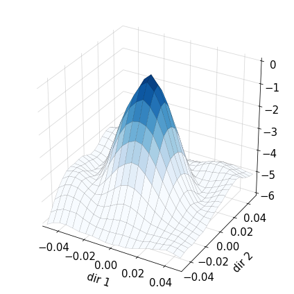
(a) Standard training

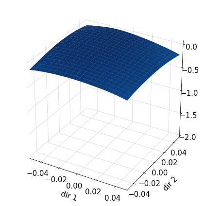
(b) Adv Training, $\epsilon=6$

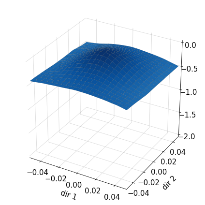
(c) Jacobian Reg, $\lambda=0.05$

Figure 1: Relative likelihood landscapes $(\Delta\log p_{\theta}(x))$ plotted over two random perturbation directions for three DDNet models trained on CIFAR10 with the clean sample in the center. (a) follows standard training without additional defense. (b) uses PGD based adversarial training for 10 iterations with $\epsilon=6/255$. (c) uses Jacobian regularization with a strength of $\lambda=0.05$. Models trained to defend against adversarial attacks tend to have much fatter landscapes.

Specifically, we study two key adversarial defense techniques – namely adversarial training [10, 24, 49] and Jacobian regularization [18, 16]. Although these defense mechanisms are motivated by different objectives, both of them result in elevating the value of $\log p_{\theta}(x)$ in the region surrounding training and test examples. Thus, they all intrinsically tend to “flatten” the likelihood landscape, thereby patching the adversarially-exploitable structures in the network’s marginal data distribution (see Fig. 1). Moreover, we find that the stronger the adversarial defense, the more pronounced this effect becomes (see Fig. 2).

To quantify this perceived “flatness” of the likelihood landscapes, we build on top of [12] and devise a new metric, $\Phi$-flatness, that captures how rapidly the marginal likelihood of clean samples change in their immediate neighborhoods. As predicted by our qualitative observations, we find that stronger adversarial defenses correlate well with higher $\Phi$-flatness and a flatter likelihood landscape (see Fig. 4). This supports the idea that deviations in the $\log p_{\theta}(x)$ landscape are connected to what give rise to adversarial examples.

In order to fully test that hypothesis, we make an attempt to regularize $\log p_{\theta}(x)$ directly, thereby explicitly enforcing this “flatness”. Our derivations indicate that regularizing $\log p_{\theta}(x)$ directly under this model is very similar to Jacobian regularization. We call the resulting regularization scheme AMSReg (based on the Approximate Mass Score proposed in [12]) and find that it results in adversarial performance similar to Jacobian regularization. While this defense ends up being less robust than adversarial training, we show that this may simply be because adversarial training prioritizes smoothing out the likelihood landscape in the directions chosen by adversarial attacks (see Fig. 5b) as opposed to random chosen perturbations. The regularization methods, on the other hand, tend to smooth out the likelihood in random directions very well, but are not as successful in the adversarial directions (see Fig. 5). Concretely, we make the following contributions:

• We propose a way to visualize the relative marginal likelihoods of input samples (clean as well as perturbed) under the trained discriminative classifier by leveraging an interpretation of a CNN-based classifier as an energy-based model.

• We show that the marginal likelihood of a sample drops significantly with small pixel-level perturbations (Fig. 1a), and that adversarial examples leverage this property to attack the model (Fig. 3a).

• We empirically identify that a subset of standard defense techniques, including adversarial training and Jacobian regularization, implicitly work to “flatten” this marginal distribution, which addresses this issue (Fig. 1). The stronger the defense, “flatter” the likelihood landscape (Fig. 2).

• We devise a method for regularizing the “flatness” of this likelihood landscape directly (called AMSReg) and arrive at a defense similar to Jacobian regularization that works on par with existing defense methods.

2 Related Work

Adversarial Examples and Attacks. Adversarial examples for CNNs were originally introduced in Szegedy et al. [39], which shows that deep neural networks can be fooled by carefully-crafted imperceptible perturbations. These adversarial examples locate in a subspace that is very close to the naturally occuring data, but they have low probability in the original data distribution [23]. Many works have then been proposed to explore ways finding adversarial examples and attacking CNNs. Common attacks include FGSM [10], JSMA [29], C&W [2], and PGD [24] which exploit the gradient in respect to the input to deceitfully perturb images.

Adversarial Defenses. Several techniques have also been proposed to defend against adversarial attacks. Some aim at defending models from attack at inference time [13, 46, 14, 35, 33, 28], some aim at detecting adversarial data input [7, 26, 21, 50, 32], and others focus on directly training a model that is robust to a perturbed input [24, 49, 43, 27, 16, 18].

Among those that defend at training time, adversarial training [10, 19, 24] has been the most prevalent direction. The original implementation of adversarial training [10] generated adversarial examples using an FGSM attack and incorporated those perturbed images into the training samples. This defense was later enhanced by Madry et al. [24] using the stronger projected gradient descent (PGD) attack. However, running strong PGD adversarial training is computationally expensive and several recent works have focused on accelerating the process by reducing the number of attack iterations [36, 48, 44].

Gradient regularization, on the other hand, adds an additional loss in attempt to produce a more robust model [5, 37, 42, 34, 18, 16]. Of these methods, we consider Jacobian regularization, which tries to minimize the change in output with respect to the change in input (i.e., the Jacobian). In Varga et al. [42], the authors introduce an efficient algorithm to approximate the Frobenius norm of the Jacobian. Hoffman et al. [16] later conducts comprehensive analysis on the efficient algorithm and promotes Jacobian Regularization as a generic scheme for increasing robustness.

Interpreting robustness via geometry of loss landscapes. In a similar vein to our work, several works [25, 31, 47] have looked at the relation between adversarial robustness and the geometry of loss landscapes. Moosavi-Dezfooli et al. [25] shows that small curvature of loss landscape has strong relation to large adversarial robustness. Yu et al. [47] qualitatively interpret neural network models’ adversarial robustness through loss surface visualization. In this work, instead of looking at loss landscapes, we investigate the relation between adversarial robustness and the geometry of likelihood landscapes. The likelihood landscape usually can’t be computed for discrimitive models, but given recent work into interpreting neural network classifiers as energy-based models (EBMs) [12], we can now study the likelihood of data samples under trained classifiers.

3 Approach and Experiments

We begin our analysis of adversarial examples by exploring the marginal log-likelihood distribution of a clean sample relative to perturbed samples in a surrounding neighborhood (namely, the “relative likelihood landscape”). Next, we describe how to quantify the “flatness” of the landscape and then describe a regularization term in order to optimize for this “flatness”. Finally, we present our experiment results and observations.

3.1 Computing the Marginal Log-Likelihood ($\log p_{\theta}(x)$)

As mentioned before, CNN-based classifiers are traditionally trained to model the conditional, $\log p_{\theta}(y|x)$, and not the marginal likelihood of samples under the model, $\log p_{\theta}(x)$ (where $\theta$ are the parameters of the model). To get around this restriction, we leverage the interpretation presented by Grathwohl et al. [12], which allows us to compute the marginal likelihood based on an energy-based graphical model interpretation of discriminative classifiers. More specifically, let $f_{\theta}:\mathbb{R}^{D}\rightarrow\mathbb{R}^{K}$ denote a classifier that maps input images to output pre-softmax logits. Grathwohl et al. model the joint distribution of the input images $x$ and output labels $y$ as:

$$p_{\theta}(x,y)=\frac{\exp(-E_{\theta}(x,y))}{Z(\theta)}=\frac{\exp({f_{\theta,y}(x)})}{Z(\theta)}~{},$$ (1)

where $E_{\theta}(x,y)$ is known as the energy function, $f_{\theta,y}(x)$ denotes the $y^{th}$ index of the logits, $f_{\theta}(x)$, and $Z(\theta)=\int_{x}\int_{y}\exp(-E_{\theta}(x,y))$ is an unknown normalizing constant (that depends only on the parameters, and not the input). The marginal likelihood of an input sample $x$ can therefore be obtained as,

$$\log p_{\theta}(x)=\log\sum_{y}p_{\theta}(x,y)=\log\left(\sum_{y}\exp{(f_{\theta,y}(x)})\right)-\log Z(\theta)~{}.$$ (2)

However, since $Z(\theta)$ involves integrating over the space of all images, it is intractable to compute in practice. Thus, we focus on relative likelihoods instead, where we can cancel out the $\log Z(\theta)$ term. Specifically, given a perturbed sample $x^{\prime}$ and clean sample $x$, we define the relative likelihood of $x^{\prime}$ w.r.t. $x$ as

$$\Delta\log p_{\theta}(x^{\prime})=\log p_{\theta}(x^{\prime})-\log p_{\theta}(x)=\sum_{y}\exp{(f_{\theta,y}(x^{\prime})})-\sum_{y}\exp{(f_{\theta,y}(x)})$$ (3)

3.2 Relative Likelihood Landscape Visualization

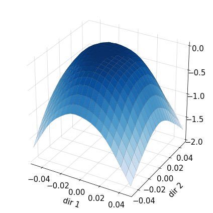
(a) Adv Training, $\epsilon=2$

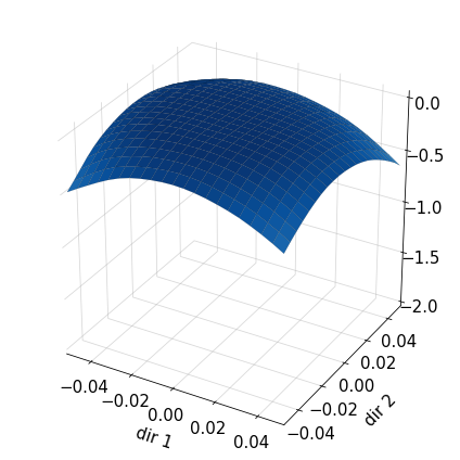
(b) Adv Training, $\epsilon=4$

(c) Adv Training, $\epsilon=6$

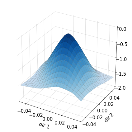
(d) Jacobian Reg, $\lambda=0.01$

(e) Jacobian Reg, $\lambda=0.05$

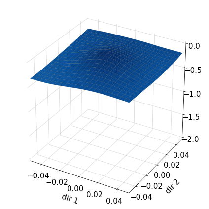
(f) Jacobian Reg, $\lambda=0.1$

Figure 2: Relative likelihood landscapes for Adversarial Training and Jacobian regularization with increasing strength. All models used DDNet trained on CIFAR10 and adversarial training uses PGD for 10 iterations. We see that stronger defenses tend to have have flatter landscapes.

We now describe how to utilize Eqn. 3 to visualize relative likelihood landscapes, building on top of prior work focusing on visualizing loss-landscapes [11, 22, 47]. To make these plots, we visualize the relative likelihood with respect to a clean sample in a surrounding neighborhood. Namely, for each point $x^{\prime}$ in the neighborhood $\mathtt{N}(x)$ surrounding a clean sample $x$, we plot $\Delta\log p_{\theta}(x^{\prime})$.

Consistent with prior work, we define the neighborhood $\mathtt{N}(x)$ around a clean sample as

$$\mathtt{N}(x)=\{x^{\prime}|x^{\prime}=x+\epsilon_{1}d+\epsilon_{2}d^{\perp}\}$$ (4)

where $d$ and $d^{\perp}$ are the two randomly pre-selected orthogonal signed vectors, and $\epsilon_{1}$ and $\epsilon_{2}$ represent the perturbation intensity along the axes $d$ and $d^{\perp}$. Visualizing $\Delta\log p(x^{\prime})$ for samples $x^{\prime}$ surrounding the clean sample $x$ allows us to understand the degree to which structured perturbations affect the likelihood of the sample under the model.

Fig. 1 shows such visualizations on a typical test-time example for standard training (no defense), adversarial training, and training with Jacobian regularization. Note that while we show just one example in these figures, we observe the same general trends over many samples. More examples of these plots can be found in the Appendix. Then as shown in Fig. 1a, for standard training small perturbations from the center clean image drops the likelihood of that sample considerably. While likelihood doesn’t necessarily correlate one to one with accuracy, it’s incredibly worrying that standard training doesn’t model data samples that are slightly perturbed from test examples. Furthermore, these images are test examples that the model hasn’t seen during training. This points to an underlying dataset bias, since the model has high likelihood for exactly the test example, but not for samples a small pixel perturbation away. This supports the recent idea that adversarial examples might be more of a property of datasets rather than the model themselves [17].

The rest of Fig. 1 shows that adversarial defenses like adversarial training and Jacobian regularization tend to have a much more uniform likelihood distribution, where perturbed points have a similar likelihood to the clean sample (i.e., the likelihood landscape is “flat”). Moreover, we also observe in Fig. 2 that the stronger the defense (for both adversarial training and Jacobian regularization), the lower the variation in the resulting relative likelihood landscape. Specifically, if we increase the adversarial training attack strength ($\epsilon$) or increase the Jacobian regularization strength ($\lambda$), we observe a “flatter” likelihood landscape. We measure this correlation quantitatively in Sec. 3.3.

To get an understanding of the impact different defenses have on the likelihood of overall data distribution, we further plot the histogram of $\log p_{\theta}(x)$ for all clean test samples and randomly perturbed samples near them (Fig. 3). Adversarial training and Jacobian regularization share several common effects on the log-likelihood distribution: (1) both techniques induce more aligned distribution between clean samples and randomly perturbed samples (likely as a consequence of likelihood landscape flattening). (2) both techniques tend to decrease the log-likelihood of clean samples relatively to randomly perturbed samples. (3) The stronger the regularization, the more left-skewed the log-likelihood distribution of clean samples is.

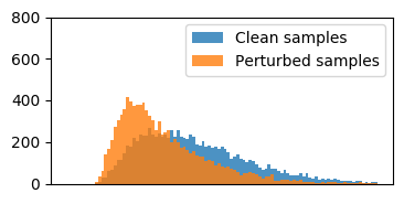
(a) Standard Training

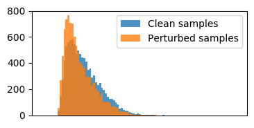
(b) Jacobian Reg, $\lambda=0.01$

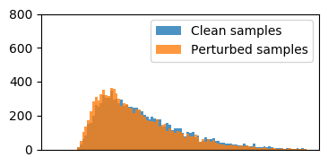
(c) Adversarial Training (AT), $\epsilon=2$

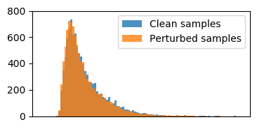
(d) Adversarial Training (AT), $\epsilon=5$

Figure 3: Histograms of log-likelihood $\log p_{\theta}(x)$ for clean samples and randomly perturbed samples. Blue corresponds to the log-likelihood on clean samples in CIFAR10 while orange corresponds to the log-likelihood on the perturbed samples. Note that the x-axis for plots might be differently shifted due to the different unknown normalizing constant $Z(\theta)$ for each model, but the scale of x-axis are the same across plots. (a) visualizes DDNet trained without additional defense, (b) uses a Jacobian regularized DDNet and (c)(d) use DDNet trained using PGD based adversarial training for 10 iterations. We see in adversarially robust approaches, clean and perturbed samples have more aligned distributions. We also note that with stronger regularization the distributions become increasingly left-skewed.

3.3 Quantifying Flatness

To quantify the degree of variation in the likelihood landscape surrounding a point, we use the Approximate Mass Score (AMS), which was originally introduced in [12] as an out of distribution detection score. AMS depends on how the marginal likelihood changes in the immediate neighborhood of a point in the input space. The Approximate Mass Score can be expressed as,

$$s_{\theta}(x)=-\left|\left|\frac{\partial\log p_{\theta}(x)}{\partial x}\right|\right|_{F}$$ (5)

We use the gradient for all $x^{\prime}\in\mathtt{N}(x)$ as an indicator of the “flatness” of the likelihood landscape surrounding the clean sample. While $\log p_{\theta}(x)$ is intractable to compute in practice, we can compute $\frac{\partial\log p_{\theta}(x)}{\partial x}$ exactly,

$$\frac{\partial\log p_{\theta}(x)}{\partial x} =\frac{\partial}{\partial x}\log\left(\frac{\sum_{y}\exp{(f_{\theta,y}(x)})}{Z(\theta)}\right)=\sum_{y}p_{\theta}(y|x)\frac{\partial f_{\theta,y}(x)}{\partial x}$$ (6)

To quantify the flatness in the surrounding area of $x$, we sample this quantity at each point in the neighborhood of $x$ (see Eq. 4) and average over $n$ random choices for $d$ and $d^{\perp}$ to obtain:

$$\phi(x)=\sum_{j=1}^{n}\sum_{x^{\prime}\in\mathtt{N}_{j}(x)}\frac{s_{\theta}(x)}{n}=\sum_{j=1}^{n}\sum_{x^{\prime}\in\mathtt{N}_{j}(x)}\frac{-1}{n}\left|\left|\frac{\partial\log p_{\theta}(x^{\prime})}{\partial x}\right|\right|_{F}$$ (7)

The flatness of likelihood landscape for a model is then calculated by averaging $\phi(x)$ for all testing samples.

$$\Phi=\sum_{i=1}^{N}\frac{\phi(x_{i})}{N}$$ (8)

Fig. 4 shows the relationship between flatness score $\Phi$ and defense strength. For both adversarial training (Fig. 4a) and Jacobian regularization (Fig. 4b), the stronger the defense, the lower the score and the higher the adversarial accuracy. This observation motivates us to explore directly regularizing this AMS term (AMSReg) to induce a flat likelihood landscape.

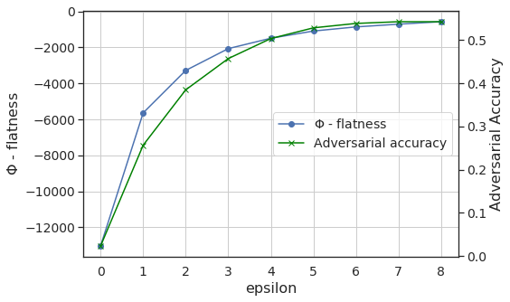
(a) Adversarial training

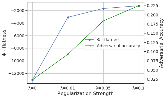
(b) Jacobian regularization

Figure 4: Visualizes the relationship between the likelihood landscape flatness (as defined by Eqn. 8) and adversarial accuracy. (a) showcases DDNet trained on CIFAR10 using PGD based adversarial training for 10 iterations with increasing epsilon strength. (b) showcases DDNet trained on CIFAR10 using Jacobian regularization of increasing strength. We see that adversarial accuracy and flatness of the relative likelihood landscape are correlated in the case of both defenses.

3.4 Approximate Mass Score Regularization (AMSReg)

In our experiments, we observe that high adversarial robustness corresponds with a low Approximate Mass Score in the case of both adversarial training and Jacobian regularization. This begs the question, is it possible to improve adversarial robustness by directly regularizing this term? That is, can we regularize $\left|\left|\frac{\partial\log p_{\theta}(x)}{\partial x}\right|\right|_{F}^{2}$ directly in addition to the cross-entropy loss to encourage robust predictive performance? Note however that naively computing this term during training would require double backpropagation, which would be inefficient.

Instead we make the observation that the right hand side of Eqn. 6 (used to compute $\frac{\partial\log p_{\theta}(x)}{\partial x}$) is reminiscent of gradient regularization techniques – specifically, Jacobian Regularization [16].

Connection with Jacobian Regularization [16]. As discussed in [16], Jacobian regularization traditionally emerges as a consequence of stability analysis of model predictions against input perturbations – the high-level idea being that small input perturbations should minimally affect the predictions made by a network up to a first order Taylor expansion. Hoffman et al. [16] characterize this by regularizing the Jacobian of the output logits with respect to the input images. The difference between each element being summed over in the right hand side of Eqn. 6 and the input-output Jacobian term used in [16] is that now the Jacobian term is weighted by the predicted probability of each class. Namely, optimizing $\left|\left|\frac{\partial\log p_{\theta}(x)}{\partial x}\right|\right|_{F}^{2}$ results in regularizing $||\sum_{c}p_{\theta}(c\mid x)\frac{\partial f_{\theta,c}(x)}{\partial x}||_{F}^{2}$, while Jacobian regularization regularizes just $||\frac{\partial f_{\theta,c}(x)}{\partial x}||_{F}^{2}$. The following proposition provides an upper bound of the squared norm that can be efficiently calculated in batch when using the efficient algorithm proposed for Jacobian regularization in [16].

Proposition 3.1. Let $C$ denote the number of classes, and $J^{w}(x)=p_{\theta}(c\mid x)\frac{\partial f_{\theta,c}(x)}{\partial x_{i}}$ be a weighted variant of the Jacobian of the class logits with respect to the input. Then, the frobenius norm of $J^{w}(x)$ multiplied by the total number of classes upper bounds the AMS score:

$$\left|\left|\frac{\partial\log p_{\theta}(x)}{\partial x}\right|\right|_{F}^{2}\leq C\left|\left|J^{w}(x)\right|\right|_{F}^{2}$$ (9)

Proof. Recall that as per the EBM [12] interpretation of a discriminative classifier, $\frac{\partial\log p_{\theta}(x)}{\partial x}$ can be expressed as,

$$\frac{\partial\log p_{\theta}(x)}{\partial x} =\frac{\partial}{\partial x}\log\left(\frac{\sum_{y}\exp{(f_{\theta,y}(x)})}{Z(\theta)}\right)$$ (10)

$$=\frac{\partial}{\partial x}\log\sum\nolimits_{y}\exp(f_{\theta,y}(x))$$ (11)

$$=\sum\nolimits_{y}\frac{\exp(f_{\theta,y}(x))}{\sum\nolimits_{y}\exp(f_{\theta,y}(x))}\frac{\partial f_{\theta,y}(x)}{\partial x}$$ (12)

Or,

$$\frac{\partial\log p_{\theta}(x)}{\partial x}=\sum\nolimits_{y}p_{\theta}(y\mid x)\frac{\partial f_{\theta,y}(x)}{\partial x}$$ (14)

We utilize the Cauchy-Schwarz inequality, as stated below to obtain an upper bound on $\frac{\partial\log p_{\theta}(x)}{\partial x}$

$$(\sum_{k=1}^{N}u_{k}v_{k})^{2}\leq(\sum_{k=1}^{N}u_{k}^{2})(\sum_{k=1}^{N}v_{k}^{2})$$ (15)

where $u_{k},v_{k}\in\mathbb{R}\text{ for all }k\in\{1,2,...,N\}$. If we set $u_{k}=1$ for all $k$, the inequality reduces to,

$$(\sum_{k=1}^{N}v_{k})^{2}\leq N(\sum_{k=1}^{N}v_{k}^{2})$$ (16)

Since, $J^{w}_{y,i}(x)\in\mathbb{R}$, we have,

$$(\sum_{y=1}^{C}J^{w}_{y,i}(x))^{2}\leq C\sum_{y=1}^{C}(J^{w}_{y,i}(x))^{2}$$ (17)

where $C$ is the total number of output classes. This implies that,

$$\sum_{i}(\sum_{y=1}^{C}J^{w}_{y,i}(x))^{2}\leq C\sum_{i}\sum_{y=1}^{C}(J^{w}_{y,i}(x))^{2}$$ (18)

Or,

$$\left|\left|\frac{\partial\log p_{\theta}(x)}{\partial x}\right|\right|_{F}^{2}\leq C\left|\left|J^{w}(x)\right|\right|_{F}^{2}$$ (19)

To summarize, the overall objective we optimize for a mini-batch $B=\{(x,y)\}_{i=1}^{|B|}$ using AMSReg can be expressed as,

$$\mathcal{L}_{\text{Joint}}(B;\theta)=\sum_{(x,y)\in B}\mathcal{L}_{\text{CE}}(x,y;\theta)+\frac{\mu}{2}\left[\frac{1}{|B|}\sum_{x\in B}\left|\left|J^{w}(x)\right|\right|_{F}^{2}\right]$$ (20)

where $\mathcal{L}_{\text{CE}}(x,y;\theta)$ is the standard cross-entropy loss function and $\mu$ is a hyperparameter that determines the strength of regularization.

Efficient Algorithm for AMSReg. Hoffman et al., [16] introduce an efficient algorithm to calculate the Frobenius norm of the input-output Jacobian ($J_{y,i}(x)=\frac{\partial f_{\theta,y}(x)}{\partial x_{i}}$) using random projection as,

$$||J{(x)}||_{F}^{2}=C\mathbb{E}_{\hat{v}\sim S^{C-1}}[||\hat{v}\cdot J||^{2}]$$ (21)

where $C$ is the total number of output classes and $\hat{v}$ is random vector drawn from the $(C-1)$-dimensional unit sphere $S^{C-1}$. $||J{(x)}||_{F}^{2}$ can then be efficiently approximated by sampling random vectors as,

$$||J{(x)}||_{F}^{2}\approx\frac{1}{n_{proj}}\sum^{n_{proj}}_{\mu=1}[\frac{\partial(\hat{v}^{\mu}\cdot z)}{\partial x}]^{2}$$ (22)

where $n_{proj}$ is the number of random vectors drawn and $z$ is the output vector (see Section 2.3 [16] for more details). In AMSReg, we optimize the square of the Frobenius norm of $J^{w}(x)$ where:

$$J^{w}_{y,i}(x)=p_{\theta}(y\mid x)\frac{\partial f_{\theta,y}(x)}{\partial x_{i}}$$ (23)

Since $J^{w}{(x)}$ can essentially be expressed as a matrix product of a diagonal matrix of predicted class probabilities and the regular Jacobian matrix, we are able to re-use the efficient random projection algorithm by expressing $||J^{w}{(x)}||_{F}^{2}$ as,

$$||J^{w}{(x)}||_{F}^{2}=C\mathbb{E}_{\hat{v}\sim S^{C-1}}[||\hat{v}^{T}\mathtt{diag}(p_{\theta}(c\mid x))J(x)||^{2}]$$ (24)

3.5 Experiments with AMSReg

We run our experiments on the CIFAR-10 and Fashion-MNIST datasets [45]. We compare AMSReg against both Adversarial Training (AT) [24] and Jacobian Regularization (Jacobian Reg.) [16]. We perform our experiments across three network architectures – LeNet [20], DDNet [30] and ResNet18 [15]. We train each model for 200 epochs using piecewise learning rate decay (i.e. decay ten-fold after the 100th and 150th epoch). All models are optimized using SGD with a momentum factor of 0.9. Adversarial training models are trained with 10 steps of PGD. When evaluating adversarial robustness, we use an $l_{\infty}$ bounded 5-steps PGD attack with $\epsilon=8/255$ and a step size of $2/255$ for models trained on CIFAR10 and a 10-step PGD attack with $\epsilon=25/255$ and a step size of $6.25/255$ for models trained on Fashion-MNIST.

Table 1: Experiments on CIFAR10: flatness $\Phi$ and accuracies(%) on clean and adversarial test samples. PGD attacks are generated with $\epsilon=8/255$, steps=5 and a step size of 2/255. AMSReg is able to achieve the highest $\Phi$-Flatness while adversarial training is the most robust defense.

		Defense		$\Phi$ (Flatness $\uparrow$)	Clean-Acc. $\uparrow$ (%)	Adversarial-Acc. $\uparrow$ (%) (PGD)
DDNet [30]		No Defense		$-13035.5$	$\mathbf{91.45}$	$1.7$
		AT ($\epsilon=3/255$)		$-2066.4$	$85.90$	$\mathbf{45.71}$
		Jacobian Reg. [16] ($\lambda=0.05$)		$-1692.6$	$86.06$	$18.31$
		AMSReg ($\lambda=1.0$)		$\mathbf{-768.7}$	$85.45$	$20.78$
RN-18 [15]		No Defense		$-13974.3$	$\mathbf{94.69}$	$0.1$
		AT ($\epsilon=3/255$)		$-1055.0$	$85.32$	$\mathbf{57.48}$
		Jacobian Reg. [16] ($\lambda=0.05$)		$-1945.1$	$82.28$	$14.73$
		AMSReg ($\lambda=1.0$)		$\mathbf{-659.5}$	$86.94$	$11.07$

Results and Analysis. Table 1 and Table 2 show the results of AMSReg compared to adversarial training and Jacobian regularization on CIFAR10 and Fashion-MNIST. It is known that there is a trade-off between adversarial robustness and accuracy [49, 41]. Therefore, here we only compare models that have similar accuracy on clean test images. As observed in Table 1 and 2, models trained with AMSReg indeed have flatter likelihood landscapes than Jacobian regularization and adversarial training, indicating that the regularization was successful. Furthermore, AMSReg models have comparable adversarial robustness to that of Jacobian regularization. However, they are still significantly susceptible to adversarial attacks than adversarial training.

Table 2: Experiments on Fashion-MNIST: flatness $\Phi$ and accuracies(%) on clean and adversarial test samples. PGD attacks are generated with $\epsilon=25/255$, steps=10 and a step size of 6.25/255. AMSReg is able to achieve the highest $\Phi$-Flatness while adversarial training is the most robust defense.

		Defense		$\Phi$ (Flatness $\uparrow$)	Clean-Acc. $\uparrow$ (%)	Adversarial-Acc. $\uparrow$ (%) (PGD)
LeNet [20]		No Defense		$-9435.9$	$\mathbf{91.53}$	$0.0$
		AT ($\epsilon=10/255$)		$-1504.0$	$89.35$	$\mathbf{62.64}$
		Jacobian Reg. [16] ($\lambda=0.01$)		$-1694.6$	$88.76$	$34.71$
		AMSReg ($\lambda=0.5$)		$\mathbf{-378.1}$	$89.51$	$34.04$
RN-18 [15]		No Defense		$-12952.8$	$\mathbf{93.75}$	$0.1$
		AT ($\epsilon=10/255$)		$-1257.8$	$91.64$	$\mathbf{65.24}$
		Jacobian Reg. [16] ($\lambda=0.01$)		$-821.7$	$91.04$	$45.37$
		AMSReg ($\lambda=0.5$)		$\mathbf{-482.9}$	$91.29$	$46.06$

We conduct further analysis by looking at the flatness along the attack directions (i.e., the direction an FGSM attack chosen to perturb the image) instead of random directions. Fig. 5 shows the likelihood landscape projected using one FGSM direction and one random direction. Interestingly enough, both Jacobian and AMS regularization are able to flatten the landscape in the random direction well (with AMS being slightly flatter than Jacobian). However, neither regularization method is able to flatten out the FGSM attack direction nearly as much as adversarial training. This might explain why neither AMS nor Jacobian regularization are able to match the adversarial robustness of adversarial training. We leave the next step of flattening out the worst-case directions (i.e. the attack directions) for future work.

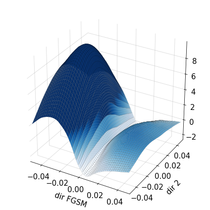
(a) Standard training

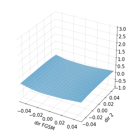
(b) Adv Train, $\epsilon=6$

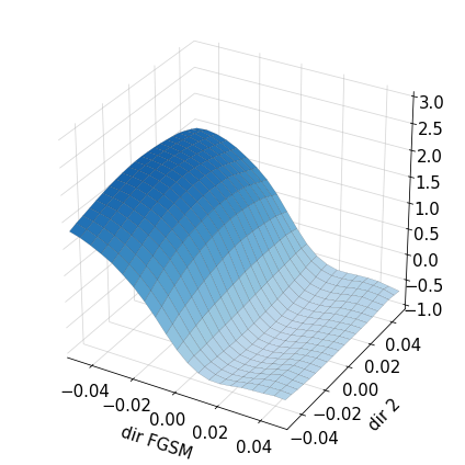
(c) AMSReg, $\lambda=1$

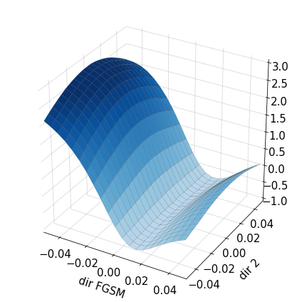
(d) Jacobian, $\lambda=0.1$

Figure 5: Relative likelihood landscapes projected using one FGSM direction (dir FGSM) and a random direction (dir2). Each visualization uses DDNet trained on CIFAR10. (a) uses standard training with no defense, (b) is adversarially trained with a 10-step PGD attack, (c) uses AMSReg with $\lambda=1$, and (d) uses Jacobian Regularization with $\lambda=0.1$. We see that adversarial training is able to flatten the likelihood landscape in the FGSM direction much more than the regularization defenses.

4 Conclusion

In this work, we explore why neural networks are vulnerable to adversarial attacks from a perspective of the marginal distribution of the inputs (images) under the trained model. We first suggest a way to visualize the likelihood landscape of CNNs by leveraging the recently proposed EBM interpretation of a discriminatively learned classifier. Qualitatively, we show that a subset of standard defense techniques such as adversarial training and Jacobian regularization share a common pattern: they induce flat likelihood landscapes. We then quantitatively show this correlation by introducing a measure regarding the flatness of the likelihood landscape in the surrounding area of clean samples. We also explore directly regularizing a term that encourages flat likelihood landscapes, but this results in worse adversarial robustness than adversarial training and is roughly comparable to just Jacobian regularization. After further analysis, we find that adversarial training significantly flattens the likelihood landscape in the directions abused by adversarial attacks. The regularization methods, on the other hand, are better at flattening the landscape in random directions. These findings suggest that flattening the likelihood landscape is important for adversarial robustness, but it’s most important for the landscape to be flat in the directions chosen by adversarial attacks.

Overall, our findings in this paper provide a new perspective of adversarial robustness as flattening the likelihood landscape and show how different defenses and regularization techniques address this similar core deficiency. We leave designing a regularizer that flattens the likelihood landscape in attack directions for future investigation.

Appendix 0.A Appendix

In this section, we first provide some details on the efficient algorithm used to compute AMSReg (see Section 3.4, main paper) during training. Next, we present some additional examples of our relative likelihood landscape visualization.

0.A.1 Details on the efficient algorithm implementation for AMSReg.

Hoffman et al., [16] introduce an efficient algorithm to calculate the Frobenius norm of the input-output Jacobian ($J_{y,i}(x)=\frac{\partial f_{\theta,y}(x)}{\partial x_{i}}$) using random projection as,

$$||J{(x)}||_{F}^{2}=C\mathbb{E}_{\hat{v}\sim S^{C-1}}[||\hat{v}\cdot J||^{2}]$$ (25)

where $C$ is the total number of output classes and $\hat{v}$ is random vector drawn from the $(C-1)$-dimensional unit sphere $S^{C-1}$. $||J{(x)}||_{F}^{2}$ can then be efficiently approximated by sampling random vectors as,

$$||J{(x)}||_{F}^{2}\approx\frac{1}{n_{proj}}\sum^{n_{proj}}_{\mu=1}[\frac{\partial(\hat{v}^{\mu}\cdot z)}{\partial x}]^{2}$$ (26)

where $n_{proj}$ is the number of random vectors drawn and $z$ is the output vector (see Section 2.3 [16] for more details). In AMSReg, we optimize the square of the Frobenius norm of $J^{w}(x)$ where:

$$J^{w}_{y,i}(x)=p_{\theta}(y\mid x)\frac{\partial f_{\theta,y}(x)}{\partial x_{i}}$$ (27)

Since $J^{w}{(x)}$ can essentially be expressed as a matrix product of a diagonal matrix of predicted class probabilities and the regular Jacobian matrix, we are able to re-use the efficient random projection algorithm by expressing $||J^{w}{(x)}||_{F}^{2}$ as,

$$||J^{w}{(x)}||_{F}^{2}=C\mathbb{E}_{\hat{v}\sim S^{C-1}}[||\hat{v}^{T}\mathtt{diag}(p_{\theta}(c\mid x))J(x)||^{2}]$$ (28)

0.A.2 More examples of likelihood landscape visualization

We show more examples of relative likelihood landscape visualization that are similar to Fig. 2 in the main paper but are for different test samples and network architectures. Concretely, Fig. 6 and Fig. 7 shows the relative likelihood landscapes for two test samples of CIFAR10 using DDNet [30] model trained with different defenses. Fig. 8 shows the relative likelihood landscapes for one test sample of CIFAR10 using ResNet18 [15] model trained with different defenses. Overall, we can see that stronger defenses tend to have flatter landscapes.

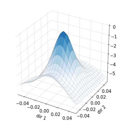
(a) Standard training

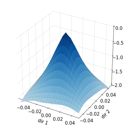
(b) Jacobian Reg, $\lambda=0.01$

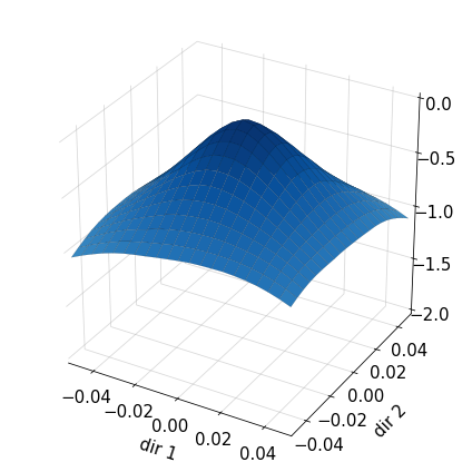
(c) Jacobian Reg, $\lambda=0.1$

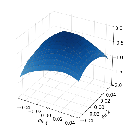
(d) Adv Training, $\epsilon=2$

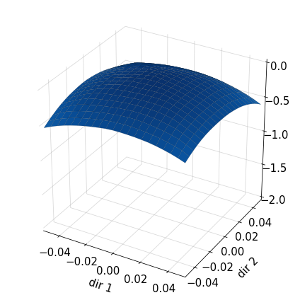
(e) Adv Training, $\epsilon=4$

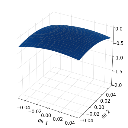
(f) Adv Training, $\epsilon=8$

Figure 6: Relative likelihood landscapes for Adversarial Training and Jacobian regularization with increasing strength. All models used DDNet trained on CIFAR10 and adversarial training uses PGD for 10 iterations.

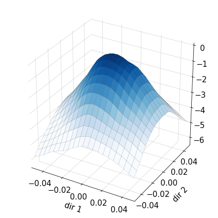
(a) Standard training

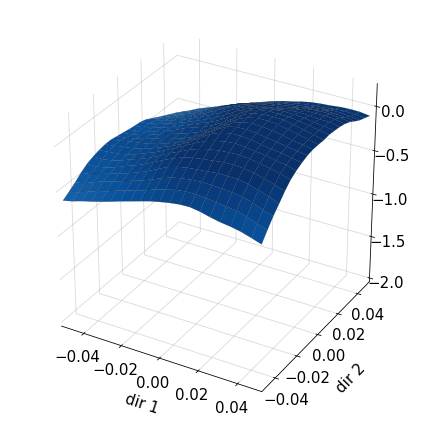
(b) Jacobian Reg, $\lambda=0.01$

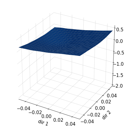
(c) Jacobian Reg, $\lambda=0.1$

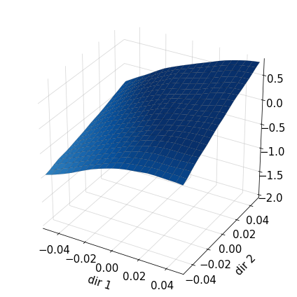
(d) Adv Training, $\epsilon=2$

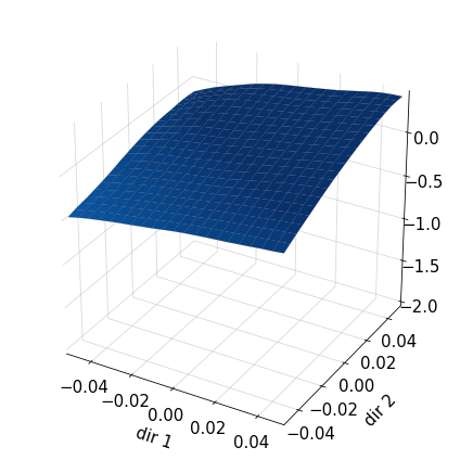
(e) Adv Training, $\epsilon=4$

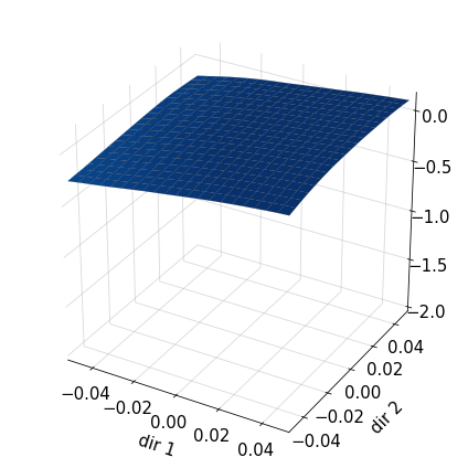
(f) Adv Training, $\epsilon=8$

Figure 7: Relative likelihood landscapes for Adversarial Training and Jacobian regularization with increasing strength. All models used DDNet trained on CIFAR10 and adversarial training uses PGD for 10 iterations.

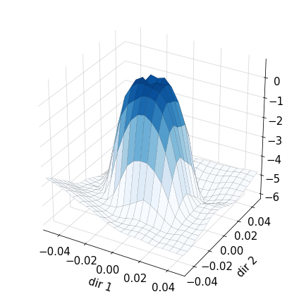
(a) Standard training

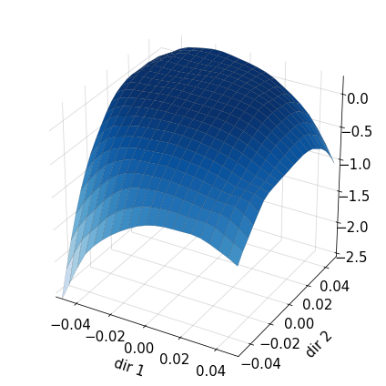
(b) Adv Training, $\epsilon=1$

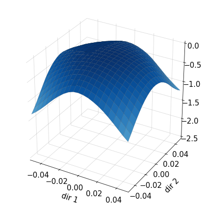
(c) Adv Training, $\epsilon=3$

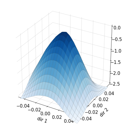
(d) Jacobian Reg, $\lambda=0.01$

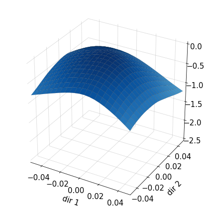
(e) Jacobian Reg, $\lambda=0.05$

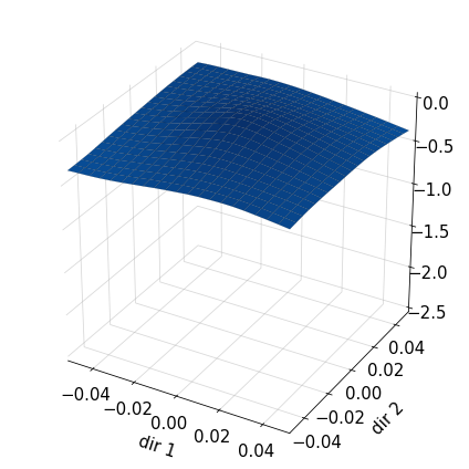
(f) Jacobian Reg, $\lambda=0.1$

Figure 8: Relative likelihood landscapes for Adversarial Training and Jacobian regularization with increasing strength. All models used ResNet18 trained on CIFAR10 and adversarial training uses PGD for 10 iterations.

References

- [1] Antol, S., Agrawal, A., Lu, J., Mitchell, M., Batra, D., Lawrence Zitnick, C., Parikh, D.: VQA: Visual Question Answering. In: Intl. Conf. on Computer Vision (2015)
- [2] Carlini, N., Wagner, D.: Towards evaluating the robustness of neural networks. In: 2017 ieee symposium on security and privacy (sp). pp. 39–57. IEEE (2017)
- [3] Das, A., Kottur, S., Gupta, K., Singh, A., Yadav, D., Moura, J.M., Parikh, D., Batra, D.: Visual Dialog. In: Proceedings of the IEEE Conference on Computer Vision and Pattern Recognition (CVPR) (2017)
- [4] Doersch, C., Gupta, A., Efros, A.A.: Unsupervised visual representation learning by context prediction. In: Proceedings of the IEEE international conference on computer vision. pp. 1422–1430 (2015)
- [5] Drucker, H., Le Cun, Y.: Improving generalization performance using double backpropagation. IEEE Transactions on Neural Networks 3(6), 991–997 (1992)
- [6] Engstrom, L., Ilyas, A., Santurkar, S., Tsipras, D., Tran, B., Madry, A.: Adversarial robustness as a prior for learned representations. arXiv preprint arXiv:1906.00945 (2019)
- [7] Feinman, R., Curtin, R.R., Shintre, S., Gardner, A.B.: Detecting adversarial samples from artifacts. arXiv preprint arXiv:1703.00410 (2017)
- [8] Girshick, R.: Fast r-cnn. In: Proceedings of the IEEE International Conference on Computer Vision. pp. 1440–1448 (2015)
- [9] Goodfellow, I., Pouget-Abadie, J., Mirza, M., Xu, B., Warde-Farley, D., Ozair, S., Courville, A., Bengio, Y.: Generative adversarial nets. In: Advances in neural information processing systems. pp. 2672–2680 (2014)
- [10] Goodfellow, I.J., Shlens, J., Szegedy, C.: Explaining and harnessing adversarial examples. arXiv preprint arXiv:1412.6572 (2014)
- [11] Goodfellow, I.J., Vinyals, O., Saxe, A.M.: Qualitatively characterizing neural network optimization problems. arXiv preprint arXiv:1412.6544 (2014)
- [12] Grathwohl, W., Wang, K.C., Jacobsen, J.H., Duvenaud, D., Norouzi, M., Swersky, K.: Your classifier is secretly an energy based model and you should treat it like one. arXiv preprint arXiv:1912.03263 (2019)
- [13] Gu, S., Rigazio, L.: Towards deep neural network architectures robust to adversarial examples. arXiv preprint arXiv:1412.5068 (2014)
- [14] Guo, C., Rana, M., Cisse, M., Van Der Maaten, L.: Countering adversarial images using input transformations. arXiv preprint arXiv:1711.00117 (2017)
- [15] He, K., Zhang, X., Ren, S., Sun, J.: Deep residual learning for image recognition. In: Proceedings of the IEEE conference on computer vision and pattern recognition. pp. 770–778 (2016)
- [16] Hoffman, J., Roberts, D.A., Yaida, S.: Robust learning with jacobian regularization. arXiv preprint arXiv:1908.02729 (2019)
- [17] Ilyas, A., Santurkar, S., Tsipras, D., Engstrom, L., Tran, B., Madry, A.: Adversarial examples are not bugs, they are features. In: Advances in Neural Information Processing Systems. pp. 125–136 (2019)
- [18] Jakubovitz, D., Giryes, R.: Improving dnn robustness to adversarial attacks using jacobian regularization. In: Proceedings of the European Conference on Computer Vision (ECCV). pp. 514–529 (2018)
- [19] Kurakin, A., Goodfellow, I., Bengio, S.: Adversarial examples in the physical world. arXiv preprint arXiv:1607.02533 (2016)
- [20] Lecun, Y., Bottou, L., Bengio, Y., Haffner, P.: Gradient-based learning applied to document recognition. Proceedings of the IEEE 86(11), 2278–2324 (Nov 1998). https://doi.org/10.1109/5.726791
- [21] Lee, K., Lee, K., Lee, H., Shin, J.: A simple unified framework for detecting out-of-distribution samples and adversarial attacks. In: Advances in Neural Information Processing Systems. pp. 7167–7177 (2018)
- [22] Li, H., Xu, Z., Taylor, G., Studer, C., Goldstein, T.: Visualizing the loss landscape of neural nets. In: Advances in Neural Information Processing Systems. pp. 6389–6399 (2018)
- [23] Ma, X., Li, B., Wang, Y., Erfani, S.M., Wijewickrema, S., Schoenebeck, G., Song, D., Houle, M.E., Bailey, J.: Characterizing adversarial subspaces using local intrinsic dimensionality. arXiv preprint arXiv:1801.02613 (2018)
- [24] Madry, A., Makelov, A., Schmidt, L., Tsipras, D., Vladu, A.: Towards deep learning models resistant to adversarial attacks. arXiv preprint arXiv:1706.06083 (2017)
- [25] Moosavi-Dezfooli, S.M., Fawzi, A., Uesato, J., Frossard, P.: Robustness via curvature regularization, and vice versa. In: Proceedings of the IEEE Conference on Computer Vision and Pattern Recognition. pp. 9078–9086 (2019)
- [26] Pang, T., Du, C., Dong, Y., Zhu, J.: Towards robust detection of adversarial examples. In: Advances in Neural Information Processing Systems. pp. 4579–4589 (2018)
- [27] Pang, T., Xu, K., Dong, Y., Du, C., Chen, N., Zhu, J.: Rethinking softmax cross-entropy loss for adversarial robustness. arXiv preprint arXiv:1905.10626 (2019)
- [28] Pang, T., Xu, K., Zhu, J.: Mixup inference: Better exploiting mixup to defend adversarial attacks. arXiv preprint arXiv:1909.11515 (2019)
- [29] Papernot, N., McDaniel, P., Jha, S., Fredrikson, M., Celik, Z.B., Swami, A.: The limitations of deep learning in adversarial settings. In: 2016 IEEE European symposium on security and privacy (EuroS&P). pp. 372–387. IEEE (2016)
- [30] Papernot, N., McDaniel, P., Wu, X., Jha, S., Swami, A.: Distillation as a defense to adversarial perturbations against deep neural networks. In: 2016 IEEE Symposium on Security and Privacy (SP). pp. 582–597. IEEE (2016)
- [31] Qin, C., Martens, J., Gowal, S., Krishnan, D., Dvijotham, K., Fawzi, A., De, S., Stanforth, R., Kohli, P.: Adversarial robustness through local linearization. In: Advances in Neural Information Processing Systems. pp. 13824–13833 (2019)
- [32] Qin, Y., Frosst, N., Sabour, S., Raffel, C., Cottrell, G., Hinton, G.: Detecting and diagnosing adversarial images with class-conditional capsule reconstructions. arXiv preprint arXiv:1907.02957 (2019)
- [33] Raff, E., Sylvester, J., Forsyth, S., McLean, M.: Barrage of random transforms for adversarially robust defense. In: Proceedings of the IEEE Conference on Computer Vision and Pattern Recognition. pp. 6528–6537 (2019)
- [34] Ross, A.S., Doshi-Velez, F.: Improving the adversarial robustness and interpretability of deep neural networks by regularizing their input gradients. In: Thirty-second AAAI conference on artificial intelligence (2018)
- [35] Samangouei, P., Kabkab, M., Chellappa, R.: Defense-gan: Protecting classifiers against adversarial attacks using generative models. arXiv preprint arXiv:1805.06605 (2018)
- [36] Shafahi, A., Najibi, M., Ghiasi, M.A., Xu, Z., Dickerson, J., Studer, C., Davis, L.S., Taylor, G., Goldstein, T.: Adversarial training for free! In: Advances in Neural Information Processing Systems. pp. 3353–3364 (2019)
- [37] Sokolić, J., Giryes, R., Sapiro, G., Rodrigues, M.R.: Robust large margin deep neural networks. IEEE Transactions on Signal Processing 65(16), 4265–4280 (2017)
- [38] Svoboda, P., Hradis, M., Barina, D., Zemcik, P.: Compression artifacts removal using convolutional neural networks. arXiv preprint arXiv:1605.00366 (2016)
- [39] Szegedy, C., Zaremba, W., Sutskever, I., Bruna, J., Erhan, D., Goodfellow, I., Fergus, R.: Intriguing properties of neural networks. In: International Conference on Learning Representations (2014), http://arxiv.org/abs/1312.6199
- [40] Tramèr, F., Boneh, D.: Adversarial training and robustness for multiple perturbations. In: Advances in Neural Information Processing Systems. pp. 5866–5876 (2019)
- [41] Tsipras, D., Santurkar, S., Engstrom, L., Turner, A., Madry, A.: Robustness may be at odds with accuracy. arXiv preprint arXiv:1805.12152 (2018)
- [42] Varga, D., Csiszárik, A., Zombori, Z.: Gradient regularization improves accuracy of discriminative models. arXiv preprint arXiv:1712.09936 (2017)
- [43] Wan, W., Zhong, Y., Li, T., Chen, J.: Rethinking feature distribution for loss functions in image classification. In: Proceedings of the IEEE Conference on Computer Vision and Pattern Recognition. pp. 9117–9126 (2018)
- [44] Wong, E., Rice, L., Kolter, J.Z.: Fast is better than free: Revisiting adversarial training. arXiv preprint arXiv:2001.03994 (2020)
- [45] Xiao, H., Rasul, K., Vollgraf, R.: Fashion-mnist: a novel image dataset for benchmarking machine learning algorithms. arXiv preprint arXiv:1708.07747 (2017)
- [46] Xie, C., Wang, J., Zhang, Z., Ren, Z., Yuille, A.: Mitigating adversarial effects through randomization. arXiv preprint arXiv:1711.01991 (2017)
- [47] Yu, F., Qin, Z., Liu, C., Zhao, L., Wang, Y., Chen, X.: Interpreting and evaluating neural network robustness. arXiv preprint arXiv:1905.04270 (2019)
- [48] Zhang, D., Zhang, T., Lu, Y., Zhu, Z., Dong, B.: You only propagate once: Accelerating adversarial training via maximal principle. In: Advances in Neural Information Processing Systems. pp. 227–238 (2019)
- [49] Zhang, H., Yu, Y., Jiao, J., Xing, E.P., Ghaoui, L.E., Jordan, M.I.: Theoretically principled trade-off between robustness and accuracy. arXiv preprint arXiv:1901.08573 (2019)
- [50] Zheng, Z., Hong, P.: Robust detection of adversarial attacks by modeling the intrinsic properties of deep neural networks. In: Advances in Neural Information Processing Systems. pp. 7913–7922 (2018)