Can a protophobic vector boson explain the ATOMKI anomaly?

Abstract

In 2016, the ATOMKI collaboration announced [PRL 116, 042501 (2016)] observing an unexpected enhancement of the $e^{+}$-$e^{-}$pair production signal in one of the ${}^{8}\mathrm{Be}$ nuclear transitions induced by an incident proton beam on a ⁷Li target. Many beyond-standard-model physics explanations have subsequently been proposed. One popular theory is that the anomaly is caused by the creation of a protophobic vector boson ($X$) with a mass around 17 MeV [e.g., PRL 117, 071803 (2016)] in the nuclear transition. We study this hypothesis by deriving an isospin relation between photon and $X$ couplings to nucleons. This allows us to find simple relations between protophobic $X$-production cross sections and those for measured photon production. The net result is that $X$ production is dominated by direct transitions induced by $E1^{X}$ and $L1^{X}$ (transverse and longitudinal electric dipoles) and $C1^{X}$ (charge dipole) without going through any nuclear resonance (i.e. Bremsstrahlung radiation) with a smooth energy dependence that occurs for all proton beam energies above threshold. This contradicts the experimental observations and invalidates the protophobic vector boson explanation.

Ref. Krasznahorkay:2015iga observed an anomaly in measuring $e^{+}$-$e^{-}$pair production in ${}^{8}\mathrm{Be}$’s nuclear transition between the 18.15 MeV $1^{+}$ resonance and its $0^{+}$ ground state. Fig. 1 shows the relevant energy levels Tilley:2004zz . The two $1^{+}$ resonances are barely above the ${}^{7}\mathrm{Li}+p$ threshold. The unexpected enhancement of the signal was observed in the large $e^{+}$-$e^{-}$invariant mass region (about 17 MeV) and in the large pair-correlation angles (near $140^{\circ}$) region. The large angle enhancement is a simple kinematic signature of the decay of a heavy particle into an $e^{+}-e^{-}$ pair. The anomaly has generated many beyond-standard-model physics explanations (e.g., Krasznahorkay:2015iga ; Feng:2016jff ; others ).

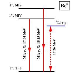
Figure 1: The ${}^{8}\mathrm{Be}$ levels Tilley:2004zz that are relevant for the M1 transitions producing photon ($\gamma$) and recently proposed vector boson $X$ Feng:2016jff ; Feng:2016ysn ; Feng:2020mbt . The two $1^{+}$ resonance states are either mostly isovector (MIV) or mostly isoscalar (MIS). The blue line is the ${}^{7}\mathrm{Li}+p$ threshold. Note $X$ and (off-shell) $\gamma$ can further decay into $e^{+}$-$e^{-}$.

Our focus is on the protophobic vector boson explanation (see e.g. Feng:2016jff ; Feng:2016ysn ; Feng:2020mbt ). We shall show that taking this hypothesis seriously leads to the result that the large angle enhancement of pair-production would have been seen at all ATOMKI energies above threshold.

The physics of a boson that almost does not interact with protons provides an interesting contrast with photon-nucleon interactions. We next show that isospin symmetry enables the derivation of a useful relation between the matrix elements of the two interactions.

The photon-quark interactions are given by the following electromagnetic (EM) current in its $2^{\mathrm{nd}}$ quantization form:

$$j^{\mu}_{\gamma} =\overline{Q}\gamma^{\mu}\left({1\over 6}+{\tau_{3}\over 2}\right)Q=j^{\mu}_{s}+j^{\mu}_{v}\ ,\ \mathrm{with}$$

$$j^{\mu}_{s} \equiv\overline{Q}\gamma^{\mu}{1\over 6}Q\ ,\ j^{\mu}_{v}\equiv\overline{Q}\gamma^{\mu}{\tau_{3}\over 2}Q\ .$$ (1)

Here, $Q\equiv(u\ ,d)^{T}$ is the iso-doublet quark field operator $\tau_{3}$ the isospin Pauli matrix, and $j^{\mu}_{v}$ and $j^{\mu}_{s}$ as the isovector and isoscalar components of $j^{\mu}_{\gamma}$.

The general form of the coupling between a new vector boson $(X)$ and quarks is expressed in terms of a different linear combination of $j^{\mu}_{s}$ and $j^{\mu}_{v}$ Feng:2016ysn ; Feng:2020mbt :

$$j^{\mu}_{X}=\overline{Q}\gamma^{\mu}\left({\varepsilon_{s}\over 6}-{\varepsilon_{v}\tau_{3}\over 2}\right)Q=\varepsilon_{s}j^{\mu}_{s}-\varepsilon_{v}j^{\mu}_{v},$$ (2)

where $\varepsilon_{s}$ and $(-\varepsilon_{v})$ are the ratios between the $X$ and $\gamma$ coupling constants in the isoscalar and isovector components. When $\varepsilon_{s}\approx\varepsilon_{v}$, $X$ is considered to be protophobic, because the $X$-proton charge-coupling would be much smaller than the $X$-neutron one. In fact, with $\varepsilon_{s}=\varepsilon_{v}$ the $X$-$p$ charge coupling vanishes because there are two $u$ and one $d$ valence quarks in proton, but $X$-$n$ charge coupling is $\varepsilon_{v}$ times that of $\gamma$-$p$.

Comparing Eq. (1) and Eq. (2) shows that apart from the factor $\varepsilon_{s}$ the isoscalar ($p+n$) current operators of the $\gamma$ and $X$ are the same, but (apart from the factor $\varepsilon_{v}$) the isovector ($p-n$) matrix current operators differ by a minus sign.

The connection between quark operators and nucleon matrix elements is made explicit using invariance under the isospin rotation $P_{cs}\equiv P_{y}(\pi)$ Miller:1990iz ; Miller:2006tv , a rotation along $y$-axis by $180^{\circ}$ in the isospin space, that interchanges $p$ and $n$ and also (because isospin is an additive quantum number) $d$ and $u$. Invariance under this rotation gives

$$\langle p|j_{s}^{\mu}|p\rangle=\langle n|j_{s}^{\mu}|n\rangle,\,\quad\langle p|j_{v}^{\mu}|p\rangle=-\langle n|j_{v}^{\mu}|n\rangle.$$ (3)

Hence the nucleon-level isoscalar $X$-boson current operator is obtained by multiplying the isoscalar photon operator by $\varepsilon_{s}$ and the nucleon-level isovector $X$-boson current operator is obtained by multiplying the isovector photon operator by $-\varepsilon_{v}$.

In obtaining Eq. (3) isospin symmetry is assumed to be exact. That isospin violation in the nucleon wave function is very small can be anticipated from the small ratio of the neutron-proton mass difference to their average mass of order $10^{-3}$, and is also verified by explicit calculations, see e.g. Miller:1997ya .)

Therefore, $j^{\mu}_{s}$ and $j^{\mu}_{v}$’s matrix elements between nucleons are related to the isoscalar and isovector parts of the EM current’s matrix elements (with $u$ as the relevant Dirac spinor ):

$$\langle p|j_{s}^{\mu}|p\rangle=\frac{1}{2}\left(\langle p|j_{\gamma}^{\mu}|p\rangle+\langle n|j_{\gamma}^{\mu}|n\rangle\right)\equiv\overline{u}\,\Gamma^{\mu}_{s}\,u\ ,$$ (4)

$$\langle p|j_{v}^{\mu}|p\rangle=\frac{1}{2}\left(\langle p|j_{\gamma}^{\mu}|p\rangle-\langle n|j_{\gamma}^{\mu}|n\rangle\right)\equiv\overline{u}\,\Gamma^{\mu}_{v}\,u\ .$$ (5)

At small values of the momentum transfer the nucleon EM current operators are given by

$$\Gamma^{\mu}_{s}=\frac{\gamma^{\mu}}{2}+\lambda^{(0)}\frac{\sigma^{\mu\nu}iq_{\nu}}{2M_{N}}\ ,\ \Gamma^{\mu}_{v}=\frac{\gamma^{\mu}}{2}+\lambda^{(1)}\frac{\sigma^{\mu\nu}iq_{\nu}}{2M_{N}}$$

$$\mathrm{and}\ J^{\mu}_{\gamma}=\overline{N}\left(\Gamma^{\mu}_{s}+\Gamma^{\mu}_{v}\tau_{3}\right)N\ ,$$ (6)

with $N=(p\ ,n)^{T}$ as the nucleon field and $J_{\gamma}^{\mu}$ the nucleon-level ($2^{\mathrm{nd}}$ quantization) current operator. With $\lambda^{(0)}=-0.06$ and $\lambda^{(1)}=1.85$, the magnetic moments $\mu_{p}=1+\lambda^{(0)}+\lambda^{(1)}=2.79$ and $\mu_{n}=\lambda^{(0)}-\lambda^{(1)}=-1.91$.

Based on Eqs. (4), (5), (3) and (2), the nucleon-level current $J_{X}^{\mu}$ can be written as

$$J^{\mu}_{X} = \overline{N}\left(\varepsilon_{s}\Gamma_{s}-\varepsilon_{v}\Gamma_{v}\tau_{3}\right)N.$$ (7)

This means that while the Dirac ($\gamma^{\mu}$) coupling of the $X$ to nucleons is protophobic, the Pauli ($\sigma^{\mu\nu}$) coupling cannot be so. If $\varepsilon_{s}=\varepsilon_{v}$, the ratio of neutron to proton $X$-magnetic moments is close to $-3/2$, a value predicted in the non-relativistic quark model.

Eq. (7) tells us that, after accounting for kinematic effects (for boson momentum $q^{\mu}$, $q_{\mu}q^{\mu}=M_{X}^{2}$ for $X$ and $0$ for $\gamma$) of the non-zero mass of the $X$ boson, and the different polarization vectors, the isovector (isoscalar) components in the $X$- and $\gamma$-generating transition matrix elements are related by a simple factor of $-\varepsilon_{v}$ ($\varepsilon_{s}$). As reasoned later, the isovector component dominates over the isoscalar one in all the transitions relevant to this work, so the $X$-production cross section can be inferred from that of the $\gamma$-production up to an overall factor $\varepsilon_{v}^{2}$.

The next step is to apply the existing understanding of the EM transitions in ${}^{8}\mathrm{Be}$ Tilley:2004zz ; Zhang:2015ajn ; Zhang:2017zap . The special feature of the formalism developed for modeling ${}^{7}\mathrm{Li}+p\rightarrow{}^{8}\mathrm{Be}+\gamma\ (\mathrm{or}\ e^{+}+e^{-})$ in Ref. Zhang:2017zap is that the effects of non-resonant $\gamma$ production via an $E1$ electric dipole operator is included along with a magnetic dipole $M1$ induced production that goes through intermediate excited states (${}^{8}\mathrm{Be}^{\ast}$). After that, the relation between Eq. (6) and Eq. (7) will be exploited to compute $X$-production cross sections.

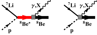
Figure 2: The Feynman diagrams for the $M1$ and $M1^{X}$ (left), and $E1$ and $E1^{X}$ (right) transitions. In the left diagram, the intermediate ${}^{8}\mathrm{Be}^{\ast}$ states are the two $1^{+}$ resonances.

The photon-production matrix element of the $J_{\gamma}^{\mu}$ operator between the initial $p$-${}^{7}\mathrm{Li}$(${3\over 2}^{-}$) system and the ${}^{8}\mathrm{Be}$ ($0^{+}$) ground state is given by $\langle^{8}\mathrm{Be};-\bm{q}|{J}_{\gamma}^{\mu}(\bm{q})|{}^{7}\mathrm{Li}+p;\,a,\,\sigma,\,\bm{p}\rangle$, with $a$ and $\sigma$ as ${}^{7}\mathrm{Li}$ and proton spin projections and $\bm{q}$ as the (virtual) photon momentum. (From now on, the physical variables in bold fonts, such as $\bm{q}$ denote 3-dimensional vectors.) This matrix element has various components, labeled by $U_{\lambda SL}$ Zhang:2017zap , with $\lambda$, $S$, and $L$ labeling the $\gamma$’s multipolarity $(\lambda)$, the total spin ($S$) and orbital angular momentum ($L)$ in the initial state.

The $\gamma$ production proceeds by either direct proton capture on ${}^{7}\mathrm{Li}$ (see the right diagram in Fig. 2) or by populating the two intermediate $1^{+}$ excited states Tilley:2002vg ; Tilley:2004zz of ${}^{8}\mathrm{Be}$ at relevant beam energies (see the left diagram in Fig. 2). The properties of the two $1^{+}$ resonances are shown in Fig. 1 and Table. 1. Since the scattering energy between $p$ and ${}^{7}\mathrm{Li}$ considered here is very low, only $s$ and $p$ wave initial states ($L=0,1$) need to be considered, while its total spin $S=1,2$. Parity and angular momentum conservation leads to selection rules that require only three amplitudes: $U_{\scriptscriptstyle 110}$ for $E1$, $U_{\scriptscriptstyle 111}$ and $U_{\scriptscriptstyle 121}$ for $M1$. The role of the $E2$ transition is negligible Zhang:2017zap and ignored here.

	$E_{\scriptscriptstyle\left(i\right)}$ (MeV)	$\Gamma_{\gamma{\scriptscriptstyle\left(i\right)}}$ (eV)	$\Gamma_{\scriptscriptstyle\left(i\right)}$ (keV)
$i=0$	0.895	$1.9(\pm 0.4)$	$138(\pm 6)$
$i=1$	0.385	$15.0(\pm 1.8)$	$10.7(\pm 0.6)$

Table 1: From the left to right: the approximate isospin ($i$), excitation energies, EM and strong decay widths of the ${}^{8}\mathrm{Be}$’s two $1^{+}$ resonances Tilley:2004zz .

The basic difference between $X$-boson and $\gamma$ production is that $M_{X}$ is non-zero (and is around 17 MeV Feng:2016jff ). Therefore, the $X$ has three independent polarizations $\tilde{\lambda}=\pm 1,0$. We follow Ref. Feng:2020mbt to apply the $q^{\mu}\varepsilon^{X}_{\mu}(q,{\tilde{\lambda}})=0$ constraint Weinberg:1995mt with $\varepsilon^{X}_{\mu}(q,{\tilde{\lambda}})$ as the polarization vector. Based on the derivation of the vector-current multipoles—as a part of the electroweak current—of many-nucleon systems [see Eqs. (7.20) (45.12) and (45.13) in Ref. Walecka:1995mi ], we can see that (1) for the transverse polarizations, the corresponding $E1^{X}$ and $M1^{X}$ multipoles are defined in the same way as $E1$ and $M1$ multipoles; (2) in addition, there are longitudinal multipoles (e.g., $L0^{X}$ and $L1^{X}$) that couples to the $\tilde{\lambda}=0$ polarization, and $J^{0}_{X}$-charge-induced multipoles ($C0^{X}$ and $C1^{X}$). Since $L$ and $C$ multipoles don’t contribute in $\gamma$ production, no direct information can be drawn for these multipoles from the $\gamma$ production data. However, in both $X$ and $\gamma$ productions, their momenta (with $\omega$ as their energy),

$$|\bm{q}|=\begin{cases}\!\sqrt{\omega^{2}-M_{X}^{2}}\sim O(1)\ \text{MeV for $X$}\\ \!\omega\sim O(10)\ \text{MeV for $\gamma$, }\end{cases}$$ (8)

are much smaller than the inverse of the nuclear length scale ($\sim O(10^{2})$ MeV). In this region, as discussed in the Appendix  A, $L1^{X}$ and $C1^{X}$ are directly related to the $E1^{X}$. In the following discussion of multipoles, we focus on the $E1$, $M1$, $E1^{X}$ and $M1^{X}$ at the $|\bm{q}|\to 0$ limit, and comment on $C0^{X}$ and $L0^{X}$ in the end.

Before going into the reaction formalism Zhang:2017zap which uses ${}^{7}\mathrm{Li}$ and $p$ as fundamental degrees of freedom, it is worth understanding the isospin structure of the $U_{\scriptscriptstyle 1SL}$ on the nucleon level. It provides the key relationship between $\gamma$ and $X$ production amplitudes.

The single-nucleon electric and magnetic multipole operators, derived from the $J^{\mu}_{\gamma}$ current in Eq. (6), are well-known (e.g., see Eqs. (5.45) and (5.71) in Ref. Lawson1980 ). The $E1$ operator is given by

$$\bm{\mathcal{O}}_{\mathrm{E}1}^{\gamma} = e_{\mathrm{EM}}\sqrt{\frac{3}{4\pi}}\sum_{i=1}^{A}\bm{r}_{(i)}\frac{\tau_{(i),3}}{2}\ .$$ (9)

The summation index ${(i)}$ labels the nucleons inside the ${}^{8}\mathrm{Be}$ system. The operator $\bm{\mathcal{O}}_{\mathrm{E}1}^{\gamma}$ is explicitly isovector. The $M1$ transitions are governed by the operator

$$\bm{\mathcal{O}}_{\mathrm{M}1}^{\gamma}= \sqrt{\frac{3}{4\pi}}\frac{e_{\mathrm{EM}}}{2M_{N}}\sum_{i}\left[\left(\lambda^{(1)}+\frac{1}{4}\right)\bm{\sigma}_{(i)}\tau_{(i),3}\right.$$

$$\left.+\left(\lambda^{(0)}+\frac{1}{4}\right)\bm{\sigma}_{(i)}+\frac{1}{2}\bm{J}_{(i)}\left(1+\tau_{(i),3}\right)\right]$$

$$\overset{\mathrm{here}}{\approx} \sqrt{\frac{3}{4\pi}}\frac{e_{\mathrm{EM}}}{2M_{N}}\sum_{i}\left[\left(\lambda^{(1)}+\frac{1}{4}\right)\bm{\sigma}_{(i)}+\frac{1}{2}\bm{J}_{(i)}\right]\tau_{(i),3}$$ (10)

$\bm{\mathcal{O}}_{\mathrm{M}1}$ is simplified in Eq. (10) based on that (1) the matrix element of the total angular momentum $\bm{J}=\sum_{i}\bm{J}_{(i)}$ (assuming the nucleus is made only of nucleons) between the initial resonances and the final state are zero, because $\bm{J}$ does not connect states with different angular momentum; and (2) numerically $|\lambda^{(1)}+\frac{1}{4}|\,(=2.10)\,\gg|\lambda^{(0)}+\frac{1}{4}|\,(=0.19)$. These expressions for $\bm{\mathcal{O}}_{\mathrm{E}1}$ and $\bm{\mathcal{O}}_{\mathrm{M}1}$ are corrected by two-body meson exchange currents that are mainly transverse and isovector Lawson1980 ; Pastore:2014oda . Therefore both $E1$ and $M1$ transitions here are isovector in nature.

As mentioned above, $E1^{X}$ and $M1^{X}$ are defined in the same way as $E1$ and $M1$ but with $J_{\gamma}^{\mu}\to J_{X}^{\mu}$ Walecka:1995mi . The resulting $E1^{X}$ and $M1^{X}$ transition operators for the $X$ production are obtained using Eq. (7) (i.e., by multiplying the isoscalar and isovector components in both $\bm{\mathcal{O}}_{\mathrm{E}1}$ and $\bm{\mathcal{O}}_{\mathrm{M}1}$ by $\varepsilon_{s}$ and $-\varepsilon_{v}$ respectively):

$$\bm{\mathcal{O}}_{\mathrm{E}1}^{X} = -\varepsilon_{v}\bm{\mathcal{O}}_{\mathrm{E}1}^{\gamma}$$ (11)

$$\bm{\mathcal{O}}_{\mathrm{M}1}^{X} = \sqrt{\frac{3}{4\pi}}\frac{e_{\mathrm{EM}}}{2M_{N}}\sum_{i}\left[-\varepsilon_{v}\left(\lambda^{(1)}+\frac{1}{4}\right)\bm{\sigma}_{(i)}\tau_{(i),3}\right.$$ (12)

$$\left.+\varepsilon_{s}\left(\lambda^{(0)}+\frac{1}{4}\right)\bm{\sigma}_{(i)}+\frac{1}{2}\bm{J}_{(i)}\left(\varepsilon_{s}-\varepsilon_{v}\tau_{(i),3}\right)\right]$$

$$= \sqrt{\frac{3}{4\pi}}\frac{e_{\mathrm{EM}}}{2M_{N}}\sum_{i}\left\{\varepsilon_{s}\left(\lambda^{(0)}+\frac{1}{4}\right)\bm{\sigma}_{(i)}\right.$$

$$\left.-\varepsilon_{v}\tau_{(i),3}\left[\left(\lambda^{(1)}+\frac{1}{4}\right)\bm{\sigma}_{(i)}+\frac{1}{2}\bm{J}_{(i)}\right]\right\}$$

$$\approx -\varepsilon_{v}\bm{\mathcal{O}}_{\mathrm{M}1}^{\gamma}$$ (13)

The approximation in Eq. (13) would only fail if the isoscalar piece in $\bm{\mathcal{O}}_{\mathrm{M}1}^{X}$ is greater or comparable than the isovector piece in size, i.e.,

$$\left|\frac{\varepsilon_{s}}{\varepsilon_{v}}\right|\gtrsim\left|\frac{\lambda^{(1)}+\frac{1}{2}}{\lambda^{(0)}+\frac{1}{4}}\right|\approx 12.$$ (14)

The ${1}/{2}$ in the $|\lambda^{(1)}+{1}/{2}|$ results from combining the spin part of the $\sum_{i}\tau_{(i),3}\bm{J}_{(i)}$ piece [$=\sum_{i}\tau_{(i),3}\left(\bm{L}_{(i)}+\bm{\sigma_{(i)}}/2\right)$] with the $\sum_{i}\tau_{(i),3}\bm{\sigma}_{(i)}$ piece; the $\bm{L}_{(i)}$ part in the former piece is neglected, because it is either $0$ or $1$ according to shell model and thus its contribution is much smaller than than that of the spin part.

Accepting the condition of Eq. (14) would require $X$-proton and -neutron to have almost the same coupling strength, which contradicts $X$ being protophobic. (Note according to Ref. Feng:2016ysn , $\varepsilon_{s}/\varepsilon_{v}\lesssim 3$.) Moreover, including the two-body current contribution to $\bm{\mathcal{O}}_{\mathrm{M}1}^{X}$ would further increase Pastore:2014oda the dominance of the isovector component over the isoscalar one, and thus makes Eq. (13) a better approximation.

In summary, the $E1^{X}$ and $M1^{X}$ operators for protophobic $X$ boson production are (to an excellent approximation) simply proportional to those for the $\gamma$ production, with an overall factor $-\varepsilon_{v}$.

Next we briefly describe our effective field theory (EFT) inspired model Zhang:2017zap for $\gamma$ production, which provides a good description of the cross section data Zahnow1995 , and the space anisotropy data Schlueter1964 ; Mainsbridge1960 . The model uses ${}^{7}\mathrm{Li}$ and $p$ as fundamental degrees of freedom to construct the appropriate Lagrangian, so that the model reproduces the properties of nuclear resonances near ${}^{7}\mathrm{Li}$-$p$ threshold, including both MIS and MIV $1^{+}$ states. Appropriate EM transition vertices are then constructed to describe both direct EM capture process and the radioactive decay of resonant states populated by ${}^{7}\mathrm{Li}$-$p$ scattering. Their Feynman diagrams can be found in Fig. 2. The former has smooth dependence on the beam energy while the latter shows resonant behavior. Both components can be qualitatively identified in the $\gamma$ production data, as shown in the top panel (purple error bars) in Fig. 3.

The next step is to separate the $E1$ and $M1$ contributions to the $\gamma$-production cross section and then use the relations in Eqs. (11) and (13) to obtain the $E1^{X}$ and $M1^{X}$ contributions to the $X$-boson production. One may immediately expect that the $E1^{X}$ contributions will be substantial if the $E1$ and $M1$ contributions are comparable. This is important because the observed enhancement of $e^{+}$-$e^{-}$pair-production is associated only with an $M1^{X}$ transition.

The differential cross section can be computed Zhang:2017zap via

$$\frac{d\sigma_{\scriptscriptstyle\gamma,X}}{d\cos\theta}=\frac{M}{4\pi}\frac{q}{p}\frac{1}{8}\sum_{a,\sigma,\tilde{\lambda}}|\mathcal{M}_{\scriptscriptstyle\gamma,X}|^{2}\ .$$ (15)

$\mathcal{M}_{\scriptscriptstyle\gamma,X}$ is the reaction amplitude depending on polarizations $\tilde{\lambda}$ and nuclear spin projections $a$ and $\sigma$; $M$ the reduced mass between ${}^{7}\mathrm{Li}$ and proton; $\theta$ the angle between boson momentum $\bm{q}$ and beam direction in the CM frame; $q\equiv|\bm{q}|$; $p\equiv\sqrt{2ME}$ ($E$ as the CM initial-state kinetic energy with $E=7/8E_{\mathrm{lab}}$). For both productions, the boson energy $\omega\equiv q^{0}=E+E_{\mathrm{th}}$ ($E_{\mathrm{th}}$ as the ${}^{7}\mathrm{Li}$-$p$ threshold energy wrt the ${}^{8}\mathrm{Be}$ ground state, see Fig. 1), ignoring the final state ${}^{8}\mathrm{Be}$’s very small recoiling energy. Note for $\gamma$, $\omega=q$, while for X, $\omega=\sqrt{M_{X}^{2}+q^{2}}$.

For $X$ production, $\sum_{\tilde{\lambda}}\varepsilon^{X}_{\mu}\varepsilon^{X}_{\nu}=-\left(g_{\mu\nu}-{q_{\mu}q_{\nu}}/{M_{X}^{2}}\right)$, since $q^{\mu}\varepsilon^{X}_{\mu}(q,{\tilde{\lambda}})=0$ Feng:2020mbt . $\sum_{a,\sigma,\tilde{\lambda}}|\mathcal{M}_{\scriptscriptstyle X}|^{2}$ becomes

$$\sum_{a\sigma\tilde{\lambda}}J_{X\mu}J_{X\nu}^{\ast}\,\varepsilon^{\mu}\varepsilon^{\nu}=\sum_{a\sigma}J_{X,i}J_{X}^{\ast\,j}\left(\delta_{j}^{i}-\frac{q_{j}q^{i}}{\omega^{2}}\right),$$ (16)

with $J$ now as the currents’ matrix elements between nuclear states and $i,j$ as the space indices. The current conservation for which $J_{X}^{0}=\bm{q}\cdot\bm{J}_{X}/\omega$ is employed in the derivation. As reasoned above, the pieces in $J_{X}^{\mu}$ corresponding to $E1^{X}$ and $M1^{X}$ can be derived by multiplying the corresponding pieces in $J_{\gamma}^{\mu}$ by $-\varepsilon_{v}$. (The latter’s expression in terms of $U_{\lambda SL}$ can be found in Eq. (3.1) in Ref. Zhang:2017zap .) In addition, Appendix A shows that the contributions of $L1^{X}$ and $C1^{X}$ associated with $E1^{X}$ are automatically included in Eq. (16) as well.

For an on-shell photon, $\omega=q$, so the above formula also applies for $\sum_{a,\sigma,\tilde{\lambda}}|\mathcal{M}_{\scriptscriptstyle\gamma}|^{2}$ with $J_{X}^{\mu}\to J_{\gamma}^{\mu}$.

The net result, including ($E1$, $M1$) and ($E1^{X}$, $L1^{X}$, $C1^{X}$, $M1^{X}$) multipoles and evaluating the spin sums, is to arrive at the following decomposition:

$$\sum_{a,\sigma,\tilde{\lambda}}|\mathcal{M}_{\scriptscriptstyle\gamma,X}|^{2}=T_{0}^{\scriptscriptstyle\gamma,X}+T_{1}^{\scriptscriptstyle\gamma,X}\,P_{1}\left(\cos\theta\right)+T_{2}^{\scriptscriptstyle\gamma,X}\,P_{2}\left(\cos\theta\right),$$

where, $P_{n}$ are the Legendre polynomials, and

$$T_{0}^{X}/\varepsilon_{v}^{2} =(3\omega^{2}-{q}^{2})|U_{\scriptscriptstyle 110}|^{2}+\frac{2}{3}{q}^{2}\left(\frac{p}{M}\right)^{2}\bigg{[}|U_{\scriptscriptstyle 111}|^{2}+|U_{\scriptscriptstyle 121}|^{2}\bigg{]}\ ,$$ (18)

$$T_{1}^{X}/\varepsilon_{v}^{2} =2\sqrt{2}\omega q\left(\frac{p}{M}\right)\,\mathrm{Im}\left(U_{\scriptscriptstyle 111}U_{\scriptscriptstyle 110}^{\ast}\right)\ ,$$ (19)

$$T_{2}^{X}/\varepsilon_{v}^{2} =\frac{1}{3}q^{2}\left(\frac{p}{M}\right)^{2}\bigg{[}|U_{\scriptscriptstyle 111}|^{2}-\frac{1}{5}|U_{\scriptscriptstyle 121}|^{2}\bigg{]}\ .$$ (20)

Expressions for $T_{n}^{\gamma}$ (that agree with those in Ref. Zhang:2017zap ) are obtained from the above formula by using $q=\omega$ and setting $\varepsilon_{v}$ to unity.

Expressions for $U_{\lambda SL}$ in terms of EFT coupling parameters are Eqs. (3.2), (3.5) and (3.6) in Ref. Zhang:2017zap . The parameters are fixed by reproducing the photon production data, including total cross section, and ${T_{1}^{\gamma}}/{T^{\gamma}_{0}}$ and ${T_{2}^{\gamma}}/{T^{g}_{0}}$ ratios, with $E_{\mathrm{lab}}\equiv{8}/{7}E$ below 1.5 MeV. Note the amplitudes $U_{\lambda SL}$ depend only on $E$, but not $\omega$ or $q$.

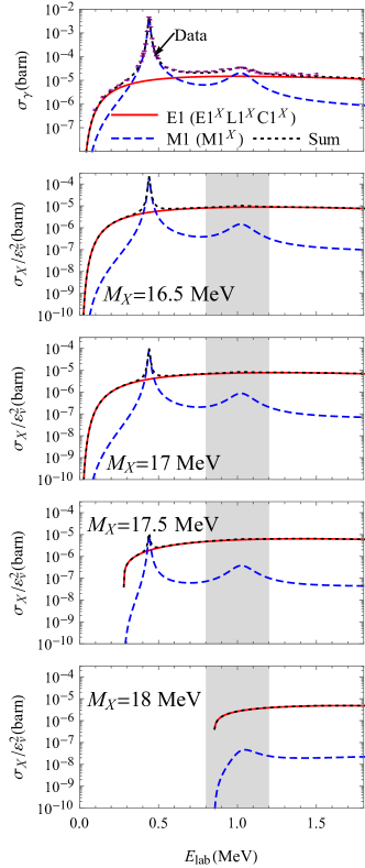
Figure 3: Top: $\sigma_{\gamma}$ vs. the proton’s lab energy $E_{\mathrm{lab}}$. The data are from Ref. Zahnow1995 . The lower panels: $\sigma_{X}/\varepsilon_{v}^{2}$ for different values of $M_{X}$. The shaded regions cover the four measured energies Krasznahorkay:2015iga . The legends are shared by all the panels; $E1$ ($E1^{X}$ $L1^{X}$ $C1^{X}$), $M1$ ($M1^{X}$), and their sum are shown as sold (red), dashed (blue), and dotted (black) lines.

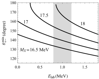
Figure 4: The minimum values of the pair correlation angles vs. the proton’s lab energy $E_{\mathrm{lab}}$. Four different cases are plotted with the corresponding masses indicated. The shaded regions again cover the four measured energies Krasznahorkay:2015iga .

We now turn to the results, starting with the $\gamma$-production cross section shown in the upper panel of Fig. 3. The model provides good agreement with the data from Ref. Zahnow1995 . For further comparisons between theory and experiment see Ref. Zhang:2017zap . The salient features are the two $M$1 resonance contributions, with the lower-energy MIV peak being much higher, and the smooth behavior of those of the $E1$. Except for the strong peaks at the two $1^{+}$ resonances, the $E1$ dominates.

The resonance peaks occur from a two-step process in which the strong interaction connects the initial $|{}^{7}\mathrm{Li},p\rangle$ to the 1⁺ states which then decay by emitting a photon (see the left diagram in Fig. 2). The relative strengths of the two peaks naturally arise from Eq. (10). If the 1⁺ states were pure isospin eigenstates, the $\bm{\mathcal{O}}_{\mathrm{M}1}$ operator would only connect the lower-energy state with the ground state. $\gamma$-production at the higher-energy resonance occurs only because isospin mixing between the two 1⁺ states causes the higher-energy state to have an isospin 1 amplitude of $-0.21$ Pastore:2014oda ; Wiringa:2013fia . The kinematics together with this ratio can qualitatively explain the ratio of photon widths $\Gamma_{\gamma{\scriptscriptstyle\left(i\right)}}$ listed in Table 1 Feng:2016ysn . The difference between the strong decay widths shown in that Table arises from phase space factors and the greater importance of the Coulomb barrier at lower energies Zhang:2017zap . The final $|{}^{7}\mathrm{Li},p\rangle$ states in these strong decays are equal mixtures of isospin 0 and 1, so the 1⁺ states’ isospin contents do not dictate the strong decay width.

Next turn to the production of $X$ bosons. Eq. (18) gives the relative magnitude of the total $X$ production cross section i.e., $\sigma_{X}/\varepsilon_{v}^{2}$ and its decomposition into the $ELC1^{X}$ and $M1^{X}$ components. (From now on, $ELC1^{X}$ means the combination of $E1^{X}$, $L1^{X}$ and $C1^{X}$, since they always show up together.) The first term, being proportional to $3\,\omega^{2}-q^{2}$, is $ELC1^{X}$ contributions (for the photon this factor is $2\omega^{2}$). The second term gives that of $M1^{X}$, whose $q^{2}$ factor arises from the magnetic nature of the interaction.

The results thus obtained for four different $M_{X}$ (16.5, 17, 17.5 18 MeV) around the suggested values from Ref. Feng:2016jff are shown in the lower four panels of Fig. 3. The shaded regions cover the four different $E_{\mathrm{lab}}$ values, $0.8,1.04,1.1,1.2$ MeV, that have been measured by the experiment Krasznahorkay:2015iga . The $X$ can be produced via the dominant $ELC1^{X}$ component for almost any energy above the kinematic threshold, except around the MIV resonance for $M_{X}=16.5$, $17$ and $17.5$ MeV. (The ${}^{7}\mathrm{Li}$-$p$ threshold is $17.26$ MeV above ${}^{8}\mathrm{Be}$’s ground state, and thus no kinetic threshold exists for $M_{X}=16.5$, $17$ and $17.5$ MeV, while such threshold for $M_{X}=18$ MeV eliminates $X$ production around the MIV resonance.)

One key experimental signal of the $X$ productions is the enhanced $e^{+}$-$e^{-}$detection—from $X$’s decay—in the region of large pair-correlation-angle ($\theta_{\scriptscriptstyle+-}$) as measured in the lab frame, on the top of the EM-induced pair production background that varies smoothly in the same region Krasznahorkay:2015iga ; Zhang:2017zap . If $M_{X}\approx\omega$, $\theta_{\scriptscriptstyle+-}$ is limited to a small window, between $\theta_{\scriptscriptstyle+-}^{\mathrm{min}}$ and $180^{\circ}$, which can be seen based on heavy-particle-decay kinematics (see Ref. Feng:2020mbt ). Fig. 4 plots $\theta_{\scriptscriptstyle+-}^{\mathrm{min}}$ against $E_{\mathrm{lab}}$ for the four different $M_{X}$ values. For example, with $M_{X}=17$ MeV and $0.8\leq E_{\mathrm{lab}}\leq 1.2$ MeV (shaded region), the $X$-decay $e^{+}$-$e^{-}$are concentrated in $140^{\circ}\leq\theta_{\scriptscriptstyle+-}\leq 180^{\circ}$; while for other masses, $\theta_{\scriptscriptstyle+-}$s are in qualitatively similar regions.

Since the full $X$-production cross section varies smoothly with $E_{\mathrm{lab}}$ as shown in Fig. 3, the enhanced $e^{+}$-$e^{-}$detection in the $\theta_{\scriptscriptstyle+-}\sim 180^{\circ}$ region should have been observed across the shaded region. This is in direct conflict with the experimental observation of such enhancement associated only with the higher energy 1⁺ state, i.e., not seen at $E_{\mathrm{lab}}=0.8$ and $1.2$ MeV Krasznahorkay:2015iga .

The dominance of the $ELC1^{X}$ component around the MIS resonance and the strong dependence of the $ELC1^{X}/M1^{X}$ ratio on the value of $M_{X}$, as shown in the figure can be understood using a simple calculation. The ratio can be inferred from the same ratio for the $\gamma$ production (the phase space factors canceled in the ratios). At a given beam energy $E$,

$$\frac{\sigma_{X,ELC1^{X}}(E)}{\sigma_{X,M1^{X}}(E)}=\frac{\sigma_{\gamma,E1}(E)}{\sigma_{\gamma,M1}(E)}\frac{3\omega^{2}-q^{2}}{2q^{2}}\ ,$$ (21)

with $\omega$ as energy for both $X$ and photon, with $q=\sqrt{\omega^{2}-M_{X}^{2}}$. Now, at the energy of the MIS resonance where the anomaly was observed, Fig. 3 shows $\sigma_{\gamma,E1}\approx 0.7\ \sigma_{\gamma,M1}$. Here $\omega=18.15$ MeV, and $q=6.36$ MeV for $M_{X}=17$ MeV. Then Eq. (21) tells us that

$$\left.\frac{\sigma_{X,ELC1^{X}}}{\sigma_{X,M1^{X}}}\right|_{MIS}=\frac{2\omega^{2}+M_{X}^{2}}{2(\omega^{2}-M_{X}^{2})}\left.\frac{\sigma_{\gamma,E1}}{\sigma_{\gamma,M1}}\right|_{MIS}\overset{M_{X}=17}{\approx}8.6\ .$$

The sensitivity to the value of $M_{X}$ can be seen from the denominator—$M_{X}$ is close to $\omega$.

The ratio 8.6 is obtained by assuming that Eq. (13) is exact. However to evade this conclusion, $|\varepsilon_{s}/\varepsilon_{v}|$ must be around or larger than $12$ as shown in Eq. (14), which conflicts with $X$ being protophobic.

In summary, the results presented in Fig. 3 show that there would be a signal of $X$ production due to the $E1^{X}+L1^{X}+C1^{X}$ transitions, i.e., Bremsstrahlung radiation of $X$ boson at all beam energies above threshold. This mechanism has a smooth beam energy $E_{\mathrm{lab}}$ dependence, while the resonant production diminishes quickly when $E_{\mathrm{lab}}$ is a few widths away from the resonances. In fact, given a 17 MeV $X$ boson, the enhancement signal should have been seen at all four of energies of the ATOMKI experiment Krasznahorkay:2015iga . For a $18$ MeV $X$ boson, although $X$ production around the MIV resonance is eliminated due to kinematic threshold, the smooth Bremsstrahlung component should still be detectable above the MIS resonance. However, the experimental observation Krasznahorkay:2015iga of the anomaly is absent below or above the MIS, higher-energy 1⁺, resonance. Therefore, the explanation of the anomaly in terms of protophobic vector boson $X$ cannot be correct.

It is worth commenting on the $C0^{X}$ and $L0^{X}$ multipoles which contribute to the $X$-production but not to the $\gamma$ production. Although their contributions can not be inferred from the $\gamma$ production, their energy dependences are smooth, because they do not induce transition between ${}^{8}\mathrm{Be}$’s $1^{+}$ resonance and $0^{+}$ ground state. Therefore, their contributions enhance the smooth-energy-dependence component in the $X$-production cross section, which further strengthens our basic conclusion.

Our considerations here are concerned with the $A=8$ system. However, for the $A=4$ system ⁴He, where a signal of $X$-boson production has also been claimed Feng:2020mbt ; Krasznahorkay:2019lyl , the Bremsstrahlung terms induced by the ($L0^{X}$, $C0^{X}$) multipoles, and the $ELC1^{X}$ induced resonant productions from the two $1^{+}$ resonances—about $3.5$ MeV above the experimental measurement Krasznahorkay:2019lyl but with about $6$ MeV widths Tilley:1992zz —will be present. Therefore, given the coupling constants of Ref. Feng:2020mbt one should reasonably expect to have seen a signal at all beam energies. Detailed nuclear calculations of the $L0^{X}$, $C0^{X}$, $E1^{X}$, $L1^{X}$ and $C1^{X}$ matrix elements for $A=4$ would be valuable for addressing this issue.

Appendix A Multipoles for producing a massive vector boson

The reaction amplitude for producing a photon $\gamma$ or $X$ is

$$\mathcal{M}_{\gamma,X}=-e_{\mathrm{EM}}\varepsilon^{\gamma,X}_{\mu}\langle f|j^{\mu}_{\gamma,X}|i\rangle\ ,$$ (23)

with $|i(f)\rangle$ as nuclear states and $j^{\mu}_{\gamma,X}$ currents defined in Eqs. (1) and (2). Two different ways are employed to describe these amplitudes with $\gamma$ and $X$’s $|\bm{q}|\to 0$.

From a low-energy EFT perspective, the $\gamma$ and $X$ fields $A_{\mu}$ and $X_{\mu}$ can be treated as external fields Gasser:1983yg in constructing an effective lagrangian. Based on the conservation of $j^{\mu}_{\gamma,X}$, the lagrangian density with external fields is invariant under the corresponding local symmetry transformation Gasser:1983yg . The leading order contact terms for producing a $\gamma$ can be expressed as $\hat{\bm{d}}_{\gamma}\cdot(\partial_{t}\bm{A}-\bm{\partial}A_{0})$ for the $E1$, and $\hat{\bm{\mu}}_{\gamma}\cdot(\bm{\partial}\times\bm{A})$ for the $M1$. $\hat{\bm{d}}_{\gamma}$ and $\hat{\bm{\mu}}_{\gamma}$ are electric and magnetic dipole operators, which can be expressed in terms of nuclear cluster fields. For example, in Eqs. (2.4) and (2.5) in the Ref. Zhang:2017zap , both operators are constructed using ⁷Li and proton fields. The lagrangian terms for $X$ production take the same forms: $\hat{\bm{d}}_{X}\cdot(\partial_{t}\bm{X}-\bm{\partial}X_{0})$ and $\hat{\bm{\mu}}_{X}\cdot(\bm{\partial}\times\bm{X})$, due to the local transformation invariance. The $\hat{\bm{\mu}}_{X}$ term again corresponds to the $M1^{X}$, but the $\hat{\bm{d}}_{X}$ term now has the $E1^{X}$ $L1^{X}$ and $C1^{X}$ contributions, since $X$ is massive. Therefore in Eq. (16), $\langle f|j^{\mu}_{X}|i\rangle$, as derived from $\langle f|\hat{\bm{d}}_{X}|i\rangle$ and $\langle f|\hat{\bm{\mu}}_{X}|i\rangle$, automatically includes the $E1^{X}$ $L1^{X}$ and $C1^{X}$’s contributions together and the $M1^{X}$’s respectively.

Note the basic argument of this paper is that $\hat{\bm{d}}_{X}$ and $\hat{\bm{\mu}}_{X}$ are proportional to $\hat{\bm{d}}_{\gamma}$ and $\hat{\bm{\mu}}_{\gamma}$ respectively because of the dominance of the isovector component.

On the nucleon level, the electroweak current multipoles have been derived in Ref. Walecka:1995mi . The vector current mulitpoles, including transverse $E^{X}$ and $M^{X}$, longitudinal $L^{X}$, and the charge-induced $C^{X}$ [Eqs. (45.12) and (45.13) in Ref. Walecka:1995mi ], can be directly applied here for the $X$ production. By comparing the ($E^{X}$, $M^{X}$) to the ($E$ $M$) defined in the Eq. (7.20) of Ref. Walecka:1995mi , we see that they can be changed into each other by $j_{X}^{\mu}\leftrightarrow j_{\gamma}^{\mu}$. Moreover, the $|\bm{q}|\to 0$ limits of these multipoles are in the Eqs. (45.35)–(45.37) of Ref. Walecka:1995mi . It can be easily checked that in this limit, the relationship between $E1^{X}$ and ($L1^{X}$, $C1^{X}$) are those given by the effective interaction $\hat{\bm{d}}_{X}\cdot(\partial_{t}\bm{X}-\bm{\partial}X_{0})$ discussed above. I.e., this effective coupling includes all the contributions from the $E1^{X}$ $L1^{X}$ and $C1^{X}$ multipoles.

References

- (1) A. J. Krasznahorkay et al., Phys. Rev. Lett. 116, no. 4, 042501 (2016).
- (2) D. R. Tilley, J. H. Kelley, J. L. Godwin, D. J. Millener, J. E. Purcell, C. G. Sheu and H. R. Weller, Nucl. Phys. A 745, 155 (2004).
- (3) J. L. Feng, B. Fornal, I. Galon, S. Gardner, J. Smolinsky, T. M. P. Tait and P. Tanedo, Phys. Rev. Lett. 117, no. 7, 071803 (2016);
- (4) B. Fornal, Int. J. Mod. Phys. A 32, 1730020 (2017) doi:10.1142/S0217751X17300204; L. B. Jia and X. Q. Li, Eur. Phys. J. C 76, no. 12, 706 (2016); U. Ellwanger and S. Moretti, JHEP 1611, 039 (2016) ; C. S. Chen, G. L. Lin, Y. H. Lin and F. Xu, Int. J. Mod. Phys. A 32, no.31, 1750178 (2017); M. J. Neves and J. A. Helayël-Neto, arXiv:1611.07974 [hep-ph]; J. Kozaczuk, D. E. Morrissey and S. R. Stroberg, Phys. Rev. D 95, no.11, 115024 (2017); P. H. Gu and X. G. He, Nucl. Phys. B 919, 209-217 (2017) doi:10.1016/j.nuclphysb.2017.03.023 ; Y. Liang, L. B. Chen and C. F. Qiao, Chin. Phys. C 41, no.6, 063105 (2017) doi:10.1088/1674-1137/41/6/063105; T. Kitahara and Y. Yamamoto, Phys. Rev. D 95, no.1, 015008 (2017) doi:10.1103/PhysRevD.95.015008 ; Y. Kahn, G. Krnjaic, S. Mishra-Sharma and T. M. P. Tait, JHEP 05, 002 (2017) doi:10.1007/JHEP05(2017)002 ; O. Seto and T. Shimomura, Phys. Rev. D 95, no.9, 095032 (2017) doi:10.1103/PhysRevD.95.095032 ; P. Fayet, Eur. Phys. J. C 77, no.1, 53 (2017) doi:10.1140/epjc/s10052-016-4568-9 ; N. V. Krasnikov, arXiv:1702.04596 [hep-ph]; L. Delle Rose, S. Khalil and S. Moretti, Phys. Rev. D 96, no.11, 115024 (2017) doi:10.1103/PhysRevD.96.115024 ; D. S. M. Alves and N. Weiner, JHEP 07, 092 (2018) doi:10.1007/JHEP07(2018)092 ; L. Delle Rose, S. Khalil, S. King, J.D., S. Moretti and A. M. Thabt, Phys. Rev. D 99, no.5, 055022 (2019) doi:10.1103/PhysRevD.99.055022 ; C. Y. Chen, D. McKeen and M. Pospelov, Phys. Rev. D 100, no.9, 095008 (2019) doi:10.1103/PhysRevD.100.095008 ; C. H. Nam, Eur. Phys. J. C 80, no.3, 231 (2020) doi:10.1140/epjc/s10052-020-7794-0 ; C. Hati, J. Kriewald, J. Orloff and A. M. Teixeira, JHEP 07, 235 (2020) doi:10.1007/JHEP07(2020)235 ; O. Seto and T. Shimomura, [arXiv:2006.05497 [hep-ph]].
- (5) J. L. Feng, B. Fornal, I. Galon, S. Gardner, J. Smolinsky, T. M. P. Tait and P. Tanedo, Phys. Rev. D 95, no.3, 035017 (2017) doi:10.1103/PhysRevD.95.035017 [arXiv:1608.03591 [hep-ph]].
- (6) J. L. Feng, T. Tait, M.P. and C. B. Verhaaren, Phys. Rev. D 102, no.3, 036016 (2020) doi:10.1103/PhysRevD.102.036016 [arXiv:2006.01151 [hep-ph]].
- (7) G. A. Miller, B. M. K. Nefkens and I. Slaus, Phys. Rept. 194, 1-116 (1990) doi:10.1016/0370-1573(90)90102-8
- (8) G. A. Miller, A. K. Opper and E. J. Stephenson, Ann. Rev. Nucl. Part. Sci. 56, 253-292 (2006) doi:10.1146/annurev.nucl.56.080805.140446 [arXiv:nucl-ex/0602021 [nucl-ex]].
- (9) G. A. Miller, Phys. Rev. C 57, 1492-1505 (1998) doi:10.1103/PhysRevC.57.1492 [arXiv:nucl-th/9711036 [nucl-th]]
- (10) F. Halzen and A. D. Martin, Quarks and Leptones: An Introductory Course in Modern Particle Physics, John Willey & Sons (New York), 1984.
- (11) X. Zhang, K. M. Nollett and D. R. Phillips, Phys. Lett. B 751, 535 (2015); EPJ Web Conf. 113, 06001 (2016); Phys. Rev. C 89, no. 5, 051602 (2014); Phys. Rev. C 89, no. 2, 024613 (2014) .
- (12) X. Zhang and G. A. Miller, Phys. Lett. B 773, 159-165 (2017) doi:10.1016/j.physletb.2017.08.013 [arXiv:1703.04588 [nucl-th]].
- (13) D. R. Tilley, C. M. Cheves, J. L. Godwin, G. M. Hale, H. M. Hofmann, J. H. Kelley, C. G. Sheu and H. R. Weller, Nucl. Phys. A 708, 3 (2002).
- (14) S. Weinberg, Section 5.3, The Quantum theory of fields. Vol. 1: Foundations, Cambridge University Press, 2005.
- (15) B. Kors and P. Nath, Phys. Lett. B 586, 366-372 (2004) doi:10.1016/j.physletb.2004.02.051 [arXiv:hep-ph/0402047 [hep-ph]].
- (16) J. D. Walecka, Theoretical nuclear and subnuclear physics, Oxford University Press, 1995.
- (17) R. D. Lawson, Theory of The Nuclear Shell Model, (1980) Oxford University Press .
- (18) S. Pastore, R. B. Wiringa, S. C. Pieper and R. Schiavilla, Phys. Rev. C 90, no. 2, 024321 (2014)
- (19) D. Zahnow, C. Angulo, C. Rolfs, S. Schmidt, W. H. Schulte, and E. Somorjai, Z. Phys. A 351, 229 (1995) .
- (20) D. J. Schlueter, R. W. Krone, and F. W. Prosser, Nucl. Phys. 58, 254 (1964) .
- (21) B. Mainsbridge, Nucl. Phys. 21, l (1960) .
- (22) R. B. Wiringa, S. Pastore, S. C. Pieper and G. A. Miller, Phys. Rev. C 88, no. 4, 044333 (2013)
- (23) A. J. Krasznahorkay, M. Csatlós, L. Csige, J. Gulyás, M. Koszta, B. Szihalmi, J. Timár, D. S. Firak, Á. Nagy, N. J. Sas and G. Cern, [arXiv:1910.10459 [nucl-ex]].
- (24) D. R. Tilley, H. R. Weller and G. M. Hale, Nucl. Phys. A 541, 1-104 (1992) doi:10.1016/0375-9474(92)90635-W
- (25) J. Gasser and H. Leutwyler, Annals Phys. 158, 142 (1984) doi:10.1016/0003-4916(84)90242-2