Isotropic Cellular Automata:
the DDLab iso-rule paradigm

Abstract

To respect physics and nature, cellular automata (CA) models of self-organisation, emergence, computation and logical universality should be isotropic, having equivalent dynamics in all directions. We present a novel paradigm, the iso-rule, a concise expression for isotropic CA by the output table for each isotropic neighborhood group, allowing an efficient method of navigating and exploring iso-rule-space. We describe new functions and tools in DDLab to generate iso-groups and iso-rules, for multi-value as well as binary, in one, two and three dimensions. These methods include filing, filtering, mutating, analysing dynamics by input-frequency and entropy, identifying the critical iso-groups for glider-gun/eater dynamics, and automatically classifying iso-rule-space. We illustrate these ideas and methods for two dimensional CA on square and hexagonal lattices.

keywords: DDLab, cellular automata, isotropy, iso-groups, iso-rules, glider-guns, logical universality, input-frequency, filtering, mutation.

1 Introduction

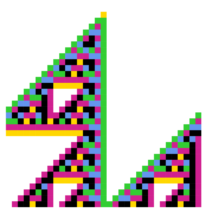
(a) the unslanted initial view

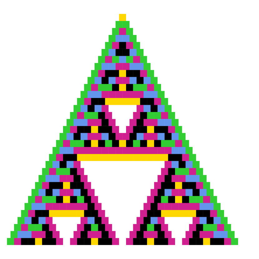
(b) time-steps shifted 1/2 cell right

Figure 1: 1d $v8k2$ space-time pattern of an isotropic CA, size 33, The rcode size=64, The iso-rule (size=36): 140761540026777563655513706072505220, as a graphic: and in hexadecimal: 07 07 c6 c0 16 ff dc f5 b4 be 30 ea 8a 90. (a) is the initial view because even n-templates are skewed right (figure 6). (b) successive time-steps shifted 1/2 cell right to restore symmetry[27, EDD:32.9.1].

Isotropy, rotational invariance, equivalence, lack of directional bias or preference arguably underlie physics and nature at the most basic level. By contrast, an isotropic “physics” of a cellular autamata universe belongs in a special and very limited category in the entirety of CA rule-spaces. As in the game-of-Life[6], Precursor[9], Spiral[2] and other comparable rules discussed in this paper, equivalent dynamics in all directions and orientations seems a proper constraint for CA models of self-organisation, emergence, computation and logical universality, where a glider-gun and its rotations/reflections work equivalently.

A counter example is the anisotropic X-rule[8, 12] which has an operational glider-gun only when orientated East-West — the same structure rotated $90^{\circ}$ becomes a simple reflector. Despite the interesting glider-guns and logical-gates created in the X-rule, its anisotropic behaviour seems unnatural.

CA rule-spaces in general are not isotropic, where rules are defined by rule-tables of length $v^{k}$ where $v$=value-range and $k$=neighborhood size, with a rule-space size of $v^{v^{k}}$. Isotropic rules, also recognisable in that symmetric patterns must conserve symmetry as time evolves — as from singleton seeds in figures 1 and 3 — make up a tiny proportion of a general rule-space.

Although some rule categories, survival/birth, totalistic, reaction-diffusion, are isotropic by default, these iso-subsets can be transformed into a general expression of isotropic CA, where the “iso-groups” of equivalent neighborhoods by all possible spins and flips share the same output — figure 2 gives examples.

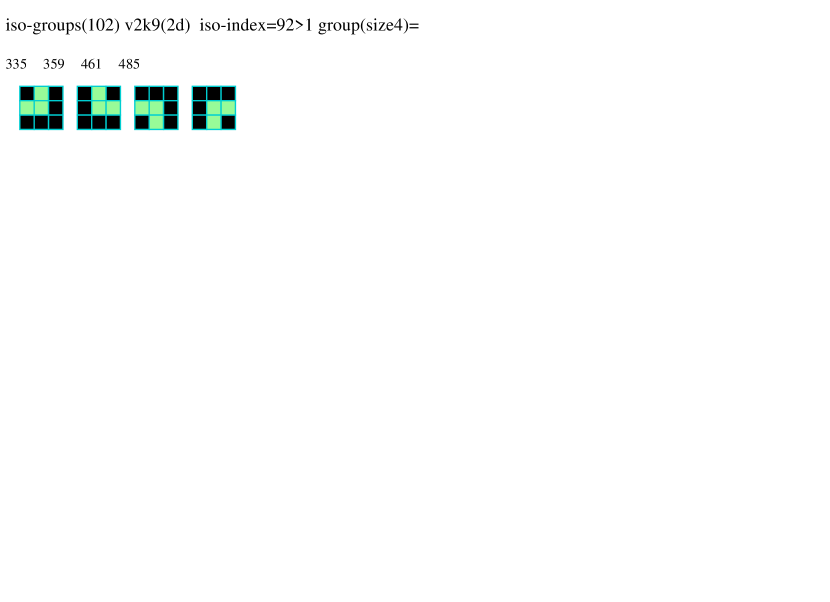
(a) 2d $v2k8$ (92/101)

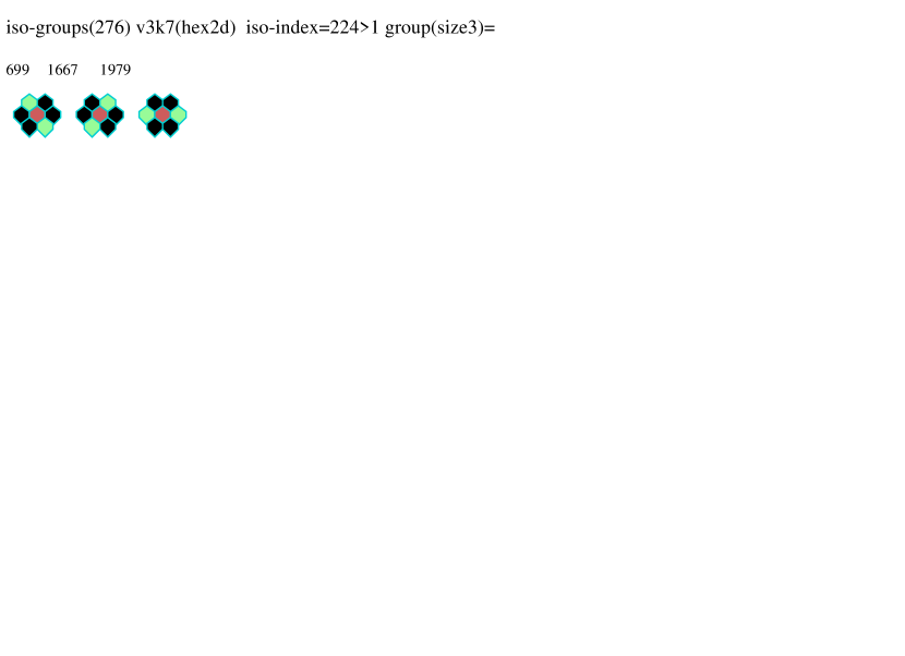
(b) 2d hex (224/275)

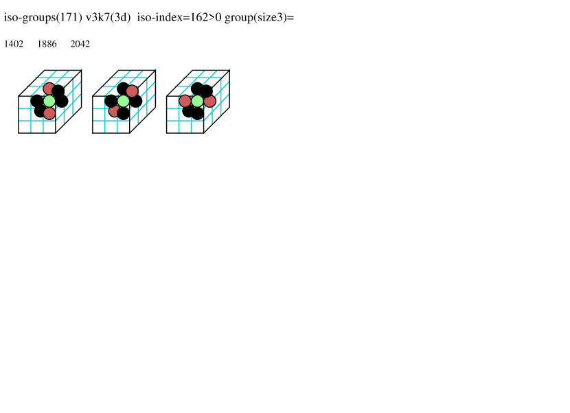
(b) 3d (162/170)

Figure 2: Examples of iso-groups showing (group-index/max-index).

Especially significant are iso-rules analogous to Conway’s famous survival/birth game-of-Life[3, 6], the first rule with logical gates constructed from glider/eater dynamics made with the first glider-gun discovered by Gosper. Figure 4 illustrates Life and other significant rules, including glider-gun iso-rules not based on survival/birth where logical universality has been demonstrated.

$v4k4$ hex 2d

$v4k6$ hex 2d

$v4k4s$ square 2d

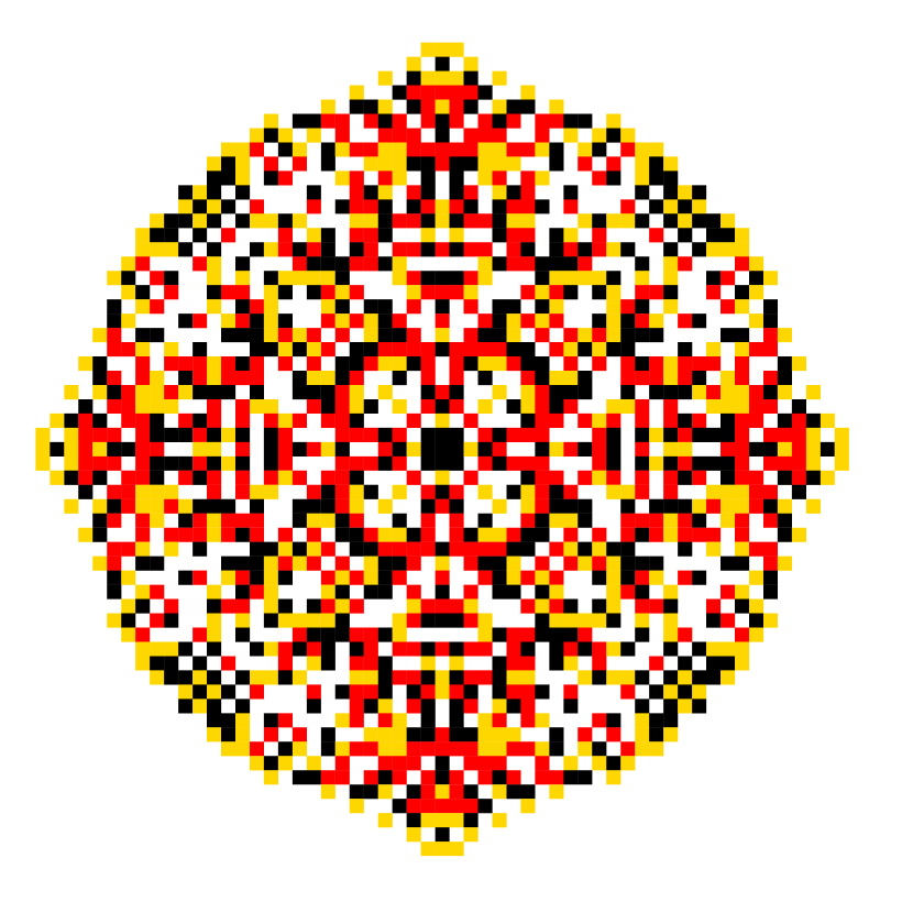
$v4k5s$ square 2d

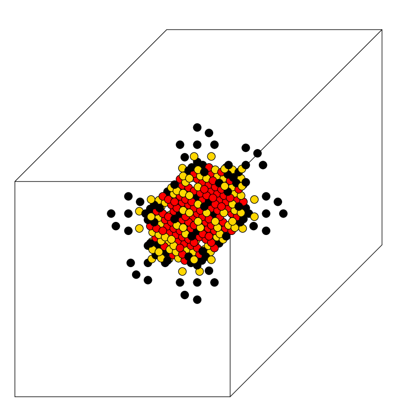
$v5k6$ cubic 3d

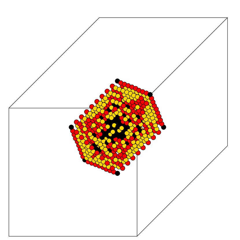
$v5k7$ cubic 3d

Figure 3: Examples of space-time pattern snapshots for $v$=4 2d and 3d isotropic CA from a singleton seed, a $v$$>$0 single cell against a zero background. The initial symmetry must be preserved. Isotropic CA, where rotated and reflected neighborhoods have the same output, are arguably closer to natural physics.

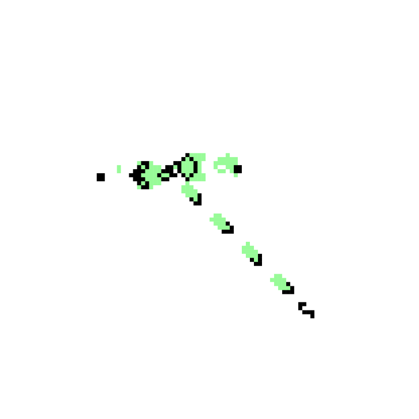
Life[3, 6]: $p$=30

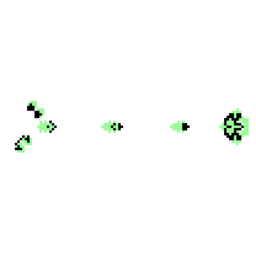
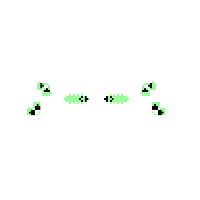
Eppstein[5]: $p$=68

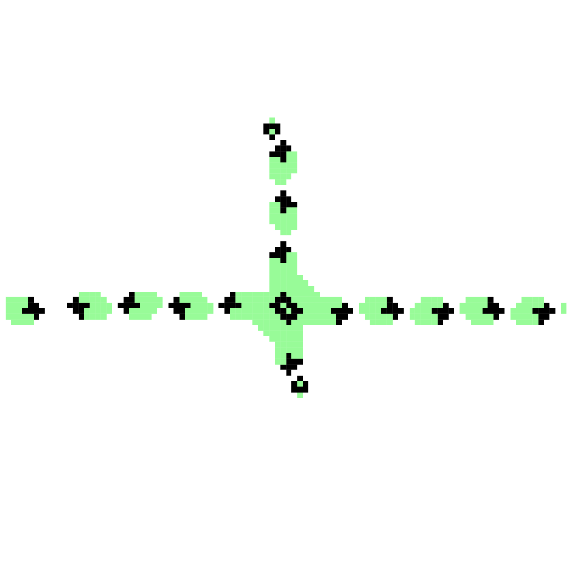
Sapin[14]: $p$=18

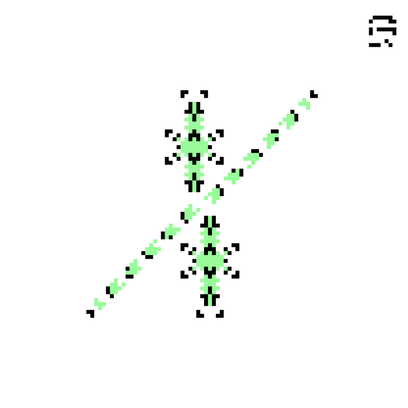
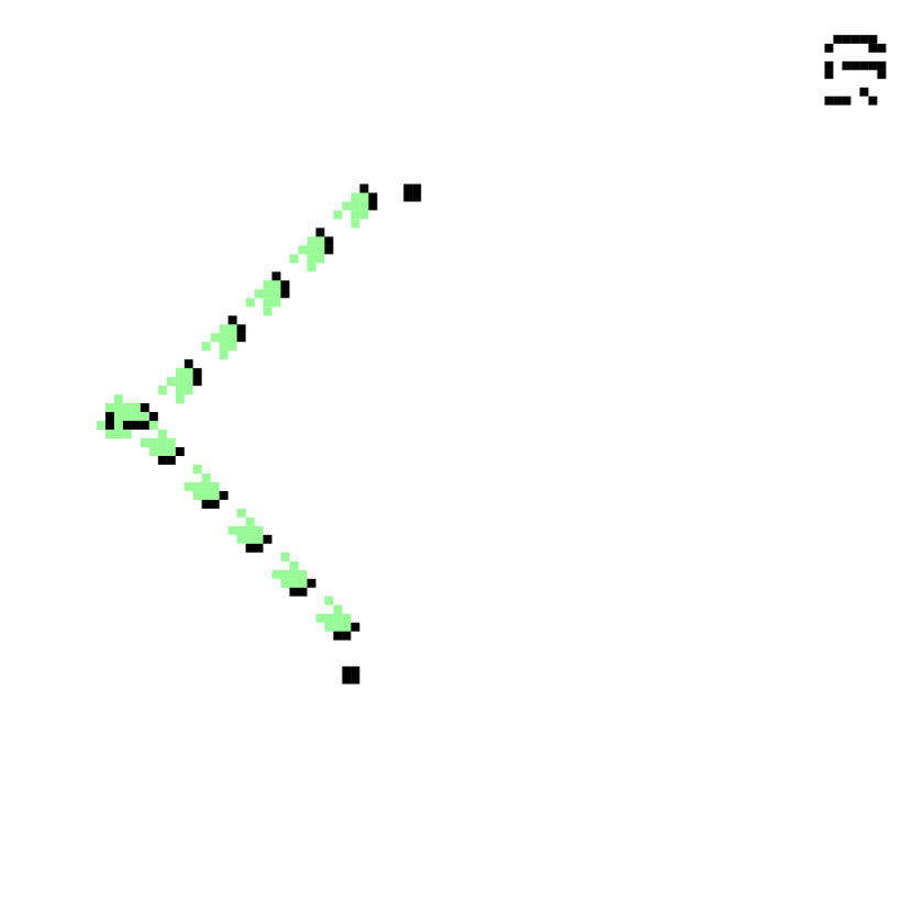
(a) Conway’s survival/birth (s23/b3) game-of-Life[3, 6] and Eppstein’s s236/b3 rule[5]. Sapin’s R-rule[14] evolved by genetic algorithm from iso-groups. Life and SapinR are logically universal with glider streams stopped by eaters, Eppstein’s by head-on collisions only — lower panel.
00 00 00 00 00 60 03 1c 61 c6 7f 86 a0 — Life
04 89 86 1a 00 6d 23 1e 61 e6 7f 86 a0 — Eppstein
11 34 1c 2c 52 36 7d 3b e0 f8 7e 0a a0 — SapinR
L E R
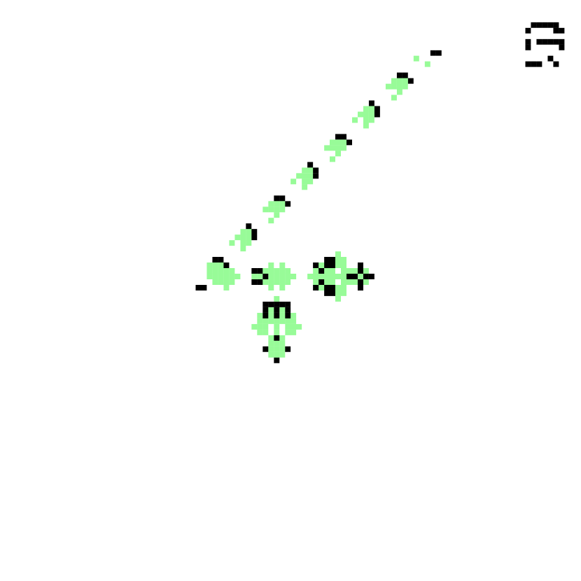
Variant[11]: $p$=22 Precursor[9]: $p$=19 Sayab[10]: $p$=20
(b) Three binary logically universal iso-rules[12] belong to a family with different glider-guns. Gliders streams are stopped by eaters. The Variant[11] and Precursor[9] rules are closely related differing by two outputs. The Sayab rule[10] is a distant cousin differing from the Precursor by 33 outputs.
24 c0 04 42 83 01 80 2c a4 29 04 e0 70 — Variant
24 c0 04 42 83 01 80 24 a4 69 04 e0 70 — Precursor
24 01 13 1a 14 20 50 2c 45 05 48 e0 50 — Sayab
V P S

Figure 4: Significant binary ($v2k9$) glider-gun iso-rules on 3$\times$3 Moore n-templates with 102 iso-groups. The iso-rule’s hexadecimal and bit expressions allow comparison of bit differences/similarities. The glider-guns in SapinR and the Sayab rule emerge spontaneously, the others are elaborately constructed artifacts. $p$=glider-gun period and firing frequency. Green trails denote motion.

(a) v3k3x1.vco, g1

(hex)00a864

(b) v3k4t1.vco, g1

(hex)2a945900

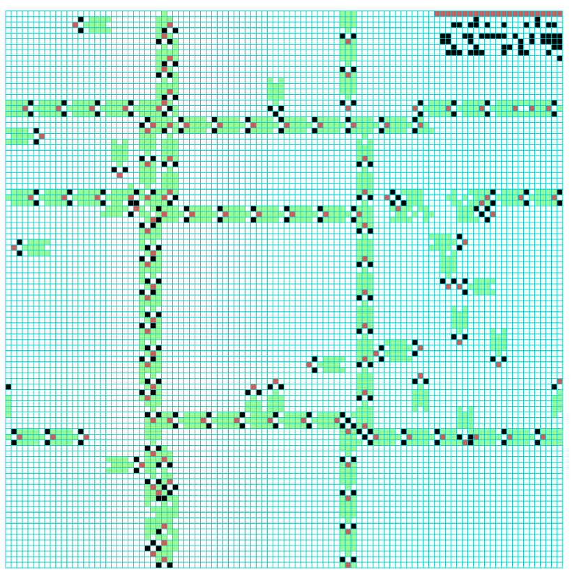
(c) v3k4x1.vco

(hex)2282a1a4

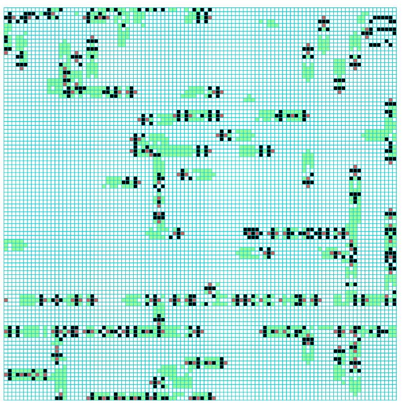
(d) v3k5x1.vco, g1

(hex)004a8a2a8254

xx

(e) v3k6n6.vco, g16

(hex)01059059560040

xx

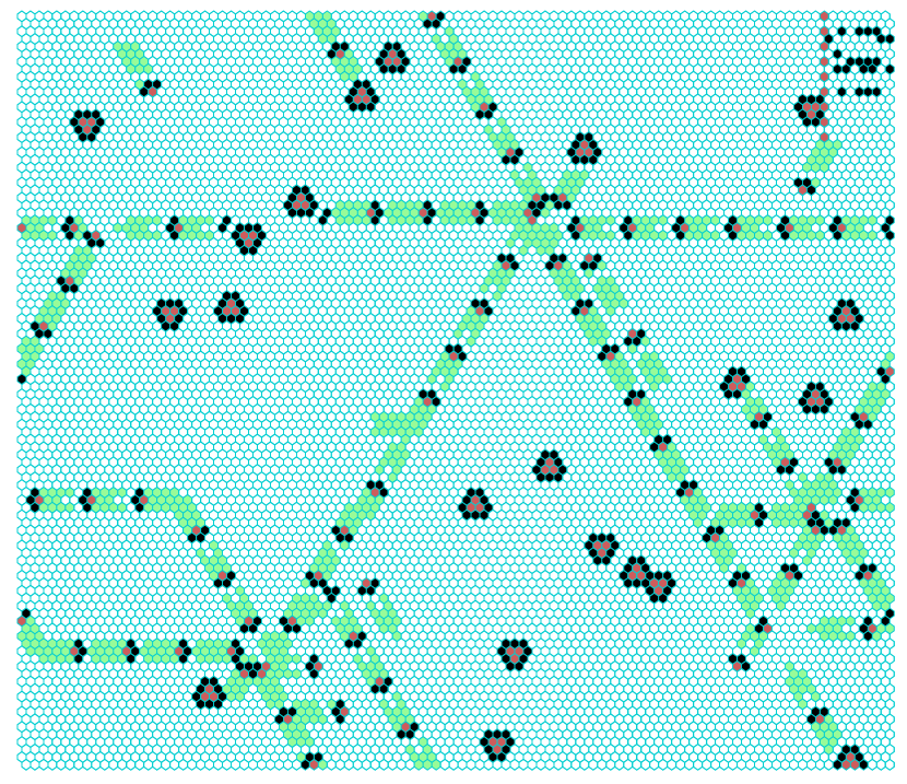
(f) v3k7w1.vco, g1

(hex)020609a2982a68aa64

The Spiral rule[24]

Figure 5: Glider dynamics discovered in 3-value 2d k-totalistic rules, on n-templates $k$=3 to 7, in figure 7. Cell values: 0=white, 1=red, 2=black. Green trails indicate motion. Examples b, c, e, and f include glider-guns. The rules can be loaded in DDLab by their file-names, in hexadecimal, or from the rule collections index g(x)[27, EDD:3.5.1]. The dynamics emerge spontaneously, including the glider-gun in the logically universal Spiral rule. Figures from [26].

The CA iso-rule notation provides a practical balance between a full lookup-table on which isotropy may be imposed and an abbreviated notation that must be isotropic — survival/birth or totalistic. The iso-rule notation is concise, but not too concise. Insights can be gained into glider-gun mechanics by observing iso-group activity, frequency and entropy. Iso-rules permit navigating and exploring iso-group mutants to establish their related families, and to discover new significant iso-rules in iso-rule space.

We describe new methods[30] for defining and automatically generating iso-rules on the basis of iso-groups with predefined n-templates in 1, 2 and 3 dimensions, and with value-ranges (colors) from 2 (binary) up to 8 values as in figure 1. The methods include editing, filing, filtering, mutating, analysing dynamics by input-frequency and entropy, identifying the critical and neutral iso-groups for glider-gun/eater dynamics, and automatically classifying iso-rule-space. This is seen in the context of the superset of the general rule-table, and in iso-subsets in a narrower sense, k-totalistic, t-totalistic, outer-totalistic, survival/birth and reaction-diffusion. General rule-tables and iso-subsets can be transformed into iso-rules. Binary Moore neighborhood rules, and initial states, are compatible with “Golly”[7, 4].

We present the ideas and methods mainly for 2d square and hexagonal examples as in figures 4 and 5, but also include 1d and 3d. Glider-rules that feature gliders emerging spontaneously are readily found by classifying rule-space by input-entropy variability[27, EDD:33], with examples in [21, 22, 8], but spontaneously emergent glider-guns[22, 24, 10] are very rare. There are just a few examples of constructed glider-guns made from sub-components[6, 8, 9, 11]. A rule (and its family of mutants) that features both emergent gliders and eaters, makes a starting point for the very hard task of building a glider-gun — then building the logical gates for logically universal dynamics follows more readily.

Mutant iso-rule-space can be navigated and explored with the program “Discrete Dynamics Lab” (DDLab)[28] — its many methods for studying space-time patterns[27, EDD:23-30] and attractor basins[27, EDD:31-32] now apply to the new iso-rule paradigm. DDLab is documented in the book “Exploring Discrete Dynamics”(EDD)[27], and we have usually indicated the relevant section when citing EDD. Both DDLab and EDD are updated and maintained online.

2 n-templates, 1d, 2d and 3d

The lattice geometry of a CA depends on its n-template, and there are a wide range of pre-defined n-templates in DDLab[27, EDD:10]. In figures 6, 7 and 8 and we present those pre-defined n-templates where iso-groups and iso-rules are computed, and which themselves have a symmetric geometry.

A CA “target” cell updates according to the values within its n-template. As can be seen in figures 7 and 8, the target cell in some cases is not a member of the n-template. The n-template is homogeneous throughout the network so requires periodic boundary conditions where each lattice boundary wraps around to its opposite boundary resulting in a ring of cells in 1d, a torus in 2d, and a 3-torus in 3d. However, null boundary condition can also be imposed[27, EDD:31.3].

odd-$k$
3 to 11
symmetric

—continues

even-$k$
2 to 10
skewed right

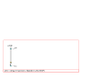
—continues

Figure 6: 1d n-templates, indexed $k$-1 to 0 from left to right, as defined in DDLab for odd and even $k$[27, EDD:10.1.2]. Even-$k$ n-templates are asymmetric, skewed to the right. However, they still support iso-rules as shown in figure 1 where the symmetry is preserved by shifting successive time-steps by $1/2$ cell-space.

(a)$k$=3

(b)$k$=4t

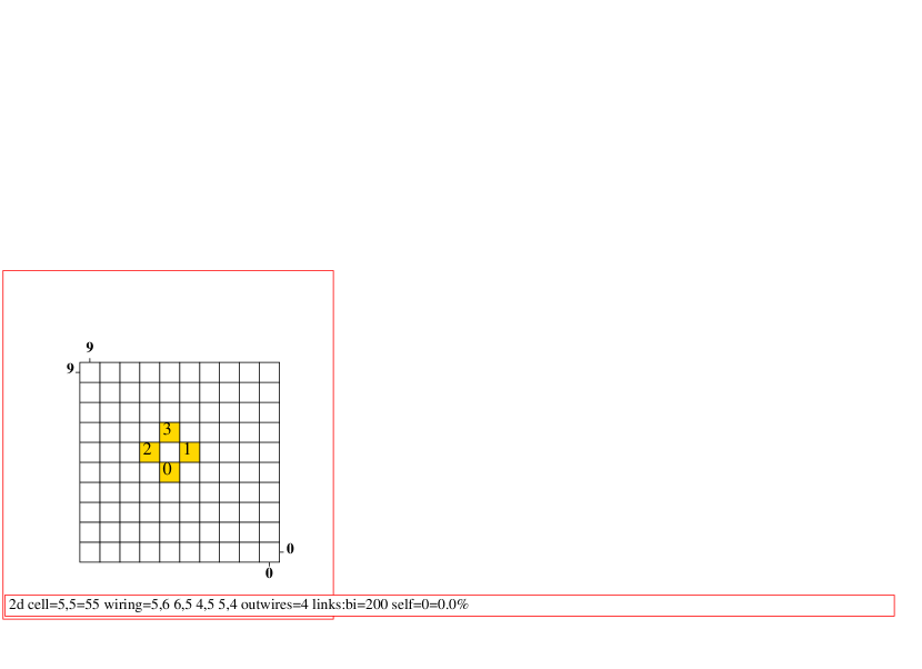
(c)$k$=4s

(d)$k$=5

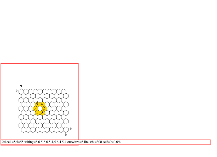
(e)$k$=6

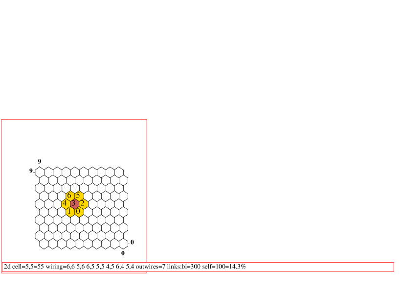
(f)$k$=7

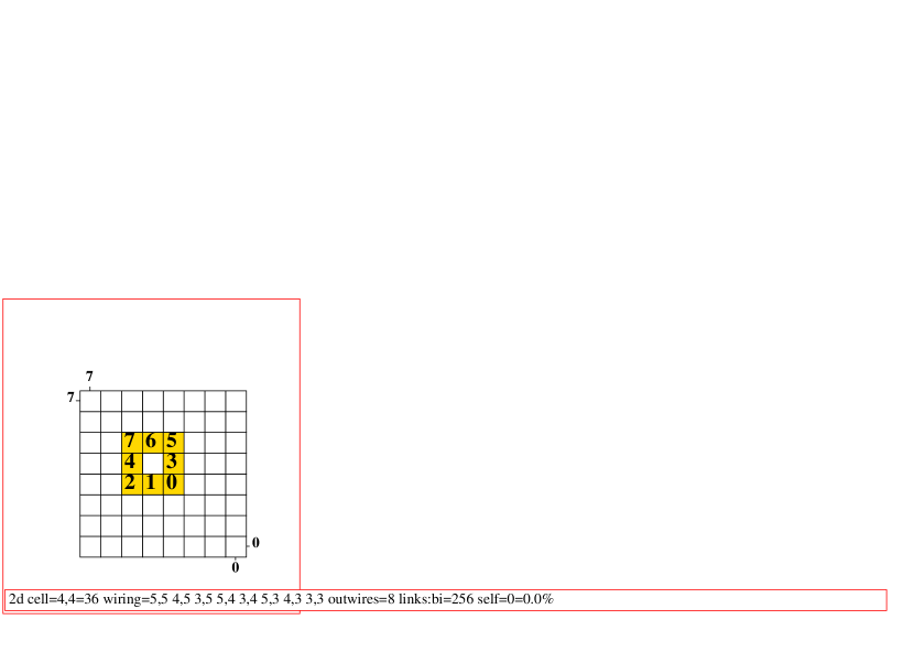
(h)$k$=8

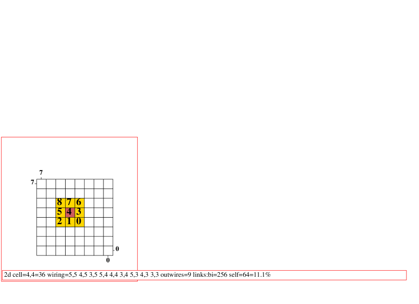
(i)$k$=9

Figure 7: 2D n-templates ($k$=3 to 9) as defined and indexed in DDLab[27, EDD:10], hexagonal or square. $k$=4 n-templates can be either. To achieve periodic boundary conditions hexagonal n-templates require even lattice dimensions. The target cell is central even if not part of the n-template. For 3-value CA, glider rules are readily found for these n-templates as in figure 5.

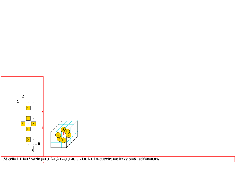
(a)$k$=6

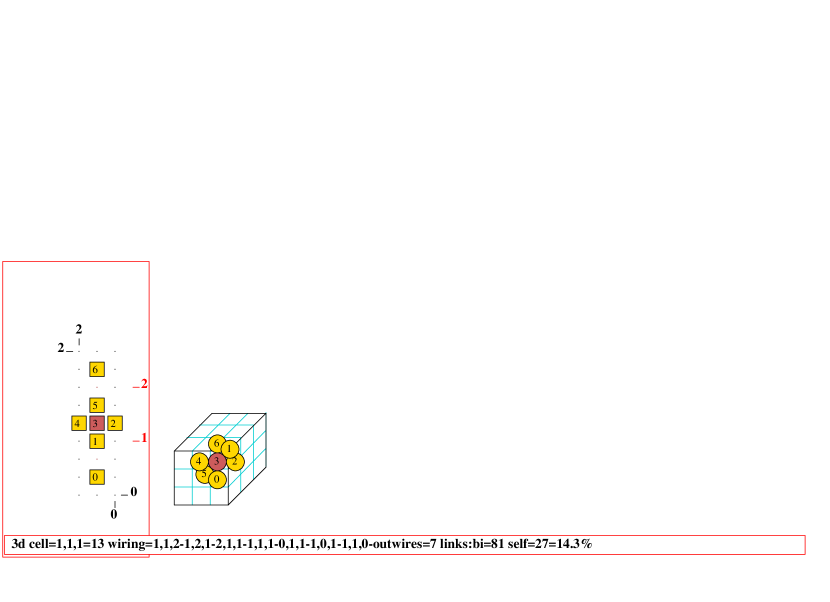
(b)$k$=7

Figure 8: 3d n-templates ($k$=6 or 7) as defined and indexed in DDLab[27, EDD:10]. The target cell is central even if not part of the n-template.

3 rcode, iso-groups and iso-rules

CA rules can be divided and defined according to a number of (possibly overlapping) types[27, EED:13]. These include the full rule-table (rcode), k-totalistic (kcode), t-totalistic (tcode), outer-totalistic, reaction-diffusion, survival/birth, and of course iso-rules.

The most general rule type, rcode, can implement any logic including all the types listed above, and forms the basis for extracting iso-rules. Rcode is a list of the outputs of all $v^{k}$ possible neighborhoods depending only the value-range $v$ and neighborhoods size $k$ giving a rule-space of $v^{v^{k}}$, and is independent of n-template geometry. The list order must be specified, and we follow Wolfram’s classical convention[17, 18]; a descending order of neighborhood binary (or $v$-ary for $v$$>$2) values from left to right which is also the rcode index, as in this example for binary $k$=3 where the decimal equivalent of the rcode string gives the “Elementary Rule” number.

     7    6    5    4    3    2    1    0   - binary value and rcode index
    111  110  101  100  011  010  001  000  - k=3 neighborhoods
     0    0    1    1    1    1    0    0   - output string = rcode 60 in decimal

In DDLab the neighborhoods are displayed vertically for compactness with a $k$ index ($k$-1 to 0, top down), making a so called “neighborhood matrix”, shown here for binary $k$=3, and for $k$=5 where rcode is better expressed in hexadecimal rather than decimal,

rule index - 7......0                   31...... ........ ........ .......0
             :      :                   :                                 :
         2 - 11110000               4 - 11111111 11111111 00000000 00000000
 k-index 1 - 11001100               3 - 11111111 00000000 11111111 00000000
         0 - 10101010       k-index 2 - 11110000 11110000 11110000 11110000
             --------               1 - 11001100 11001100 11001100 11001100
 rcode 193 - 11000001               0 - 10101010 10101010 10101010 10101010
                                        -------- -------- -------- --------
               rcode (dec) 4276676736 - 11111110 11101000 11101000 10000000
                     (hex) fee8e880 (majority rule)

As a reference, the neighborhood matrix is displayed graphically prior to selecting, editing and transforming the rcode. The same matrix principles apply for any values of $v$ and $k$, as in the examples in figure 9.

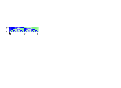
(a) $v2k5$, $2^{5}$=32, complete matrix

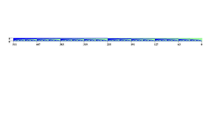
(b) $v2k9$, $2^{9}$=512, complete matrix

(c) $v3k7$, $3^{7}$=2187, left part only

(d) $v5k5$, $5^{5}$=3125, left part only

Figure 9: Examples of various $v$,$k$ matrices showing rcode size.

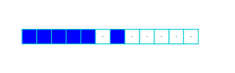
(a) $v2k5$ rcode(32), 2d square iso-rule(12)

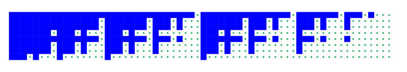
(b) $v2k9$ rcode(512), 2d square iso-rule(102)

(c) $v3k7$ rcode(2187), 2d hex iso-rule(276)

(d) $v5k5$ rcode(3225), 2d square iso-rule(600)

Figure 10: Examples of majority (voting) rules[27, EDD:16.7] for $v$,$k$ in figure 9 presented as bit/value strings (and sizes) as rcode, and transformed to 2d iso-rules. Only binary majority rcode with odd $k$ is isotropic by default when initially selected.

The examples in figure 10 show majority (voting) rcode[27, EDD:16.7] selected in DDLab, where the majority value in each neighborhood becomes its output. In case of a tie, for $v$=2 the central cell wins — the rcode is isotropic by default. For $v$$>$2, or an empty central cell, one of the majority values is picked at random — probably not isotropic. However, the transformation to an iso-rule also induces isotropy in the original rcode. The iso-rule string is much shorter than the rcode-string as can be seen in table 1. Graphical string presentations can be rescaled, adjusted between single or multiple rows, and allow various functions and manipulations with the mouse and keyboard [27, EDD:16.4].

An rcode is transformed to the iso-rule and its graphical string with a keypress [27, EDD:16.10.4] and further options will show iso-groups graphically with accompanying details (figure 11) or the the complete graphic of the iso-rule prototype neighborhoods (figure 12) in a separate window.

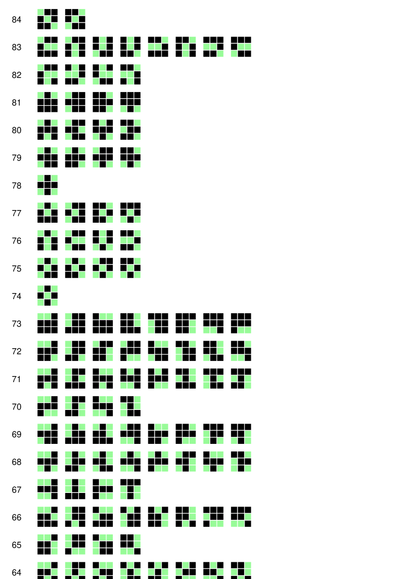
(a) 3 successive $v2k9$ 2d square (Moore) iso-groups for iso-indeces as shown (max=101)

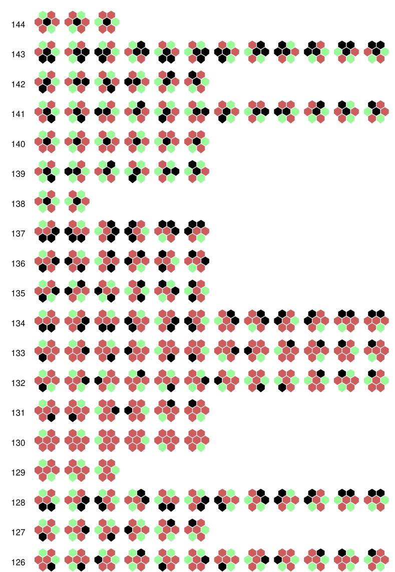
(b) 3 successive $v3k7$ 2d hex iso-groups for iso-indeces as shown (max=275)

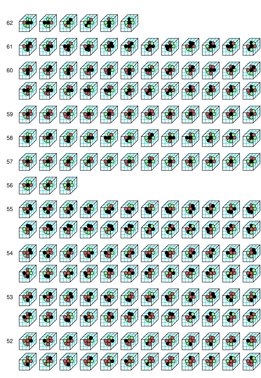
(c) 3 successive $v3k7$ 3d iso-groups for iso-indeces as shown (max=171)

Figure 11: Examples of 3 successive iso-groups shown graphically; their sizes depend on internal symmetries. (a) $v2k9$ has 102 iso-groups, (b) and (c) are both $v2k7$ but (b) is 2d hex with 276 iso-groups, and (c) is 3d with 172 iso-groups.

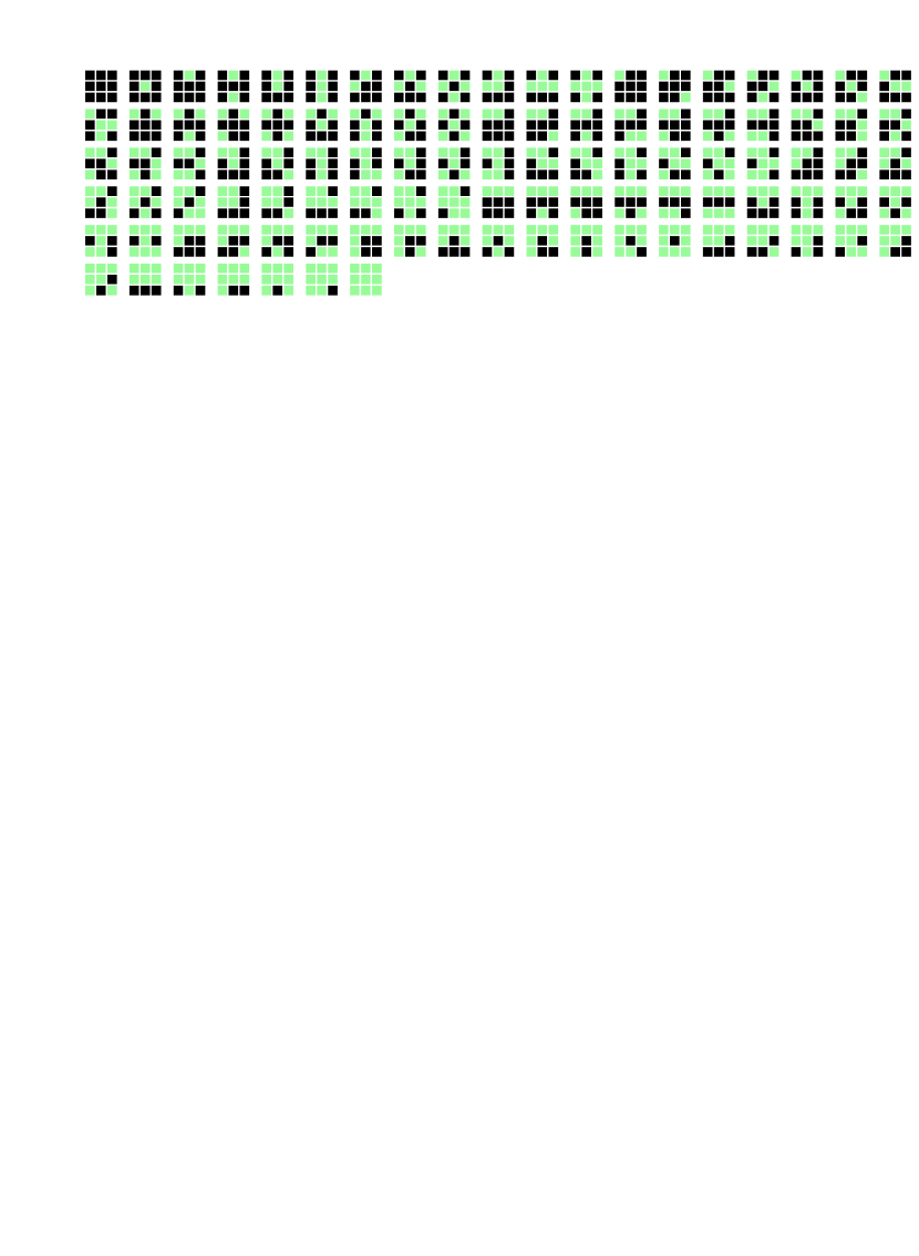
(a) 102 $v2k9$ 2d square (Moore) neighborhood iso-group prototypes

(b) 276 $v3k7$ 2d hex neighborhood iso-group prototypes

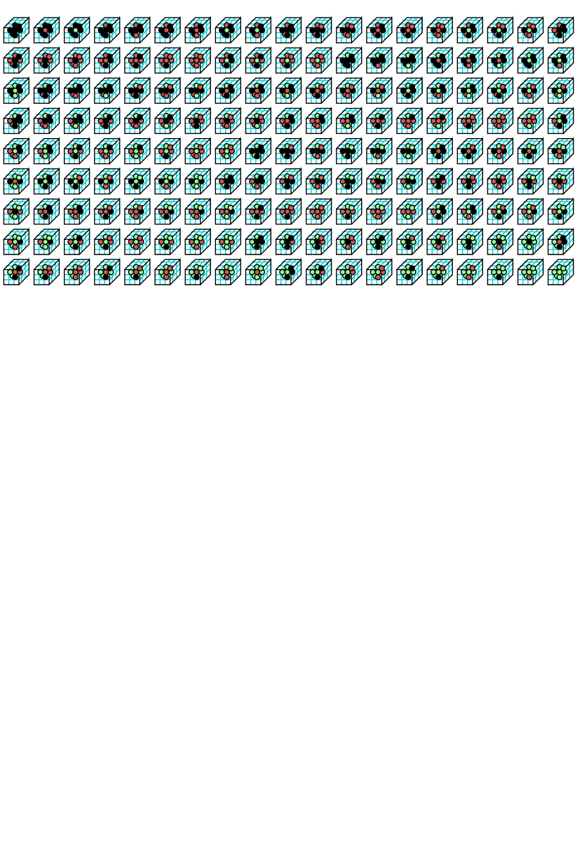
(c) 172 $v3k7$ 3d neighborhood iso-group prototypes

Figure 12: Examples of the complete set of iso-rule n-template prototypes shown graphically in descending order of their decimal equivalents from the top-left. (a) $v2k9$ has 102 prototypes, (b) and (c) are both $v2k7$ but (b) is 2d hex with 276 prototypes, and (c) is 3d with 172 prototypes.

3.1 iso-rule advantages

The iso-rule is arguably an improvement on previous isotropic CA notations, for example by Sapin[14, 15] and Hensel, because the iso-rule is a simple lookup-table in a conventional order and is general, applying to a range of n-template sizes $k$ in 1d, square or hex 2d, and 3d, and extending beyond binary to a range of values $v$. The iso-rule can be computed down by reducing a full CA lookup-table or up by enhancing iso-subsets — totalistic, reaction-diffusion and survival/birth — so provides an intermediate granularity for mutation, bias, manipulation, or in a search by genetic algorithm[14]; isotropy is conserved whatever changes are made to an iso-rule.

In DDLab, the iso-rule provides the basis for input-frequency/entropy, filtering and mutation in the same way as conventional full or totalistic CA lookup-tables: rcode, tcode or kcode. For glider/eater/glider-gun iso-rules, the input-frequency histogram (IFH) identifies both the critical and neutral iso-groups underlying dynamics, and provides methods to explore rule-space that is genetically close to significant iso-rules — the IFH mutation/filter game[27, EDD:16.10.8]. The methods for automatically classifying and examining rule-space based on input-entropy variability[21, 22, 8] can be applied to iso-rules. These ideas are developed further in the paper.

3.2 iso-rule sizes

The sizes of the iso-rule tables for the n-templates in figures 6, 7 and 8 depend on $v$, $k$, and the internal symmetries of the n-template so are difficult to calculate analytically. The tables below give iso-group sizes computed algorithmically in DDLab.

                         1d-k         2   3    4    5    6     7    8    9   10         -----------------------------------------    2 |  3   6   10   20   36    72  136  272  528    3 |  6  18   45  135  378  1134 3321 9963 |  4 | 10  40  136  544 2080  8320 v  5 | 15  75  325 1625 7875 |  6 | 21 126  666 3996    7 | 28 196 1255 8575    8 | 36 288 2080              2d hex-k                      2d square-k                3d-k          3    4    6    7              4    5    8    9              6    7         -----------------             -----------------             -------    2 |   4    8   13   26        2 |   6   12   51  102     |  2 |  10   20    3 |  10   30   92  276        3 |  21   63  954 2862     v  3 |  57  171 |  4 |  20   80  430 1720     |  4 |  55  220               |  4 | 240  960 v  5 |  35  175 1505          v  5 | 120  600                  5 | 800 |  6 |  56  336               |  6 | 231 1386    7 |  74  588                  7 | 406    8 | 120  960                  8 | 666

Table 1: Sizes of iso-rule lookup-tables (number of iso-groups) for 1d, 2d hex, 2d square and 3d n-templates in figures 6, 7, and 8, for $vk$ within non-extended limits[27, EDD:7.1.1] in DDLab.

4 iso-subsets expressed as iso-rules

Significant CA iso-subsets, rule types that are isotropic by default, include k-totalistic (kcode), t-totalistic (tcode), outer totalistic, reaction/diffusion, and survival/birth rules. These iso-subsets have their specific concise definitions and rule-spaces which allow interesting coarse-grained mutations. However, by transforming the iso-subsets to equivalent iso-rules, finer-grained mutations become possible in a search for a wider range of significant rule families. Below, we define these iso-subsets and their rule-spaces.

4.1 k-totalistic rules (kcode)

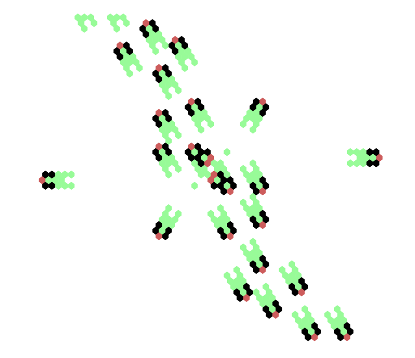
(a) hex 2d glider-gun

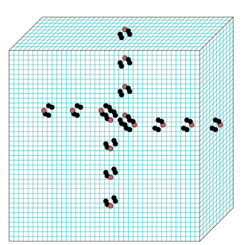
(b) 3d glider-gun

Figure 13: Beehive rule glider-guns $v3k6$ for (a) hex 2d shooting gliders in 6 directions, and (b) 3d 40$\times$10$\times$40 shooting gliders in 4 directions. The 3d glider-gun emerges spontaneously, but localised structures (such as eaters) are absent.

Kcode rules are defined by a list of the outputs for all possible combinations of value-frequencies in the neighborhood. Each combination is represented by a string of length $v$, shown vertically from $v$-1 down in this example for the $v3k6$ Beehive rule[22, 1, 23]) with frequencies of values 2 to 0, which must add up to $k$, so the last row of frequencies is redundant and could be omitted.

               27..........................0 <--k=6 kcode index                 |                          |            > 2: 6554443333222221111110000000  < frequency strings       6    0 v=3 values > 1: 0102103210432105432106543210  < of 2s, 1s, 0s,     from 0 to 0            > 0: 0010120123012340123450123456  < shown vertically        0    6                 ||||||||||||||||||||||||||||                 0022000220022001122200021210 <--kcode, outputs [0,1,2]                                    beehive rule (hex) 0a0282816a0264

In the spirit of Wolfram’s convention[17], the ordering of the combinations depend on their $v$-ary value, with the higher kcode index on the left. Kcode rules are independent of the n-template; they are isotropic because the positions of values in are irrelevant.

In the example above for $v3k6$, outputs [0,1,2] are listed in reverse order of the kcode index, and can be expressed in decimal (if applicable) or in hexadecimal. DDLab automatically transforms kcode into its equivalent rcode, which can then be transformed to isotropic rcode and the iso-rule according to the n-template. The 2d $v3k6$ Beehive rule on a hex lattice also works on a 3d lattice, and both support a glider-gun (figure 13). The 2d ad 3d iso-rules are different, with lengths 92 an 57 respectively as shown below as a table and in hex,

(92) 00220200000102000222020022222222222122220222212102222221022000220222022222212000022212022010 (hex) 0a 20 01 20 2a 20 aa aa a9 aa 2a 99 2a a9 28 0a 2a 2a a9 80 2a 62 84 (57) 202200001120002222222221210202200022220222122120021022010 (hex) 02 28 01 60 2a aa a6 48 a0 2a 8a 9a 60 92 84

The size of a kcode-table, $S_{k}=(v+k-1)!/(k!\times(v-1)!)$, and increases more slowly than iso-rule size for larger $vk$ as in the table below,

                     -- k --         2   3   4   5    6    7    8     9    10         ----------------------------------------    2 |  3   4   5   6    7    8    9    10    11    3 |  6  10  15  21   28   36   45    55    66 |  4 | 10  20  35  56   84  120  165   220   286 v  5 | 15  35  70 126  210  330  495   715  1001 |  6 | 21  56 126 252  462  792 1287  2002  3003    7 | 28  84 210 462  924 1716 3003  5005  8008    8 | 36 120 330 792 1716 3432 6435 11440 19448

Kcode where $v$=3 can be expressed as an $ij$-matrix based on the frequency of 2s and 1s (0s are given by $k-(i+j)$ so are not required). Such rules can be reinterpreted as conceptual discrete models of reaction-diffusion systems with inhibitor and activator reagents[1, 2]. Figure 2 gives examples.

$\begin{array}[]{ll|llllllll}&&&&&&j&&&\cr&&0&1&2&3&4&5&6\cr\hline\cr&0&0&1&\color[rgb]{0,0,1}2&\color[rgb]{1,0,0}1&\color[rgb]{1,0,0}2&\color[rgb]{1,0,0}0&\color[rgb]{1,0,0}0\cr&1&0&2&\color[rgb]{0,0,1}2&2&\color[rgb]{1,0,0}1&\color[rgb]{1,0,0}1&\cr&2&0&\color[rgb]{1,0,0}0&\color[rgb]{0,0,1}2&2&\color[rgb]{1,0,0}0&&\cr i&3&0&2&\color[rgb]{0,0,1}2&\color[rgb]{1,0,0}0&&&\cr&4&\color[rgb]{1,0,0}0&\color[rgb]{0,0,1}0&\color[rgb]{0,0,1}2&&&&\cr&5&\color[rgb]{0,0,1}2&\color[rgb]{0,0,1}0&&&&&\cr&6&0&&&&&&\cr\end{array}$
Beehive rule

$\begin{array}[]{cc|cccccccc}&&&&&&j&&&\cr&&0&1&2&3&4&5&6&7\cr\hline\cr&0&0&1&2&\color[rgb]{1,0,0}1&\color[rgb]{0,0,1}2&\color[rgb]{0,0,1}2&\color[rgb]{1,0,0}2&\color[rgb]{1,0,0}2\cr&1&0&2&2&\color[rgb]{1,0,0}1&\color[rgb]{1,0,0}2&\color[rgb]{1,0,0}2&\color[rgb]{1,0,0}2&\cr&2&0&0&2&\color[rgb]{0,0,1}1&\color[rgb]{1,0,0}2&\color[rgb]{1,0,0}2&&\cr i&3&0&2&2&1&\color[rgb]{0,0,1}2&&&\cr&4&0&0&2&1&&&&\cr&5&0&0&\color[rgb]{0,0,1}2&&&&&\cr&6&0&0&&&&&&\cr&7&\color[rgb]{0,0,1}0&&&&&&&\cr\end{array}$ Spiral rule

Table 2: The $ij$-matrices of (left) the $v3k6$ Beehive rule [22, 1, 23] and (right) the $v3k7$ Spiral rule [24, 2, 25], on 2d hex lattices. The output can be read off from the frequency of 2s (rows $i$) and 1s (columns $j$). Previous studies (as cited above) have shown that a significant proportion of outputs are quasi-neutral — wildcards — with little impact on dynamics. These are shown in color: red for strong wildcards, blue for weak wildcards.

4.2 t-totalistic rules (tcode)

Tcode rules are defined by a list of outputs for each possible total, the sum of values in the neighborhood, and are useful for setting threshold functions. Tcode is a subset of kcode because each total can include several kcode combinations of value-frequencies, so tcode is also isotropic, but more directly because any n-template’s rotation/reflection must give the same total. The size of a tcode-table $S_{t}=k(v-1)+1$.

To set tcode each total is set out in reverse value order, $S_{t}$-1 to 0, and is assigned an output [0,1,$\dots$,$v$-1], which is the tcode value-string. Here is an example for the $v5k5$ majority rule,

  20...................0 - all possible totals    |                   |    444433332222111100000 - tcode, outputs [0,1,2,3,4]                            (hex) 49236da491248000

Tcode may be expressed in decimal (if applicable) or in hexadecimal. DDLab automatically transforms tcode into its equivalent rcode, which can then be transformed to isotropic rcode and the iso-rule according to the n-template. For the majority rule (above) the rule tables for rcode (size 3225), and the iso-rule (size 600) for a 2d square n-template, are shown graphically in figure 10(d).

For binary ($v$=2), tcode depends on just the sum of 1s the neighborhood so tcode and kcode are identical, $S_{t}$=$S_{k}$, but for $v$$\geq$=3 $S_{t}$ becomes progressively smaller than $S_{k}$. Here is an example of binary tcode for the $v2k5$ majority rule, its rcode, and iso-rule on a 2d square n-template.

   5 4 3 2 1 0 - all possible totals    - - - - - -    1 1 1 0 0 0 - output = tcode = kcode, 56 in dec, 38 in hex,                  rcode = 11101000100000011000000100010110                  iso-table(12)=111110100000 (hex)0f a0

4.3 outer-totalistic kcode or tcode

Outer-totalistic CA require $v$ rules, one for each possible value of the center cell, so the size of the total string $S_{o}$ is $v$$\times$$S_{k}$ for kcode, or $v$$\times$$S_{t}$ for tcode. The method in DDLab works with any $vk$, but makes most sense if the central cell is empty in the n-template.

Binary ($v$=2) Life-like 2d CA can be defined by two $k$=8 tcode rules, with a total table size $S_{o}$=18, whereas the equivalent $S_{i}$=102 and $S_{r}$=512. For the game-of-Life two $v2k8$ tcodes can be set “by hand”[27, EDD:13.7] for the central cell of 0 and 1 as follows,

0: 000001000 - birth: exactly 3 live neighbors

1: 000001100 - survival: 2 or 3 live neighbors

$k$8 n-template

However, DDLab has automatic methods for setting the game-of-Life and other survival/birth rules (section 4.5) as both outer-kcode[27, EDD:14.2.2] and as full rcode rule-tables[27, EDD:16.10.7] which limits the $vk$ range but allows reassigning as equivalent iso-rules.

4.4 reaction-diffusion rules

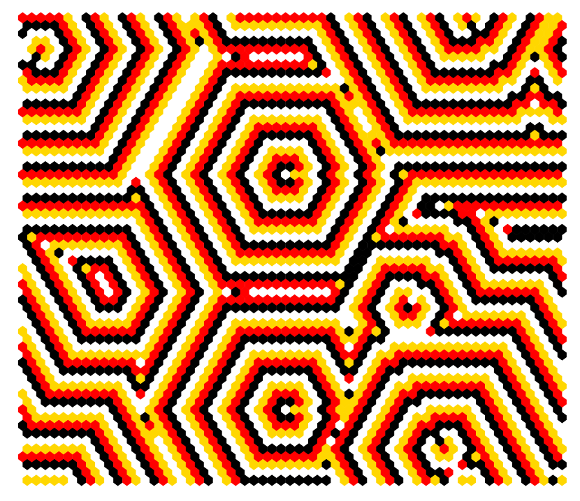
(a) unfiltered

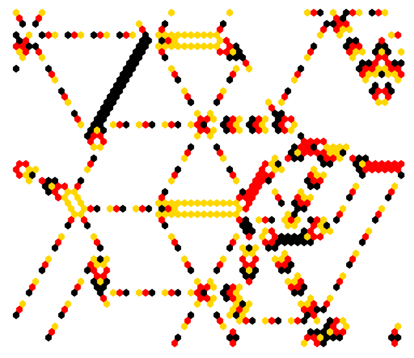
(b) filtered

Figure 14: Snapshots of a hex 2d reaction-diffusion CA $v4k7$, with the iso-rule (size 1720) shown below. The threshold interval was set 1 to 4. The initial state 60$\times$60 has a low density (0.01) of non-zero cells. (a) the emergent pattern, and (b) the pattern with the 3 most frequent iso-groups filtered, showing structures that resemble glider-guns.

Reaction-diffusion or excitable media dynamics [13], can be generated with a type of CA with 3 cell qualities: resting, excited, and refractory (or substrate, activator, and inhibitor). The rules are isotropic by default because they are basically totalistic, depending on just totals of values in the neighborhood. There is usually one resting type, one excited type, and one or more refractory types. In DDLab these correspond to the values $v$=0, $v$=1, and $v$$\geq$2, which cycle between each other. A resting cell (0) remains as is until the number of excited cells in its neighborhood falls within the threshold interval $t$, whereupon it becomes excited (1). An excited cell (1) changes to the first refractory value (2) at the next time-step, then to the next refractory value (3) and so on, and the final ($v$-1) refractory value changes back to resting (0), completing the following clockwise cycle,

 resting(0)--->if within t threshold interval           \               \            \              (1) excited             \               \             (v-1)<----(3)<--(2) refractory

The variables required to define a reaction-diffusion rule are $vk$ and the threshold interval within $k$. The number of refractory values is $v$-2. In DDLab, reaction-diffusion[27, EDD:13.8] can be set as rcode which allows transformation to an iso-rule, or as outer-kcode which allows a greater range of $vk$.

The resulting dynamics, in 2d or 3d, can produce waves, spirals and related patterns that can resemble the Belousov-Zhabotinsky reaction in a non-linear chemical medium and other types of excitable media. Filtering the wave-like patterns by descending frequency of iso-groups can reveal dynamics reminiscent of glider-guns (figure 14). The filtering method[27, 32.11.5] is based on the input-frequency histogram described in later sections.

As well as the threshold interval, the dynamics are sensitive to the initial state and its density of non-resting types (non-zero values)[27, 21.3] — usually low for best spiral-wave results.

4.5 survival/birth rules

A survival/birth rule, including the game-of-Life, can be set in DDLab[27, EDD:16.10.7]. The rule is turned into rcode automatically and can then be transformed into an iso-rule (figure 15). The rcode of the iso-rule can be transformed for a negative universe as in figure 16 by complementing both neighbourhoods and outputs[27, 18.5.2].

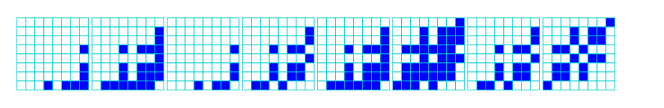
Figure 15: Conway’s game-of-Life (s23/b3) shown as a 512 bit rcode in 8 rows. The diagonal symmetry in each 8x8 block is a necessary (but insufficient) indication of isotropy but a useful visual clue for the general case of isotropic rcode for a binary $v2k9$ 2d CA with a Moore neighborhood. Below the rcode is the 102 bit iso-rule — (hex) 00 00 00 00 00 60 03 1c 61 c6 7f 86 a0.

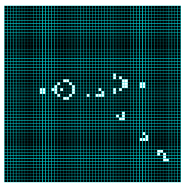
Figure 16: The negative game-of-Life with a negative Gosper glider-gun. The iso-rule is
(hex) 3e a7 a2 46 5b e2 df 7d f7 df ff ff ff. A negative[27, EDD:18.5.2] iso-rule gives equivalent dynamics given a complementary initial state, which would reduce the effective size of iso-rule-space.

DDLab defines the classical game-of-Life as (s23/b3) following a common shorthand for survival/birth[16], though this is often reversed to birth/survival (b3/s23)[4]. A cell is either alive (1) or dead (0). The first part of (s23/b3) defines the survival of a cell requiring 2 or 3 live neighbors, the second defines birth, requiring 3 live neighbors, otherwise the cell is dead by overcrowding or exposure. Any other survival/birth settings can be selected in this notation, for example (s1357/b1357) for Fredkin’s replicator (figure 17).

Figure 17: Fredkin’s replicator. An initial pattern (the eye) re-emerges from apparent disorder as partial or complete multiple copies (time-steps 1, 17, 25, 33).

The survival/birth option is available for $v$$\geq$2, and any $k$$\geq$5 as well as the $k$=9 neighborhood, for 1d and 3d as well as 2d. For $v$$\geq$3 any value $v$$>$0 is considered alive and the algorithm in DDLab generates an equivalent rcode/iso-code giving dynamics similar to binary, but including $v$ colors as in figure 18.

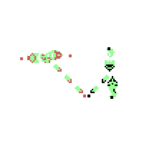
Figure 18: The game-of-Life (s23/b3) applied to a $v$=3 CA. The algorithm in DDLab generates an equivalent rcode and iso-rule (size=2862). The dynamics is the same as binary Life but with 2 colors + background. This example shows two different color Gosper glider-guns, and added green dynamic trails.

5 rule-table size summary

The sizes of rule-tables, or the amount of information required, $S$, to define different rule or logic types, with a rule-space of $v^{S}$ are summarised below,

• $S_{r}=v^{k}$

• $S_{i}$: according to $vk$ and n-template as in table 1

• $S_{k}=(v+k-1)!/(k!\times(v-1)!)$

• $S_{t}=k(v-1)+1$

• $S_{ok}$ = $v$$\times$$S_{k}$

• $S_{ot}$ = $v$$\times$$S_{t}$

• $S_{RD}$ $<$ $S_{ot}$, ($v$, $k$ and threshold interval)

• $S_{SB}$ $<$ $S_{ot}$, (survival and birth totals)

In general, $S_{r}$$>$$S_{i}$$>$$S_{k}$$>$$S_{t}$. $S_{RD}$ $<$ $S_{ot}$ and $S_{SB}$ $<$ $S_{ot}$ because both reaction-diffusion and survival/birth logic can be set within t-outer-totalistic rules.

6 input-frequency histogram (IFH)

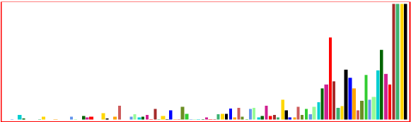
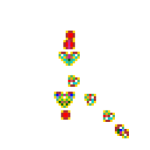
i Life

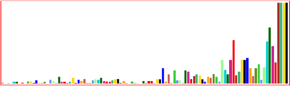
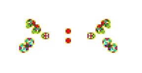
Eppstein

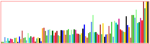
Eppstein random initial state

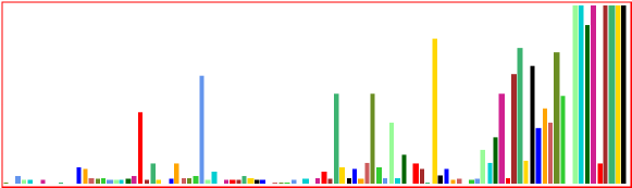
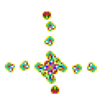
SapinR

Figure 19: The input-frequency histograms (actual plots) in a moving window of 100 time-steps, for the glider-guns of the following rules: Life, Eppstein (shown also from a random initial state), and SapinR, all from figure 4(a). Pattern snapshots are colored to match histogram colors. Note that apart from its glider-gun, the Eppstein rule is chaotic.

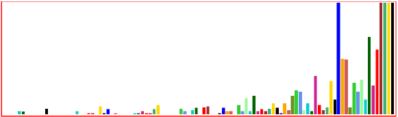
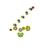
Variant

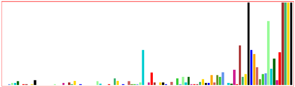
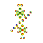
Precursor

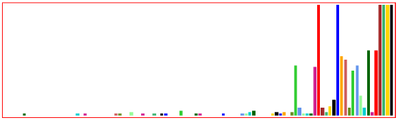
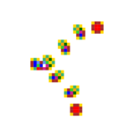
Sayab

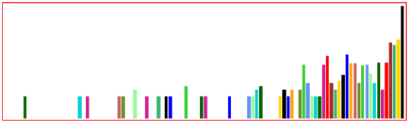
i left: the same Sayab histogram as above but on the alternative log₂ plot

Figure 20: The IFH (actual plots) in a moving window of 100 time-steps, for the glider-guns of the following rules: Variant, Precursor, and Sayab with an alternative log₂ plot, all from figure 4(b). Pattern snapshots are colored to match IFH colors.

While iterating CA space-time patterns, DDLab is able to keep track of the frequency of rule-table lookups in a moving window of time-steps by means of a dynamic “input-frequency” histogram (IFH)[27, EDD:31.5]. This applies to any rule type. For complex rules the IFH reveals the key inputs (neighborhoods or iso-groups) that maintain gliders and glider-guns, as well as those that are rarely or never visited.

Figures 19 and 20 show IFH examples for iso-rules generated by the glider-guns shown alongside. The moving window can be any size but here it is set to 100 time-steps to allow the IFH to stabilise. The input-frequency is the fraction of each iso-group in this window, and is represented by bar height. The order of bars follows the iso-rule index, from all 1’s (left) to all 0’s (right), and a missing bar denotes iso-groups that have not been visited. The bar height can be represented in two ways: either the actual frequency but (possibly) amplified to show up small bars of rarely visited iso-groups while the most visited are subject to a maximum cut-off, or alternatively as log₂ frequency to clearly show all bars but still distinguishes between rare and frequent. There are also two types of space-time pattern presentation: cells colored according to their actual values, or colored according to the IFH bar responsible for a given cell, as in these figures. These alternatives are toggled on-the-fly.

Figures 19 and 20 show histograms for the the binary $v2k9$ glider-gun iso-rules in figure 4 on a 3$\times$3 Moore neighborhood with 102 iso-groups. The Sayab histogram is shown both according to actual frequency, and according to log₂ frequency which will be employed in further examples.

DDLab applies the IFH for a number of supplementary functions. Filtering permits cross referencing a particular iso-group index with its occurrence in space-time pattern, as well as revealing structures within a repetitive background. The consequences of mutations can be monitored by flipping (and restoring) the output of random or selected iso-groups to a different value. The Shannon entropy of the histogram and its variability are applied to automatically categorise rule-space between order, complexity and chaos. These functions are discussed below.

7 filtering

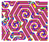
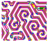
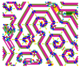
xf1-3xxx

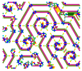
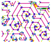
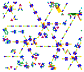
xf3-6xxx

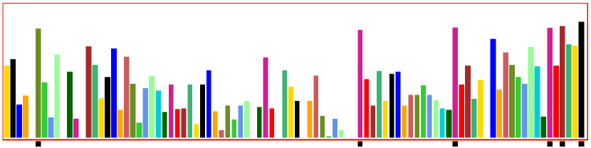
Figure 21: The $v3k6$ emergent spirals rule with a log₂ iso-rule IFH size 92 in a moving window of 100 time-steps. Space-time pattern cells are colored according to the histogram bar responsible for that cell. For the same time-step, 6 stages of filtering f1 to f6 (high to low frequency) are marked by a black block below the relevant bar, and shown as a filtered snapshots. Filtering f1 makes no difference to its appearance because white cells are the most frequent, represented by the rightmost black bar. In the dynamics of this rule gliders first emerge and gradually self-organise into stable spirals.

The IFH allows the progressive filtering/unfiltering[27, EDD:32.11.5] of space-time patterns on-the-fly by keyhits as space-time patterns iterate. This applies for any rule type according to frequency given by the height of histogram bars. Progressive filtering proceeds from high to low frequency, unfiltering from low to high. For each frequency filtered/unfiltered, a black block appears/disappears at the base of the relevant bar, and the corresponding cell disappears/reappears in the space-time pattern, whether colored by histogram colors as in figure 21, or by value as in figure 14. Keyhits can remove the entire filter scheme or reverse (antifilter) the scheme for added flexibility. Bars can also be targeted to filter/unfilter[27, EDD:32.16.7], and mutated/restored described in section 8 below.

When pattern colors correspond to IFH colors, filtering allows cross referencing a particular iso-group index with its occurrence in the space-time pattern, so helps to reveal how complex structures, gliders, eaters and glider-guns are built and their sensitivity to mutation. The IFH in figure 21 is set for a moving window of 100 time-steps to allow the bars to stabilise. However, if the pattern itself has largely stabilised and the moving window size is reduced (minimum one time-step), then the few structures that remain dynamic can be picked out in the IFH by the bars that continue to oscillate.

To determine the iso-groups responsible for any particular structure, say the glider in the game-of-Life, an isolated glider is run to generate its iso-rule IFH, which if fully filtered will provide the complete list of the responsible iso-groups in descending frequency order, as in figure 22.

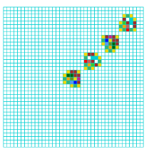
i The 4 phases of the game-of-Life glider, moving North East. far left: colors by value with green dynamic trails. near left: colors corresponding to histogram colors.

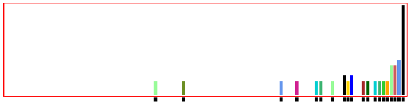
Figure 22: The log₂ iso-rule IFH of the game-of-Life glider in a moving window of 10 time-steps showing the 20 bars (from a maximum of 102) that are responsible for the glider’s existence. When these are filtered as marked by black blocks, the iso-group indices, in descending frequency order (63,56,31,27,22,21,18,15,14,13,10,9,7,6,5,4,3,2,1,0) can be viewed and amended in a separate window.

8 the IFH mutation/filter game

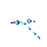
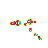
i The game-of-Life glider-gun. far left: colors by value with green dynamic trails. near left: colors corresponding to IFH colors.

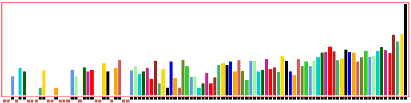
i Blow up of the left lower corner showing indicator blocks: filter (black) and mutation (red).
The iso-rules (hex) are compared below:
00 00 00 00 00 60 03 1c 61 c6 7f 86 a0 ---game-of-Life.
34 e6 e4 64 c0 60 03 1c 61 c6 7f 86 a0 ---after all 17 neutral mutations.

Figure 23: The log₂ iso-rule IFH of the game-of-Life glider-gun/eater. The all active bars were firstly filtered, then all 17 neutral bars were mutated. The glider-gun/eater is preserved, though any other dynamics would be drastically altered.

The IFH allows interactive (or targeted) rule mutations[27, EDD:32.5.4] while watching their effects on space-time patterns, to make/restore single mutations on-the-fly with keyhits, without the need to pause, in a sort of mutation/filter game[27, EDD:16.10.8]. Any number of mutations can be made in sequence, and restored in reverse order to finally return to the start rule. When applied to an iso-rule, mutations conserve isotropy, of course.

The mutation algorithm can operate in conjunction with on-the-fly filtering described in section 7. The keyhit to mutate will preferentially select an unfiltered iso-group bar at random and assign a random value different from the current output. For a binary rule the output is simply flipped. A red block is shown at the base of the bar — beside the black filter block if this is also active. When the latest mutation is restored its red block is removed.

To observe the effects, the appearance of pattern filtering can be toggled off/on with a keyhit while the IFH filtering scheme remains visible. The mutation game can be the most effective if all active bars have been filtered because a mutation to an inactive iso-group will be neutral for self-contained dynamics such as a glider-gun/eater system.

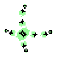
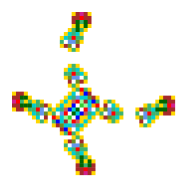
i The SapinR glider-gun. far left: colors by value with green dynamic trails. near left: colors corresponding to IFH colors.

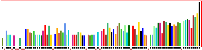
The iso-rules (hex) are compared below:
24 01 13 1a 14 20 50 2c 45 05 48 e0 50 ---SapinR.
1a fe e9 c4 79 87 23 c3 4a 0d 48 e0 50 ---after all 14 neutral mutations.

Figure 24: The log₂ iso-rule IFH of the SapinR rule glider-gun/eaters. All active bars were firstly filtered, then all 14 neutral bars were mutated. The glider-gun/eaters are preserved, though other dynamics would be drastically altered.

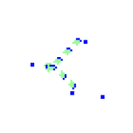
i The Sayab glider-gun. far left: colors by value with green dynamic trails. near left: colors corresponding to IFH colors.

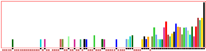
The iso-rules (hex) are compared below:
24 01 13 1a 14 20 50 2c 45 05 48 e0 50 ---Sayab.
1a fe e9 c4 79 87 23 c3 4a 0d 48 e0 50 ---after all 52 neutral mutations.

Figure 25: The log₂ iso-rule IFH of the Sayab rule glider-gun. All active bars were firstly filtered, then all 52 neutral outputs mutated. The glider-guns are preserved, though other dynamics would be drastically altered.

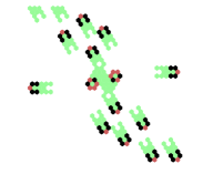
i The Beehive glider-gun with NULL boundary conditions. far left: colors by value with green dynamic trails. near left: colors corresponding to IFH colors.

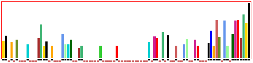
above: the iso-rule IFH representing 92 iso-groups, 40 are active.
The iso-rules (hex) are compared below:
8a 20 01 60 2a 20 aa aa a9 aa 2a 99 2a a9 28 0a 2a 2a 69 80 2a 62 84 --Beehive
86 20 85 a0 1a 10 a4 a4 08 69 98 05 62 a8 20 06 02 26 66 80 0a a2 84 --52 neutral mutations
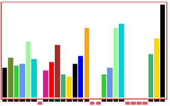
i left: The same Beehive rule glider-gun as a k-totalistic rule IFH representing 28 combinations of totals, The kcodes (hex) are compared below: 0a0682822a1424 ---Beehive
0a0282816a2264 ---after 7 neutral mutations. All one-value mutation were explored in [23].

Figure 26: The $v3k6$ Beehive rule[22] glider-gun showing both its log₂ iso-rule and k-totalistic IFH. Because the Beehive rule does not have eaters to stop gliders, boundary conditions were set to NULL. The IFH were firstly filtered then neutral outputs randomly mutated, with each mutation making one of the two possible changes because $v$=3. The glider-gun is preserved, though other dynamics would drastically be altered.

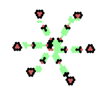
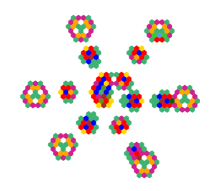
i The Spiral glider-gun. far left: colors by value with green dynamic trails. near left: colors corresponding to histogram colors.

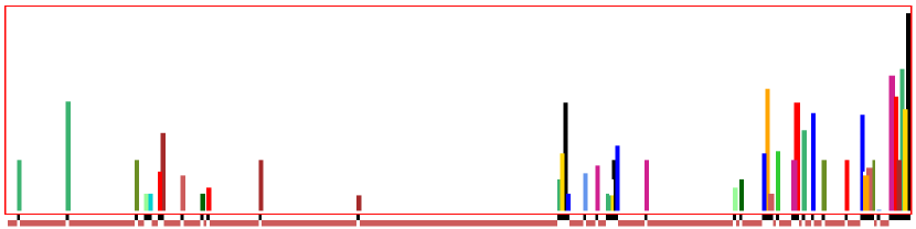
above: the iso-histogram representing 276 iso-groups, 46 are active.
The iso-rules (hex) are compared below:
00 a6 58 a6 66 a6 6a aa a6 a8 02 90 08 96 28 02 92 08 98 a6 69 2a 66 65 9a 69 8a 9a a6 69 a2
66 6a 96 96 6a a9 a9 a6 66 a9 69 08 82 68 28 02 a6 a2 69 a6 66 66 99 a2 62 a6 98 8a 26 08 8a
26 64 9a 40 2a 62 84 --Spiral
98 08 06 21 15 50 94 45 59 50 52 60 51 58 94 49 44 95 25 60 96 84 89 10 44 94 16 00 50 85 19
99 81 00 29 80 54 56 51 08 44 00 08 18 46 10 00 41 46 04 59 09 10 46 04 81 81 00 82 41 04 69
a9 9a a5 00 18 02 84 ---after all 233 neutral mutations.
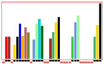
i left: the k-totalistic histogram representing 36 combinations of totals, The kcodes (hex) are compared below: 020609a2982a68aa64 ---Spiral.
410605a01805a845a4 --after 14 neutral mutations.

Figure 27: The Spiral glider-gun showing both its log₂ iso- and k-totalistic histograms. The histograms were firstly filtered then neutral outputs randomly mutated, with each mutation making one of the two possible changes because $v$=3. The glider-gun is preserved, though other dynamics would be altered.

In the examples in figures 23 to 28 the initial state is an isolated glider-gun, in most cases contained by eaters. All active bars are first filtered marking them with black blocks, then mutations are made which automatically and randomly seek out unfiltered inactive iso-groups represented by missing bars, marking them with red blocks. Because these are neutral mutations the relevant glider-gun system must be preserved.

The mutation game is applied to the $v2k9$ rules: game-of-Life, SapinR, Sayab, and also the hex lattice $v3k6$ Beehive rule and $v3k7$ Spiral-rule — both of which feature a 3d glider-gun (figure 13). Sayab, SapinR, the 3d Beehive-rule and the Spiral-rule (both 2d and 3d) are special in the sense that their glider-guns emerge spontaneously from random initial states, whereas glider-guns for other rules covered in this paper need careful construction.

The take-home message from these experiments is the existence of a vast web of connected but diverse iso-rules that support the same glider-gun systems.

Once all gaps have been mutated, further mutations will hit active bars disrupting glider-guns, which can be retrieved with keyhits to unmutate and eventually (or immediately) reinstate the original rule. A keyhit can also reinstate the original glider-gun pattern.

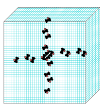
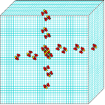
i The Spiral 3d glider-gun. far left: colors by value. near left: colors corresponding to IFH colors.
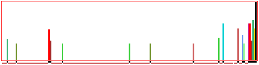
above: the iso-histogram representing 171 iso-groups, 19 are active.
The iso-rules (hex) are compared below:
2a 04 8a 01 22 04 06 56 04 95 a4 96 44 84 82 22 52 25 01 06 25 51 8a 61 64 15 59 56 19 21 06
59 20 a1 60 18 02 45 01 12 00 02 84 --Spiral3d.
04 29 59 98 45 59 59 29 02 6a 69 49 22 59 58 58 04 90 58 50 90 82 61 06 91 0a 22 28 62 4a 69
84 65 26 89 86 51 82 58 8a 90 a2 84 ---after all 152 neutral mutations.

Figure 28: The log₂ iso-rule IFH of the Spiral3d glider-gun with iso-rule size=171 — shorter than Spiral2d size 276. The 3d glider-gun emerges spontaneously, but stable structures (such as eaters) are absent. The IFH were firstly filtered then neutral outputs mutated. The glider-guns are preserved, though other dynamics would be altered.

Mutations to active iso-groups can be done progressively by unfiltering the least active bars, or a specific mutation index can be selected. Any mutation to an active iso-group will change the current space-time dynamics to a greater or lesser extent. If the change is interesting, a new glider or eater, the mutation can be retained. An undesirable change such as excessive disorder can be repaired. Among functions in DDLab that can assist in these experiments are on-the-fly keyhits for a random pattern, and for a random central block[27, EDD:32.8.1], respecting densities previously specified. Space-time patterns can be paused at any time to edit or save the current state or iso-rule and access other functions[27, EDD:32.16].

Exploring state-space genetically close to significant k-totalistic rules was done for the Beehive-rule[21] and the Spiral-rule[24], looking at all possible single k-totalistic mutants[23, 25] and some significant alternative behaviours were discovered. A finer grained search based on iso-rules is now possible.

9 input-entropy and min-max variability

————–1$\longrightarrow$——————————time-steps $\longrightarrow$——————————250
entropy1 xentropy entropy0 \begin{overpic}[height=173.44534pt,width=359.90538pt]{pdf-figs/Life250-entropy} \put(55.0,19.5){\large----------} \put(50.0,12.0){\large----------} \put(57.0,17.0){\large$\uparrow$} \put(57.0,14.5){\large$\downarrow$} \put(55.0,21.5){min-max} \put(7.0,30.0){\large$\leftarrow$} \put(12.0,30.0){ignore initial time-steps} \end{overpic}

Figure 29: Top: 250 time-steps of the game-of-Life from a random 40$\times$40 initial state with a density of 30% shown as a type of axonometric projection where time-steps progress from left to right. Colors follow the iso-rule IFH. Above: The entropy plot generated simultaneously: x-axis time-steps 1 to 250, y-axis normalised Shannon entropy $H_{N}$ from 0 to 1. The min-max entropy is the greatest upslope after a short initial run, 22 time-steps for the scatter-plots in figure 30.

The entropy of the iso-rule IFH, the input-entropy, can be measured and plotted over time. The average entropy and its variability over a window of time-steps indicates the quality — ordered/complex/chaotic — of the dynamics, very roughly as follows,

	order	complexity	chaos
mean-entropy	low	medium	high
entropy-variability	low	high	low

Both the mean-entropy and entropy-variability are measured from a run of time-steps starting from a random (but possible biased) initial state, discounting a short initial run to allow the dynamics to settle into its typical behaviour.

The Shannon entropy of the IFH measures its heterogeneity[21]. The input-entropy[27, EDD:33.1] $H$, at time-step $t$, for one time-step ($w$=1), is given by $H^{t}=-\sum_{i=0}^{S-1}\left({Q_{i}^{t}}/{n}\times log_{2}\left({Q_{i}^{t}}/{n}\right)\right)$, where $Q_{i}^{t}$ is the actual height of bar $i$ (input-frequency) at time-step $t$. $S$ is the number of bars (rule-table size) and $n$ is the CA lattice size. The normalised input-entropy $H_{N}$ is a value between 0 and 1, $H_{N}=H^{t}/log_{2}n$ used in the graphic display as in figure 29 and is usually averaged over a small moving window of time-steps (say $w$=10) to smooth an otherwise jagged plot.

The mean entropy is the average $H_{N}$ over a longer run of time-steps. The entropy-variability known as min-max is the maximum up-slope found in a run of time-steps — the rise in entropy following a lower value.

High entropy variability can be produced by glider dynamics, because collisions create local chaos raising the entropy, from which gliders re-emerge lowering entropy. The basic argument is that if the entropy continues to vary sufficiently in typical dynamics, moving both up and down, then some kind of large scale structural interactions are unfolding. As well as glider dynamics, this might include competing zones of ordered domains, of order and chaos, of domains of competing chaos, or some combination of the above.

Low entropy variability is a consequence of both steady chaos or steady order especially when patterns stabilise or freeze. However, the mean entropy for chaos is high, for order low. In this way the quality of dynamics can be distinguished.

10 automatically classifying rule-space

The two measures, mean entropy and min-max entropy variability, are applied for an automatic classification of rule-space by creating scatter plots in DDLab for large samples of rules. The plots distribute rule behaviour according to a merging continuum of order/complexity/chaos on a 2d surface, and allow a targeted examination of individual rules or rule sub-groups at characteristic locations on the plot. Details and examples for creating, sorting, probing and interpreting the scatter plots are provided in [27, EDD:33].

Hitherto the scatter plots were based on full rule-tables[20, 21] even when made isotropic[8, 9], or were based on totalistic rules[22]. Now the scatter plots can be based on the iso-rule paradigm as in figures 30. Further investigation of these recent plots will be held over for a subsequent paper.

To construct the scatter plots in DDLab, random iso-rules and initial states are generated but with biases in favour complex dynamics; in spite of this the dynamics captured is mostly chaotic. The bias criteria can follow known logically universal rules or some other conjecture. For each successive rule, the space-time pattern is run from a set of random initial states. For each initial state, after a delay to allow the CA to settle into its typical behavior, the variability of the input-entropy and the mean entropy are recorded. Then the average results from the set of initial states are plotted — the entropy variability ($x$-axis) against the mean entropy ($y$-axis) — and the data for each rule is appended to a file.

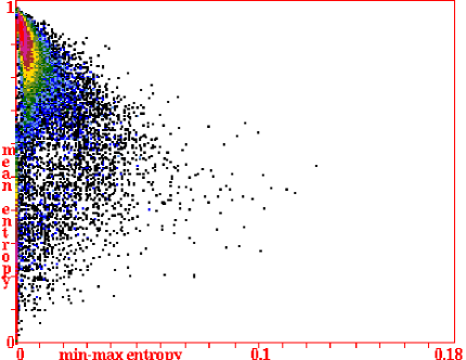
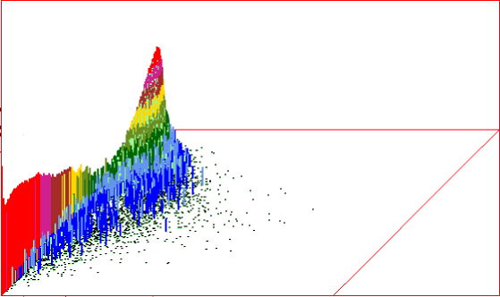
(a) orthogonal lattice $v2k9$, approx density 0/1: seed=70/30, iso-rule=70/30.

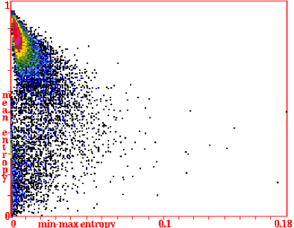
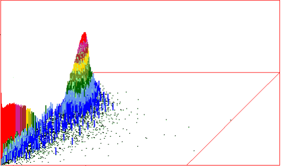
(b) hexagonal lattice $v3k7$, approx density 0/1/2: seed=70/15/15, iso-rule=60,20,20.

Figure 30: Mean-entropy/entropy-variability (min-max) scatter plots based on 2d 60$\times$60 2d the iso-rule IFH. The sample size is 50000, collected overnight on a laptop. (a) $v2k9$ square 2d as for the game-of-Life, and (b) $v3k7$ hex 2d as for the Spiral rule. Left: Each dot represents one or more rules falling within the squares of a 256x256 grid where the x-axis is min-max entropy, y-axis is mean entropy, with dot colors indicating the pile-up frequency. This presentation allows iso-rule-space to be probed to examine the rules and dynamics. Right: with a z-axis showing log₂ rule frequency. Measures were started after 22 initial time-steps and taken over the subsequent 200 time-steps. The approximate densities of the random initial state and the iso-rule are indicated.

Probing various locations of a sorted plot[27, EDD:33.6] with the pointer selects rules or rule patches which can then be listed and run in sequence to see the dynamics, or scanned automatically in blocks of time-steps. Figure 31 shows the locations of characteristic dynamical behaviours.

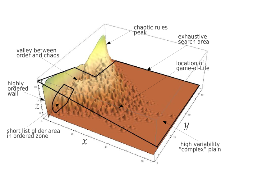
Figure 31: The typical shape of the x-y-z entropy-min-max scatter plot with characteristic dynamical behaviours found in different parts of the landscape and the basis for a probing search avoiding the chaotic peak. The high variability complex plain contains gliders and interacting mobile structures but is unlikely to support glider-guns because of the over-active dynamics and rare stable structure. This figure is taken from our 2015 paper[8] for 93000 isotropic $v2k9$ 2d rules but where the entropy was based on the full 512 rule-table instead of the shorter 102 iso-rule-table in figure 30.

11 summary

Isotropy is arguably the proper canvas for CA logical universality to play out based on glider-gun/eater dynamics, and we have investigated the few such rules we are aware of — the game-of-Life, Sayab, the Spiral rule, and others, some of which were discovered with earlier analogous methods[1, 2, 8, 9, 10, 11].

Isotropic notations for binary CA exist such as the Hensel for Golly[7] and Sapin’s[14, 15], but a general systematic approach to encompass multi-value in one, two and three dimensions was missing, so we have proposed the iso-rule paradigm in this paper. Iso-rules are based on a lookup-table of iso-groups, assemblies of all rotated/reflected neigborhood configurations which can be examined graphically in DDLab. Iso-rules-tables are ordered in the spirit of Wolfram’s classical convention[17, 18].

Iso-rules provide an intermediate granularity between isotropic rules based on full lookup-tables, and isotropic subsets — totalistic, reaction-diffusion and survival/birth rules. DDLab is able to convert these rule types to iso-rules, which then become subject to all DDlab’s other functions[27].

The input-frequency histogram and its mutation/filter game has the potential for investigating the low-level drivers of glider/glider-gun/eater dynamics. Input-entropy and its variability distinguish iso-rules according to ordered/complex/chaotic dynamics, and allow the automatic collection of large samples of classified iso-rule-space to search for new and interesting iso-rules. These method are now available for future research.

12 acknowledgements

Figures and experiments were made with DDLab[28]. J.M. Gómez Soto acknowledges his residency at Discrete Dynamics Lab, and financial support from the Research Council of Mexico (CONACyT).

References

- [1] Adamatzky,A., A.Wuensche, B.De Lacy Costello, “Glider-based computation in reaction-diffusion hexagonal cellular automata”, Chaos, Solitons & Fractals 27, 287–295, 2006. preprint pdf
- [2] Adamatzky,A., and A.Wuensche, “Computing in Spiral Rule Reaction-Diffusion Hexagonal Cellular Automaton”, Complex Systems, Vol 16, 277-297, 2006. preprint pdf
- [3] Berlekamp E,R., J.H.Conway, R.K.Guy, “Winning Ways for Your Mathematical Plays”, Vol 2. Chapt 25 “What is Life?”, 817-850, Academic Press, New York, 1982.
- [4] ConwayLife forum. http://www.conwaylife.com/
- [5] Eppstein,D. “Growth and Decay in Life-Like Cellular Automata”, in Game of Life Cellular Automata, edited by Andrew Adamatzky, Springer Verlag, 2010.
- [6] Gardner,M., ”Mathematical Games – The fantastic combinations of John Conway’s new solitaire game “life”. Scientific American 223. pp. 120–123, 1970.
- [7] Golly Game of Life Home Page. http://golly.sourceforge.net
- [8] Gómez Soto,JM., and A.Wuensche, “The X-rule: universal computation in a non-isotropic Life-like Cellular Automaton”, JCA, Vol 10, No.3-4, 261-294, 2015. arXiv link
- [9] Gómez Soto, J.M., and A.Wuensche, “X-Rule’s Precursor is also Logically Universal”, Journal of Cellular Automata, Vol.12. No.6, 445-473, 2017. arXiv link
- [10] Gómez Soto, J.M., and A.Wuensche, “Logically Universality from a Minimal 2D Glider-Gun”, Complex Systems), vol 27, Issue 1, 2017. arXiv link
- [11] Gómez Soto, J.M., and A.Wuensche, “The Variant-Rule, Another Logically Universal Rule”, Journal of Cellular Automata), to appear, 2020. arXiv link
- [12] Gómez Soto, J.M. web page: “Logical Universality in 2D Cellular Automata”, 2019, link
- [13] Greenberg,J.M., and S.P.Hastings, “Spatial patterns for discrete models of diffusion in excitable media”, SIAM J. Appl. Math. 34, 1978.
- [14] Sapin,E, O. Bailleux, J.J. Chabrier, and P. Collet. “A new universal automata discovered by evolutionary algorithms”, Gecco2004, Lecture Notes in Computer Science, 3102:175187, 2004.
- [15] E. Sapin,E, A. Adamatzky, P. Collet, and L. Bull, “Stochastic automated search methods in cellular automata: the discovery of tens of thousands of glider guns”, Natural Computing 9:513–543, 2010.
- [16] Wojtowicz, Mirek., “What is Life and Cellular Automata?”, 2002. link
- [17] Wolfram,S., “Statistical Mechanics of Cellular Automata”, Reviews of Modern Phisics, vol 55, 601-644, 1983.
- [18] Wolfram,S., “A New Kind of Science”, Wolfram Media, Champaign, IL., 2002.
- [19] Wuensche,A., and M.Lesser, “The global Dynamics of Cellular Automata”, Santa Fe Institute Studies in the Sciences of Complexity, Addison-Wesley, Reading, MA, 1992. link
- [20] Wuensche,A., “Attractor Basins of Discrete Networks; Implications on self-organisation and memory”, Cognitive Science Research Paper 461, Univ. of Sussex, D.Phil thesis, 1997. link
- [21] Wuensche,A., “Classifying Cellular Automata Automatically; Finding gliders, filtering, and relating space-time patterns, attractor basins, and the Z parameter”, COMPLEXITY, Vol.4/no.3, 47-66, 1999. preprint pdf
- [22] Wuensche,A., “Glider Dynamics in 3-Value Hexagonal Cellular Automata: The Beehive Rule”, Int. Journ. of Unconventional Computing, Vol.1, No.4, 375-398, 2005. preprint pdf
- [23] Wuensche,A., Beehive rule webpage (2006). link
- [24] Wuensche,A., A.Adamatzky, “On spiral glider-guns in hexagonal cellular automata: activator-inhibitor paradigm”, International Journal of Modern Physics C, Vol.17, No.7, 1009-1026, 2006. preprint pdf
- [25] Wuensche,A., Spiral rule webpage (2006). link
- [26] Wuensche,A., E.C.Coxon (2018), “The cellular automaton pulsing model, experiments with DDLab”, ACTA PHYSICA POLONICA, vol.12, 135-154. arXiv link
- [27] Wuensche,A.,“Exploring Discrete Dynamics – Second Edition, Luniver Press, 2016. Online pdf update Feb 2021. link
-
[28]
Wuensche,A., Discrete Dynamics Lab (DDLab), 1993-2021.
http://www.ddlab.org - [29] Wuensche,A., online DDLab isotropic rule update Jan 2018. link
- [30] Wuensche,A., online DDLab iso-rule update Feb 2021. link