Structure exploiting methods for fast uncertainty quantification in multiphase flow through heterogeneous media

Abstract

We present a computational framework for dimension reduction and surrogate modeling to accelerate uncertainty quantification in computationally intensive models with high-dimensional inputs and function-valued outputs. Our driving application is multiphase flow in saturated-unsaturated porous media in the context of radioactive waste storage. For fast input dimension reduction, we utilize an approximate global sensitivity measure, for function-valued outputs, motivated by ideas from the active subspace methods. The proposed approach does not require expensive gradient computations. We generate an efficient surrogate model by combining a truncated Karhunen-Loéve (KL) expansion of the output with polynomial chaos expansions, for the output KL modes, constructed in the reduced parameter space. We demonstrate the effectiveness of the proposed surrogate modeling approach with a comprehensive set of numerical experiments, where we consider a number of function-valued (temporally or spatially distributed) QoIs.

1 Introduction

Low permeability argillites are considered as suitable host rocks for underground radioactive waste storage to retain radionuclides locally. However, hydrogen gas produced by corrosion of steel engineered barriers can represent a threat to the installation safety. A significant impact of this production is the overpressurization of hydrogen around alveolus leading to opening fractures in the surrounding host rock and inducing groundwater flow and transport of radionuclides outside of the geological repositories. This problem renews the mathematical interest in the equations describing multiphase multicomponent flows through porous media, within the present context. An important aspect of improving the prediction fidelity of such models is to account for the various sources of uncertainty in the governing equations.

Performing uncertainty analysis on the models under study using a direct Monte Carlo sampling approach is infeasible. This is due to the high cost of model simulations and the need for a large number of such simulations. Therefore, there is a need for quick-to-evaluate surrogate models that accurately capture the underlying physics and statistical properties of the quantities of interest (QoIs). Surrogate modeling, however, is a formidable task for the applications considered in the present work. Models describing flow through porous media exhibit distinct challenges with regards to uncertainty quantification and surrogate modeling including expensive simulations, high-dimensional uncertain parameters, and function-valued outputs. Addressing these challenges effectively requires understanding and exploiting the problem structure. To this end, we propose a framework that deploys a sensitivity analysis approach to reduce the dimensionality of the input parameter and utilizes the spectral properties of the output QoI to generate an efficient surrogate model.

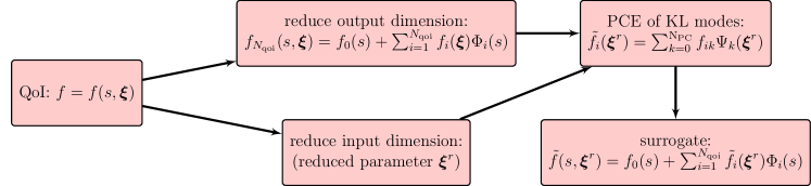
Figure 1: A schematic of the proposed bispectral surrogate modeling approach.

Related work. The modeling of underground radioactive waste storage involves simulating the coupled transport of multiphase multicomponent flow in porous medium. Equations governing this type of flow in porous media are nonlinear and involve simulation of complex phenomena such as the appearance and the disappearance of the gas phase leading to the degeneracy of the equations satisfied by the saturation. There have been significant research efforts dealing with mathematical and numerical models for simulating the transport migration of radionuclides. The articles Bourgeat2012 ; Bourgeat2009 present test-cases and set up benchmark examples to address some of the specific problems encountered when numerically simulating gas migration in underground nuclear waste repositories. In Angelini2011 ; Bourgeat2009 ; Neumann2012 different choices of primary variables have been proposed to tackle the degeneracy of the equations satisfied by the saturation. In Saad2020 , the authors study a compressible and partially miscible phase flow model in porous media, applied to gas migration in an underground nuclear waste repository in the case where the velocity of the mass exchange between dissolved hydrogen and hydrogen in the gas phase is supposed finite. Also presented is a numerical scheme based on a two-step convection/diffusion-relaxation strategy to simulate the non-equilibrium model. There have also been efforts to quantify uncertainty in models of multiphase flow ChristieDemyanovErbas06 ; Najm09 ; NamhataOladyshkinDilmore16 ; SaadAlexanderianPrudhommeEtAl18 ; SeverinoLevequeToraldo19 ; XiaoOladyshkinNowak19 .

The tools from uncertainty quantification that are relevant to the present work include global sensitivity analysis (GSA) and surrogate modeling. GSA provides insight into how uncertainties in model parameters influence model outputs by identifying the input parameters a QoI is sensitive to. This increases overall understanding of the underlying physics and guides parameter dimension reduction. The Sobol’ indices Sobol01 , derivative-based global sensitivity measures (DGSMs) KucherenkoRodriguez09 ; KucherenkoIooss17 ; SobolKucherenko09 , and active subspace methods Constantine15 ; ConstantineDiaz17 are examples of GSA tools widely used in practice. These concepts were originally conceived for scalar QoIs. Recent works such as AlexanderianGremaudSmith20 ; CleavesAlexanderianGuyEtAl19 ; ZahmConstantine2020 generalize standard GSA tools to the case of vector- and function-valued QoIs. In particular, GamboaJanonKlein14 ; AlexanderianGremaudSmith20 concern variance-based GSA using Sobol’ indices for such QoIs. The article CleavesAlexanderianGuyEtAl19 studies DGSMs for function-valued QoIs. A generalization of active subspace methods for vectorial outputs is presented in ZahmConstantine2020 .

For expensive-to-compute QoIs calculating GSA measures such as Sobol’ indices is computationally expensive. A common method for mitigating the computational cost is to construct a cheap-to-evaluate surrogate model for the QoI and then apply GSA techniques to the surrogate. For example, polynomial chaos expansions (PCEs) have been a popular approach for accelerating the computation of Sobol’ indices; see, e.g., AlexanderianWinokurSrajEtAl12 ; BlatmanetAl2010 ; Crestaux09 ; Sudret08 . Surrogate model construction, however, is itself a computationally challenging task, especially in the case of models with high-dimensional input parameters. For such models it is also possible to use a multilevel approach: initial parameter screening can be performed using cheap, but less precise, tools and further dimension reduction is performed through more rigorous methods such as a variance-based analysis using accurate surrogate models constructed in a reduced-dimensional parameter space; see e.g., HartGremaudDavid19 .

For function-valued QoIs, a straightforward approach is to compute surrogate models for every grid point in a discretized computational domain. This approach, however, can be inefficient and ignores an important problem structure—the low-rank structure of the output. Specifically, in many applications, function-valued QoIs can be represented via a spectral representation, such as a Karhunen–Loéve expansion (KLE), with a small number of terms. This problem structure can be exploited for surrogate modeling: instead of approximating a field quantity at every point in a computational grid, one can approximate a few dominant modes of the output QoI. Such surrogate models can also be used to accelerate GSA methods; see e.g., AlexanderianGremaudSmith20 ; CleavesAlexanderianGuyEtAl19 ; GuyetAl19 ; LiIskandaraniLeHenaff16 .

Our approach and contributions.

In the present work, we seek to construct surrogate models for fast analysis of computationally intensive models with high-dimensional parameters and function-valued QoIs. We consider QoIs of the form

$$f=f(s,{\mathchoice{\mbox{\boldmath$\displaystyle{\xi}$}}{\mbox{\boldmath$\textstyle{\xi}$}}{\mbox{\boldmath$\scriptstyle{\xi}$}}{\mbox{\boldmath$\scriptscriptstyle{\xi}$}}}),\quad s\in\mathscr{X},\,{\mathchoice{\mbox{\boldmath$\displaystyle{\xi}$}}{\mbox{\boldmath$\textstyle{\xi}$}}{\mbox{\boldmath$\scriptstyle{\xi}$}}{\mbox{\boldmath$\scriptscriptstyle{\xi}$}}}\in\Theta,$$

where $\Theta\subseteq\mathbb{R}^{{{N}_{\text{p}}}}$ is the uncertain parameter domain and $\mathscr{X}$ is compact subset of $\mathbb{R}^{d}$, with $d\in\{1,2,3\}$. In practice, $s$ can represent a spatial or temporal point. Our focus in the present work is models of flow in porous media, and $f(s,{\mathchoice{\mbox{\boldmath$\displaystyle{\xi}$}}{\mbox{\boldmath$\textstyle{\xi}$}}{\mbox{\boldmath$\scriptstyle{\xi}$}}{\mbox{\boldmath$\scriptscriptstyle{\xi}$}}})$ is an observable in a multiphase flow problem. Our approach identifies and exploits low-dimensional structures in both input and output spaces. Specifically, we rely on approximate GSA measures for fast input parameter screening and utilize low-rank spectral representations of output fields.

We propose a fast-to-compute screening metric that utilizes ideas from active subspaces Constantine15 and derivative-based GSA for functional outputs CleavesAlexanderianGuyEtAl19 to perform parameter dimension reduction. The proposed screening metrics do not require gradient computation in the parameter space. This makes the proposed methods applicable to a broad class of problems involving complex physics systems for which adjoint solvers, which are essential for gradient computation in high dimensions, are not necessarily available.

Following parameter screening, we combine two different spectral approaches—KLEs and PCEs—to generate an efficient surrogate model in a reduced-dimensional uncertain parameter space. The overall surrogate model constructed takes the form,

$$f_{{{{{N}_{\text{qoi}}}}\!}}^{{\text{PC}}}(s,{\mathchoice{\mbox{\boldmath$\displaystyle{\xi}$}}{\mbox{\boldmath$\textstyle{\xi}$}}{\mbox{\boldmath$\scriptstyle{\xi}$}}{\mbox{\boldmath$\scriptscriptstyle{\xi}$}}}^{r})=f_{0}(s)+\sum_{i=1}^{{N}_{\text{qoi}}}f_{i}^{\text{PC}}({\mathchoice{\mbox{\boldmath$\displaystyle{\xi}$}}{\mbox{\boldmath$\textstyle{\xi}$}}{\mbox{\boldmath$\scriptstyle{\xi}$}}{\mbox{\boldmath$\scriptscriptstyle{\xi}$}}}^{r})\Phi_{i}(s),$$

where $\Phi_{i}$’s are orthogonal basis functions in $L^{2}(\mathscr{X})$ obtained from a KLE of $f(s,{\mathchoice{\mbox{\boldmath$\displaystyle{\xi}$}}{\mbox{\boldmath$\textstyle{\xi}$}}{\mbox{\boldmath$\scriptstyle{\xi}$}}{\mbox{\boldmath$\scriptscriptstyle{\xi}$}}})$ and $f_{i}^{PC}$ are approximate KL modes as functions of a reduced-dimensional parameter vector ${\mathchoice{\mbox{\boldmath$\displaystyle{\xi}$}}{\mbox{\boldmath$\textstyle{\xi}$}}{\mbox{\boldmath$\scriptstyle{\xi}$}}{\mbox{\boldmath$\scriptscriptstyle{\xi}$}}}^{r}\subseteq\mathbb{R}^{{n}_{\text{p}}}$; these KL modes are represented by PCEs,

$$f_{i}^{\text{PC}}({\mathchoice{\mbox{\boldmath$\displaystyle{\xi}$}}{\mbox{\boldmath$\textstyle{\xi}$}}{\mbox{\boldmath$\scriptstyle{\xi}$}}{\mbox{\boldmath$\scriptscriptstyle{\xi}$}}}^{r})=\sum_{k=0}^{{N}_{\text{PC}}}f_{ik}\Psi_{k}({\mathchoice{\mbox{\boldmath$\displaystyle{\xi}$}}{\mbox{\boldmath$\textstyle{\xi}$}}{\mbox{\boldmath$\scriptstyle{\xi}$}}{\mbox{\boldmath$\scriptscriptstyle{\xi}$}}}^{r}),$$

where $\Psi_{k}$’s are a basis consisting of multivariate orthogonal polynomials in $L^{2}(\Theta)$ and ${N}_{\text{PC}}$ is specified based on the choice of truncation strategy. Thus, the overall surrogate model can be expressed as

$$f(s,{\mathchoice{\mbox{\boldmath$\displaystyle{\xi}$}}{\mbox{\boldmath$\textstyle{\xi}$}}{\mbox{\boldmath$\scriptstyle{\xi}$}}{\mbox{\boldmath$\scriptscriptstyle{\xi}$}}})\approx f_{0}(s)+\sum_{i=1}^{{N}_{\text{qoi}}}\sum_{k=0}^{{N}_{\text{PC}}}f_{ik}\Psi_{k}({\mathchoice{\mbox{\boldmath$\displaystyle{\xi}$}}{\mbox{\boldmath$\textstyle{\xi}$}}{\mbox{\boldmath$\scriptstyle{\xi}$}}{\mbox{\boldmath$\scriptscriptstyle{\xi}$}}}^{r})\Phi_{i}(s).$$ (1)

We refer to the class of surrogate models of the form (1) as bispectral surrogates due to the use of spectral representations in $L^{2}(\mathscr{X})$ and $L^{2}(\Theta)$. In Figure 1, we provide a schematic of the proposed bispectral surrogate modeling framework. We point out that the proposed approach is non-intrusive and requires only the ability to evaluate the governing model at a sample of uncertain inputs. See Section 5 for details.

While computing a surrogate model from a truncated KLE by replacing the KL modes with PCEs (or other surrogates) is not new, see e.g., AlexanderianGremaudSmith20 ; GuyetAl19 ; LiIskandaraniLeHenaff16 , we build upon this approach by including a gradient-free input dimension reduction approach as a first step. This enables the PCEs for the KL modes to be built in a lower-dimensional space. Thus, a major contribution of this article is a synergy of known techniques combined with a novel input dimension reduction strategy to furnish an integrated surrogate modeling approach. We also provide a detailed computational procedure for the proposed framework, making the present work a self-contained guide. We elaborate our approach on an intricate multiphase multicomponent flow model for which a comprehensive presentation is also given. In our numerical results, we implement the proposed approach for both spatially- and temporally-varying QoIs. Additionally, a variety of statistical studies are conducted with the constructed bispectral surrogate. These tests are intended to showcase the versatility of the surrogate model and explore the physical phenomenon under study. In particular, we perform model predictions, compute variance-based global sensitivity indices, and study statistical model response behavior. In addition to demonstrating the effectiveness of the proposed strategy, our computational results provide valuable insight regarding the response of complex porous media flow models to uncertainties in material properties.

Article overview. In section 2 we present a detailed overview of the multiphase multicomponent flow model that is central to the present work. We also provide a description of our choice of numerical solver for the governing equations. In section 3, we discuss modeling the uncertainties in material properties, as well as give a brief explanation of the model response and relevant QoIs. We supply a concise overview of KLEs, PCEs, and bispectral surrogates in section 4. In section 5 we provide a detailed framework, including algorithms, for the proposed dimension reduction and surrogate modeling approach. Our computational results are presented in section 6. Finally, we provide closing comments in section 7.

2 Model Description

2.1 Mathematical formulation of the continuous problem

Here we state the physical model used in this work. We consider a porous medium saturated with a fluid composed of two phases, liquid ($l$) and gas ($g$), and a mixture of two components, water ($w$) and hydrogen ($h$). The spatial domain $\Omega$ is a bounded open subset of $\mathbb{R}^{\ell}$ ($\ell=1,2$, or $3$) and the problem is considered in the time interval $[0,T_{f}]$, where $T_{f}>0$ is the final time. To define the physical model, we write the mass conservation of each component in each phase

$$\phiup\partial_{t}(\rho_{l}^{w}S_{\!l} +\rho_{g}^{w}S_{\!g})$$

$$+\nabla\cdot(\rho_{l}^{w}\textbf{V}_{l}+\rho_{g}^{w}\textbf{V}_{g}+{\mathchoice{\mbox{\boldmath$\displaystyle{J}$}}{\mbox{\boldmath$\textstyle{J}$}}{\mbox{\boldmath$\scriptstyle{J}$}}{\mbox{\boldmath$\scriptscriptstyle{J}$}}}_{l}^{w}+{\mathchoice{\mbox{\boldmath$\displaystyle{J}$}}{\mbox{\boldmath$\textstyle{J}$}}{\mbox{\boldmath$\scriptstyle{J}$}}{\mbox{\boldmath$\scriptscriptstyle{J}$}}}_{g}^{w})=f^{w},$$ (2)

$$\phiup\partial_{t}(\rho_{l}^{h}S_{\!l} +\rho_{g}^{h}S_{\!g})$$

$$+\nabla\cdot(\rho_{l}^{h}\textbf{V}_{l}+\rho_{g}^{h}\textbf{V}_{g}+{\mathchoice{\mbox{\boldmath$\displaystyle{J}$}}{\mbox{\boldmath$\textstyle{J}$}}{\mbox{\boldmath$\scriptstyle{J}$}}{\mbox{\boldmath$\scriptscriptstyle{J}$}}}_{l}^{h}+{\mathchoice{\mbox{\boldmath$\displaystyle{J}$}}{\mbox{\boldmath$\textstyle{J}$}}{\mbox{\boldmath$\scriptstyle{J}$}}{\mbox{\boldmath$\scriptscriptstyle{J}$}}}_{g}^{h})=f^{h},$$ (3)

where $\phiup(x)$ is the given porosity of the medium, $S_{\!\alpha}(t,x)$ the saturation of the phase $\alpha\in\{l,g\}$, with the two saturations summing to one. Also, $p_{\alpha}(t,x)$ is the pressure of the phase $\alpha$, $\rho_{\alpha}^{\beta}$ is the density of the component $\beta\in\{w,h\}$ in the phase $\alpha$, and $\rho_{\alpha}=\rho_{\alpha}^{h}+\rho_{\alpha}^{w}$ is the density of the phase $\alpha$. The velocity of each fluid, $\textbf{V}_{\alpha}$ is given by Darcy’s law

$$\textbf{V}_{\alpha}=-{\bf K}\frac{k_{r_{\alpha}}(S_{\!\alpha})}{\mu_{\alpha}}\big{(}\nabla p_{\alpha}-\rho_{\alpha}(p_{\alpha})\textbf{g}\big{)},$$

where ${\bf K}(x)$ is the intrinsic (given) permeability tensor of the porous medium, $k_{r_{\alpha}}$ the relative permeability of the $\alpha$-phase, $\mu_{\alpha}$ the constant $\alpha$-phase’s viscosity, $p_{\alpha}$ the $\alpha$-phase’s pressure, and g, the gravity vector. For further details of the model we refer to the presentation of the benchmark Bourgeat2012 ; Bourgeat2009 . Following the Fick’s law, the diffusive flux of a component $\beta$ in the phase $\alpha$ is given by

$${\mathchoice{\mbox{\boldmath$\displaystyle{J}$}}{\mbox{\boldmath$\textstyle{J}$}}{\mbox{\boldmath$\scriptstyle{J}$}}{\mbox{\boldmath$\scriptscriptstyle{J}$}}}_{\alpha}^{\beta}=-\phiup S_{\!\alpha}\rho_{\alpha}D_{\alpha}^{\beta}\nabla\mathcal{X}_{\alpha}^{\beta},$$

where coefficient $D_{\alpha}^{\beta}$ is the Darcy scale molecular diffusion coefficients of $\beta$-component in $\alpha$-phase and $\mathcal{X}_{\alpha}^{\beta}={\rho_{\alpha}^{\beta}}/{\rho_{\alpha}}$ is the component $\beta$ molar fraction in phase $\alpha$. Diffusive fluxes satisfy $\sum_{\beta}{\mathchoice{\mbox{\boldmath$\displaystyle{J}$}}{\mbox{\boldmath$\textstyle{J}$}}{\mbox{\boldmath$\scriptstyle{J}$}}{\mbox{\boldmath$\scriptscriptstyle{J}$}}}_{\alpha}^{\beta}=0$ for each $\alpha$.

The capillary pressure law, which links the jump of pressure of the two phases to the saturation, is

$$p_{c}(S_{\!l})=p_{g}-p_{l}.$$

This function is decreasing ($\frac{\text{d}p_{c}}{\text{d}S_{\!l}}(S_{\!l})<0\text{ for all }S_{\!l}\in[0,1]$), and satisfies $p_{c}(1)=0$.

In the present work, the water is supposed only present in the liquid phase (no vapor of water due to evaporation). Thus, (2)–(3) could be rewritten as

$$\phiup\partial_{t}(S_{\!l}\,\rho_{l}^{w}) +\nabla\cdot(\rho_{l}^{w}\textbf{V}_{l})$$

$$+\nabla\cdot(\phiup S_{\!l}\,\rho_{l}D_{l}^{h}\nabla X_{l}^{h})=f^{w},$$ (4)

$$\phiup\partial_{t}(S_{\!l}\,\rho_{l}^{h}+S_{\!g}\,\rho_{g}^{h}) +\nabla\cdot(\rho_{l}^{h}\textbf{V}_{l}+\rho_{g}^{h}\textbf{V}_{g})$$

$$-\nabla\cdot(\phiup S_{\!l}\,\rho_{l}D_{l}^{h}\nabla X_{l}^{h})=f^{h}.$$ (5)

The system (4)–(5) is not complete; to close the system, we use the ideal gas law and the Henry’s law

$$\rho_{g}^{h}=\frac{M^{h}}{RT}p_{g}\quad\text{and}\quad\rho_{l}^{h}=M^{h}H^{h}p_{g},$$ (6)

where the quantities $M^{h}$, $H^{h}$, $R$ and $T$ represent respectively the molar mass of hydrogen, the Henry’s constant for hydrogen, the universal constant of perfect gases and $T$ the temperature. By these formulation, the system (4)–(5) is closed and we choose the liquid pressure and the density of dissolved hydrogen as unknowns. From (6), the Henry’s law combined to the ideal gas law, to obtain that the density of hydrogen gas is proportional to the density of hydrogen dissolved

$$\rho_{g}^{h}=\mathcal{C}\rho_{l}^{h}\quad\text{where}\quad\mathcal{C}=\frac{1}{H_{h}RT}=52.51.$$

Note that the density of water $\rho_{l}^{w}$ in the liquid phase is constant and from the Henry’s law, we can write

$$\rho_{l}\nabla\mathcal{X}_{l}^{h}=\mathcal{X}_{l}^{w}\nabla\rho_{l}^{h}.$$

Then the system (4)–(5) can be written as

$$\phiup\partial_{t}\left(S_{\!l}\,\rho_{l}^{w}\right) +\nabla\cdot\left(\rho_{l}^{w}\textbf{V}_{l}\right)$$

$$+\nabla\cdot\left(\phiup S_{\!l}\,\mathcal{X}_{l}^{w}D_{l}^{h}\nabla\rho_{l}^{h}\right)=f^{w},$$

$$\phiup\partial_{t}\left(m(S_{\!l})\rho_{l}^{h}\right) +\nabla\cdot\left(\rho_{l}^{h}\textbf{V}_{l}+\mathcal{C}\rho_{l}^{h}\textbf{V}_{g}\right)$$

$$-\nabla\cdot\left(\phiup S_{\!l}\,\mathcal{X}_{l}^{w}D_{l}^{h}\nabla\rho_{l}^{h}\right)=f^{h},$$

where $m(S_{\!l})=S_{\!l}+\mathcal{C}S_{\!g}$.

A van Genuchten-Mualem model with the parameters $n$, $S_{\!\alpha r}$ and $p_{r}$ as given in Table 1 (left) is used for the relative permeabilities and capillary pressure:

$$p_{c}(S_{\!le}) =p_{r}\left(S_{\!le}^{-1/\upsilon}-1\right)^{1/n},$$

$$k_{r_{l}}(S_{\!le}) =\sqrt{S_{\!le}}\left(1-\left(1-S_{\!le}^{1/\upsilon}\right)^{\upsilon}\right)^{2},$$

$$k_{r_{g}}(S_{\!le}) =\sqrt{1-S_{\!le}}\left(1-S_{\!le}^{1/\upsilon}\right)^{2\upsilon},$$

with the effective saturation

$$S_{\!le}=(S_{\!l}-S_{\!lr})/(1-S_{\!lr}-S_{\!gr}),$$

where $S_{\!lr}$ and $S_{\!gr}$ are the liquid and gas residual saturations, respectively, and $\upsilon=1-1/n$.

2.2 Numerical solver

As is well known, the modeling of underground radioactive waste storage involves simulation of complex phenomena such as the appearance and the disappearance of the gas phase leading to the degeneracy of the equations satisfied by the saturation. This is mainly due to the migration of gas produced by the corrosion of nuclear waste packages within a complex heterogeneous domain. To overcome this difficulty, an important consideration, in the modelling of multiphase flow with mass exchange between phases, is the choice of the primary variables that define the thermodynamic state of the system. Different choices of primary variables have been proposed  Angelini2011 ; Bourgeat2009 ; Neumann2012 . In this article, we consider pressure of the liquid phase and density of dissolved hydrogen the primary unknowns in the multiphase flow system. A cell-centered finite volume scheme is used for the space discretization and an implicit Euler scheme for the temporal discretization. The nonlinear system is solved with a fixed point method.

In this section, we present a numerical study dedicated to understanding the computational issues caused by gas phase appearance produced by injecting of hydrogen in a one-dimensional homogeneous porous domain. We consider a domain that is fully saturated with water. This numerical study is inspired by the MoMaS benchmark on multiphase flow in porous media Bourgeat2012 .

2.3 Numerical experiment

We consider a one-dimensional domain with the benchmark setup described in Bourgeat2012 . The spatial domain $\Omega$ is the interval $(0,L)$, with $L=200$ meters, and the final simulation time is $T_{f}=10^{6}$ years. The parameters for porous medium, fluid characteristics, and initial and boundary conditions are presented in Bourgeat2012 and summarized in Table 1.

Table 1: Left: parameter values for the porous medium and fluid characteristics used in test case 1. Right: parameter values for domain size, boundary and initial conditions, total injection time and total simulation time.

Parameter Value Parameter Value $\phiup$ [-] 0.15 $D_{l}^{h}$ [$\mathrm{m^{2}\cdot s^{-1}}$] $3\times 10^{-9}$ ${\bf K}$ [$\mathrm{m^{2}}$] $5\times 10^{-20}$ $\mu_{l}$ [$\mathrm{Pa\cdot s}$] $1\times 10^{-3}$ $p_{r}$ [$\mathrm{Pa}$] $2\times 10^{6}$ $\mu_{g}$ [$\mathrm{Pa\cdot s}$] $9\times 10^{-6}$ $n$ [-] $1.54$ $H^{h}$ [$\mathrm{mol.Pa^{-1}.m^{-3}}$] $7.65\times 10^{-6}$ $S_{lr}$ [-] $0.4$ $M^{h}$ [$\mathrm{Kg\cdot mol^{-1}}$] $2\times 10^{-3}$ $S_{gr}$ [-] $0$ $\rho_{l}^{w}$ [$\mathrm{Kg\cdot mol^{-3}}$] $10^{3}$

Parameter Value $L$ [$\mathrm{m}$] 200 $q_{h}$ [$\mathrm{kg/m^{2}/year}$] $5.57\times 10^{-6}$ $p_{init}$ [$\mathrm{Pa}$] $10^{6}$ $T_{inj}$ [$\mathrm{years}$] $5\times 10^{5}$ $T_{f}$ [$\mathrm{years}$] $10^{6}$

Initial conditions are uniform over the whole domain with pure liquid water at fixed liquid pressure and no hydrogen present,

$$p_{l}(0,x)=p_{init}\quad\text{and}\quad\rho_{l}^{h}(0,x)=0,\quad x\in\Omega.$$

For boundary conditions, a constant flux of hydrogen and zero water flow rate were imposed on the left boundary

$$\rho_{l}^{w}V_{l}-J_{l}^{h} =0,$$

$$\rho_{l}^{h}V_{l}+\rho_{g}^{h}V_{g}+J_{l}^{h} =\begin{cases}q_{h}\quad 0\leq t\leq T_{\text{inj}},\\ 0\quad t>T_{\text{inj}}.\end{cases}$$

On the right boundary, Dirichlet boundary conditions the same as the initial conditions are imposed.

To validate our solver, we run simulations with the nominal parameters and report the phase pressures and gas saturation at the inflow boundary. Our results are consistent with those reported in Angelini2011 ; Bourgeat2009 ; Neumann2012 . Figure 2 shows the gas saturation (top) and the phase pressures (bottom), with respect to time (years) during and after injection. For $0<t<13\times 10^{3}$ years, the gas saturation remains zero, all injected hydrogen dissolves into the liquid phase, the whole domain is saturated with water, and the liquid pressure remains constant. At $t\approx 13\times 10^{3}$ years, the maximum solubility is reached and the gas phase appears at the injection boundary. Gas saturation keeps growing during the period of hydrogen injection. When injection stops at $t=5\times 10^{5}$ years, gas saturation decreases until it disappears. A negative water flux is observed (see Figure 3) as water comes from right to left to fill in the empty space. At the end of the simulation, the gas pressure continues to decrease and the liquid pressure gradient goes to zero, as the system reaches a steady state.

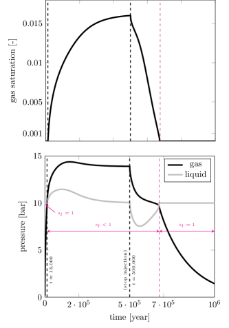
Figure 2: Gas saturation (top) and liquid and gas pressures (bottom) at the inflow boundary.

Figure 3: Liquid (top) and gas (bottom) flux at the outflow boundary.

3 Modeling under uncertainty

We seek to understand the impact of uncertainty in heterogeneous material properties on model predictions. Specifically, we focus on uncertainties in porosity and absolute permeability. Our goal is to understand the impact of uncertainties in material properties on the gas phase appearance/disappearance in a two phase flow produced by hydrogen injection through a porous medium, which is initially fully saturated with water.

3.1 Modeling uncertainty in material properties

While in the setup of the benchmark problem constant values for porosity and permeability were used, allowing for spatially varying porosity and permeability provides a more realistic representation. This leads to representation of these quantities as random fields.

We model the porosity, $\phiup$, as a random field as follows. Let $Z(x,\omega)$ be a Gaussian process, with exponential covariance function $c(x,y)=e^{-|x-y|/\ell}$, where $\ell>0$ is the correlation length. We chose $\ell=10$ $\mathrm{m}$ (recall the length of the domain is $200$ $\mathrm{m}$). The covariance operator of $Z$ is defined by

$$[\mathcal{C}_{\text{par}}u](x)=\int_{\Omega}c(x,y)u(y)\,dy,\quad u\in L^{2}(\Omega).$$ (8)

We define the random porosity field by

$$\phiup(x,\omega)=F_{B}^{-1}\left(F_{G}(Z(x,\omega));\alpha_{\text{beta}},\beta_{\text{beta}}\right).$$ (9)

Here $F_{B}^{-1}(\cdot;\alpha_{\text{beta}},\beta_{\text{beta}})$ is the inverse CDF of a Beta$(\alpha_{\text{beta}},\beta_{\text{beta}})$ distribution and $F_{G}$ is the CDF of a standard normal distribution. This ensures that for every $x\in\Omega$ the porosity is distributed according to Beta$(\alpha_{\text{beta}},\beta_{\text{beta}})$. The random permeability field is obtained using a Kozeny–Carman relation Costa06 ; Lie19 :

$$K(\phiup)\propto\frac{\phiup^{3}}{(1-\phiup)^{2}}.$$

We set the proportionality constant in the above relation so that $K(\bar{\phiup})=\bar{K}$, where $\bar{\phiup}$ and $\bar{K}$ are the nominal porosity and permeability values listed in Table 1 (left). The values of $\alpha_{\text{beta}}$ and $\beta_{\text{beta}}$ in (9) are set such that the mode of the porosity distribution (at each $x\in\Omega$) is the nominal porosity of $\bar{\phiup}=0.15$. Specifically, we chose $\alpha_{\text{beta}}=20$ and found $\beta_{\text{beta}}$ from the formula for the mode of a Beta distribution: $(\alpha_{\text{beta}}-1)/(\alpha_{\text{beta}}+\beta_{\text{beta}}-2)=\bar{\phiup}$. We depict the distributions for pointwise porosity and permeability values along with the porosity permeability relation in Figure 4 (top). We note that the present setup provides a physically meaningful range of values for porosity and permeability, for the application problem under study.

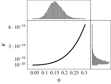
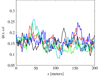
Figure 4: Top: the porosity permeability relation and the distributions of pointwise porosity and permeability. Bottom: a few realizations of the porosity field.

To facilitate uncertainty quantification, we consider a truncated KLE of the Gaussian random field $Z(x,\omega)$ used in definition of $\phiup(x,\omega)$ in (9). That is, we consider

$$Z(x,\omega)\approx\sum_{i=1}^{{N}_{\text{p}}}\sqrt{\lambda}_{i}\xi_{i}e_{i}(x),$$ (10)

where $(\lambda_{i},e_{i})$, $i=1,\ldots,{{N}_{\text{p}}}$ are the eigenpairs of the covariance operator of $Z(x,\omega)$; see e.g., AlexanderianReeseSmithEtAl18 ; BetzPapaioannouStraub14 ; Maitre10 for details about the use of KL expansions for representing random fields in mathematical models. For the present problem, we let ${{N}_{\text{p}}}=100$, which enables capturing over $96$ percent of the average variance of the process. Notice that with the present setup, the uncertainty in the porosity field is fully captured by the vector ${\mathchoice{\mbox{\boldmath$\displaystyle{\xi}$}}{\mbox{\boldmath$\textstyle{\xi}$}}{\mbox{\boldmath$\scriptstyle{\xi}$}}{\mbox{\boldmath$\scriptscriptstyle{\xi}$}}}=[\begin{matrix}\xi_{1}&\xi_{2}&\cdots&\xi_{{N}_{\text{p}}}\end{matrix}]^{\mkern-1.5mu\mathsf{T}}$, where $\xi_{i}$’s are the KLE coefficients in (10), which are independent standard normal random variables. As an illustration, we show a few realizations of the random porosity field in Figure 4 (bottom).

3.2 The QoIs under study

We focus on dynamics of hydrogen in gas phase by considering on the time evolution of gas saturation and pressure at the inflow boundary and gas flux at the outflow boundary. The units for gas pressure and gas flux are [$\mathrm{b}\mathrm{a}\mathrm{r}$] and [$\mathrm{k}\mathrm{g}\mathrm{/}\mathrm{m}^{2}\mathrm{/}{year}$], respectively. These time-dependent QoIs are indeed random field quantities due to randomness in porosity and permeability fields. Notice that since the uncertainty in porosity field is encoded in the coefficients $\textstyle{\xi}$ in (10), the randomness in these QoIs is also parameterized by the vector $\textstyle{\xi}$ of the KL coefficients. We denote the uncertain gas saturation at the inflow boundary and gas flux at the outflow boundary by $S(t,{\mathchoice{\mbox{\boldmath$\displaystyle{\xi}$}}{\mbox{\boldmath$\textstyle{\xi}$}}{\mbox{\boldmath$\scriptstyle{\xi}$}}{\mbox{\boldmath$\scriptscriptstyle{\xi}$}}})$, and $Q(t,{\mathchoice{\mbox{\boldmath$\displaystyle{\xi}$}}{\mbox{\boldmath$\textstyle{\xi}$}}{\mbox{\boldmath$\scriptstyle{\xi}$}}{\mbox{\boldmath$\scriptscriptstyle{\xi}$}}})$, respectively. In Figure 5, we depict a few realizations of these uncertain QoIs.

We also consider the gas saturation throughout the domain, at various points in time. We denote this QoI by $S(x,{\mathchoice{\mbox{\boldmath$\displaystyle{\xi}$}}{\mbox{\boldmath$\textstyle{\xi}$}}{\mbox{\boldmath$\scriptstyle{\xi}$}}{\mbox{\boldmath$\scriptscriptstyle{\xi}$}}};t^{*})$, where $t^{*}$ is a fixed time. Figure 6 shows a few realizations of this QoI at $t^{*}=300{,}091$ years. To further illustrate the impact of spatial heterogeneity on the flow model, we also report a plot of the gas saturation in the space-time domain in Figure 7.

Performing statistical studies and predictions on the QoIs outlined above is challenging due to the high cost of solving the governing equations and the high-dimensionality of the input and output spaces. A major aim of this article is to present a surrogate modelling framework that approximates the time- or space-dependent QoIs efficiently by reducing the input and output dimensions and using suitable approximations.

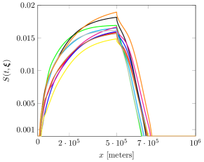
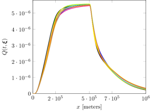
Figure 5: A few realizations of the time evolution of top: gas saturation at the inflow boundary, bottom: gas flux at the outflow boundary.

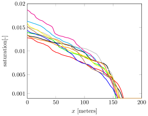
Figure 6: Gas saturation at $t^{*}=300{,}091$ years.

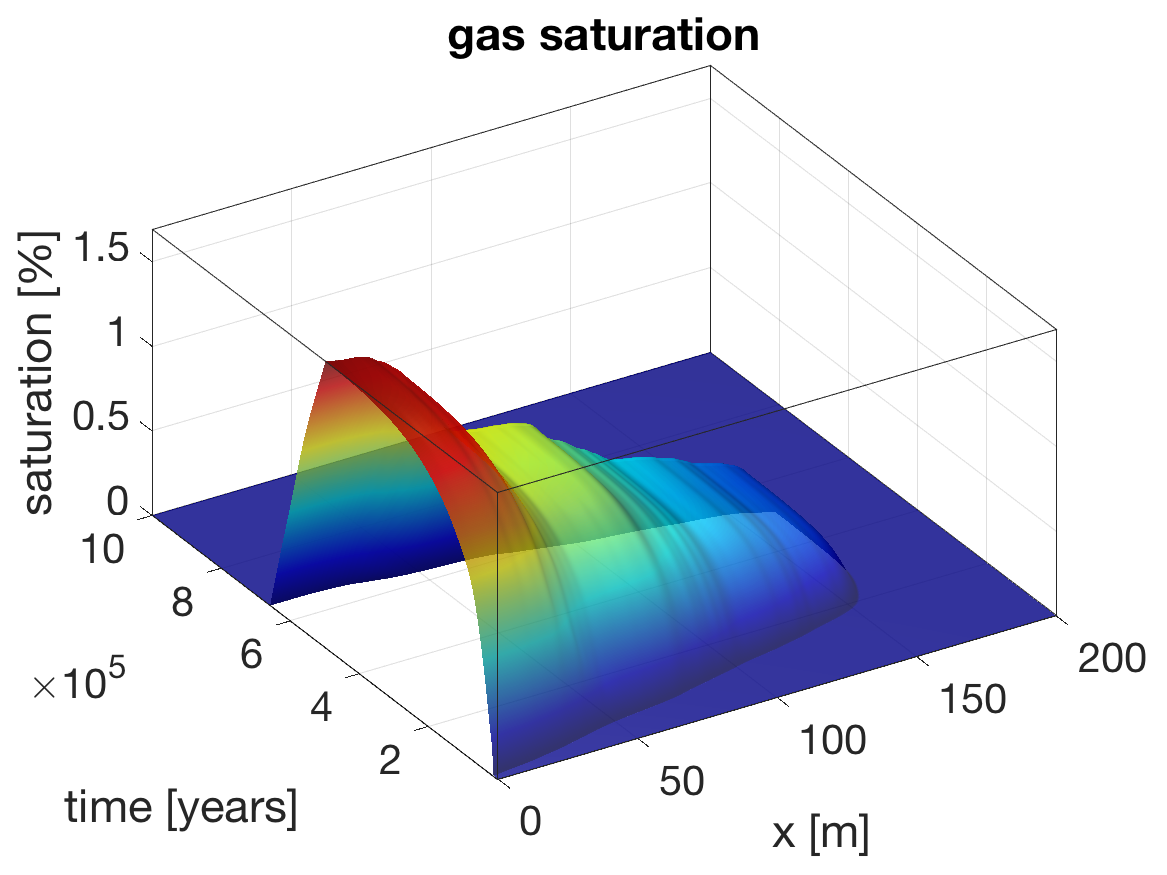
Figure 7: Space time evolution of gas saturation.

4 Spectral representations of random processes

4.1 Karhunen Loéve expansions

Here we discuss spectral representations of a function-valued output $f(s,{\mathchoice{\mbox{\boldmath$\displaystyle{\xi}$}}{\mbox{\boldmath$\textstyle{\xi}$}}{\mbox{\boldmath$\scriptstyle{\xi}$}}{\mbox{\boldmath$\scriptscriptstyle{\xi}$}}})$. We assume $f$ is a mean-square continuous random process. Such processes admit spectral representations, as given by a Karhunen Loéve expansion (KLE) Loeve77 ; Maitre10 :

$$f(s,{\mathchoice{\mbox{\boldmath$\displaystyle{\xi}$}}{\mbox{\boldmath$\textstyle{\xi}$}}{\mbox{\boldmath$\scriptstyle{\xi}$}}{\mbox{\boldmath$\scriptscriptstyle{\xi}$}}})=\bar{f}(s)+\sum_{i=1}^{\infty}\sqrt{\lambda_{i}}f_{i}({\mathchoice{\mbox{\boldmath$\displaystyle{\xi}$}}{\mbox{\boldmath$\textstyle{\xi}$}}{\mbox{\boldmath$\scriptstyle{\xi}$}}{\mbox{\boldmath$\scriptscriptstyle{\xi}$}}})\Phi_{i}(s).$$ (11)

Here $\bar{f}(s)$ is the mean of the process, $(\lambda_{i},\Phi_{i})$ are the eigenpairs of the covariance operator $\mathcal{C}_{\text{qoi}}$ of the process,

$$\mathcal{C}_{\text{qoi}}\Phi_{i}=\lambda_{i}\Phi_{i},\quad i=1,2,\ldots,$$ (12)

and $f_{i}({\mathchoice{\mbox{\boldmath$\displaystyle{\xi}$}}{\mbox{\boldmath$\textstyle{\xi}$}}{\mbox{\boldmath$\scriptstyle{\xi}$}}{\mbox{\boldmath$\scriptscriptstyle{\xi}$}}})$ are the KL modes,

$$f_{i}({\mathchoice{\mbox{\boldmath$\displaystyle{\xi}$}}{\mbox{\boldmath$\textstyle{\xi}$}}{\mbox{\boldmath$\scriptstyle{\xi}$}}{\mbox{\boldmath$\scriptscriptstyle{\xi}$}}})=\frac{1}{\sqrt{\lambda_{i}}}\int_{\mathscr{X}}\big{(}f(s,{\mathchoice{\mbox{\boldmath$\displaystyle{\xi}$}}{\mbox{\boldmath$\textstyle{\xi}$}}{\mbox{\boldmath$\scriptstyle{\xi}$}}{\mbox{\boldmath$\scriptscriptstyle{\xi}$}}})-\bar{f}(s)\big{)}\Phi_{i}(s)\,ds,\quad i=1,2,3,\ldots$$

An approximation $f_{{{{{N}_{\text{qoi}}}}\!}}(s,{\mathchoice{\mbox{\boldmath$\displaystyle{\xi}$}}{\mbox{\boldmath$\textstyle{\xi}$}}{\mbox{\boldmath$\scriptstyle{\xi}$}}{\mbox{\boldmath$\scriptscriptstyle{\xi}$}}})$ to $f(s,{\mathchoice{\mbox{\boldmath$\displaystyle{\xi}$}}{\mbox{\boldmath$\textstyle{\xi}$}}{\mbox{\boldmath$\scriptstyle{\xi}$}}{\mbox{\boldmath$\scriptscriptstyle{\xi}$}}})$ can be obtained by truncating (11) and retaining the first ${{N}_{\text{qoi}}}$ terms in the series. In many physical and biological models the eigenvalues of $\mathcal{C}_{\text{qoi}}$ decay rapidly. Consequently, such QoIs can be represented with sufficient accuracy by a truncated KLE with a small ${{N}_{\text{qoi}}}$. Such processes are referred to as “low-rank”.

We rely on Nyström’s method to compute the KLE Kress14 . This approach, as used in the present work, requires sample averaging to approximate the covariance kernel, because we do not in general have a closed-form expression for the output covariance operator. Typically, a modest number of QoI evaluations is sufficient for accurately estimating the dominant eigenpairs of the covariance operator $\mathcal{C}_{\text{qoi}}$. To determine a suitable value for the number ${{N}_{\text{qoi}}}$ of terms in a truncated KLE, we consider

$$r_{k}=\frac{\sum_{i=1}^{k}\lambda_{i}}{\sum_{i=1}^{\infty}\lambda_{i}}.$$ (13)

The quantity $r_{k}$ represents the fraction of the average variance of $f$ captured by the first $k$ eigenvalues. The steps for computing the truncated KLE of $f$ are included in Algorithm 1, which is adapted from AlexanderianReeseSmithEtAl18 .

Note that evaluating the truncated KLE of $f$ requires computing the KL modes, which in turn requires a model evaluation. To convert the truncated KLE into an efficient surrogate model for $f$, we need a cheap-to-evaluate representation for the KL modes. This approach is similar to the one taken by AlexanderianGremaudSmith20 ; LiIskandaraniLeHenaff16 , in which PCE surrogates are constructed for the modes of the related spectral representations. In section 5, we modify this approach by first reducing the dimension of the input parameter and then constructing the KL modes surrogates in the reduced uncertain parameter space.

4.2 Polynomial chaos expansions for $f_{i}({\mathchoice{\mbox{\boldmath$\displaystyle{\xi}$}}{\mbox{\boldmath$\textstyle{\xi}$}}{\mbox{\boldmath$\scriptstyle{\xi}$}}{\mbox{\boldmath$\scriptscriptstyle{\xi}$}}})$.

Recall, the polynomial chaos expansion of a square integrable function $g({\mathchoice{\mbox{\boldmath$\displaystyle{\xi}$}}{\mbox{\boldmath$\textstyle{\xi}$}}{\mbox{\boldmath$\scriptstyle{\xi}$}}{\mbox{\boldmath$\scriptscriptstyle{\xi}$}}})$ is a series approximation of the form

$$g({\mathchoice{\mbox{\boldmath$\displaystyle{\xi}$}}{\mbox{\boldmath$\textstyle{\xi}$}}{\mbox{\boldmath$\scriptstyle{\xi}$}}{\mbox{\boldmath$\scriptscriptstyle{\xi}$}}})\approx\sum_{k=0}^{{N}_{\text{PC}}}c_{k}{\Psi}_{k}({\mathchoice{\mbox{\boldmath$\displaystyle{\xi}$}}{\mbox{\boldmath$\textstyle{\xi}$}}{\mbox{\boldmath$\scriptstyle{\xi}$}}{\mbox{\boldmath$\scriptscriptstyle{\xi}$}}}),$$ (14)

where $\{{\Psi}_{k}\}_{k=0}^{{N}_{\text{PC}}}$ are a predetermined set of orthogonal polynomials, and $\{c_{k}\}_{k=0}^{{N}_{\text{PC}}}$ are the corresponding expansion coefficients Maitre10 . Following a total order truncation Maitre10 , ${N}_{\text{PC}}$ is given by

$${N}_{\text{PC}}+1=\frac{({N}_{\text{ord}}+{{N}_{\text{p}}})!}{{N}_{\text{ord}}!{{N}_{\text{p}}}!},$$

where ${N}_{\text{ord}}$ is the maximum total polynomial degree and ${{N}_{\text{p}}}$ is the dimension of $\textstyle{\xi}$. There are a variety of approaches for determining the expansion coefficients $\{c_{k}\}_{k=0}^{{N}_{\text{PC}}}$ including quadrature or regression based methods Maitre10 . For this application, we implement sparse linear regression Fajraoui17 ; Yan12 . In this method, the expansion coefficients are found by solving

$$\min_{{\mathchoice{\mbox{\boldmath$\displaystyle{c}$}}{\mbox{\boldmath$\textstyle{c}$}}{\mbox{\boldmath$\scriptstyle{c}$}}{\mbox{\boldmath$\scriptscriptstyle{c}$}}}\in\mathbb{R}^{{N}_{\text{PC}}}}\left\|{\mathchoice{\mbox{\boldmath$\displaystyle{\Lambda}$}}{\mbox{\boldmath$\textstyle{\Lambda}$}}{\mbox{\boldmath$\scriptstyle{\Lambda}$}}{\mbox{\boldmath$\scriptscriptstyle{\Lambda}$}}}{\mathchoice{\mbox{\boldmath$\displaystyle{c}$}}{\mbox{\boldmath$\textstyle{c}$}}{\mbox{\boldmath$\scriptstyle{c}$}}{\mbox{\boldmath$\scriptscriptstyle{c}$}}}-{\mathchoice{\mbox{\boldmath$\displaystyle{d}$}}{\mbox{\boldmath$\textstyle{d}$}}{\mbox{\boldmath$\scriptstyle{d}$}}{\mbox{\boldmath$\scriptscriptstyle{d}$}}}\right\|_{2}^{2},\quad\text{subject to }\sum_{k=0}^{{N}_{\text{PC}}}|c_{k}|\leq\tau,$$ (15)

where ${\mathchoice{\mbox{\boldmath$\displaystyle{\Lambda}$}}{\mbox{\boldmath$\textstyle{\Lambda}$}}{\mbox{\boldmath$\scriptstyle{\Lambda}$}}{\mbox{\boldmath$\scriptscriptstyle{\Lambda}$}}}\in\mathbb{R}^{{N}_{\text{s}}\times{N}_{\text{PC}}}$ is defined by $\Lambda_{ij}={\Psi}_{j}({\mathchoice{\mbox{\boldmath$\displaystyle{\xi}$}}{\mbox{\boldmath$\textstyle{\xi}$}}{\mbox{\boldmath$\scriptstyle{\xi}$}}{\mbox{\boldmath$\scriptscriptstyle{\xi}$}}}_{i})$,
${\mathchoice{\mbox{\boldmath$\displaystyle{d}$}}{\mbox{\boldmath$\textstyle{d}$}}{\mbox{\boldmath$\scriptstyle{d}$}}{\mbox{\boldmath$\scriptscriptstyle{d}$}}}=(g({\mathchoice{\mbox{\boldmath$\displaystyle{\xi}$}}{\mbox{\boldmath$\textstyle{\xi}$}}{\mbox{\boldmath$\scriptstyle{\xi}$}}{\mbox{\boldmath$\scriptscriptstyle{\xi}$}}}_{1}),g({\mathchoice{\mbox{\boldmath$\displaystyle{\xi}$}}{\mbox{\boldmath$\textstyle{\xi}$}}{\mbox{\boldmath$\scriptstyle{\xi}$}}{\mbox{\boldmath$\scriptscriptstyle{\xi}$}}}_{2}),\dots,g({\mathchoice{\mbox{\boldmath$\displaystyle{\xi}$}}{\mbox{\boldmath$\textstyle{\xi}$}}{\mbox{\boldmath$\scriptstyle{\xi}$}}{\mbox{\boldmath$\scriptscriptstyle{\xi}$}}}_{{N}_{\text{s}}}))^{\mkern-1.5mu\mathsf{T}}$ is a vector containing model evaluations, and $\tau$ is the sparsity control parameter. Determining ${N}_{\text{ord}}$ and $\tau$ may be done with trial and error or with a cross-validation process, as detailed in Section 6.

4.3 Bispectral surrogates

Earlier we broached the subject of utilizing PCEs to convert a truncated KLE into a surrogate model for $f$. Consider the truncated KLE of $f$,

$$f_{{{{{N}_{\text{qoi}}}}\!}}(s,{\mathchoice{\mbox{\boldmath$\displaystyle{\xi}$}}{\mbox{\boldmath$\textstyle{\xi}$}}{\mbox{\boldmath$\scriptstyle{\xi}$}}{\mbox{\boldmath$\scriptscriptstyle{\xi}$}}})=\bar{f}(s)+\sum_{i=1}^{{{N}_{\text{qoi}}}}\sqrt{\lambda_{i}}f_{i}({\mathchoice{\mbox{\boldmath$\displaystyle{\xi}$}}{\mbox{\boldmath$\textstyle{\xi}$}}{\mbox{\boldmath$\scriptstyle{\xi}$}}{\mbox{\boldmath$\scriptscriptstyle{\xi}$}}})\Phi_{i}(s).$$ (16)

By replacing the KL modes in (16) with PCEs we construct a surrogate model for $f$ of the form

$$f_{{{{{N}_{\text{qoi}}}}\!}}^{{\text{PC}}}(s,{\mathchoice{\mbox{\boldmath$\displaystyle{\xi}$}}{\mbox{\boldmath$\textstyle{\xi}$}}{\mbox{\boldmath$\scriptstyle{\xi}$}}{\mbox{\boldmath$\scriptscriptstyle{\xi}$}}})=\bar{f}(s)+\sum_{i=1}^{{{N}_{\text{qoi}}}}\sqrt{\lambda_{i}}f_{i}^{\text{PC}}({\mathchoice{\mbox{\boldmath$\displaystyle{\xi}$}}{\mbox{\boldmath$\textstyle{\xi}$}}{\mbox{\boldmath$\scriptstyle{\xi}$}}{\mbox{\boldmath$\scriptscriptstyle{\xi}$}}})\Phi_{i}(s),$$ (17)

where $f_{i}^{\text{PC}}({\mathchoice{\mbox{\boldmath$\displaystyle{\xi}$}}{\mbox{\boldmath$\textstyle{\xi}$}}{\mbox{\boldmath$\scriptstyle{\xi}$}}{\mbox{\boldmath$\scriptscriptstyle{\xi}$}}})$ is the PCE for $f_{i}({\mathchoice{\mbox{\boldmath$\displaystyle{\xi}$}}{\mbox{\boldmath$\textstyle{\xi}$}}{\mbox{\boldmath$\scriptstyle{\xi}$}}{\mbox{\boldmath$\scriptscriptstyle{\xi}$}}})$, $i=1,\ldots,{{N}_{\text{qoi}}}$. Once constructed, a bispectral surrogate can be used to characterize the statistical properties of the field QoI very efficiently.

To provide further insight, we also consider the approximation error for a bispectral surrogate. Let $\left\|\cdot\right\|$, represent the $L^{2}$ norm in the product space $\Theta\times\mathscr{X}$. The total error can be bounded as follows:

$$\left\|f-f_{{{{{N}_{\text{qoi}}}}\!}}^{{\text{PC}}}\right\|^{2} \leq 2\left\|f-f_{{{{{N}_{\text{qoi}}}}\!}}\right\|^{2}+2\left\|f_{{{{{N}_{\text{qoi}}}}\!}}-f_{{{{{N}_{\text{qoi}}}}\!}}^{{\text{PC}}}\right\|^{2}$$

$$=2\sum_{i={{N}_{\text{qoi}}}+1}^{\infty}\lambda_{i}$$

$$+\quad 2\sum_{i=1}^{{{N}_{\text{qoi}}}}\lambda_{i}\Big{[}\sum_{k=0}^{{N}_{\text{PC}}}(c_{i,k}-\hat{c}_{i,k})^{2}\left\|\Psi_{k}\right\|_{L^{2}(\Theta)}^{2}\Big{]}$$

$$+\quad 2\sum_{i=1}^{{{N}_{\text{qoi}}}}\lambda_{i}\Big{[}\sum_{j=1+{N}_{\text{PC}}}^{\infty}c_{i,j}^{2}\left\|\Psi_{j}\right\|_{L^{2}(\Theta)}^{2}\Big{]}.$$

See Appendix 8, for a derivation of this bound. The first term in the upper bound corresponds to KLE truncation error, the second term corresponds to error due to inexact PCE coefficients, and the third term corresponds to PCE truncation error.

Controlling the total error involves a balance between computational cost, accuracy requirements, and the properties of the process. The KLE truncation error gets smaller as ${{N}_{\text{qoi}}}$ increases. However, increasing the number of terms in the KLE increases the number of eigenpairs that need accurate approximations. Also, a larger ${{N}_{\text{qoi}}}$ results in more KL modes, each of which requires a sufficiently accurate PCE. Similarly, the PCE error can be minimized by increasing the maximum polynomial degree, ${N}_{\text{ord}}$. However, this increases the total number of coefficients, which increases the number of unknowns in (14), resulting in increased computational cost.

The function-valued QoIs in the present work are low-rank processes with a high-dimensional input parameter. Therefore, a modest ${{N}_{\text{qoi}}}$ will give a sufficiently small KLE truncation error. However, for large ${{N}_{\text{p}}}$, estimating the PCE coefficients for each KL mode with sufficient accuracy can become computationally expensive. Our approach for addressing this challenge is presented in the next section.

Algorithm 1 Computing the truncated KLE of $f$

.

0:  Quadrature nodes $s_{k}$ and weights $w_{k}$, $k=1,\ldots,m$; Function evaluations $y_{k}^{j}=f(s_{k},{\mathchoice{\mbox{\boldmath$\displaystyle{\xi}$}}{\mbox{\boldmath$\textstyle{\xi}$}}{\mbox{\boldmath$\scriptstyle{\xi}$}}{\mbox{\boldmath$\scriptscriptstyle{\xi}$}}}_{j})$, $k=1,\ldots,m$, $j=1,\ldots,{N}_{\text{s}}$; $r_{k}$ tolerance $0<tol<1$.

0:  Eigenpairs $\left(\lambda_{i},{\mathchoice{\mbox{\boldmath$\displaystyle{\Phi}$}}{\mbox{\boldmath$\textstyle{\Phi}$}}{\mbox{\boldmath$\scriptstyle{\Phi}$}}{\mbox{\boldmath$\scriptscriptstyle{\Phi}$}}}_{i}\right)$ of the output covariance operator, and KL modes evaluations $f_{i}({\mathchoice{\mbox{\boldmath$\displaystyle{\xi_{j}}$}}{\mbox{\boldmath$\textstyle{\xi_{j}}$}}{\mbox{\boldmath$\scriptstyle{\xi_{j}}$}}{\mbox{\boldmath$\scriptscriptstyle{\xi_{j}}$}}})$, $j=1,\ldots,{N}_{\text{s}}$, $i=1,\ldots{{N}_{\text{qoi}}}$.

1:  Compute mean $M_{k}=\frac{1}{{N}_{\text{s}}}\sum_{j=1}^{{N}_{\text{s}}}y_{k}^{j}$, $k=1,\ldots m$.

2:  Center process $f_{k}^{c}(s_{k},{\mathchoice{\mbox{\boldmath$\displaystyle{\xi}$}}{\mbox{\boldmath$\textstyle{\xi}$}}{\mbox{\boldmath$\scriptstyle{\xi}$}}{\mbox{\boldmath$\scriptscriptstyle{\xi}$}}}^{j})=y_{k}^{j}-M_{k}$, $k=1,\ldots,m$.

3:  Compute covariance matrix $\mathbf{{C}}$.$\mathbf{{C}}_{kl}=\frac{1}{{N}_{\text{s}}-1}\sum_{j=1}^{{N}_{\text{s}}}f_{k}^{c}(s_{k},{\mathchoice{\mbox{\boldmath$\displaystyle{\xi}$}}{\mbox{\boldmath$\textstyle{\xi}$}}{\mbox{\boldmath$\scriptstyle{\xi}$}}{\mbox{\boldmath$\scriptscriptstyle{\xi}$}}}_{j})f_{l}^{c}(s_{l},{\mathchoice{\mbox{\boldmath$\displaystyle{\xi}$}}{\mbox{\boldmath$\textstyle{\xi}$}}{\mbox{\boldmath$\scriptstyle{\xi}$}}{\mbox{\boldmath$\scriptscriptstyle{\xi}$}}}_{j})$, $k,l=1,\ldots m$.

4:  Let $\mathbf{{W}}=\text{diag}(w_{1},w_{2},\ldots w_{m})$ solve:$\mathbf{{W}}^{1/2}\mathbf{{C}}\mathbf{{W}}^{1/2}{\mathchoice{\mbox{\boldmath$\displaystyle{v}$}}{\mbox{\boldmath$\textstyle{v}$}}{\mbox{\boldmath$\scriptstyle{v}$}}{\mbox{\boldmath$\scriptscriptstyle{v}$}}}_{k}=\lambda_{k}{\mathchoice{\mbox{\boldmath$\displaystyle{v}$}}{\mbox{\boldmath$\textstyle{v}$}}{\mbox{\boldmath$\scriptstyle{v}$}}{\mbox{\boldmath$\scriptscriptstyle{v}$}}}_{k}$, $k=1,\ldots,m$.

5:  Determine ${{N}_{\text{qoi}}}$.

6:  for $k=1,\ldots m$ do

7:     Compute $r_{k}=\frac{\sum_{l=1}^{k}\lambda_{l}}{\sum_{l=1}^{m}\lambda_{l}}$.

8:     if $r_{k}>tol$ then

9:        ${{N}_{\text{qoi}}}=k$; BREAK

10:     end if

11:  end for

12:  Compute ${\mathchoice{\mbox{\boldmath$\displaystyle{\Phi}$}}{\mbox{\boldmath$\textstyle{\Phi}$}}{\mbox{\boldmath$\scriptstyle{\Phi}$}}{\mbox{\boldmath$\scriptscriptstyle{\Phi}$}}}_{k}=\mathbf{{W}}^{-1/2}{\mathchoice{\mbox{\boldmath$\displaystyle{v}$}}{\mbox{\boldmath$\textstyle{v}$}}{\mbox{\boldmath$\scriptstyle{v}$}}{\mbox{\boldmath$\scriptscriptstyle{v}$}}}_{k}$, $k=1,\ldots,{{N}_{\text{qoi}}}$.

13:  Compute KL modes.$f_{i}({\mathchoice{\mbox{\boldmath$\displaystyle{\xi}$}}{\mbox{\boldmath$\textstyle{\xi}$}}{\mbox{\boldmath$\scriptstyle{\xi}$}}{\mbox{\boldmath$\scriptscriptstyle{\xi}$}}}_{j})=\frac{1}{\sqrt{\lambda_{i}}}\sum_{k=1}^{m}w_{k}f_{k}^{c}(s_{k},{\mathchoice{\mbox{\boldmath$\displaystyle{\xi}$}}{\mbox{\boldmath$\textstyle{\xi}$}}{\mbox{\boldmath$\scriptstyle{\xi}$}}{\mbox{\boldmath$\scriptscriptstyle{\xi}$}}}_{j}){\mathchoice{\mbox{\boldmath$\displaystyle{\Phi}$}}{\mbox{\boldmath$\textstyle{\Phi}$}}{\mbox{\boldmath$\scriptstyle{\Phi}$}}{\mbox{\boldmath$\scriptscriptstyle{\Phi}$}}}_{i}(s_{k})$, $i=1,\ldots,{{N}_{\text{qoi}}}$, $j=1,\ldots,{N}_{\text{s}}$.

14:  Compute $f_{{{{{N}_{\text{qoi}}}}\!}}(s,{\mathchoice{\mbox{\boldmath$\displaystyle{\xi}$}}{\mbox{\boldmath$\textstyle{\xi}$}}{\mbox{\boldmath$\scriptstyle{\xi}$}}{\mbox{\boldmath$\scriptscriptstyle{\xi}$}}}_{j})=\sum_{k=1}^{{{N}_{\text{qoi}}}}\sqrt{\lambda_{k}}f_{i}({\mathchoice{\mbox{\boldmath$\displaystyle{\xi}$}}{\mbox{\boldmath$\textstyle{\xi}$}}{\mbox{\boldmath$\scriptstyle{\xi}$}}{\mbox{\boldmath$\scriptscriptstyle{\xi}$}}}_{j}){\mathchoice{\mbox{\boldmath$\displaystyle{\Phi}$}}{\mbox{\boldmath$\textstyle{\Phi}$}}{\mbox{\boldmath$\scriptstyle{\Phi}$}}{\mbox{\boldmath$\scriptscriptstyle{\Phi}$}}}_{k}(s)$.

5 Method

In this section, we present our approach for reducing the dimensionality of the random vector ${\mathchoice{\mbox{\boldmath$\displaystyle{\xi}$}}{\mbox{\boldmath$\textstyle{\xi}$}}{\mbox{\boldmath$\scriptstyle{\xi}$}}{\mbox{\boldmath$\scriptscriptstyle{\xi}$}}}=[\begin{matrix}\xi_{1}&\xi_{2}&\ldots&\xi_{{N}_{\text{p}}}\end{matrix}]^{\mkern-1.5mu\mathsf{T}}$ and constructing a cheap-to-compute bispectral surrogate for function-valued QoIs under study. We begin by describing a screening procedure for input dimension reduction in Section 5.1. Then, we discuss our surrogate modeling approach that utilizes a truncated KLE of the output (Section 4.1) along with generalized PCEs for the output KL modes (Section 5.2). We also show how the surrogate model can be used to efficiently compute the correlation function of the output, as well as cross-correlation of two function-valued QoIs.

5.1 Parameter screening

Consider a function-valued QoI $f(s,{\mathchoice{\mbox{\boldmath$\displaystyle{\xi}$}}{\mbox{\boldmath$\textstyle{\xi}$}}{\mbox{\boldmath$\scriptstyle{\xi}$}}{\mbox{\boldmath$\scriptscriptstyle{\xi}$}}}):\mathscr{X}\times\Theta\to\mathbb{R}$, where $\Theta\subseteq\mathbb{R}^{{N}_{\text{p}}}$ is the sample space of the uncertain parameters and $\mathscr{X}\subseteq\mathbb{R}^{d}$ is a compact set. The set $\mathscr{X}$ can be either a time interval, in which case $d=1$, or a spatial region, in which case $d\in\{1,2,3\}$. Here we consider the case of $d=1$, as it applies to our application problem, but the procedure below can be generalized to the case of $d\in\{2,3\}$ in a straightforward manner.

Parameter screening can be done using functional derivative-based global sensitivity measures (DGSMs) given by CleavesAlexanderianGuyEtAl19 :

$$\mathbb{N}_{j}(f)=\int_{\mathscr{X}}\int_{\Theta}\left(\frac{\partial f(s,{\mathchoice{\mbox{\boldmath$\displaystyle{\xi}$}}{\mbox{\boldmath$\textstyle{\xi}$}}{\mbox{\boldmath$\scriptstyle{\xi}$}}{\mbox{\boldmath$\scriptscriptstyle{\xi}$}}})}{\partial\xi_{j}}\right)^{2}\,\!\upmu(d{\mathchoice{\mbox{\boldmath$\displaystyle{\xi}$}}{\mbox{\boldmath$\textstyle{\xi}$}}{\mbox{\boldmath$\scriptstyle{\xi}$}}{\mbox{\boldmath$\scriptscriptstyle{\xi}$}}})\,ds,\quad j=1,\ldots,{{N}_{\text{p}}},$$ (18)

where $\!\upmu$ is the law of the parameter vector $\textstyle{\xi}$. These DGSMs can be used to screen for “unimportant” inputs, which can be fixed at their respective nominal values. These functional DGSMs, however, require gradient evaluations. For complex models with high-dimensional parameters, such as the one considered in the present work, gradient computation is challenging. While adjoint-based gradient computation can overcome this, adjoint solvers are not always available for complex flow solvers and implementing them may be infeasible. Here we derive a screening indices based on ideas from active subspace methods Constantine15 and activity scores ConstantineDiaz17 that approximate the functional DGSMs and circumvent gradient computation.

Let us briefly recall the concept of the active subspace and activity scores ConstantineDiaz17 . Fix $s\in\mathscr{X}$ and let $(\lambda_{k},{\mathchoice{\mbox{\boldmath$\displaystyle{u}$}}{\mbox{\boldmath$\textstyle{u}$}}{\mbox{\boldmath$\scriptstyle{u}$}}{\mbox{\boldmath$\scriptscriptstyle{u}$}}}_{k})$, $k=1,\ldots,{{N}_{\text{p}}}$ be the eigenpairs of the matrix

$$\mathbf{{G}}=\int_{\Theta}[\nabla f(s,{\mathchoice{\mbox{\boldmath$\displaystyle{\xi}$}}{\mbox{\boldmath$\textstyle{\xi}$}}{\mbox{\boldmath$\scriptstyle{\xi}$}}{\mbox{\boldmath$\scriptscriptstyle{\xi}$}}})][\nabla f(s,{\mathchoice{\mbox{\boldmath$\displaystyle{\xi}$}}{\mbox{\boldmath$\textstyle{\xi}$}}{\mbox{\boldmath$\scriptstyle{\xi}$}}{\mbox{\boldmath$\scriptscriptstyle{\xi}$}}})]^{\mkern-1.5mu\mathsf{T}}\,\!\upmu(d{\mathchoice{\mbox{\boldmath$\displaystyle{\xi}$}}{\mbox{\boldmath$\textstyle{\xi}$}}{\mbox{\boldmath$\scriptstyle{\xi}$}}{\mbox{\boldmath$\scriptscriptstyle{\xi}$}}}),$$ (19)

where we assume the eigenvalues are sorted in descending order. In many cases there exists an $M$ such that $\lambda_{M}\ll\lambda_{M+1}$, representing a gap in the eigenvalues. The active subspace corresponds to the subspace spanned by eigenvectors $\{{\mathchoice{\mbox{\boldmath$\displaystyle{u}$}}{\mbox{\boldmath$\textstyle{u}$}}{\mbox{\boldmath$\scriptstyle{u}$}}{\mbox{\boldmath$\scriptscriptstyle{u}$}}}_{k}\}_{k=1}^{M}$; this subspace captures the directions in the uncertain parameter space along which the QoI varies most. The case of a one-dimensional active subspace is surprisingly common Constantine15 . The activity scores ConstantineDiaz17 utilize the active subspace structure to provide approximate screening indices, given by

$$\alpha_{j}[f(s,\cdot);M]=\sum_{k=1}^{M}\lambda_{k}\langle{{\mathchoice{\mbox{\boldmath$\displaystyle{e}$}}{\mbox{\boldmath$\textstyle{e}$}}{\mbox{\boldmath$\scriptstyle{e}$}}{\mbox{\boldmath$\scriptscriptstyle{e}$}}}_{j}},{{\mathchoice{\mbox{\boldmath$\displaystyle{u}$}}{\mbox{\boldmath$\textstyle{u}$}}{\mbox{\boldmath$\scriptstyle{u}$}}{\mbox{\boldmath$\scriptscriptstyle{u}$}}}_{k}}\rangle^{2},\quad j=1,\ldots,{{N}_{\text{p}}},\quad M\leq{{N}_{\text{p}}},$$ (20)

where $\langle{\cdot},{\cdot}\rangle$ denotes the Euclidean inner product and ${\mathchoice{\mbox{\boldmath$\displaystyle{e}$}}{\mbox{\boldmath$\textstyle{e}$}}{\mbox{\boldmath$\scriptstyle{e}$}}{\mbox{\boldmath$\scriptscriptstyle{e}$}}}_{j}$ is the $j$th coordinate vector in $\mathbb{R}^{{N}_{\text{p}}}$. One can use the activity scores to approximate functional DGSMs according to

$$\int_{\mathscr{X}}\alpha_{j}[f(s,\cdot);M]\,ds,\quad j=1,\ldots,{{N}_{\text{p}}}.$$

Note that with $M={{N}_{\text{p}}}$, we recover the exact DGSMs ConstantineDiaz17 . Computing the activity scores still requires gradient computation, as seen in the definition of the matrix $\mathbf{{G}}$ in (19). For cases where full model gradients are unavailable, we propose use of suitable and cheap-to-compute surrogate models for the purpose of computing the activity scores. One possibility is the use of global linear models as done in Constantine15 , for the case of scalar QoIs. Building on this idea, we use a global linear model for $f(s,{\mathchoice{\mbox{\boldmath$\displaystyle{\xi}$}}{\mbox{\boldmath$\textstyle{\xi}$}}{\mbox{\boldmath$\scriptstyle{\xi}$}}{\mbox{\boldmath$\scriptscriptstyle{\xi}$}}})$, use the gradient of the linear model to approximate the matrix $\mathbf{{G}}$, and define screening indices for function-valued QoIs. Specifically, we construct a global linear approximation $\tilde{f}$ for the QoI

$$\tilde{f}(s,{\mathchoice{\mbox{\boldmath$\displaystyle{\xi}$}}{\mbox{\boldmath$\textstyle{\xi}$}}{\mbox{\boldmath$\scriptstyle{\xi}$}}{\mbox{\boldmath$\scriptscriptstyle{\xi}$}}})=b_{0}(s)+\sum_{j=1}^{{N}_{\text{p}}}b_{j}(s)\xi_{j}.$$ (21)

Next, we use the activity scores for $\tilde{f}$ as a “surrogate” for the scores of $f$. Note that $\nabla\tilde{f}(s,{\mathchoice{\mbox{\boldmath$\displaystyle{\xi}$}}{\mbox{\boldmath$\textstyle{\xi}$}}{\mbox{\boldmath$\scriptstyle{\xi}$}}{\mbox{\boldmath$\scriptscriptstyle{\xi}$}}})={\mathchoice{\mbox{\boldmath$\displaystyle{b}$}}{\mbox{\boldmath$\textstyle{b}$}}{\mbox{\boldmath$\scriptstyle{b}$}}{\mbox{\boldmath$\scriptscriptstyle{b}$}}}(s)$, where ${\mathchoice{\mbox{\boldmath$\displaystyle{b}$}}{\mbox{\boldmath$\textstyle{b}$}}{\mbox{\boldmath$\scriptstyle{b}$}}{\mbox{\boldmath$\scriptscriptstyle{b}$}}}(s)=[\begin{matrix}b_{1}(t)&b_{2}(t)&\cdots&b_{{N}_{\text{p}}}(t)\end{matrix}]^{\mkern-1.5mu\mathsf{T}}$. The matrix $\mathbf{{G}}(s)$ in (19), using $\tilde{f}$ in place of $f$ then simplifies to $\mathbf{{G}}(s)={\mathchoice{\mbox{\boldmath$\displaystyle{b}$}}{\mbox{\boldmath$\textstyle{b}$}}{\mbox{\boldmath$\scriptstyle{b}$}}{\mbox{\boldmath$\scriptscriptstyle{b}$}}}(s){\mathchoice{\mbox{\boldmath$\displaystyle{b}$}}{\mbox{\boldmath$\textstyle{b}$}}{\mbox{\boldmath$\scriptstyle{b}$}}{\mbox{\boldmath$\scriptscriptstyle{b}$}}}(s)^{\mkern-1.5mu\mathsf{T}}$. This rank one matrix can be written as

$$\mathbf{{G}}(s)=\lambda{\mathchoice{\mbox{\boldmath$\displaystyle{u}$}}{\mbox{\boldmath$\textstyle{u}$}}{\mbox{\boldmath$\scriptstyle{u}$}}{\mbox{\boldmath$\scriptscriptstyle{u}$}}}(s){\mathchoice{\mbox{\boldmath$\displaystyle{u}$}}{\mbox{\boldmath$\textstyle{u}$}}{\mbox{\boldmath$\scriptstyle{u}$}}{\mbox{\boldmath$\scriptscriptstyle{u}$}}}(s)^{\mkern-1.5mu\mathsf{T}},$$

where $\lambda=\left\|{\mathchoice{\mbox{\boldmath$\displaystyle{b}$}}{\mbox{\boldmath$\textstyle{b}$}}{\mbox{\boldmath$\scriptstyle{b}$}}{\mbox{\boldmath$\scriptscriptstyle{b}$}}}(s)\right\|_{2}^{2}$, and ${\mathchoice{\mbox{\boldmath$\displaystyle{u}$}}{\mbox{\boldmath$\textstyle{u}$}}{\mbox{\boldmath$\scriptstyle{u}$}}{\mbox{\boldmath$\scriptscriptstyle{u}$}}}(s)={\mathchoice{\mbox{\boldmath$\displaystyle{b}$}}{\mbox{\boldmath$\textstyle{b}$}}{\mbox{\boldmath$\scriptstyle{b}$}}{\mbox{\boldmath$\scriptscriptstyle{b}$}}}(s)/\left\|{\mathchoice{\mbox{\boldmath$\displaystyle{b}$}}{\mbox{\boldmath$\textstyle{b}$}}{\mbox{\boldmath$\scriptstyle{b}$}}{\mbox{\boldmath$\scriptscriptstyle{b}$}}}(s)\right\|_{2}$. (Here $\left\|\cdot\right\|_{2}$ denotes the Euclidean vector norm.) Hence, the corresponding active subspace for $\tilde{f}$ is 1-dimensional resulting in activity scores

$$\tilde{\alpha}_{j}(s)=b_{j}^{2}(s),\quad j=1,\ldots,{{N}_{\text{p}}}.$$

This gives rise to the following approximate functional DGSMs:

$$\tilde{\mathbb{N}}_{j}(f):=\int_{\mathscr{X}}b^{2}_{j}(s)\,ds.$$

This relationship motivates the following normalized screening indices

$$\mathfrak{s}_{j}=\frac{\tilde{\mathbb{N}}_{j}(f)}{\sum_{l=1}^{{N}_{\text{p}}}\tilde{\mathbb{N}}_{l}(f)},\quad j=1,\ldots,{{N}_{\text{p}}}.$$ (22)

Henceforth, we refer to $\mathfrak{s}_{j}$ as the screening index of $f$ with respect to parameters $\xi_{j}$.

The purpose of the screening indices $\mathfrak{s}_{j}$ is to inform input parameter dimension reduction. Let $K_{r}$ be an ordered index set with cardinality ${{n}_{\text{p}}}<{{N}_{\text{p}}}$, corresponding to parameters with a screening index above some tolerance $tol\in(0,1)$. We denote the reduced input parameter vectors ${\mathchoice{\mbox{\boldmath$\displaystyle{\xi}$}}{\mbox{\boldmath$\textstyle{\xi}$}}{\mbox{\boldmath$\scriptstyle{\xi}$}}{\mbox{\boldmath$\scriptscriptstyle{\xi}$}}}^{r}$, where each component $\xi_{i}^{r}$, $i=1,\ldots,{{n}_{\text{p}}}$ corresponds to the $i$th element of $K_{r}$.

Next, we discuss the computation of the global linear model for $f$. This is done by computing a linear model at each point $s\in\mathscr{X}$, which can be done efficiently using linear regression. Recall that $\mathscr{X}$ is assumed to be a (compact) subset of $\mathbb{R}$ (i.e., in one space dimension). Specifically, we assume $\mathscr{X}=[s_{0},s_{F}]$. We discretize $\mathscr{X}$ using a grid

$$s_{0}=s_{1}<s_{2}<s_{3}<\cdots<s_{m}=s_{F}.$$

Denote $\bar{{\mathchoice{\mbox{\boldmath$\displaystyle{b}$}}{\mbox{\boldmath$\textstyle{b}$}}{\mbox{\boldmath$\scriptstyle{b}$}}{\mbox{\boldmath$\scriptscriptstyle{b}$}}}}(s)=[\begin{matrix}b_{0}(s)&b_{1}(s)&b_{2}(s)&\cdots&b_{{{N}_{\text{p}}}}(s)\end{matrix}]^{\mkern-1.5mu\mathsf{T}}$, with $b_{j}$, $j=0,\ldots,{{N}_{\text{p}}}$ as in (21). We require a set of model evaluations,

$$y_{k}^{i}=f(s_{k},{\mathchoice{\mbox{\boldmath$\displaystyle{\xi}$}}{\mbox{\boldmath$\textstyle{\xi}$}}{\mbox{\boldmath$\scriptstyle{\xi}$}}{\mbox{\boldmath$\scriptscriptstyle{\xi}$}}}_{i}),\quad i=1,\ldots,{N}_{\text{s}}.$$

The number of samples required depends on computational budget as well as the application problem under study. We show in our numerical results that a modest ${N}_{\text{s}}$ is adequate for the proposed approach, and the application problem considered herein.

Let ${\mathchoice{\mbox{\boldmath$\displaystyle{y}$}}{\mbox{\boldmath$\textstyle{y}$}}{\mbox{\boldmath$\scriptstyle{y}$}}{\mbox{\boldmath$\scriptscriptstyle{y}$}}}_{k}=[\begin{matrix}y_{k}^{1}&y_{k}^{2}&\cdots&y_{k}^{{N}_{\text{s}}}\end{matrix}]^{\mkern-1.5mu\mathsf{T}}\in\mathbb{R}^{{N}_{\text{s}}}$, and define the matrix

$$\mathbf{{A}}=\begin{bmatrix}1&{\mathchoice{\mbox{\boldmath$\displaystyle{\xi}$}}{\mbox{\boldmath$\textstyle{\xi}$}}{\mbox{\boldmath$\scriptstyle{\xi}$}}{\mbox{\boldmath$\scriptscriptstyle{\xi}$}}}_{1}^{\mkern-1.5mu\mathsf{T}}\\ 1&{\mathchoice{\mbox{\boldmath$\displaystyle{\xi}$}}{\mbox{\boldmath$\textstyle{\xi}$}}{\mbox{\boldmath$\scriptstyle{\xi}$}}{\mbox{\boldmath$\scriptscriptstyle{\xi}$}}}_{2}^{\mkern-1.5mu\mathsf{T}}\\ 1&{\mathchoice{\mbox{\boldmath$\displaystyle{\xi}$}}{\mbox{\boldmath$\textstyle{\xi}$}}{\mbox{\boldmath$\scriptstyle{\xi}$}}{\mbox{\boldmath$\scriptscriptstyle{\xi}$}}}_{3}^{\mkern-1.5mu\mathsf{T}}\\ \vdots&\vdots\\ 1&{\mathchoice{\mbox{\boldmath$\displaystyle{\xi}$}}{\mbox{\boldmath$\textstyle{\xi}$}}{\mbox{\boldmath$\scriptstyle{\xi}$}}{\mbox{\boldmath$\scriptscriptstyle{\xi}$}}}_{{N}_{\text{s}}}^{\mkern-1.5mu\mathsf{T}}\end{bmatrix}.$$ (23)

The vectors $\bar{{\mathchoice{\mbox{\boldmath$\displaystyle{b}$}}{\mbox{\boldmath$\textstyle{b}$}}{\mbox{\boldmath$\scriptstyle{b}$}}{\mbox{\boldmath$\scriptscriptstyle{b}$}}}}(s_{k})$ can be computed numerically by solving linear least squares problems

$$\bar{{\mathchoice{\mbox{\boldmath$\displaystyle{b}$}}{\mbox{\boldmath$\textstyle{b}$}}{\mbox{\boldmath$\scriptstyle{b}$}}{\mbox{\boldmath$\scriptscriptstyle{b}$}}}}(s_{k})=\operatorname*{arg\,min}_{{\mathchoice{\mbox{\boldmath$\displaystyle{b}$}}{\mbox{\boldmath$\textstyle{b}$}}{\mbox{\boldmath$\scriptstyle{b}$}}{\mbox{\boldmath$\scriptscriptstyle{b}$}}}\in\mathbb{R}^{{N}_{\text{s}}+1}}\left\|\mathbf{{A}}{\mathchoice{\mbox{\boldmath$\displaystyle{b}$}}{\mbox{\boldmath$\textstyle{b}$}}{\mbox{\boldmath$\scriptstyle{b}$}}{\mbox{\boldmath$\scriptscriptstyle{b}$}}}-{\mathchoice{\mbox{\boldmath$\displaystyle{y}$}}{\mbox{\boldmath$\textstyle{y}$}}{\mbox{\boldmath$\scriptstyle{y}$}}{\mbox{\boldmath$\scriptscriptstyle{y}$}}}_{k}\right\|_{2}^{2},$$ (24)

for $k=1,\ldots,m$. Note that here we assume $\mathbf{{A}}$ has full column rank and we are in the overdetermined case, i.e. ${N}_{\text{s}}>{{N}_{\text{p}}}+1$. Under these assumptions, the QR factorization $\mathbf{{A}}=\mathbf{{Q}}\mathbf{{R}}$ may be used to solve the linear regression problem in (24) by

$$\bar{{\mathchoice{\mbox{\boldmath$\displaystyle{b}$}}{\mbox{\boldmath$\textstyle{b}$}}{\mbox{\boldmath$\scriptstyle{b}$}}{\mbox{\boldmath$\scriptscriptstyle{b}$}}}}(s_{k})=\mathbf{{R}}^{-1}\mathbf{{Q}}^{\mkern-1.5mu\mathsf{T}}{\mathchoice{\mbox{\boldmath$\displaystyle{y}$}}{\mbox{\boldmath$\textstyle{y}$}}{\mbox{\boldmath$\scriptstyle{y}$}}{\mbox{\boldmath$\scriptscriptstyle{y}$}}}_{k}.$$

Then, for each $k=1,\ldots,m$, the cost of computing ${\mathchoice{\mbox{\boldmath$\displaystyle{b}$}}{\mbox{\boldmath$\textstyle{b}$}}{\mbox{\boldmath$\scriptstyle{b}$}}{\mbox{\boldmath$\scriptscriptstyle{b}$}}}_{k}$ is one matrix-vector product with $\mathbf{{Q}}^{\mkern-1.5mu\mathsf{T}}$ and one triangular solve. The procedure for computing the global linear model is summarized in Algorithm 2. In the case where the dimension of $\textstyle{\xi}$ is larger than the number of available function evaluations, i.e. ${N}_{\text{s}}<{{N}_{\text{p}}}+1$, other methods for solving the linear regression in Equation (24), e.g. using SVD, can be used.

Note that when using a global linear model for the approximating function $\tilde{f}$, the screening indices (22) coincide with the normalized functional DGSMs of $\tilde{f}$,

$$\mathfrak{s}_{j}=\frac{\mathbb{N}_{j}(\tilde{f})}{\sum_{i=1}^{{N}_{\text{p}}}\mathbb{N}_{i}(\tilde{f})},$$

with $\mathbb{N}_{j}$ is as in (18). Additionally, since we have independent standard normal input parameters the screening indices are equal to the function-valued Sobol’ indices GamboaJanonKlein14 ; AlexanderianGremaudSmith20 of $\tilde{f}$, as well as the square root of the standard regression coefficients Helton93 ; ConstantineDiaz17 for $f$. In general, the relations across these sensitivity measures will not hold for alternative choices of $\tilde{f}$ or input parameter distributions.

We emphasize that, while simplifications occur when a global linear model is used, the proposed screening approach, i.e., computing activity scores of the $\tilde{f}$, is intended to be flexible and adjustable to alternative modeling approaches for $\tilde{f}$. Furthermore, the proposed screening method is not constrained by the assumption of independent parameters and can be used for the case of dependent inputs. The only requirements of the proposed screening method are that $\tilde{f}$ be cheap to compute and adequately approximate the full model for the purposes of parameter screening.

Algorithm 2 Computing the screening indices $\mathfrak{s}_{j}$, $j=1,\ldots,{{N}_{\text{p}}}$: the overdetermined case.

0:  Quadrature nodes $s_{k}$ and weights $w_{k}$, $k=1,\ldots,m$. Function evaluations $y_{k}^{i}=f(s_{k},{\mathchoice{\mbox{\boldmath$\displaystyle{\xi}$}}{\mbox{\boldmath$\textstyle{\xi}$}}{\mbox{\boldmath$\scriptstyle{\xi}$}}{\mbox{\boldmath$\scriptscriptstyle{\xi}$}}}_{i})$, $i=1,\ldots,{N}_{\text{s}}$, $k=1,\ldots,m$;

0:  Sensitivity measures $\mathfrak{s}_{j}$, $j=1,\ldots,{{N}_{\text{p}}}$.

1:  Form the matrix $\mathbf{{A}}$ in (23) and compute its QR factorization, $\mathbf{{A}}=\mathbf{{Q}}\mathbf{{R}}$.

2:  for $k=1$ to $m$ do

3:     Compute ${\mathchoice{\mbox{\boldmath$\displaystyle{z}$}}{\mbox{\boldmath$\textstyle{z}$}}{\mbox{\boldmath$\scriptstyle{z}$}}{\mbox{\boldmath$\scriptscriptstyle{z}$}}}_{k}=\mathbf{{Q}}^{\mkern-1.5mu\mathsf{T}}{\mathchoice{\mbox{\boldmath$\displaystyle{y}$}}{\mbox{\boldmath$\textstyle{y}$}}{\mbox{\boldmath$\scriptstyle{y}$}}{\mbox{\boldmath$\scriptscriptstyle{y}$}}}_{k}$.

4:     Solve $\mathbf{{R}}\bar{{\mathchoice{\mbox{\boldmath$\displaystyle{b}$}}{\mbox{\boldmath$\textstyle{b}$}}{\mbox{\boldmath$\scriptstyle{b}$}}{\mbox{\boldmath$\scriptscriptstyle{b}$}}}}(s_{k})={\mathchoice{\mbox{\boldmath$\displaystyle{z}$}}{\mbox{\boldmath$\textstyle{z}$}}{\mbox{\boldmath$\scriptstyle{z}$}}{\mbox{\boldmath$\scriptscriptstyle{z}$}}}_{k}$.

5:  end for

6:  for $j=1$ to ${{N}_{\text{p}}}$ do

7:     Compute $\tilde{\mathbb{N}}_{j}=\sum_{k=1}^{{N}_{\text{p}}}w_{k}b_{j}(s_{k})^{2}$.

8:  end for

9:  for $j=1$ to ${{N}_{\text{p}}}$ do

10:     Compute $\mathfrak{s}_{j}=\tilde{\mathbb{N}}_{j}/(\sum_{k}\tilde{\mathbb{N}}_{k})$.

11:  end for

5.2 Polynomial Chaos surrogates for KL modes

To form a surrogate model, we construct a PC surrogate $f_{i}^{\text{PC}}({\mathchoice{\mbox{\boldmath$\displaystyle{\xi}$}}{\mbox{\boldmath$\textstyle{\xi}$}}{\mbox{\boldmath$\scriptstyle{\xi}$}}{\mbox{\boldmath$\scriptscriptstyle{\xi}$}}}^{r})$,$i=1,\ldots{{N}_{\text{qoi}}}$ in the reduced parameter space. Explicitly, we have the following training data for the KL mode surrogates: the input parameter samples $W=\{{\mathchoice{\mbox{\boldmath$\displaystyle{\xi}$}}{\mbox{\boldmath$\textstyle{\xi}$}}{\mbox{\boldmath$\scriptstyle{\xi}$}}{\mbox{\boldmath$\scriptscriptstyle{\xi}$}}}_{j}^{r}\}_{j=1}^{{N}_{\text{s}}}$ and, for each KL mode $f_{i}$ $i=1,\ldots{{N}_{\text{qoi}}}$, we have the evaluations $F_{i}=\{f_{i}({\mathchoice{\mbox{\boldmath$\displaystyle{\xi}$}}{\mbox{\boldmath$\textstyle{\xi}$}}{\mbox{\boldmath$\scriptstyle{\xi}$}}{\mbox{\boldmath$\scriptscriptstyle{\xi}$}}}_{j})\}_{j=1}^{{N}_{\text{s}}}$. For each KL mode $f_{i}$, we use the corresponding training data to solve the optimization problem (15) for the coefficients $\textstyle{c}$; see Algorithm 3 for more details. Observe that each input parameter sample ${\mathchoice{\mbox{\boldmath$\displaystyle{\xi}$}}{\mbox{\boldmath$\textstyle{\xi}$}}{\mbox{\boldmath$\scriptstyle{\xi}$}}{\mbox{\boldmath$\scriptscriptstyle{\xi}$}}}_{j}^{r}$ is the reduced version of the original input parameter sample, whereas the data points in $F_{i}$ correspond to the KL mode $f_{i}$ evaluated on the full parameter ${\mathchoice{\mbox{\boldmath$\displaystyle{\xi}$}}{\mbox{\boldmath$\textstyle{\xi}$}}{\mbox{\boldmath$\scriptstyle{\xi}$}}{\mbox{\boldmath$\scriptscriptstyle{\xi}$}}}_{j}$. Utilizing the data this way has two benefits. Firstly, we do not require more model evaluations. Secondly, the KL modes corresponding to the exact QoI capture the behavior of $f$ more accurately than the KL modes corresponding to an $f$ re-evaluated in the reduced parameter space. After the PCE for each KL mode is computed, we replace each $f_{i}({\mathchoice{\mbox{\boldmath$\displaystyle{\xi}$}}{\mbox{\boldmath$\textstyle{\xi}$}}{\mbox{\boldmath$\scriptstyle{\xi}$}}{\mbox{\boldmath$\scriptscriptstyle{\xi}$}}})$ in the KL expansion (11) with the corresponding $f_{i}^{\text{PC}}$ to form a (reduced space) bispectral surrogate for $f$:

$$f(t,{\mathchoice{\mbox{\boldmath$\displaystyle{\xi}$}}{\mbox{\boldmath$\textstyle{\xi}$}}{\mbox{\boldmath$\scriptstyle{\xi}$}}{\mbox{\boldmath$\scriptscriptstyle{\xi}$}}})\approx f_{{{{{N}_{\text{qoi}}}}\!}}^{{\text{PC}}}(t,{\mathchoice{\mbox{\boldmath$\displaystyle{\xi}$}}{\mbox{\boldmath$\textstyle{\xi}$}}{\mbox{\boldmath$\scriptstyle{\xi}$}}{\mbox{\boldmath$\scriptscriptstyle{\xi}$}}}^{r})=\hat{f}(t)+\sum_{i=1}^{{{N}_{\text{qoi}}}}\sqrt{\lambda_{i}}f_{i}^{\text{PC}}({\mathchoice{\mbox{\boldmath$\displaystyle{\xi}$}}{\mbox{\boldmath$\textstyle{\xi}$}}{\mbox{\boldmath$\scriptstyle{\xi}$}}{\mbox{\boldmath$\scriptscriptstyle{\xi}$}}}^{r})\Phi_{i}(t).$$ (25)

In section 6 we demonstrate the proposed approach for dimension reduction and surrogate modeling for temporally varying QoI $S(t,{\mathchoice{\mbox{\boldmath$\displaystyle{\xi}$}}{\mbox{\boldmath$\textstyle{\xi}$}}{\mbox{\boldmath$\scriptstyle{\xi}$}}{\mbox{\boldmath$\scriptscriptstyle{\xi}$}}})$ and $Q(t,{\mathchoice{\mbox{\boldmath$\displaystyle{\xi}$}}{\mbox{\boldmath$\textstyle{\xi}$}}{\mbox{\boldmath$\scriptstyle{\xi}$}}{\mbox{\boldmath$\scriptscriptstyle{\xi}$}}})$, as well as spatially varying QoI $S(x,{\mathchoice{\mbox{\boldmath$\displaystyle{\xi}$}}{\mbox{\boldmath$\textstyle{\xi}$}}{\mbox{\boldmath$\scriptstyle{\xi}$}}{\mbox{\boldmath$\scriptscriptstyle{\xi}$}}})$.

Bispectral surrogates of the form (25) can be sampled efficiently to study the statistical properties of the QoI. As seen below, such surrogates can also be used to efficiently compute the correlation structure of function-valued outputs.

Note that the use of a PCE to construct the bispectral surrogate for $f$ relies on the assumption of independent input parameters. In the case of dependent inputs, an alternative surrogate modeling approach should be utilized for the output KL modes. The outline of the procedure would remain the same, with the final surrogate model being constructed in the reduced parameter space.

Algorithm 3 Computing the surrogate model $f_{{{{{N}_{\text{qoi}}}}\!}}^{{\text{PC}}}$

.

0:  Reduced input parameters ${\mathchoice{\mbox{\boldmath$\displaystyle{\xi}$}}{\mbox{\boldmath$\textstyle{\xi}$}}{\mbox{\boldmath$\scriptstyle{\xi}$}}{\mbox{\boldmath$\scriptscriptstyle{\xi}$}}}_{j}^{r}\in\mathbb{R}^{{{n}_{\text{p}}}}$, $j=1,\ldots{N}_{\text{s}}$; KL mode evaluations $f_{i}^{k}=f_{i}({\mathchoice{\mbox{\boldmath$\displaystyle{\xi}$}}{\mbox{\boldmath$\textstyle{\xi}$}}{\mbox{\boldmath$\scriptstyle{\xi}$}}{\mbox{\boldmath$\scriptscriptstyle{\xi}$}}}_{j})$, $i=1,\ldots,{{N}_{\text{qoi}}}$, $j=1,\ldots,{N}_{\text{s}}$; highest polynomial degree ${N}_{\text{ord}}$; sparsity parameter $\tau$; polynomial basis $\Psi_{k}$, $k=1\ldots{N}_{\text{PC}}$.

0:  Surrogate model $f_{{{{{N}_{\text{qoi}}}}\!}}^{{\text{PC}}}(t,{\mathchoice{\mbox{\boldmath$\displaystyle{\xi}$}}{\mbox{\boldmath$\textstyle{\xi}$}}{\mbox{\boldmath$\scriptstyle{\xi}$}}{\mbox{\boldmath$\scriptscriptstyle{\xi}$}}}^{r})$ and polynomial KL mode expansions $f_{i}^{\text{PC}}({\mathchoice{\mbox{\boldmath$\displaystyle{\xi}$}}{\mbox{\boldmath$\textstyle{\xi}$}}{\mbox{\boldmath$\scriptstyle{\xi}$}}{\mbox{\boldmath$\scriptscriptstyle{\xi}$}}}^{r})$, $i=1,\ldots,{{N}_{\text{qoi}}}$.

1:  for $i=1$ to ${{N}_{\text{qoi}}}$ do

2:     Let ${\mathchoice{\mbox{\boldmath$\displaystyle{d}$}}{\mbox{\boldmath$\textstyle{d}$}}{\mbox{\boldmath$\scriptstyle{d}$}}{\mbox{\boldmath$\scriptscriptstyle{d}$}}}_{i}=[f_{i}({\mathchoice{\mbox{\boldmath$\displaystyle{\xi}$}}{\mbox{\boldmath$\textstyle{\xi}$}}{\mbox{\boldmath$\scriptstyle{\xi}$}}{\mbox{\boldmath$\scriptscriptstyle{\xi}$}}}_{1}),\ldots,f_{i}({\mathchoice{\mbox{\boldmath$\displaystyle{\xi}$}}{\mbox{\boldmath$\textstyle{\xi}$}}{\mbox{\boldmath$\scriptstyle{\xi}$}}{\mbox{\boldmath$\scriptscriptstyle{\xi}$}}}_{{N}_{\text{s}}})]$and $\mathbf{{\Lambda}}_{kj}=\Psi_{k}({\mathchoice{\mbox{\boldmath$\displaystyle{\xi}$}}{\mbox{\boldmath$\textstyle{\xi}$}}{\mbox{\boldmath$\scriptstyle{\xi}$}}{\mbox{\boldmath$\scriptscriptstyle{\xi}$}}}_{j}^{r})$.

3:     Solve

$$\min_{{\mathchoice{\mbox{\boldmath$\displaystyle{c}$}}{\mbox{\boldmath$\textstyle{c}$}}{\mbox{\boldmath$\scriptstyle{c}$}}{\mbox{\boldmath$\scriptscriptstyle{c}$}}}_{i}\in\mathbb{R}^{{N}_{\text{PC}}}}\left\|{\mathchoice{\mbox{\boldmath$\displaystyle{\Lambda}$}}{\mbox{\boldmath$\textstyle{\Lambda}$}}{\mbox{\boldmath$\scriptstyle{\Lambda}$}}{\mbox{\boldmath$\scriptscriptstyle{\Lambda}$}}}{\mathchoice{\mbox{\boldmath$\displaystyle{c}$}}{\mbox{\boldmath$\textstyle{c}$}}{\mbox{\boldmath$\scriptstyle{c}$}}{\mbox{\boldmath$\scriptscriptstyle{c}$}}}_{i}-{\mathchoice{\mbox{\boldmath$\displaystyle{d}$}}{\mbox{\boldmath$\textstyle{d}$}}{\mbox{\boldmath$\scriptstyle{d}$}}{\mbox{\boldmath$\scriptscriptstyle{d}$}}}_{i}\right\|_{2}^{2},\qquad\text{subject to }\sum_{k=0}^{{N}_{\text{PC}}}|c_{k}|\leq\tau$$

4:  end for

5:  Form $f_{i}({\mathchoice{\mbox{\boldmath$\displaystyle{\xi}$}}{\mbox{\boldmath$\textstyle{\xi}$}}{\mbox{\boldmath$\scriptstyle{\xi}$}}{\mbox{\boldmath$\scriptscriptstyle{\xi}$}}}^{r})=\sum_{k=1}^{{N}_{\text{PC}}}c_{i,k}\Psi_{k}({\mathchoice{\mbox{\boldmath$\displaystyle{\xi}$}}{\mbox{\boldmath$\textstyle{\xi}$}}{\mbox{\boldmath$\scriptstyle{\xi}$}}{\mbox{\boldmath$\scriptscriptstyle{\xi}$}}}^{r})$, $i=1,\ldots,{{N}_{\text{qoi}}}$.

6:  Form $f_{{{{{N}_{\text{qoi}}}}\!}}^{{\text{PC}}}(s,{\mathchoice{\mbox{\boldmath$\displaystyle{\xi}$}}{\mbox{\boldmath$\textstyle{\xi}$}}{\mbox{\boldmath$\scriptstyle{\xi}$}}{\mbox{\boldmath$\scriptscriptstyle{\xi}$}}}^{r})=\sum_{k=1}^{{{N}_{\text{qoi}}}}\sqrt{\lambda_{i}(\mathbf{{C}})}f_{i}^{\text{PC}}({\mathchoice{\mbox{\boldmath$\displaystyle{\xi}$}}{\mbox{\boldmath$\textstyle{\xi}$}}{\mbox{\boldmath$\scriptstyle{\xi}$}}{\mbox{\boldmath$\scriptscriptstyle{\xi}$}}}^{r})\Phi_{i}(s)$.

5.3 Correlation structure of the output

Let $f:\mathscr{X}\times\Theta\to\mathbb{R}$ be a random process with mean $\bar{f}(s)$ and assume $f$ admits a surrogate $f_{{{{{N}_{\text{qoi}}}}\!}}^{{\text{PC}}}$ of the form in (25). It is straightforward to show that the covariance operator of $f_{{{{{N}_{\text{qoi}}}}\!}}^{{\text{PC}}}$ satisfies

$$c_{f}(s_{1},s_{2}) =\text{Cov}\{f_{{{{{N}_{\text{qoi}}}}\!}}^{{\text{PC}}}(s_{1},\cdot),f_{{{{{N}_{\text{qoi}}}}\!}}^{{\text{PC}}}(s_{2},\cdot)\}$$

$$=\sum_{i=1}^{{{N}_{\text{qoi}}}}\sum_{j=1}^{{{N}_{\text{qoi}}}}\sum_{k=1}^{{N}_{\text{PC}}}\eta_{i}^{k}\eta_{j}^{k}\left\|\Psi_{k}\right\|_{L^{2}(\Theta)}^{2}\Phi_{i}(s_{1})\Phi_{j}(s_{2}),$$ (26)

for $\eta_{i}^{k}=c_{i,k}\sqrt{\lambda_{i}}$ and $\left\|\cdot\right\|_{L^{2}(\Theta)}$ denotes the $L^{2}$ norm on $\Theta$. Let us define

$$B_{ij}:=\sum_{k=1}^{m}\eta_{i}^{k}\eta_{j}^{k}\left\|\Psi_{k}\right\|_{L^{2}(\Theta)}^{2},\quad i,j=1,\ldots,{{N}_{\text{qoi}}},$$

and

$${\mathchoice{\mbox{\boldmath$\displaystyle{p}$}}{\mbox{\boldmath$\textstyle{p}$}}{\mbox{\boldmath$\scriptstyle{p}$}}{\mbox{\boldmath$\scriptscriptstyle{p}$}}}(s) :=[\begin{matrix}\Phi_{1}(s)~{}\Phi_{2}(s)~{}\ldots~{}\Phi_{{{N}_{\text{qoi}}}}(s)\end{matrix}]^{\mkern-1.5mu\mathsf{T}}.$$

We can rewrite the expression in (26) as

$$c_{f}(s_{1},s_{2})=\langle{{\mathchoice{\mbox{\boldmath$\displaystyle{p}$}}{\mbox{\boldmath$\textstyle{p}$}}{\mbox{\boldmath$\scriptstyle{p}$}}{\mbox{\boldmath$\scriptscriptstyle{p}$}}}(s_{1})},{\mathbf{{B}}{\mathchoice{\mbox{\boldmath$\displaystyle{p}$}}{\mbox{\boldmath$\textstyle{p}$}}{\mbox{\boldmath$\scriptstyle{p}$}}{\mbox{\boldmath$\scriptscriptstyle{p}$}}}(s_{2})}\rangle,$$

where $\langle{\cdot},{\cdot}\rangle$ denotes the Euclidean inner product. Using this, we an also obtain the correlation function of $f_{{{{{N}_{\text{qoi}}}}\!}}^{{\text{PC}}}$:

$$\rho_{f}(s_{1},s_{2})=\frac{c_{f}(s_{1},s_{2})}{\sqrt{c_{f}(s_{1},s_{1})}\sqrt{c_{f}(s_{2},s_{2})}}.$$ (27)

We can also compute the cross-covariance function of two random processes represented via bispectral surrogates. Consider a random process $g$ approximated by the surrogate model

$$g_{{{{M}_{\text{qoi}}}\!}}^{{\text{PC}}}=\bar{g}(s)+\sum_{j=1}^{{M}_{\text{qoi}}}\sum_{k=0}^{{M}_{\text{PC}}}\sqrt{\gamma_{j}}d_{j,k}\Psi_{k}({\mathchoice{\mbox{\boldmath$\displaystyle{\xi}$}}{\mbox{\boldmath$\textstyle{\xi}$}}{\mbox{\boldmath$\scriptstyle{\xi}$}}{\mbox{\boldmath$\scriptscriptstyle{\xi}$}}}^{r})\tilde{\Phi}_{j}(s),$$

where ${M}_{\text{qoi}}$ is the number of KL modes, $(\gamma_{j},\tilde{\Phi}_{j}(s))$ are the eigenpairs corresponding to the covariance function of $g$, ${M}_{\text{PC}}$ is the maximum polynomial degree, and $d_{i,k}$ are the PCE coefficients. A calculation similar to the one above gives the cross–covariance function of $f_{{{{{N}_{\text{qoi}}}}\!}}^{{\text{PC}}}$ and $g_{{{{M}_{\text{qoi}}}\!}}^{{\text{PC}}}$ as

$$c_{fg}(s_{1},s_{2})=\langle{{\mathchoice{\mbox{\boldmath$\displaystyle{p}$}}{\mbox{\boldmath$\textstyle{p}$}}{\mbox{\boldmath$\scriptstyle{p}$}}{\mbox{\boldmath$\scriptscriptstyle{p}$}}}(s_{1})},{\tilde{\mathbf{{B}}}{\mathchoice{\mbox{\boldmath$\displaystyle{q}$}}{\mbox{\boldmath$\textstyle{q}$}}{\mbox{\boldmath$\scriptstyle{q}$}}{\mbox{\boldmath$\scriptscriptstyle{q}$}}}(s_{2})}\rangle,$$

where

$${\mathchoice{\mbox{\boldmath$\displaystyle{q}$}}{\mbox{\boldmath$\textstyle{q}$}}{\mbox{\boldmath$\scriptstyle{q}$}}{\mbox{\boldmath$\scriptscriptstyle{q}$}}}(s) :=[\begin{matrix}\tilde{\Phi}_{1}(s)~{}\tilde{\Phi}_{2}(s)~{}\ldots~{}\tilde{\Phi}_{{M}_{\text{qoi}}}(s)\end{matrix}]^{\mkern-1.5mu\mathsf{T}},$$

$$\tilde{B}_{i,j} :=\sum_{k=1}^{m}\eta_{i}^{k}\tilde{\eta}_{j}^{k}\left\|\Psi_{k}\right\|_{L^{2}(\Theta)}^{2},\quad i=1,\ldots,{{N}_{\text{qoi}}},~{}j=1,\ldots{M}_{\text{qoi}},$$

with $\tilde{\eta}_{j}^{k}=d_{j,k}\sqrt{\gamma_{j}}$. We can also compute the cross-correlation function,

$$\rho_{fg}(s_{1},s_{2})=\frac{c_{fg}(s_{1},s_{2})}{\sqrt{c_{f}(s_{1},s_{1})}\sqrt{c_{g}(s_{2},s_{2})}},$$ (28)

where $c_{g}$ is the covariance function of $g_{{{{M}_{\text{qoi}}}\!}}^{{\text{PC}}}$.

6 Numerical Results

In this section, we demonstrate the dimension reduction and surrogate modeling approach proposed in Section 5 for temporally and spatially varying QoIs discussed in Section 3. In Section 6.1, we detail surrogate model construction for gas saturation at the inflow boundary. To provide further insight, we also consider surrogate modeling for gas flux at the outflow boundary in Section 6.2 and for gas saturation across the spatial domain in Section 6.3. Finally, in Section 6.4, we use the surrogates constructed in Section 6.1 and 6.2 to better understand the behavior and properties of the corresponding QoIs.

6.1 Gas saturation at the outflow boundary

Here we focus on gas saturation at the inflow boundary, i.e., $S(t,{\mathchoice{\mbox{\boldmath$\displaystyle{\xi}$}}{\mbox{\boldmath$\textstyle{\xi}$}}{\mbox{\boldmath$\scriptstyle{\xi}$}}{\mbox{\boldmath$\scriptscriptstyle{\xi}$}}})$. Recall that the input parameter $\textstyle{\xi}$ parameterizes the uncertainty in the porosity field, as described in Section 3.1, and has dimension ${{N}_{\text{p}}}=100$. For the present numerical study, we computed a database of $550$ model evaluations, which we use for parameter screening and surrogate model construction.

Input parameter screening. We use Algorithm 2 with composite trapezoid rule and ${N}_{\text{s}}=500$ full model evaluations to compute the screening indices $\mathfrak{s}_{j}$, $j=1,2,\ldots,{{N}_{\text{p}}}$, for $S(t,{\mathchoice{\mbox{\boldmath$\displaystyle{\xi}$}}{\mbox{\boldmath$\textstyle{\xi}$}}{\mbox{\boldmath$\scriptstyle{\xi}$}}{\mbox{\boldmath$\scriptscriptstyle{\xi}$}}})$. The remaining $50$ realizations were used for validation of the linear models computed as a part of the algorithm. In Figure 8, we report representative comparisons of the linear model versus the exact model, at the validation points at selected times. Note that the linear models capture the overall behavior of the model response.

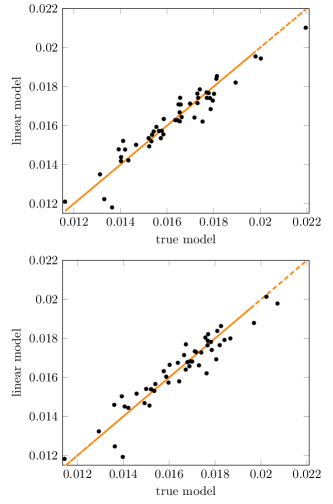
Figure 8: Fifty point comparison of the true model to the linear model for $S(t,{\mathchoice{\mbox{\boldmath$\displaystyle{\xi}$}}{\mbox{\boldmath$\textstyle{\xi}$}}{\mbox{\boldmath$\scriptstyle{\xi}$}}{\mbox{\boldmath$\scriptscriptstyle{\xi}$}}})$ at top: $t=400{,}234$ years, bottom: $t=500{,}106$ years.

In Figure 9, we report the screening indices that are above the importance threshold $tol=0.002$. The parameters with screening indices below $tol$ are considered unimportant. This reduces the input parameter dimension from ${{N}_{\text{p}}}=100$ to ${{n}_{\text{p}}}=10$ and the resulting reduced parameter is ${\mathchoice{\mbox{\boldmath$\displaystyle{\xi}$}}{\mbox{\boldmath$\textstyle{\xi}$}}{\mbox{\boldmath$\scriptstyle{\xi}$}}{\mbox{\boldmath$\scriptscriptstyle{\xi}$}}}^{r}=[\begin{matrix}\xi_{1}&\ldots&\xi_{10}\end{matrix}]^{T}$.

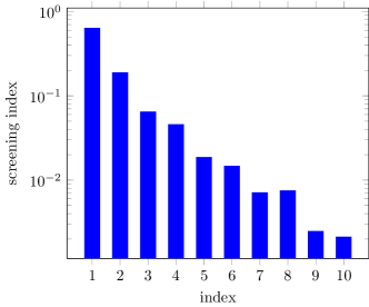
Figure 9: Screening indices $\mathfrak{s}_{j}$ for $S(t,{\mathchoice{\mbox{\boldmath$\displaystyle{\xi}$}}{\mbox{\boldmath$\textstyle{\xi}$}}{\mbox{\boldmath$\scriptstyle{\xi}$}}{\mbox{\boldmath$\scriptscriptstyle{\xi}$}}})$ calculated using Algorithm 2 with $500$ full QoI samples. Indices above $tol=0.002$ displayed only.

Spectral representation of the QoI. Next, we compute the KLE of $S(t,{\mathchoice{\mbox{\boldmath$\displaystyle{\xi}$}}{\mbox{\boldmath$\textstyle{\xi}$}}{\mbox{\boldmath$\scriptstyle{\xi}$}}{\mbox{\boldmath$\scriptscriptstyle{\xi}$}}})$ using Algorithm 1. This requires solving the eigenvalue problem (12), with $\mathcal{C}_{\text{qoi}}$ being the covariance operator of $S(t,{\mathchoice{\mbox{\boldmath$\displaystyle{\xi}$}}{\mbox{\boldmath$\textstyle{\xi}$}}{\mbox{\boldmath$\scriptstyle{\xi}$}}{\mbox{\boldmath$\scriptscriptstyle{\xi}$}}})$. We use a sample average approximation of $\mathcal{C}_{\text{qoi}}$ with sample size ${N}_{\text{s}}\in\{100,200,350,550\}$ exact QoI evaluations, as detailed in Algorithm 1. For this calculation we utilize the weights and nodes associated with the composite trapezoid rule. In Figure 10 (top), we show the computed (dominant) eigenvalues of $\mathcal{C}_{\text{qoi}}$. We note that the dominant eigenvalues are approximated well even with ${N}_{\text{s}}=100$. We use the computations corresponding ${N}_{\text{s}}=550$ in what follows. We note that the eigenvalues of the output covariance operator decay rapidly. We also report $r_{k}$ from equation (13), in Figure 10 (bottom). We note that $r_{k}$ exceeds $0.99$ for $k\geq 5$. This indicates that $S(t,{\mathchoice{\mbox{\boldmath$\displaystyle{\xi}$}}{\mbox{\boldmath$\textstyle{\xi}$}}{\mbox{\boldmath$\scriptstyle{\xi}$}}{\mbox{\boldmath$\scriptscriptstyle{\xi}$}}})$ is a low-rank process and a KL expansion with ${{N}_{\text{qoi}}}=5$ provides a suitable approximation of the QoI. Consequently, we consider the truncated KL expansion of $S(t,{\mathchoice{\mbox{\boldmath$\displaystyle{\xi}$}}{\mbox{\boldmath$\textstyle{\xi}$}}{\mbox{\boldmath$\scriptstyle{\xi}$}}{\mbox{\boldmath$\scriptscriptstyle{\xi}$}}})$

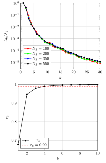
Figure 10: Top: comparison of ratio $\lambda_{k}/\lambda_{1}$, $k=1\ldots,30$ for $\lambda_{i}(\mathcal{C}_{\text{qoi}})$ corresponding to $S(t,{\mathchoice{\mbox{\boldmath$\displaystyle{\xi}$}}{\mbox{\boldmath$\textstyle{\xi}$}}{\mbox{\boldmath$\scriptstyle{\xi}$}}{\mbox{\boldmath$\scriptscriptstyle{\xi}$}}})$ computed with various sample sizes, bottom: $r_{k}$ as defined in (13), $k=1,\dots,10$, for $S(t,{\mathchoice{\mbox{\boldmath$\displaystyle{\xi}$}}{\mbox{\boldmath$\textstyle{\xi}$}}{\mbox{\boldmath$\scriptstyle{\xi}$}}{\mbox{\boldmath$\scriptscriptstyle{\xi}$}}})$. Dotted line corresponds to $0.99$.

$$S_{{{{{N}_{\text{qoi}}}}\!}}(t,{\mathchoice{\mbox{\boldmath$\displaystyle{\xi}$}}{\mbox{\boldmath$\textstyle{\xi}$}}{\mbox{\boldmath$\scriptstyle{\xi}$}}{\mbox{\boldmath$\scriptscriptstyle{\xi}$}}})=\bar{S}(t)+\sum_{i=1}^{{{N}_{\text{qoi}}}}\sqrt{\lambda_{i}(\mathcal{C}_{\text{qoi}})}S_{i}({\mathchoice{\mbox{\boldmath$\displaystyle{\xi}$}}{\mbox{\boldmath$\textstyle{\xi}$}}{\mbox{\boldmath$\scriptstyle{\xi}$}}{\mbox{\boldmath$\scriptscriptstyle{\xi}$}}})\Phi_{i}(t),$$ (29)

where ${{N}_{\text{qoi}}}=5$. The next step is to compute PCEs for the KL modes $S_{i}({\mathchoice{\mbox{\boldmath$\displaystyle{\xi}$}}{\mbox{\boldmath$\textstyle{\xi}$}}{\mbox{\boldmath$\scriptstyle{\xi}$}}{\mbox{\boldmath$\scriptscriptstyle{\xi}$}}})$, $i=1,\ldots,{{N}_{\text{qoi}}}$.

PCE surrogates of the KL modes. Next, we construct a bispectral surrogate for $S(t,{\mathchoice{\mbox{\boldmath$\displaystyle{\xi}$}}{\mbox{\boldmath$\textstyle{\xi}$}}{\mbox{\boldmath$\scriptstyle{\xi}$}}{\mbox{\boldmath$\scriptscriptstyle{\xi}$}}})$ which we denote $S_{{{{{N}_{\text{qoi}}}}\!}}^{\text{PC}}$. Recall that the components of ${\mathchoice{\mbox{\boldmath$\displaystyle{\xi}$}}{\mbox{\boldmath$\textstyle{\xi}$}}{\mbox{\boldmath$\scriptstyle{\xi}$}}{\mbox{\boldmath$\scriptscriptstyle{\xi}$}}}^{r}$ are sampled from a Gaussian distribution. Hence, we utilize the ${{n}_{\text{p}}}$-variate Hermite polynomials as the orthogonal basis for the PC expansions, with ${{n}_{\text{p}}}=10$. We use the sparse-regression approach (see Section 4.2) for computing PCEs of the output KL modes (see Section 5.2). To determine suitable values for the maximum polynomial degree ${N}_{\text{ord}}$ and the sparsity parameter $\tau$, we use a 10-fold cross validation procedure, which we briefly explain next.

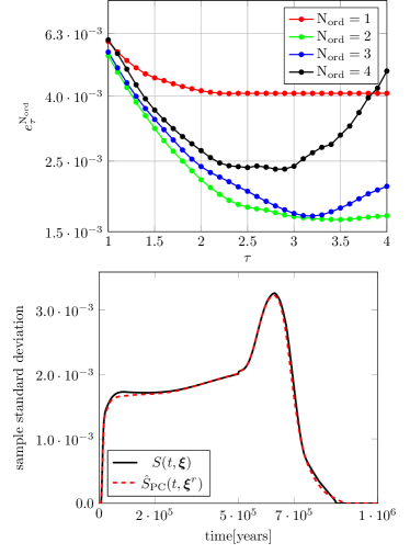
Figure 11: Top: cross-validation results for $\tau=\{1,1.1,\ldots,3.9,4\}$ and ${N}_{\text{ord}}=\{1,2,3,4\}$ for gas saturation, bottom: comparison of sample standard deviations of $S(t,{\mathchoice{\mbox{\boldmath$\displaystyle{\xi}$}}{\mbox{\boldmath$\textstyle{\xi}$}}{\mbox{\boldmath$\scriptstyle{\xi}$}}{\mbox{\boldmath$\scriptscriptstyle{\xi}$}}})$ and $S_{{{{{N}_{\text{qoi}}}}\!}}^{\text{PC}}(t,{\mathchoice{\mbox{\boldmath$\displaystyle{\xi}$}}{\mbox{\boldmath$\textstyle{\xi}$}}{\mbox{\boldmath$\scriptstyle{\xi}$}}{\mbox{\boldmath$\scriptscriptstyle{\xi}$}}}^{r})$ computed on $200$ sample points.

Note that for each evaluation of $S_{{{{{N}_{\text{qoi}}}}\!}}(t,{\mathchoice{\mbox{\boldmath$\displaystyle{\xi}$}}{\mbox{\boldmath$\textstyle{\xi}$}}{\mbox{\boldmath$\scriptstyle{\xi}$}}{\mbox{\boldmath$\scriptscriptstyle{\xi}$}}}_{j})$, $j=1,\ldots,{N}_{\text{s}}$, there is a corresponding KL mode evaluation $S_{i}({\mathchoice{\mbox{\boldmath$\displaystyle{\xi}$}}{\mbox{\boldmath$\textstyle{\xi}$}}{\mbox{\boldmath$\scriptstyle{\xi}$}}{\mbox{\boldmath$\scriptscriptstyle{\xi}$}}}_{j})$, for $i=1,\ldots,{{N}_{\text{qoi}}}$. We separate the parameter samples into $W=\{{\mathchoice{\mbox{\boldmath$\displaystyle{\xi}$}}{\mbox{\boldmath$\textstyle{\xi}$}}{\mbox{\boldmath$\scriptstyle{\xi}$}}{\mbox{\boldmath$\scriptscriptstyle{\xi}$}}}_{j}^{r}\}_{j=1}^{350}$ and $\hat{W}=\{{\mathchoice{\mbox{\boldmath$\displaystyle{\xi}$}}{\mbox{\boldmath$\textstyle{\xi}$}}{\mbox{\boldmath$\scriptstyle{\xi}$}}{\mbox{\boldmath$\scriptscriptstyle{\xi}$}}}_{j}^{r}\}_{j=351}^{550}$. Similarly, for each $i=1,\ldots{{N}_{\text{qoi}}}$, we have $F_{i}=\{S_{i}({\mathchoice{\mbox{\boldmath$\displaystyle{\xi}$}}{\mbox{\boldmath$\textstyle{\xi}$}}{\mbox{\boldmath$\scriptstyle{\xi}$}}{\mbox{\boldmath$\scriptscriptstyle{\xi}$}}}_{j})\}_{j=1}^{350}$ and $\hat{F}_{i}=\{S_{i}({\mathchoice{\mbox{\boldmath$\displaystyle{\xi}$}}{\mbox{\boldmath$\textstyle{\xi}$}}{\mbox{\boldmath$\scriptstyle{\xi}$}}{\mbox{\boldmath$\scriptscriptstyle{\xi}$}}}_{j})\}_{j=351}^{550}$.

We partition $W$ and $F_{i}$, $i=1,\ldots,{{N}_{\text{qoi}}}$ $10$ different ways, such that each data partition has a $35$ point validation set and a $315$ point training set. Let $W^{k}$ and $F_{i}^{k}$, denote the $k$th such data partition, $k=1,\ldots,10$. Next, for every combination of ${N}_{\text{ord}}\in\{1,\dots 4\}$, $\tau\in\{1,1.1,1.2,\ldots,3.9,4\}$, $k=1,\ldots,10$, and $i=1,\ldots,{{N}_{\text{qoi}}}$ we solve the optimization problem (15); in our computations, we use the solver SPGL1 PCE07 . For the components of that data vector of $\textstyle{d}$ in (15), we use the training set of $F_{i}^{k}$. Therefore, every combination of $k$, ${N}_{\text{ord}}$ and $\tau$ results in a surrogate model denoted as $g^{k}_{{N}_{\text{ord}},\tau}(s,{\mathchoice{\mbox{\boldmath$\displaystyle{\xi}$}}{\mbox{\boldmath$\textstyle{\xi}$}}{\mbox{\boldmath$\scriptstyle{\xi}$}}{\mbox{\boldmath$\scriptscriptstyle{\xi}$}}}^{r})$.

To assess the accuracy of each bispectral surrogate we compute the average relative error

$$e_{\text{rel}}(g^{k}_{{N}_{\text{ord}},\tau})\!=\!\displaystyle\left[\frac{\sum_{j=1}^{M}\int_{\mathscr{X}}\big{[}S(t,{\mathchoice{\mbox{\boldmath$\displaystyle{\xi}$}}{\mbox{\boldmath$\textstyle{\xi}$}}{\mbox{\boldmath$\scriptstyle{\xi}$}}{\mbox{\boldmath$\scriptscriptstyle{\xi}$}}}_{j})-g^{k}_{{N}_{\text{ord}},\tau}(s,{\mathchoice{\mbox{\boldmath$\displaystyle{\xi}$}}{\mbox{\boldmath$\textstyle{\xi}$}}{\mbox{\boldmath$\scriptstyle{\xi}$}}{\mbox{\boldmath$\scriptscriptstyle{\xi}$}}}_{j}^{r})\big{]}^{2}\,ds}{\sum_{j=1}^{M}\int_{\mathscr{X}}S(t,{\mathchoice{\mbox{\boldmath$\displaystyle{\xi}$}}{\mbox{\boldmath$\textstyle{\xi}$}}{\mbox{\boldmath$\scriptstyle{\xi}$}}{\mbox{\boldmath$\scriptscriptstyle{\xi}$}}}_{j})^{2}\,ds}\right]^{\scalebox{1.125}{$\frac{1}{2}$}},$$ (30)

where $\mathscr{X}=[0,T_{f}]$, $M=35$ and ${\mathchoice{\mbox{\boldmath$\displaystyle{\xi}$}}{\mbox{\boldmath$\textstyle{\xi}$}}{\mbox{\boldmath$\scriptstyle{\xi}$}}{\mbox{\boldmath$\scriptscriptstyle{\xi}$}}}_{j}$ is the input parameter in the full space corresponding to ${\mathchoice{\mbox{\boldmath$\displaystyle{\xi}$}}{\mbox{\boldmath$\textstyle{\xi}$}}{\mbox{\boldmath$\scriptstyle{\xi}$}}{\mbox{\boldmath$\scriptscriptstyle{\xi}$}}}_{j}^{r}$ in the validation set of $W^{k}$.

We repeat the process for each of the 10 partitions, and compute the average of $\text{e}_{\text{rel}}$ across all partitions

$$e_{\tau}^{{N}_{\text{ord}}}=\frac{1}{10}\sum_{k=1}^{10}e_{\text{rel}}(g^{k}_{{N}_{\text{ord}},\tau}).$$

The cross-validation errors corresponding to $S(t,{\mathchoice{\mbox{\boldmath$\displaystyle{\xi}$}}{\mbox{\boldmath$\textstyle{\xi}$}}{\mbox{\boldmath$\scriptstyle{\xi}$}}{\mbox{\boldmath$\scriptscriptstyle{\xi}$}}})$ are displayed in Figure 11. The smallest $e_{\tau}^{{N}_{\text{ord}}}$ corresponds with ${N}_{\text{ord}}=2$ and $\tau=3.5$.

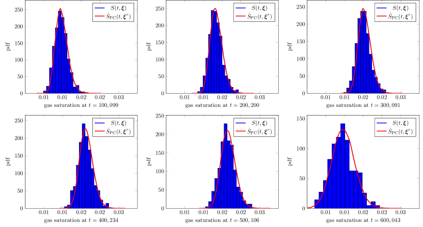
Figure 12: Comparison of normalized histograms for $S(t,{\mathchoice{\mbox{\boldmath$\displaystyle{\xi}$}}{\mbox{\boldmath$\textstyle{\xi}$}}{\mbox{\boldmath$\scriptstyle{\xi}$}}{\mbox{\boldmath$\scriptscriptstyle{\xi}$}}})$ and pdf estimates of the surrogate $S_{{{{{N}_{\text{qoi}}}}\!}}^{\text{PC}}(t,{\mathchoice{\mbox{\boldmath$\displaystyle{\xi}$}}{\mbox{\boldmath$\textstyle{\xi}$}}{\mbox{\boldmath$\scriptstyle{\xi}$}}{\mbox{\boldmath$\scriptscriptstyle{\xi}$}}}^{r})$ for a variety of times $t\in[0,T_{f}]$.

Computing the overall bispectral surrogate. Once we have determined appropriate values for ${N}_{\text{ord}}$ and $\tau$ we follow Algorithm 3 to construct a surrogate model from the truncated KLE expansion of the function-valued QoI. To determine PCE for each KL mode $S_{i}({\mathchoice{\mbox{\boldmath$\displaystyle{\xi}$}}{\mbox{\boldmath$\textstyle{\xi}$}}{\mbox{\boldmath$\scriptstyle{\xi}$}}{\mbox{\boldmath$\scriptscriptstyle{\xi}$}}})$, $i=1,\ldots,{{N}_{\text{qoi}}}$, we use the solver SPGL PCE07 to implement sparse linear regression over the entire 350 point data set $F_{i}$. We use the resulting expansions to form the overall bispectral surrogate:

$$S_{{{{{N}_{\text{qoi}}}}\!}}^{\text{PC}}=\bar{S}(t)+\sum_{i=1}^{{{N}_{\text{qoi}}}}\sqrt{\lambda(\mathcal{C}_{\text{qoi}})}S_{i}^{\text{PC}}({\mathchoice{\mbox{\boldmath$\displaystyle{\xi}$}}{\mbox{\boldmath$\textstyle{\xi}$}}{\mbox{\boldmath$\scriptstyle{\xi}$}}{\mbox{\boldmath$\scriptscriptstyle{\xi}$}}}^{r})\Phi_{i}(t).$$

Note that in numerical computations, $\bar{S}(t)$ is the sample mean $\bar{S}(t)=\frac{1}{{N}_{\text{s}}}\sum_{j=1}^{{N}_{\text{s}}}S(t,{\mathchoice{\mbox{\boldmath$\displaystyle{\xi}$}}{\mbox{\boldmath$\textstyle{\xi}$}}{\mbox{\boldmath$\scriptstyle{\xi}$}}{\mbox{\boldmath$\scriptscriptstyle{\xi}$}}}_{j})$.

Next, we assess the effectiveness of the bispectral surrogate to reflect the statistical properties of the true model. First, we compare the sample standard deviations of $S_{{{{{N}_{\text{qoi}}}}\!}}^{\text{PC}}(t,{\mathchoice{\mbox{\boldmath$\displaystyle{\xi}$}}{\mbox{\boldmath$\textstyle{\xi}$}}{\mbox{\boldmath$\scriptstyle{\xi}$}}{\mbox{\boldmath$\scriptscriptstyle{\xi}$}}}^{r})$ and $S(t,{\mathchoice{\mbox{\boldmath$\displaystyle{\xi}$}}{\mbox{\boldmath$\textstyle{\xi}$}}{\mbox{\boldmath$\scriptstyle{\xi}$}}{\mbox{\boldmath$\scriptscriptstyle{\xi}$}}})$ computed over the testing set $\hat{W}$. The results are shown in Figure 11 (bottom). Note, the surrogate model does an excellent job capturing the behavior of $S(t,{\mathchoice{\mbox{\boldmath$\displaystyle{\xi}$}}{\mbox{\boldmath$\textstyle{\xi}$}}{\mbox{\boldmath$\scriptstyle{\xi}$}}{\mbox{\boldmath$\scriptscriptstyle{\xi}$}}})$. Then, we compute the pdf of $S_{{{{{N}_{\text{qoi}}}}\!}}^{\text{PC}}(t,{\mathchoice{\mbox{\boldmath$\displaystyle{\xi}$}}{\mbox{\boldmath$\textstyle{\xi}$}}{\mbox{\boldmath$\scriptstyle{\xi}$}}{\mbox{\boldmath$\scriptscriptstyle{\xi}$}}}^{r})$ with $100{,}000$ surrogate evaluations and compare with the normalized histograms of the $550$ exact model evaluations. In Figure 12 clockwise from upper left we show the pdf estimates for a few representative simulation times. Note that pdf estimates closely match the distribution of the full model.

6.2 Gas flux at the outflow boundary

In this section, we study gas flux at the outflow boundary, denoted by $Q(t,{\mathchoice{\mbox{\boldmath$\displaystyle{\xi}$}}{\mbox{\boldmath$\textstyle{\xi}$}}{\mbox{\boldmath$\scriptstyle{\xi}$}}{\mbox{\boldmath$\scriptscriptstyle{\xi}$}}})$. A few realizations of $Q(t,{\mathchoice{\mbox{\boldmath$\displaystyle{\xi}$}}{\mbox{\boldmath$\textstyle{\xi}$}}{\mbox{\boldmath$\scriptstyle{\xi}$}}{\mbox{\boldmath$\scriptscriptstyle{\xi}$}}})$ are shown in Figure 5 (bottom). The global linear model is computed with $500$ model realizations. A representation of the linear model at time $t=500{,}106$ years is displayed in Figure 14 (top). Next, we compute the screening indices $\mathfrak{s}_{j}$. In Figure 14 (bottom) we display $\mathfrak{s}_{j}$, $j=1\ldots,10$ above $tol=0.02$ only. Therefore, dimension reduction results in the reduced input parameter ${\mathchoice{\mbox{\boldmath$\displaystyle{\xi}$}}{\mbox{\boldmath$\textstyle{\xi}$}}{\mbox{\boldmath$\scriptstyle{\xi}$}}{\mbox{\boldmath$\scriptscriptstyle{\xi}$}}}^{r}=[\begin{matrix}\xi_{1}&\ldots&\xi_{10}\end{matrix}]^{\mkern-1.5mu\mathsf{T}}$. Next, we compute the KLE and truncate at ${{N}_{\text{qoi}}}=7$ terms. Then, we construct the surrogate model using the data sets $W$ and $F_{i}$, where the $F_{i}$’s for this instance consist of the KL modes computed for $Q(t,{\mathchoice{\mbox{\boldmath$\displaystyle{\xi}$}}{\mbox{\boldmath$\textstyle{\xi}$}}{\mbox{\boldmath$\scriptstyle{\xi}$}}{\mbox{\boldmath$\scriptscriptstyle{\xi}$}}})$. We use the 10-fold cross-validation technique described in Section 6.1 to choose the sparse linear regression parameters ${N}_{\text{ord}}=2$ and $\tau=4$. Finally, we use these values to generate the bispectral surrogate $Q_{{{{{N}_{\text{qoi}}}}\!}}^{\text{PC}}(t,{\mathchoice{\mbox{\boldmath$\displaystyle{\xi}$}}{\mbox{\boldmath$\textstyle{\xi}$}}{\mbox{\boldmath$\scriptstyle{\xi}$}}{\mbox{\boldmath$\scriptscriptstyle{\xi}$}}}^{r})$.

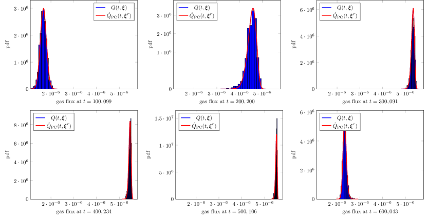
Figure 13: Comparison of normalized histograms for $Q(t,{\mathchoice{\mbox{\boldmath$\displaystyle{\xi}$}}{\mbox{\boldmath$\textstyle{\xi}$}}{\mbox{\boldmath$\scriptstyle{\xi}$}}{\mbox{\boldmath$\scriptscriptstyle{\xi}$}}})$ and pdf estimates of the surrogate $Q_{{{{{N}_{\text{qoi}}}}\!}}^{\text{PC}}(t,{\mathchoice{\mbox{\boldmath$\displaystyle{\xi}$}}{\mbox{\boldmath$\textstyle{\xi}$}}{\mbox{\boldmath$\scriptstyle{\xi}$}}{\mbox{\boldmath$\scriptscriptstyle{\xi}$}}}^{r})$ for a variety of times $t\in[0,T_{f}]$.

As before, to assess the effectiveness of the surrogate to capture the statistical properties of the true model we compare the sample standard deviation of the full model $Q(t,{\mathchoice{\mbox{\boldmath$\displaystyle{\xi}$}}{\mbox{\boldmath$\textstyle{\xi}$}}{\mbox{\boldmath$\scriptstyle{\xi}$}}{\mbox{\boldmath$\scriptscriptstyle{\xi}$}}})$ and the surrogate $Q_{{{{{N}_{\text{qoi}}}}\!}}^{\text{PC}}(t,{\mathchoice{\mbox{\boldmath$\displaystyle{\xi}$}}{\mbox{\boldmath$\textstyle{\xi}$}}{\mbox{\boldmath$\scriptstyle{\xi}$}}{\mbox{\boldmath$\scriptscriptstyle{\xi}$}}}^{r})$, computed on $200$ validation samples. Results are displayed in Figure 15 (bottom). Lastly, using $100{,}000$ samples of $Q_{{{{{N}_{\text{qoi}}}}\!}}^{\text{PC}}(t,{\mathchoice{\mbox{\boldmath$\displaystyle{\xi}$}}{\mbox{\boldmath$\textstyle{\xi}$}}{\mbox{\boldmath$\scriptstyle{\xi}$}}{\mbox{\boldmath$\scriptscriptstyle{\xi}$}}}^{r})$ we compute pdf estimates at equally spaced points in time and compare to normalized histograms created with $550$ full model evaluations; see Figure 13. The results in Figure 13 and Figure 15 demonstrate that the constructed surrogate for gas flux approximates the distribution of the full model reliably.

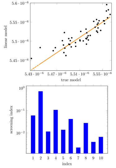
Figure 14: Top: comparison of the true model to the linear model for $Q(t,{\mathchoice{\mbox{\boldmath$\displaystyle{\xi}$}}{\mbox{\boldmath$\textstyle{\xi}$}}{\mbox{\boldmath$\scriptstyle{\xi}$}}{\mbox{\boldmath$\scriptscriptstyle{\xi}$}}})$ at $t=500{,}106$ years, bottom: screening indices for $Q(t,{\mathchoice{\mbox{\boldmath$\displaystyle{\xi}$}}{\mbox{\boldmath$\textstyle{\xi}$}}{\mbox{\boldmath$\scriptstyle{\xi}$}}{\mbox{\boldmath$\scriptscriptstyle{\xi}$}}})$.

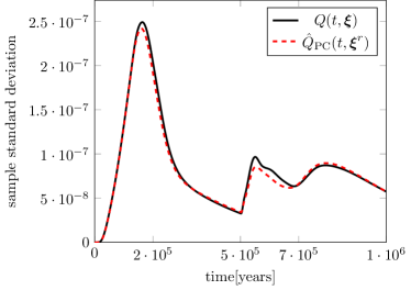
Figure 15: Comparison of sample standard deviations of $Q(t,{\mathchoice{\mbox{\boldmath$\displaystyle{\xi}$}}{\mbox{\boldmath$\textstyle{\xi}$}}{\mbox{\boldmath$\scriptstyle{\xi}$}}{\mbox{\boldmath$\scriptscriptstyle{\xi}$}}})$ and $Q_{{{{{N}_{\text{qoi}}}}\!}}^{\text{PC}}(t,{\mathchoice{\mbox{\boldmath$\displaystyle{\xi}$}}{\mbox{\boldmath$\textstyle{\xi}$}}{\mbox{\boldmath$\scriptstyle{\xi}$}}{\mbox{\boldmath$\scriptscriptstyle{\xi}$}}}^{r})$ computed with $200$ sample points.

6.3 Gas saturation across the domain

In this section, we focus on a spatially varying QoI. Let $S(x,{\mathchoice{\mbox{\boldmath$\displaystyle{\xi}$}}{\mbox{\boldmath$\textstyle{\xi}$}}{\mbox{\boldmath$\scriptstyle{\xi}$}}{\mbox{\boldmath$\scriptscriptstyle{\xi}$}}};t^{*})$ represent the QoI gas saturation across the spatial domain for a fixed time $t^{*}$. In particular, we include surrogate results at $t^{*}\in\{100{,}099\scalebox{1.5}{$,$}\,300{,}091\scalebox{1.5}{$,$}\,600{,}043\}$ years. We display several realizations for each QoI in Figure 17 (top). The surrogate models for spatial QoIs are computed via a similar procedure. Hence, for brevity, we include procedure details for $t^{*}=600{,}043$ years only. The relevant parameter values for the other QoIs are included in Table 2.

We consider the (spatial) global linear model for $S(x,{\mathchoice{\mbox{\boldmath$\displaystyle{\xi}$}}{\mbox{\boldmath$\textstyle{\xi}$}}{\mbox{\boldmath$\scriptstyle{\xi}$}}{\mbox{\boldmath$\scriptscriptstyle{\xi}$}}};t^{*})$. In Figure 16 (top) the linear model at $x=65.5$ meters is displayed. The global linear model was observed to perform similarly at other values of $x$. Next, we compute the screening indices $\mathfrak{s}_{j}$ and use the importance tolerance $tol=0.002$ for dimension reduction resulting in the reduced input parameter ${\mathchoice{\mbox{\boldmath$\displaystyle{\xi}$}}{\mbox{\boldmath$\textstyle{\xi}$}}{\mbox{\boldmath$\scriptstyle{\xi}$}}{\mbox{\boldmath$\scriptscriptstyle{\xi}$}}}^{r}=[\begin{matrix}\xi_{1}&\xi_{2}&\ldots&\xi_{8}\end{matrix}]^{\mkern-1.5mu\mathsf{T}}$. In Figure 16 (middle) we display the screening indices corresponding to these parameters.

Next, we compute the KLE of $S(x,{\mathchoice{\mbox{\boldmath$\displaystyle{\xi}$}}{\mbox{\boldmath$\textstyle{\xi}$}}{\mbox{\boldmath$\scriptstyle{\xi}$}}{\mbox{\boldmath$\scriptscriptstyle{\xi}$}}};t^{*})$ using Nyström’s method with $550$ model evaluations. In Figure 16 (bottom) we report the normalized eigenvalues of the output covariance operator $\mathcal{C}_{\text{qoi}}$ for $S(x,{\mathchoice{\mbox{\boldmath$\displaystyle{\xi}$}}{\mbox{\boldmath$\textstyle{\xi}$}}{\mbox{\boldmath$\scriptstyle{\xi}$}}{\mbox{\boldmath$\scriptscriptstyle{\xi}$}}};t^{*})$. This result is included to demonstrate that the gas saturation process is also low-rank in space. We truncate the KLE at ${{N}_{\text{qoi}}}=5$ terms.

As before, the PCE for the KL modes are computed with sparse linear regression using 350 full model realizations. Once again, the cross-validation procedure described in Section 6.1 is used to determine ${N}_{\text{ord}}=3$ and $\tau=2.8$. Lastly, the computed PCEs for each KL mode is used to construct the bispectral surrogate $S_{{{{{N}_{\text{qoi}}}}\!}}^{\text{PC}}(x,{\mathchoice{\mbox{\boldmath$\displaystyle{\xi}$}}{\mbox{\boldmath$\textstyle{\xi}$}}{\mbox{\boldmath$\scriptstyle{\xi}$}}{\mbox{\boldmath$\scriptscriptstyle{\xi}$}}}^{r})$.

surrogate	for fixed $t$ or $x$	${{N}_{\text{qoi}}}$	${N}_{\text{ord}}$	error
$S_{{{{{N}_{\text{qoi}}}}\!}}^{\text{PC}}(t,{\mathchoice{\mbox{\boldmath$\displaystyle{\xi}$}}{\mbox{\boldmath$\textstyle{\xi}$}}{\mbox{\boldmath$\scriptstyle{\xi}$}}{\mbox{\boldmath$\scriptscriptstyle{\xi}$}}})$	$x=0$ meters	$5$	2	$3.4813\cdot 10^{-2}$
$Q_{{{{{N}_{\text{qoi}}}}\!}}^{\text{PC}}(t,{\mathchoice{\mbox{\boldmath$\displaystyle{\xi}$}}{\mbox{\boldmath$\textstyle{\xi}$}}{\mbox{\boldmath$\scriptstyle{\xi}$}}{\mbox{\boldmath$\scriptscriptstyle{\xi}$}}})$	$x=200$ meters	$7$	2	$7.5019\cdot 10^{-3}$
$S_{{{{{N}_{\text{qoi}}}}\!}}^{\text{PC}}(x,{\mathchoice{\mbox{\boldmath$\displaystyle{\xi}$}}{\mbox{\boldmath$\textstyle{\xi}$}}{\mbox{\boldmath$\scriptstyle{\xi}$}}{\mbox{\boldmath$\scriptscriptstyle{\xi}$}}})$	$t^{*}=100{,}099$ years	$7$	2	$3.0397\cdot 10^{-2}$
$S_{{{{{N}_{\text{qoi}}}}\!}}^{\text{PC}}(x,{\mathchoice{\mbox{\boldmath$\displaystyle{\xi}$}}{\mbox{\boldmath$\textstyle{\xi}$}}{\mbox{\boldmath$\scriptstyle{\xi}$}}{\mbox{\boldmath$\scriptscriptstyle{\xi}$}}})$	$t^{*}=300{,}091$ years	$11$	2	$2.1690\cdot 10^{-2}$
$S_{{{{{N}_{\text{qoi}}}}\!}}^{\text{PC}}(x,{\mathchoice{\mbox{\boldmath$\displaystyle{\xi}$}}{\mbox{\boldmath$\textstyle{\xi}$}}{\mbox{\boldmath$\scriptstyle{\xi}$}}{\mbox{\boldmath$\scriptscriptstyle{\xi}$}}})$	$t^{*}=600{,}043$ years	$5$	3	$8.3110\cdot 10^{-2}$

Table 2: Surrogate parameter values and $\text{e}_{\text{rel}}$ errors for surrogate models.

To evaluate the effectiveness of the surrogate models for $t^{*}\in\{100{,}099\scalebox{1.5}{$,$}\,300{,}091\scalebox{1.5}{$,$}\,600{,}043\}$, we compare the sample standard deviation of $S(x,{\mathchoice{\mbox{\boldmath$\displaystyle{\xi}$}}{\mbox{\boldmath$\textstyle{\xi}$}}{\mbox{\boldmath$\scriptstyle{\xi}$}}{\mbox{\boldmath$\scriptscriptstyle{\xi}$}}};t^{*})$ and $S_{{{{{N}_{\text{qoi}}}}\!}}^{\text{PC}}(x,{\mathchoice{\mbox{\boldmath$\displaystyle{\xi}$}}{\mbox{\boldmath$\textstyle{\xi}$}}{\mbox{\boldmath$\scriptstyle{\xi}$}}{\mbox{\boldmath$\scriptscriptstyle{\xi}$}}}^{r})$ for 200 sample points. These results are displayed in Figure 17 (bottom). Observe, for $t^{*}=100{,}099$ and $t^{*}=300{,}091$ years the surrogate model replicates the sample standard deviation well. For $t^{*}=600{,}043$ years note that while we are underestimating the sample standard deviation, we are still capture the overall behavior of the full model.

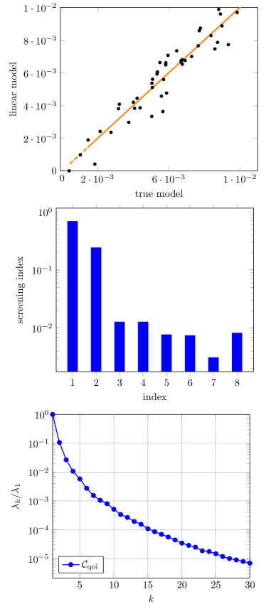
Figure 16: Results for $S(x,{\mathchoice{\mbox{\boldmath$\displaystyle{\xi}$}}{\mbox{\boldmath$\textstyle{\xi}$}}{\mbox{\boldmath$\scriptstyle{\xi}$}}{\mbox{\boldmath$\scriptscriptstyle{\xi}$}}};t^{*})$ with $t^{*}=600{,}043$ years. Top: comparison of the true model and the linear model for gas saturation across the domain, middle: screening indices for $S(x,{\mathchoice{\mbox{\boldmath$\displaystyle{\xi}$}}{\mbox{\boldmath$\textstyle{\xi}$}}{\mbox{\boldmath$\scriptstyle{\xi}$}}{\mbox{\boldmath$\scriptscriptstyle{\xi}$}}};t^{*})$, bottom: ratio $\lambda_{k}/\lambda_{1}$, $k=1,\ldots,30$ for $\lambda_{k}(\mathcal{C}_{\text{qoi}})$ corresponding to $S(x,{\mathchoice{\mbox{\boldmath$\displaystyle{\xi}$}}{\mbox{\boldmath$\textstyle{\xi}$}}{\mbox{\boldmath$\scriptstyle{\xi}$}}{\mbox{\boldmath$\scriptscriptstyle{\xi}$}}};t^{*})$.

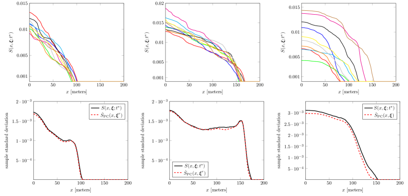
Figure 17: Top row, left to right: sample realizations of $S(x,{\mathchoice{\mbox{\boldmath$\displaystyle{\xi}$}}{\mbox{\boldmath$\textstyle{\xi}$}}{\mbox{\boldmath$\scriptstyle{\xi}$}}{\mbox{\boldmath$\scriptscriptstyle{\xi}$}}};t^{*})$ for times $100{,}099$, $300{,}091$, and $600{,}043$ years; bottom row, left to right: comparison of sample standard deviation of $S(x,{\mathchoice{\mbox{\boldmath$\displaystyle{\xi}$}}{\mbox{\boldmath$\textstyle{\xi}$}}{\mbox{\boldmath$\scriptstyle{\xi}$}}{\mbox{\boldmath$\scriptscriptstyle{\xi}$}}};t^{*})$ and $S_{{{{{N}_{\text{qoi}}}}\!}}^{\text{PC}}(x,{\mathchoice{\mbox{\boldmath$\displaystyle{\xi}$}}{\mbox{\boldmath$\textstyle{\xi}$}}{\mbox{\boldmath$\scriptstyle{\xi}$}}{\mbox{\boldmath$\scriptscriptstyle{\xi}$}}};t^{*})$ computed on $200$ sample points.

The capability of the computed bispectral surrogate to replicate true model behavior can also be tested by computing the average relative error defined in (30).Table 2 contains the values for $\text{e}_{\text{rel}}$ computed over the validation set $\hat{W}$ for each surrogate presented in this section, as well as those in Sections 6.1 and 6.2. Note that for the spatially varying QoIs, we let $\mathscr{X}=[0,200]$ and for temporally varying we let $\mathscr{X}=[0,T_{f}]$, in (30). Note, the error across all surrogates is less than 8%, and in four out the five surrogates is less than $4$%. The largest $\text{e}_{\text{rel}}$ corresponds to $S_{{{{{N}_{\text{qoi}}}}\!}}^{\text{PC}}(c,{\mathchoice{\mbox{\boldmath$\displaystyle{\xi}$}}{\mbox{\boldmath$\textstyle{\xi}$}}{\mbox{\boldmath$\scriptstyle{\xi}$}}{\mbox{\boldmath$\scriptscriptstyle{\xi}$}}})$ at $t=600{,}043$ years, in which case we are also underestimating the standard deviation.

6.4 Using the surrogate model

Here we illustrate the use of surrogates for temporally varying QoIs in performing statistical studies. In particular, we perform model prediction, variance-based global sensitivity analysis (GSA) by computing Sobol’ indices, and a study of output correlation structure. It is worth noting that Sobol’ indices can be computed analytically when using bispectral surrogates; see AlexanderianGremaudSmith20 . However, to keep the discussion general and since the cost of evaluating the bispectral surrogate is negligible, here we rely on sampling the bispectral surrogate for performing GSA. Specifically, we also perform GSA on QoIs that are derived from the bispectral surrogates such as maximum gas saturation and maximum gas flux at the outflow boundary.

Model prediction. We consider using $S_{{{{{N}_{\text{qoi}}}}\!}}^{\text{PC}}(t,{\mathchoice{\mbox{\boldmath$\displaystyle{\xi}$}}{\mbox{\boldmath$\textstyle{\xi}$}}{\mbox{\boldmath$\scriptstyle{\xi}$}}{\mbox{\boldmath$\scriptscriptstyle{\xi}$}}}^{r})$ and
$Q_{{{{{N}_{\text{qoi}}}}\!}}^{\text{PC}}(t,{\mathchoice{\mbox{\boldmath$\displaystyle{\xi}$}}{\mbox{\boldmath$\textstyle{\xi}$}}{\mbox{\boldmath$\scriptstyle{\xi}$}}{\mbox{\boldmath$\scriptscriptstyle{\xi}$}}}^{r})$ for making predictions. Recall, these bispectral surrogates correspond to gas saturation at the inflow boundary and gas flux at the outflow boundary. We study three observables of interest: maximum gas saturation, denoted $S_{\max}$, maximum gas flux, denoted $Q_{\max}$, and the first time for which gas saturation rises above 20% of $S_{\max}$. We compute $100{,}000$ realizations of each surrogate, extract the pertinent observables, and use the samples to compute pdf estimates. In Figure 18, we compare the pdf estimates against the normalized histograms computed using exact model evaluations. These results indicate the utility of the surrogates for estimating the statistical properties of model observables.

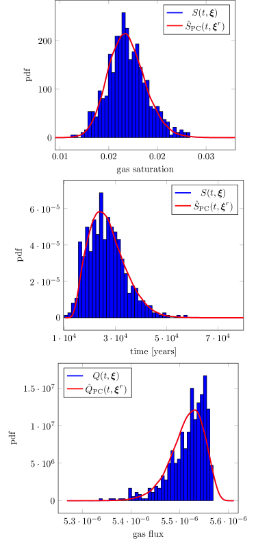
Figure 18: Comparison of normalized histograms and pdf estimates for top: max saturation value of $S_{\max}$, middle: first time $S_{{{{{N}_{\text{qoi}}}}\!}}^{\text{PC}}(t,\xi^{r})$ is above $20$% $S_{\max}$, bottom: max flux value $Q_{\max}$.

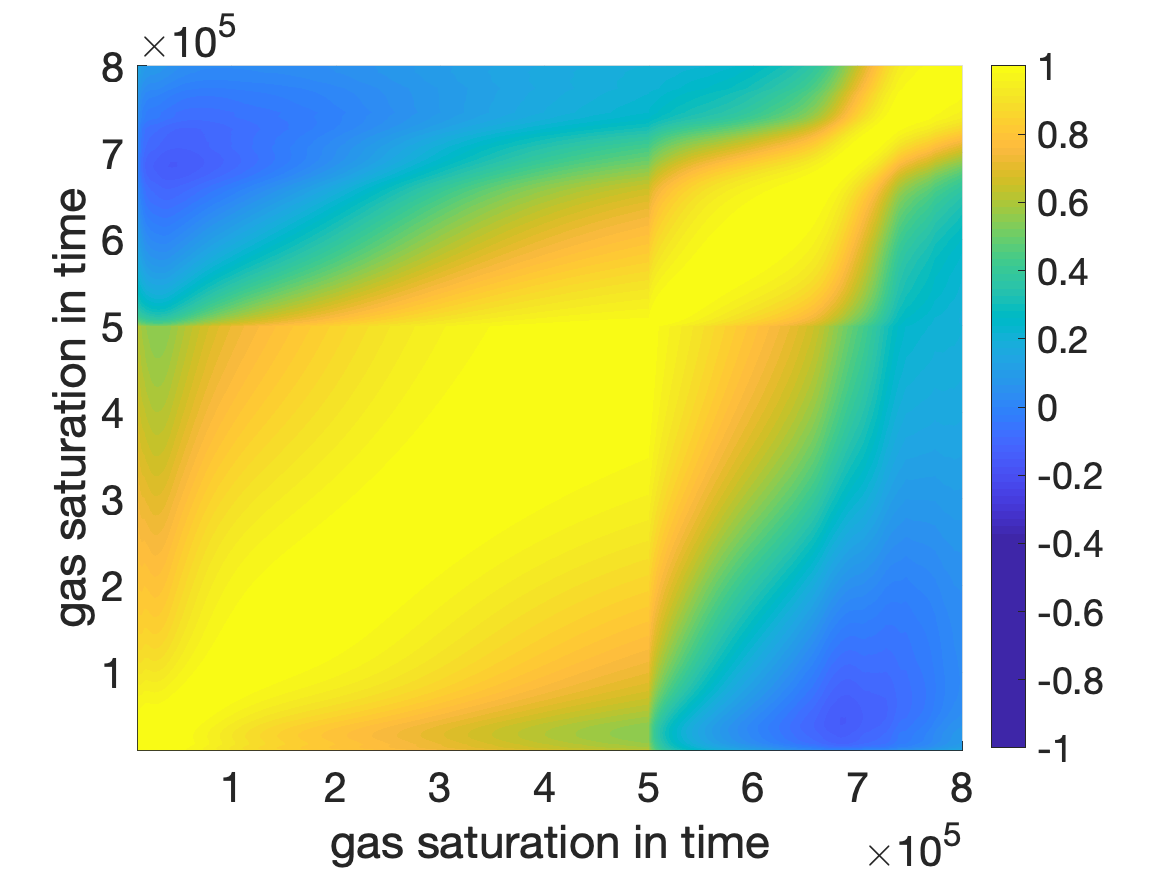
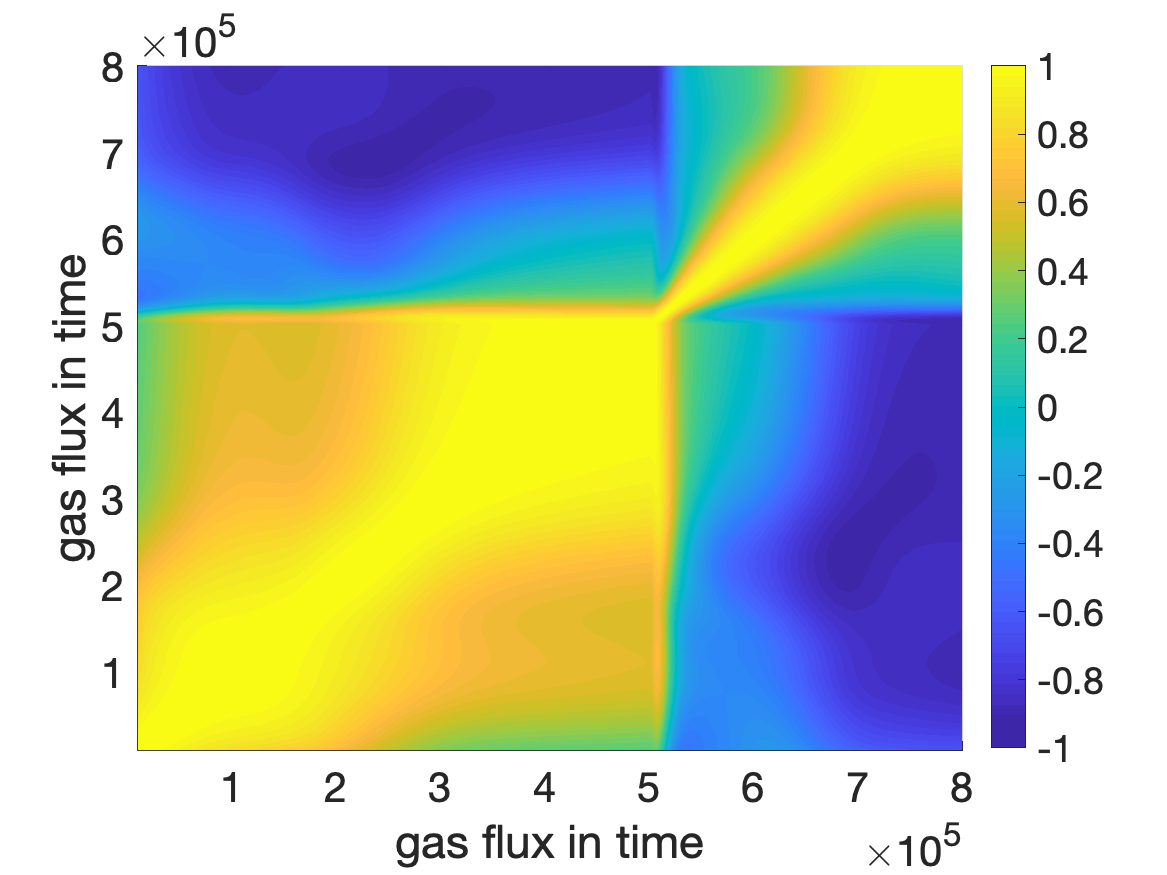
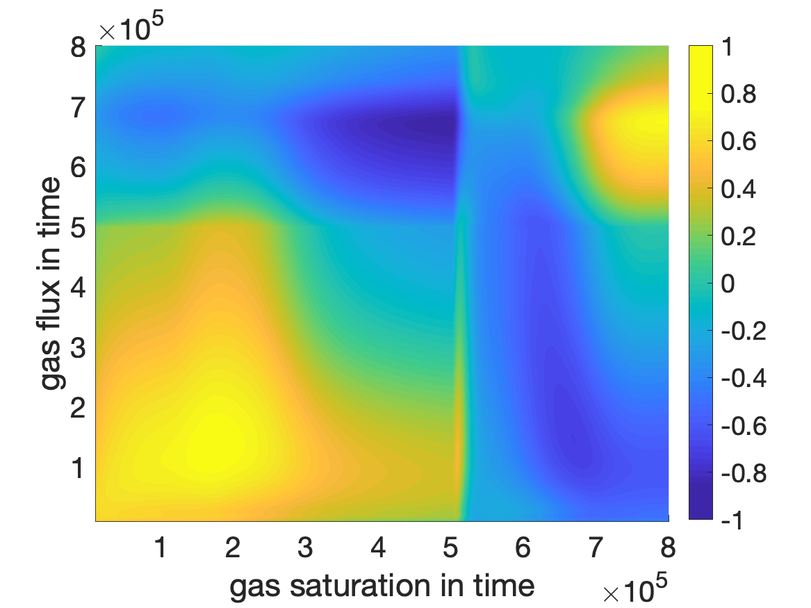
Figure 19: Top: correlation matrix for $S_{{{{{N}_{\text{qoi}}}}\!}}^{\text{PC}}(t,{\mathchoice{\mbox{\boldmath$\displaystyle{\xi}$}}{\mbox{\boldmath$\textstyle{\xi}$}}{\mbox{\boldmath$\scriptstyle{\xi}$}}{\mbox{\boldmath$\scriptscriptstyle{\xi}$}}}^{r})$ computed using the analytic formula in (27), middle: correlation matrix for $Q_{{{{{N}_{\text{qoi}}}}\!}}^{\text{PC}}(t,{\mathchoice{\mbox{\boldmath$\displaystyle{\xi}$}}{\mbox{\boldmath$\textstyle{\xi}$}}{\mbox{\boldmath$\scriptstyle{\xi}$}}{\mbox{\boldmath$\scriptscriptstyle{\xi}$}}}^{r})$ computed using the analytic formula in (27) bottom: cross-correlation structure of $S_{{{{{N}_{\text{qoi}}}}\!}}^{\text{PC}}(t,{\mathchoice{\mbox{\boldmath$\displaystyle{\xi}$}}{\mbox{\boldmath$\textstyle{\xi}$}}{\mbox{\boldmath$\scriptstyle{\xi}$}}{\mbox{\boldmath$\scriptscriptstyle{\xi}$}}}^{r})$ and $Q_{{{{{N}_{\text{qoi}}}}\!}}^{\text{PC}}(t,{\mathchoice{\mbox{\boldmath$\displaystyle{\xi}$}}{\mbox{\boldmath$\textstyle{\xi}$}}{\mbox{\boldmath$\scriptstyle{\xi}$}}{\mbox{\boldmath$\scriptscriptstyle{\xi}$}}}^{r})$ computed using the analytic formula in (28).

Variance based sensitivity analysis via Sobol’ indices. total Sobol’ indices provide an informative global sensitivity analysis tool that apportions percentages of QoI variance due to input parameter variations. While total Sobol’ indices are traditionally applied to scalar QoIs Sobol01 ; Sobol90 , there exist extensions for variance based analysis to function-valued QoIs GamboaJanonKlein14 ; AlexanderianGremaudSmith20 , referred to as functional total Sobol’ indices.

In general, calculating Sobol’ indices for computationally intensive models is challenging. This involves an expensive sampling procedure that requires a large number of model evaluations. An efficient-to-evaluate surrogate model can be used to accelerate this process. We use the temporal surrogates to compute total Sobol’ indices for both function-valued and scalar QoIs. In particular, we compute the functional total Sobol’ indices for $S_{{{{{N}_{\text{qoi}}}}\!}}^{\text{PC}}(t,{\mathchoice{\mbox{\boldmath$\displaystyle{\xi}$}}{\mbox{\boldmath$\textstyle{\xi}$}}{\mbox{\boldmath$\scriptstyle{\xi}$}}{\mbox{\boldmath$\scriptscriptstyle{\xi}$}}}^{r})$ and $Q_{{{{{N}_{\text{qoi}}}}\!}}^{\text{PC}}(t,{\mathchoice{\mbox{\boldmath$\displaystyle{\xi}$}}{\mbox{\boldmath$\textstyle{\xi}$}}{\mbox{\boldmath$\scriptstyle{\xi}$}}{\mbox{\boldmath$\scriptscriptstyle{\xi}$}}}^{r})$, both of which are functions in $t$, and we compute the total Sobol’ indices for the scalar QoIs $S_{\max}$ and $Q_{\max}$. In each case, we compute the total Sobol’ indices via sampling, using a variety of samples sizes: ${N}_{\text{s}}=\{1{,}000\scalebox{1.5}{$,$}\,10{,}000\scalebox{1.5}{$,$}\,50{,}000\}$.

The results in the top row of Figure 20 show the functional Sobol’ indices for $S_{{{{{N}_{\text{qoi}}}}\!}}^{\text{PC}}(t,{\mathchoice{\mbox{\boldmath$\displaystyle{\xi}$}}{\mbox{\boldmath$\textstyle{\xi}$}}{\mbox{\boldmath$\scriptstyle{\xi}$}}{\mbox{\boldmath$\scriptscriptstyle{\xi}$}}}^{r})$ and $Q_{{{{{N}_{\text{qoi}}}}\!}}^{\text{PC}}(t,{\mathchoice{\mbox{\boldmath$\displaystyle{\xi}$}}{\mbox{\boldmath$\textstyle{\xi}$}}{\mbox{\boldmath$\scriptstyle{\xi}$}}{\mbox{\boldmath$\scriptscriptstyle{\xi}$}}}^{r})$. Note that the magnitudes in the top row of Figure 20 are similar to those in Figure 9 and Figure 14. This provides further support for the original input parameter importance ranking and subsequent dimension reduction. In the bottom row of Figure 20 we report the total Sobol’ indices for $S_{\max}$ and $Q_{\max}$. We also note that for the gas saturation QoIs (Figure 20(left: top and bottom), the importance ranking of the input parameters is similar. In contrast, there is more variability in ranking for gas flux QoIs (Figure 20 (right: top and bottom).

Finally, we mention that for many applications, the total Sobol’ indices can be used for further input parameter dimension reduction. For the present model however, we did not reduce the input parameter further because the surrogate model computed was already efficient and sufficiently accurate.

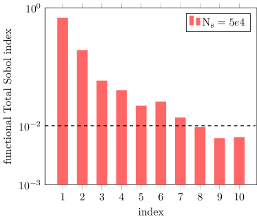
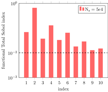
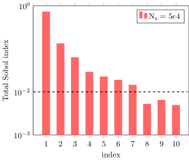
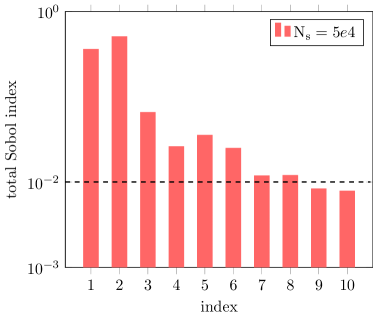
Figure 20: From top left counter clockwise: functional total Sobol’ indices for $S_{{{{{N}_{\text{qoi}}}}\!}}^{\text{PC}}(t,{\mathchoice{\mbox{\boldmath$\displaystyle{\xi}$}}{\mbox{\boldmath$\textstyle{\xi}$}}{\mbox{\boldmath$\scriptstyle{\xi}$}}{\mbox{\boldmath$\scriptscriptstyle{\xi}$}}}^{r})$, functional total Sobol’ indices for $Q_{{{{{N}_{\text{qoi}}}}\!}}^{\text{PC}}(t,{\mathchoice{\mbox{\boldmath$\displaystyle{\xi}$}}{\mbox{\boldmath$\textstyle{\xi}$}}{\mbox{\boldmath$\scriptstyle{\xi}$}}{\mbox{\boldmath$\scriptscriptstyle{\xi}$}}}^{r})$, total Sobol’ indices for $S_{\max}$, total Sobol’ indices for $Q_{\max}$.

Correlation structure Lastly, we illustrate the use of the bispectral surrogates for computing the correlation structure of the output, which is a useful tool for understanding overall model dynamics. Using equation (27) we compute the correlation function of $S_{{{{{N}_{\text{qoi}}}}\!}}^{\text{PC}}(t,{\mathchoice{\mbox{\boldmath$\displaystyle{\xi}$}}{\mbox{\boldmath$\textstyle{\xi}$}}{\mbox{\boldmath$\scriptstyle{\xi}$}}{\mbox{\boldmath$\scriptscriptstyle{\xi}$}}}^{r})$ and $Q_{{{{{N}_{\text{qoi}}}}\!}}^{\text{PC}}(t,{\mathchoice{\mbox{\boldmath$\displaystyle{\xi}$}}{\mbox{\boldmath$\textstyle{\xi}$}}{\mbox{\boldmath$\scriptstyle{\xi}$}}{\mbox{\boldmath$\scriptscriptstyle{\xi}$}}}^{r})$. The resulting heat maps are shown in Figure 19 top and middle, respectively. The results for $S_{{{{{N}_{\text{qoi}}}}\!}}^{\text{PC}}(t,{\mathchoice{\mbox{\boldmath$\displaystyle{\xi}$}}{\mbox{\boldmath$\textstyle{\xi}$}}{\mbox{\boldmath$\scriptstyle{\xi}$}}{\mbox{\boldmath$\scriptscriptstyle{\xi}$}}}^{r})$ suggest significant correlations across time. This behavior is also seen in the correlation function of $Q_{{{{{N}_{\text{qoi}}}}\!}}^{\text{PC}}(t,{\mathchoice{\mbox{\boldmath$\displaystyle{\xi}$}}{\mbox{\boldmath$\textstyle{\xi}$}}{\mbox{\boldmath$\scriptstyle{\xi}$}}{\mbox{\boldmath$\scriptscriptstyle{\xi}$}}}^{r})$, except the sudden shift in dynamics at the time $t=500{,}000$ years; recall, this the time gas injection stops. We also compute the cross-correlation between $S_{{{{{N}_{\text{qoi}}}}\!}}^{\text{PC}}(t,{\mathchoice{\mbox{\boldmath$\displaystyle{\xi}$}}{\mbox{\boldmath$\textstyle{\xi}$}}{\mbox{\boldmath$\scriptstyle{\xi}$}}{\mbox{\boldmath$\scriptscriptstyle{\xi}$}}}^{r})$ and $Q_{{{{{N}_{\text{qoi}}}}\!}}^{\text{PC}}(t,{\mathchoice{\mbox{\boldmath$\displaystyle{\xi}$}}{\mbox{\boldmath$\textstyle{\xi}$}}{\mbox{\boldmath$\scriptstyle{\xi}$}}{\mbox{\boldmath$\scriptscriptstyle{\xi}$}}}^{r})$ using the formula in (28); see Figure 19 (bottom). The heat map suggests there is large cross-correlation between the two QoI for both early and late times.

7 Conclusion

We have presented a structure exploiting non-intrusive framework for efficient dimension reduction and surrogate modeling for models with high-dimensional inputs and outputs. The proposed parameter screening metric utilizes approximate global sensitivity measures for function-valued outputs that rely on concepts from global sensitivity analysis and active subspace methods. An efficient bispectral surrogate model was constructed from a truncated KLE of the QoI by approximating the KL modes with PCEs. Note, these KL mode PCEs were constructed in the reduced parameter space.

We deployed our framework for fast uncertainty analysis in a multiphase multicomponent flow model. The efficiency and effectiveness of the surrogate model was demonstrated with a comprehensive set of numerical experiments, where we consider a number of function-valued (temporally or spatially distributed) QoIs. In particular, our results indicate that it is possible to use a modest amount of model realizations to reduce both the input and output dimensions and construct an efficient surrogate model. The proposed framework not only provides efficient surrogates, it also reveals and exploits the low-dimensional structures in model input and output spaces, which provides further insight into the behavior of the governing model.

In general, the screening approach takes the following form. We construct a cheap approximation $\tilde{f}$, compute the corresponding screening indices (22), and use them to reduce the input parameter space. Our approach relies on the screening metrics being sufficiently accurate surrogates and cheap to compute for the derivative-based global sensitivity measures for the function-valued QoIs under study. This in turn assumes the global linear model constructed within the parameter screening procedure leads to a sufficient approximation of the activity scores. It is observed that this global linear model can successfully capture one-dimensional active subspaces in a wide range of applications Constantine15 . The success of this strategy for obtaining approximate activity scores was also observed in the present work, in the context of a complex nonlinear flow model. However, for models that exhibit highly nonlinear parameter dependence a linear model might fail to provide accurate global sensitivity information. In GreyConstantine18 ; SeshadriSeshadriConstantineEtAl18 , global quadratic models were used effectively to accelerate active subspace discovery for scalar-valued QoIs. Exploring quadratic models within our framework provides an interesting direction for future work and would allow application of the proposed strategy to a broader class of problems.

Data availability

Data sharing is not applicable to this article as no datasets were generated or analysed during the current study. The results reported in this article are all based on numerical simulations. The details of the benchmark problem considered can be found in Bourgeat2012 .

8 Appendix

8.1 Proof of upper bound on total error in product space

Proof

Let $f(s,{\mathchoice{\mbox{\boldmath$\displaystyle{\xi}$}}{\mbox{\boldmath$\textstyle{\xi}$}}{\mbox{\boldmath$\scriptstyle{\xi}$}}{\mbox{\boldmath$\scriptscriptstyle{\xi}$}}})$ be in $L^{2}$ of the product space $\Theta\times\mathscr{X}$ and $\left\|\cdot\right\|$ be the $L^{2}$ error in the product space $\Theta\times\mathscr{X}$. The truncated KLE of $f$ is given by

$$f_{{{{{N}_{\text{qoi}}}}\!}}^{{\text{PC}}}(s,{\mathchoice{\mbox{\boldmath$\displaystyle{\xi}$}}{\mbox{\boldmath$\textstyle{\xi}$}}{\mbox{\boldmath$\scriptstyle{\xi}$}}{\mbox{\boldmath$\scriptscriptstyle{\xi}$}}})=\bar{f}(s)+\sum_{i=1}^{{{N}_{\text{qoi}}}}\sqrt{\lambda_{i}}f_{i}^{\text{PC}}({\mathchoice{\mbox{\boldmath$\displaystyle{\xi}$}}{\mbox{\boldmath$\textstyle{\xi}$}}{\mbox{\boldmath$\scriptstyle{\xi}$}}{\mbox{\boldmath$\scriptscriptstyle{\xi}$}}})\Phi_{i}(s).$$

The total error in the product space is given by

$$\left\|f-f_{{{{{N}_{\text{qoi}}}}\!}}^{{\text{PC}}}\right\|^{2}\leq 2\left\|f-f_{{{{{N}_{\text{qoi}}}}\!}}\right\|^{2}+2\left\|f_{{{{{N}_{\text{qoi}}}}\!}}-f_{{{{{N}_{\text{qoi}}}}\!}}^{{\text{PC}}}\right\|^{2}$$

We consider the first term

$$2\left\|f-f_{{{{{N}_{\text{qoi}}}}\!}}\right\|^{2}$$

$$= ~{}2\left\|\sum_{i=1}^{\infty}\sqrt{\lambda_{i}}f_{i}({\mathchoice{\mbox{\boldmath$\displaystyle{\xi}$}}{\mbox{\boldmath$\textstyle{\xi}$}}{\mbox{\boldmath$\scriptstyle{\xi}$}}{\mbox{\boldmath$\scriptscriptstyle{\xi}$}}})\Phi_{i}(s)-\sum_{i=1}^{{{N}_{\text{qoi}}}}\sqrt{\lambda_{i}}f_{i}({\mathchoice{\mbox{\boldmath$\displaystyle{\xi}$}}{\mbox{\boldmath$\textstyle{\xi}$}}{\mbox{\boldmath$\scriptstyle{\xi}$}}{\mbox{\boldmath$\scriptscriptstyle{\xi}$}}})\Phi_{i}(s)\right\|^{2}$$

$$= ~{}2\int_{\Theta}\int_{\mathscr{X}}\left(\sum_{i={{N}_{\text{qoi}}}+1}^{\infty}\sqrt{\lambda_{i}}f_{i}({\mathchoice{\mbox{\boldmath$\displaystyle{\xi}$}}{\mbox{\boldmath$\textstyle{\xi}$}}{\mbox{\boldmath$\scriptstyle{\xi}$}}{\mbox{\boldmath$\scriptscriptstyle{\xi}$}}})\Phi_{i}(s)\right)^{2}\,ds\,\!\upmu(d{\mathchoice{\mbox{\boldmath$\displaystyle{\xi}$}}{\mbox{\boldmath$\textstyle{\xi}$}}{\mbox{\boldmath$\scriptstyle{\xi}$}}{\mbox{\boldmath$\scriptscriptstyle{\xi}$}}})$$

$$= ~{}2\sum_{i,j={{N}_{\text{qoi}}}+1}^{\infty}\sqrt{\lambda_{i}}\sqrt{\lambda_{j}}\int_{\Theta}f_{i}({\mathchoice{\mbox{\boldmath$\displaystyle{\xi}$}}{\mbox{\boldmath$\textstyle{\xi}$}}{\mbox{\boldmath$\scriptstyle{\xi}$}}{\mbox{\boldmath$\scriptscriptstyle{\xi}$}}})f_{j}({\mathchoice{\mbox{\boldmath$\displaystyle{\xi}$}}{\mbox{\boldmath$\textstyle{\xi}$}}{\mbox{\boldmath$\scriptstyle{\xi}$}}{\mbox{\boldmath$\scriptscriptstyle{\xi}$}}})\int_{\mathscr{X}}\Phi_{i}(s)\Phi_{j}(s)\,ds\,\!\upmu(d{\mathchoice{\mbox{\boldmath$\displaystyle{\xi}$}}{\mbox{\boldmath$\textstyle{\xi}$}}{\mbox{\boldmath$\scriptstyle{\xi}$}}{\mbox{\boldmath$\scriptscriptstyle{\xi}$}}})$$

$$= ~{}2\sum_{i={{N}_{\text{qoi}}}+1}^{\infty}\lambda_{i}\int_{\Theta}f_{i}({\mathchoice{\mbox{\boldmath$\displaystyle{\xi}$}}{\mbox{\boldmath$\textstyle{\xi}$}}{\mbox{\boldmath$\scriptstyle{\xi}$}}{\mbox{\boldmath$\scriptscriptstyle{\xi}$}}})^{2}\,\!\upmu(d{\mathchoice{\mbox{\boldmath$\displaystyle{\xi}$}}{\mbox{\boldmath$\textstyle{\xi}$}}{\mbox{\boldmath$\scriptstyle{\xi}$}}{\mbox{\boldmath$\scriptscriptstyle{\xi}$}}})=~{}2\sum_{i={{N}_{\text{qoi}}}+1}^{\infty}\lambda_{i}.$$

Changing the order of infinite sums and integral is a consequence of the Dominated Convergence Theorem and reordering of integrals is a justified by Fubini’s Theorem. The orthogonality of the eigenfunctions in $L^{2}(\mathscr{X})$ justifies the simplification in the second to last line, and the last step is a consequence of the KL modes properties.

Next, we consider the second error term. Let

$$f_{i}^{\text{PC}}=\sum_{k=0}^{{N}_{\text{PC}}}\hat{c}_{i,k}\Psi_{k}({\mathchoice{\mbox{\boldmath$\displaystyle{\xi}$}}{\mbox{\boldmath$\textstyle{\xi}$}}{\mbox{\boldmath$\scriptstyle{\xi}$}}{\mbox{\boldmath$\scriptscriptstyle{\xi}$}}}),$$

where $\hat{c}_{i,k}$ represents the numerical approximation of the exact PCE coefficients $c_{i,k}$ and recall, $f_{i}=\sum_{k=0}^{\infty}c_{i,k}\Psi_{k}({\mathchoice{\mbox{\boldmath$\displaystyle{\xi}$}}{\mbox{\boldmath$\textstyle{\xi}$}}{\mbox{\boldmath$\scriptstyle{\xi}$}}{\mbox{\boldmath$\scriptscriptstyle{\xi}$}}})$ we have

$$~{}2\left\|f_{{{{{N}_{\text{qoi}}}}\!}}-f_{{{{{N}_{\text{qoi}}}}\!}}^{{\text{PC}}}\right\|^{2}=2\left\|\sum_{i=1}^{{{N}_{\text{qoi}}}}\sqrt{\lambda_{i}}f_{i}({\mathchoice{\mbox{\boldmath$\displaystyle{\xi}$}}{\mbox{\boldmath$\textstyle{\xi}$}}{\mbox{\boldmath$\scriptstyle{\xi}$}}{\mbox{\boldmath$\scriptscriptstyle{\xi}$}}})\Phi_{i}(s)-\sum_{i=1}^{{{N}_{\text{qoi}}}}\sqrt{\lambda_{i}}f_{i}^{\text{PC}}({\mathchoice{\mbox{\boldmath$\displaystyle{\xi}$}}{\mbox{\boldmath$\textstyle{\xi}$}}{\mbox{\boldmath$\scriptstyle{\xi}$}}{\mbox{\boldmath$\scriptscriptstyle{\xi}$}}})\Phi(s)\right\|^{2}$$

$$= ~{}2\int_{\Theta}\int_{\mathscr{X}}\left(\sum_{i=1}^{{{N}_{\text{qoi}}}}\sqrt{\lambda_{i}}\Phi_{i}(s)\left[f_{i}({\mathchoice{\mbox{\boldmath$\displaystyle{\xi}$}}{\mbox{\boldmath$\textstyle{\xi}$}}{\mbox{\boldmath$\scriptstyle{\xi}$}}{\mbox{\boldmath$\scriptscriptstyle{\xi}$}}})-f_{i}^{\text{PC}}({\mathchoice{\mbox{\boldmath$\displaystyle{\xi}$}}{\mbox{\boldmath$\textstyle{\xi}$}}{\mbox{\boldmath$\scriptstyle{\xi}$}}{\mbox{\boldmath$\scriptscriptstyle{\xi}$}}})\right]\right)^{2}\,ds\,\!\upmu(d{\mathchoice{\mbox{\boldmath$\displaystyle{\xi}$}}{\mbox{\boldmath$\textstyle{\xi}$}}{\mbox{\boldmath$\scriptstyle{\xi}$}}{\mbox{\boldmath$\scriptscriptstyle{\xi}$}}})$$

$$= ~{}2\sum_{i,j=1}^{{{N}_{\text{qoi}}}}\sqrt{\lambda_{i}}\sqrt{\lambda_{j}}\int_{\Theta}(f_{i}-f_{i}^{\text{PC}})(f_{j}-f_{j}^{\text{PC}})\int_{\mathscr{X}}\Phi_{i}(s)\Phi_{j}(s)\,ds\,\!\upmu(d{\mathchoice{\mbox{\boldmath$\displaystyle{\xi}$}}{\mbox{\boldmath$\textstyle{\xi}$}}{\mbox{\boldmath$\scriptstyle{\xi}$}}{\mbox{\boldmath$\scriptscriptstyle{\xi}$}}})$$

$$= ~{}2\sum_{i=1}^{{{N}_{\text{qoi}}}}\lambda_{i}\int_{\Theta}(f_{i}({\mathchoice{\mbox{\boldmath$\displaystyle{\xi}$}}{\mbox{\boldmath$\textstyle{\xi}$}}{\mbox{\boldmath$\scriptstyle{\xi}$}}{\mbox{\boldmath$\scriptscriptstyle{\xi}$}}})-f_{i}^{\text{PC}}({\mathchoice{\mbox{\boldmath$\displaystyle{\xi}$}}{\mbox{\boldmath$\textstyle{\xi}$}}{\mbox{\boldmath$\scriptstyle{\xi}$}}{\mbox{\boldmath$\scriptscriptstyle{\xi}$}}}))^{2}\,\!\upmu(d{\mathchoice{\mbox{\boldmath$\displaystyle{\xi}$}}{\mbox{\boldmath$\textstyle{\xi}$}}{\mbox{\boldmath$\scriptstyle{\xi}$}}{\mbox{\boldmath$\scriptscriptstyle{\xi}$}}})$$

$$= ~{}2\sum_{i=1}^{{{N}_{\text{qoi}}}}\lambda_{i}\int_{\Theta}\left(\sum_{k=0}^{\infty}c_{i,k}\Psi_{k}({\mathchoice{\mbox{\boldmath$\displaystyle{\xi}$}}{\mbox{\boldmath$\textstyle{\xi}$}}{\mbox{\boldmath$\scriptstyle{\xi}$}}{\mbox{\boldmath$\scriptscriptstyle{\xi}$}}})-\sum_{k=0}^{{N}_{\text{PC}}}\hat{c}_{i,k}\Psi_{k}({\mathchoice{\mbox{\boldmath$\displaystyle{\xi}$}}{\mbox{\boldmath$\textstyle{\xi}$}}{\mbox{\boldmath$\scriptstyle{\xi}$}}{\mbox{\boldmath$\scriptscriptstyle{\xi}$}}})\right)^{2}\,\,\!\upmu(d{\mathchoice{\mbox{\boldmath$\displaystyle{\xi}$}}{\mbox{\boldmath$\textstyle{\xi}$}}{\mbox{\boldmath$\scriptstyle{\xi}$}}{\mbox{\boldmath$\scriptscriptstyle{\xi}$}}})$$

$$= ~{}2\sum_{i=1}^{{{N}_{\text{qoi}}}}\lambda_{i}\int_{\Theta}\left(\sum_{k=0}^{{N}_{\text{PC}}}(c_{i,k}-\hat{c}_{i,k})\Psi_{k}({\mathchoice{\mbox{\boldmath$\displaystyle{\xi}$}}{\mbox{\boldmath$\textstyle{\xi}$}}{\mbox{\boldmath$\scriptstyle{\xi}$}}{\mbox{\boldmath$\scriptscriptstyle{\xi}$}}})+\sum_{k=1+{N}_{\text{PC}}}^{\infty}c_{i,k}\Psi_{k}({\mathchoice{\mbox{\boldmath$\displaystyle{\xi}$}}{\mbox{\boldmath$\textstyle{\xi}$}}{\mbox{\boldmath$\scriptstyle{\xi}$}}{\mbox{\boldmath$\scriptscriptstyle{\xi}$}}})\right)^{2}\,\!\upmu(d{\mathchoice{\mbox{\boldmath$\displaystyle{\xi}$}}{\mbox{\boldmath$\textstyle{\xi}$}}{\mbox{\boldmath$\scriptstyle{\xi}$}}{\mbox{\boldmath$\scriptscriptstyle{\xi}$}}})$$

$$= ~{}2\sum_{i=1}^{{{N}_{\text{qoi}}}}\lambda_{i}\sum_{k=1}^{{N}_{\text{PC}}}(c_{i,k}-\hat{c}_{i,k})^{2}\left\|\Psi_{k}\right\|_{L^{2}(\Theta)}^{2}$$

$$\hskip 42.67912pt+~{}2\sum_{i=1}^{{{N}_{\text{qoi}}}}\lambda_{i}\sum_{j=1+{N}_{\text{PC}}}^{\infty}c_{i,j}^{2}\left\|\Psi_{j}\right\|_{L^{2}(\Theta)}^{2}.$$

The simplification in the third line a consequence of the orthogonality of the PCE basis functions.

Thus, we have a bound on the total error

$$\left\|f-f_{{{{{N}_{\text{qoi}}}}\!}}^{{\text{PC}}}\right\|^{2}\leq 2\left\|f-f_{{{{{N}_{\text{qoi}}}}\!}}\right\|^{2}+2\left\|f_{{{{{N}_{\text{qoi}}}}\!}}-f_{{{{{N}_{\text{qoi}}}}\!}}^{{\text{PC}}}\right\|^{2}$$

$$=~{}2\sum_{i={{N}_{\text{qoi}}}+1}^{\infty}\lambda_{i}+\sum_{i=1}^{{{N}_{\text{qoi}}}}\lambda_{i}\sum_{k=1}^{{N}_{\text{PC}}}(c_{i,k}-\hat{c}_{i,k})^{2}\left\|\Psi_{k}\right\|_{L^{2}(\Theta)}^{2}$$

$$+2\sum_{i=1}^{{{N}_{\text{qoi}}}}\lambda_{i}\sum_{j=1+{N}_{\text{PC}}}^{\infty}c_{i,j}^{2}\left\|\Psi_{j}\right\|_{L^{2}(\Theta)}^{2}.~{}\square$$

References

- [1] Alen Alexanderian, Pierre Gremaud, and Ralph Smith. Variance-based sensitivity analysis for time-dependent processes. Reliability Engineering & System Safety, 2020.
- [2] Alen Alexanderian, William Reese, Ralph C Smith, and Meilin Yu. Model input and output dimension reduction using karhunen–loève expansions with application to biotransport. ASCE-ASME J Risk and Uncert in Engrg Sys Part B Mech Engrg, 5(4), 2019.
- [3] Alen Alexanderian, Justin Winokur, Ihab Sraj, Ashwanth Srinivasan, Mohamed Iskandarani, William C Thacker, and Omar M Knio. Global sensitivity analysis in an ocean general circulation model: a sparse spectral projection approach. Computational Geosciences, 16(3):757–778, 2012.
- [4] O. Angelini, C. Chavant, E. Chénier, R. Eymard, and S. Granet. Finite volume approximation of a diffusion-dissolution model and application to nuclear waste storage. Math. Comput. Simul., 81(10):2001–2017, 2011.
- [5] M. Saad B. Mansour Dia, B. Saad. Modeling and simulation of partially miscible two-phase flow with kinetics mass transfer. Mathematics and Computers in Simulation, 2020.
- [6] Wolfgang Betz, Iason Papaioannou, and Daniel Straub. Numerical methods for the discretization of random fields by means of the karhunen–loève expansion. Computer Methods in Applied Mechanics and Engineering, 271:109–129, 2014.
- [7] Géraud Blatman and Bruno Sudret. Efficient computation of global sensitivity indices using sparse polynomial chaos expansions. Reliability Engineering & System Safety, 95(11):1216–1229, 2010.
- [8] A. Bourgeat, S. Granet, and F. Smaï. Compositional two-phase flow in saturated-unsaturated porous media: benchmarks for phase appearance/disappearance. Radon Series on Computational and Applied Mathematics: Simulation of Flow in Porous Media, 2012.
- [9] A. Bourgeat, M. Jurak, and F. Smaï. Two-phase, partially miscible flow and transport modeling in porous media; application to gaz migration in a nuclear waste repository. Computational Geosciences, 6:309–325, 2009.
- [10] Mike Christie, Vasily Demyanov, and Demet Erbas. Uncertainty quantification for porous media flows. Journal of Computational Physics, 217(1):143–158, 2006.
- [11] Helen L. Cleaves, Alen Alexanderian, Hayley Guy, Ralph C. Smith, and Meilin Yu. Derivative-based global sensitivity analysis for models with high-dimension al inputs and functional outputs. SIAM Journal on Scientific Computing, 41:A3524–A3551, 2019.
- [12] Paul Constantine. Active Subspaces: Emerging Ideas for Dimension Reduction in Parameter Studies. Society for Industrial and Applied Mathematics, 2015.
- [13] Paul Constantine and Paul Diaz. Global sensitivity metrics from active subspaces. Reliability Engineering and System Safety, 162:1–13, 2017.
- [14] Antonio Costa. Permeability-porosity relationship: A reexamination of the kozeny-carman equation based on a fractal pore-space geometry assumption. Geophysical research letters, 33(2), 2006.
- [15] Thierry Crestaux, Olivier Le Maıtre, and Jean-Marc Martinez. Polynomial chaos expansion for sensitivity analysis. Reliability Engineering & System Safety, 94(7):1161–1172, 2009.
- [16] Noura Fajraoui, Stefano Marelli, and Bruno Sudret. Sequential design of experiment for sparse polynomial chaos expansions. SIAM/ASA Journal on Uncertainty Quantification, 5(1):1061–1085, 2017.
- [17] Fabrice Gamboa, Alexandre Janon, Thierry Klein, and Agnès Lagnoux. Sensitivity analysis for multidimensional and functional outputs. Electron. J. Statist., 8(1):575–603, 2014.
- [18] Zachary J Grey and Paul G Constantine. Active subspaces of airfoil shape parameterizations. AIAA Journal, 56(5):2003–2017, 2018.
- [19] Hayley Guy, Alen Alexanderian, and Meilin Yu. A distributed active subspace method for scalable surrogate modeling of function valued outputs. arXiv preprint arXiv:1908.02694, 2019.
- [20] JL Hart, PA Gremaud, and T David. Global sensitivity analysis of high-dimensional neuroscience models: An example of neurovascular coupling. Bulletin of mathematical biology, 81(6):1805–1828, 2019.
- [21] Jon C Helton. Uncertainty and sensitivity analysis techniques for use in performance assessment for radioactive waste disposal. Reliability Engineering & System Safety, 42(2-3):327–367, 1993.
- [22] Rainer Kress. Linear Integral Equations. Springer-Verlag New York, third edition, 2014.
- [23] S Kucherenko, María Rodriguez-Fernandez, C Pantelides, and Nilay Shah. Monte carlo evaluation of derivative-based global sensitivity measures. Reliability Engineering & System Safety, 94(7):1135–1148, 2009.
- [24] Sergey Kucherenko and Bertrand Iooss. Derivative-based global sensitivity measures. In R. Ghanem, D. Higdon, and H. Owhadi, editors, Handbook of Uncertainty Quantification. Springer, 2017.
- [25] Olivier Le Maître and Omar Knio. Spectral Methods for Uncertainty Quantification: With Applications to Computational Fluid Dynamics. Springer, 01 2010.
- [26] Guotu Li, Mohamed Iskandarani, Matthieu Le Hénaff, Justin Winokur, Olivier P Le Maître, and Omar M Knio. Quantifying initial and wind forcing uncertainties in the gulf of mexico. Computational Geosciences, 20(5):1133–1153, 2016.
- [27] Knut-Andreas Lie. An introduction to reservoir simulation using MATLAB/GNU Octave: User guide for the MATLAB Reservoir Simulation Toolbox (MRST). Cambridge University Press, 2019.
- [28] Michel Loève. Probability theory. I. Springer-Verlag, New York-Heidelberg, fourth edition, 1977. Graduate Texts in Mathematics, Vol. 45.
- [29] Habib N Najm. Uncertainty quantification and polynomial chaos techniques in computational fluid dynamics. Annual review of fluid mechanics, 41:35–52, 2009.
- [30] Argha Namhata, Sergey Oladyshkin, Robert M Dilmore, Liwei Zhang, and David V Nakles. Probabilistic assessment of above zone pressure predictions at a geologic carbon storage site. Scientific reports, 6(1):1–12, 2016.
- [31] Rebecca Neumann, Peter Bastian, and Olaf Ippisch. Modeling and simulation of two-phase two-component flow with disappearing nonwetting phase. Computational Geosciences, 17(1):139–149, 2012.
- [32] Bilal M Saad, Alen Alexanderian, Serge Prudhomme, and Omar M Knio. Probabilistic modeling and global sensitivity analysis for co2 storage in geological formations: a spectral approach. Applied Mathematical Modelling, 53:584–601, 2018.
- [33] Pranay Seshadri, Shahrokh Shahpar, Paul Constantine, Geoffrey Parks, and Mike Adams. Turbomachinery active subspace performance maps. Journal of Turbomachinery, 140(4), 2018.
- [34] Gerardo Severino, Santolo Leveque, and Gerardo Toraldo. Uncertainty quantification of unsteady source flows in heterogeneous porous media. Journal of Fluid Mechanics, 870:5–26, 2019.
- [35] I.M. Sobol. Estimation of the sensitivity of nonlinear mathematical models. Matematicheskoe Modelirovanie, 2(1):112–118, 1990.
- [36] I.M Sobol. Global sensitivity indices for nonlinear mathematical models and their Monte Carlo estimates. Mathematics and Computers in Simulation, 55(1–3):271–280, 2001. The Second IMACS Seminar on Monte Carlo Methods.
- [37] I.M. Sobol’ and S. Kucherenko. Derivative based global sensitivity measures and their link with global sensitivity indices. Mathematics and Computers in Simulation, 79(10):3009–3017, 2009.
- [38] Bruno Sudret. Global sensitivity analysis using polynomial chaos expansions. Reliability engineering & system safety, 93(7):964–979, 2008.
- [39] E. van den Berg and M. P. Friedlander. ”spgl1”: A solver for large-scale sparse reconstruction, 2007.
- [40] S Xiao, S Oladyshkin, and W Nowak. Reliability sensitivity analysis with subset simulation: application to a carbon dioxide storage problem. In IOP Conference Series: Materials Science and Engineering, volume 615, page 012051. IOP Publishing, 2019.
- [41] Liang Yan, Ling Guo, and Dongbin Xiu. Stochastic collocation algorithms using l1-minimization. International Journal for Uncertainty Quantification, 2(3):279–293, 2012.
- [42] Olivier Zahm, Paul G Constantine, Clementine Prieur, and Youssef M Marzouk. Gradient-based dimension reduction of multivariate vector-valued functions. SIAM Journal on Scientific Computing, 42(1):A534–A558, 2020.