Modeling Cell Populations Measured By Flow Cytometry With Covariates Using Sparse Mixture of Regressions

Abstract

The ocean is filled with microscopic microalgae called phytoplankton, which together are responsible for as much photosynthesis as all plants on land combined. Our ability to predict their response to the warming ocean relies on understanding how the dynamics of phytoplankton populations is influenced by changes in environmental conditions. One powerful technique to study the dynamics of phytoplankton is flow cytometry, which measures the optical properties of thousands of individual cells per second. Today, oceanographers are able to collect flow cytometry data in real-time onboard a moving ship, providing them with fine-scale resolution of the distribution of phytoplankton across thousands of kilometers. One of the current challenges is to understand how these small and large scale variations relate to environmental conditions, such as nutrient availability, temperature, light and ocean currents. In this paper, we propose a novel sparse mixture of multivariate regressions model to estimate the time-varying phytoplankton subpopulations while simultaneously identifying the specific environmental covariates that are predictive of the observed changes to these subpopulations. We demonstrate the usefulness and interpretability of the approach using both synthetic data and real observations collected on an oceanographic cruise conducted in the north-east Pacific in the spring of 2017.

Keywords: Mixture of regressions, Expectation-maximization, Flow cytometry, Sparse regression, Ocean, Microbiome, Phytoplankton, Clustering, Gating, Alternating direction method of multipliers

1 Introduction

Marine phytoplankton are responsible for as much photosynthesis as all plants on land combined, making them a crucial part of the earth’s biogeochemical cycle and climate (Field et al., 1998). A better understanding of the ecology of marine phytoplankton species and their relationship with the ocean environment is therefore important both to basic biology and to shedding light on their role in carbon dioxide uptake. In order to study these single cell organisms in the ocean, flow cytometry has been instrumental for the past three decades (Sosik et al., 2010).

Flow cytometry measures light scatter and fluorescence emission of individual cells at rates of up to thousands of cells per second. Light scattering is proportional to cell size, and fluorescence is unique to the emission spectra of pigments; these parameters can be used to identify populations of phytoplankton with similar optical properties. Over the two decades, automated environmental flow cytometers such as CytoBuoy (Dubelaar et al., 1999), FlowCytoBot (Olson et al., 2003), and SeaFlow (Swalwell et al., 2011) have provided an unprecedented view of dynamics of phytoplankton across large temporal and spatial scales.

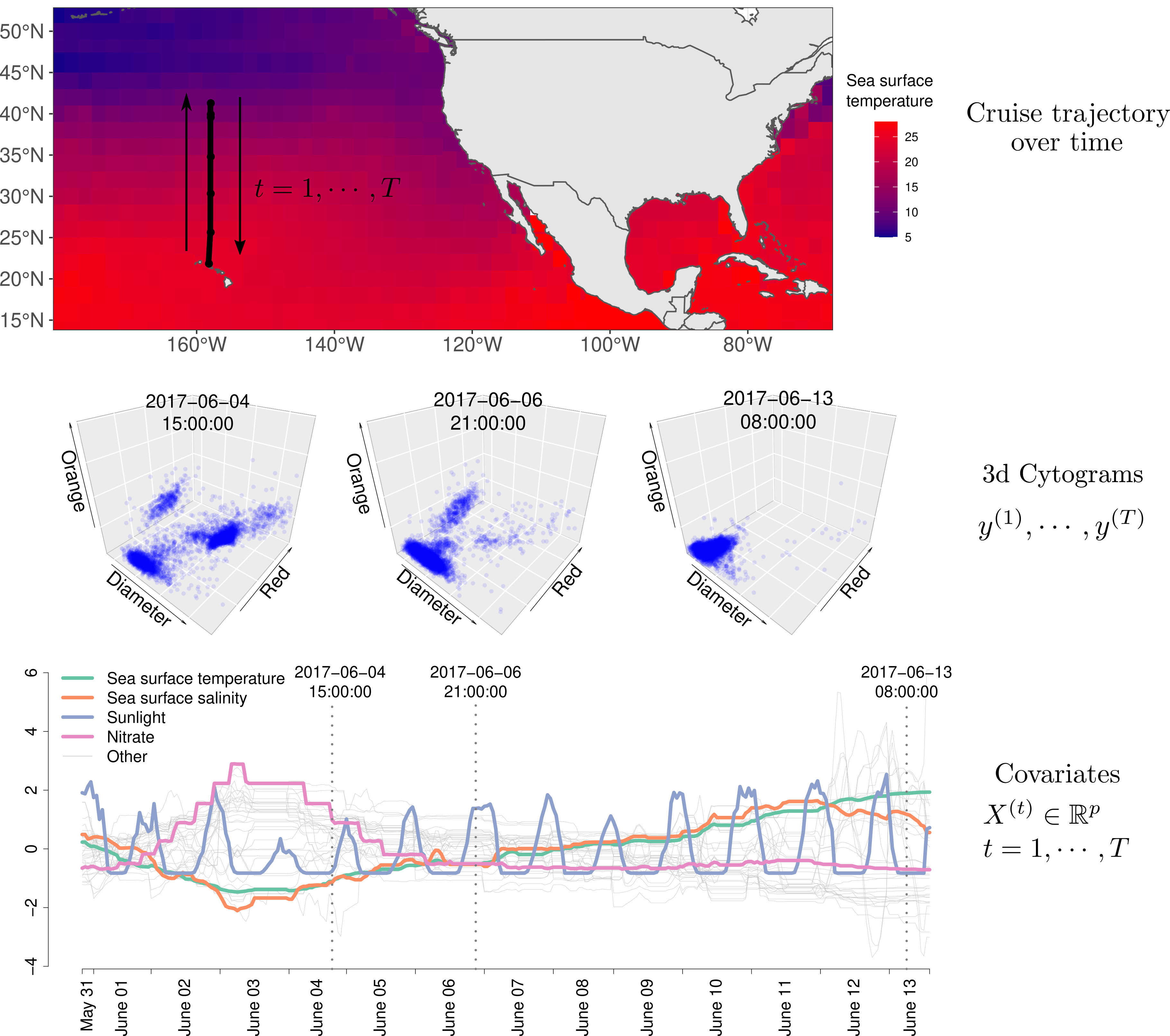
Figure 1: A schematic showing the data setup. (Top) This figure shows the trajectory of the Gradients 2 cruise, which moves North and then South along a trajectory starting at Hawaii. (Middle) The individual $3$-dimensional particles are measured rapidly and continuously. From this, we form $T$ cytograms $\mathbf{\color[rgb]{0,0,0}y}^{(t)},t=1,\cdots,T$ at an hourly time resolution. The three data dimensions have simplified labels Red, Orange, and Diameter; the first two represent fluorescence emission, and the last measures cell diameter. (Bottom panel) At each time $t=1,\cdots,T$, environmental covariates $\mathbf{\color[rgb]{0,0,0}X}^{(t)}\in\mathbb{R}^{p}$ are also available through remote sensing and on-board measurements. Only a few of the 30+ normalized covariates are highlighted here. Our proposed model identifies subpopulations by modeling them as Gaussian clusters whose means and probabilities are driven by environmental covariates.

Automated in-situ flow cytometry data can be represented as a scatterplot-valued time series, $\mathbf{\color[rgb]{0,0,0}y}^{(1)},\ldots,\mathbf{\color[rgb]{0,0,0}y}^{(T)}$, where an $n_{t}$ by $d$ matrix $\mathbf{\color[rgb]{0,0,0}y}^{(t)}$ whose rows are vectors $\{\mathbf{\color[rgb]{0,0,0}y}^{(t)}_{i}\in\mathbb{R}^{d}:i=1,\cdots,n_{t}\}$ is called a cytogram and can be thought of as a $d$-dimensional scatterplot representing $n_{t}$ particles observed during time interval $t$. The $d$ dimensions of the scatterplot represent $d$ optical properties that are useful in distinguishing different cell types from each other. Figure 1 shows an example of three cytograms collected by SeaFlow in June 2017 during a two-week cruise conducted in the Northeast Pacific. With SeaFlow, cytograms are of dimension $d=3$.

As apparent in the figure, the points within the cytograms display clear clustering structure. These different clusters correspond to cell populations of different types of phytoplankton. As the environmental conditions change, the populations change over time. In particular, in optical space, two noticeable phenomena over time are:

1. The number of cells in a given population can increase or decrease, with populations sometimes even appearing or disappearing entirely.

2. The centers of the cell populations are not fixed, but rather move over time.

Using expert knowledge and close manual inspection, oceanographers have been able to explain how some of these phenomena can be attributed to specific changes in environmental factors (e.g., oscillations in cell size due to sunlight and cell division) (Vaulot and Marie, 1999; Sosik et al., 2003; Ribalet et al., 2015).

Our goal is to develop a statistical approach for identifying how environmental factors can be predictive of changes to the cytograms. The promise of such a tool would be to discover new relationships between cell populations and environmental factors beyond those that may be known, or visible to the human eye.

Based on these observations and with this goal in mind, our statistical model for time-varying cytograms postulates a finite mixture model in which both the cluster probabilities and centers are allowed to vary over time. Changes to the cluster probabilities over time can capture the growing/shrinking and appearing/disappearing described above, while changes to the centers over time can capture the drifting/oscillating.

To be clear, our method does not explicitly incorporate the time (or space) aspect of the data. Instead, in our model, these cluster probabilities and centers are controlled by $p$ time-varying covariates $\mathbf{\color[rgb]{0,0,0}X}^{(t)}\in\mathbb{R}^{p}$. While our model can accommodate features that are purely functions of time (e.g., $\sin t$, $t^{2}$, spline basis functions, etc.), our focus here is on environmental covariates. Our analysis uses biological, physical, and chemical variables, shown in the bottom panel of Figure 1, that were retrieved from the Simons Collaborative Marine Atlas Project (CMAP) database (https://simonscmap.com), which is a public database compiling various oceanographic data over space and time.

One key strength of our method is the variable selection property, allowing the analyst to identify the subset of covariates that are the strongest predictor of each cluster’s mean and probability movement over time. For instance, in Figure 2, the estimated coefficients reveal that higher sea surface temperature and lower phosphate can predict a decrease in probability of cluster E located in the lower-left corner, and time-lagged sunlight and nitrate well predict the horizontal and vertical movement of cluster E’s center.

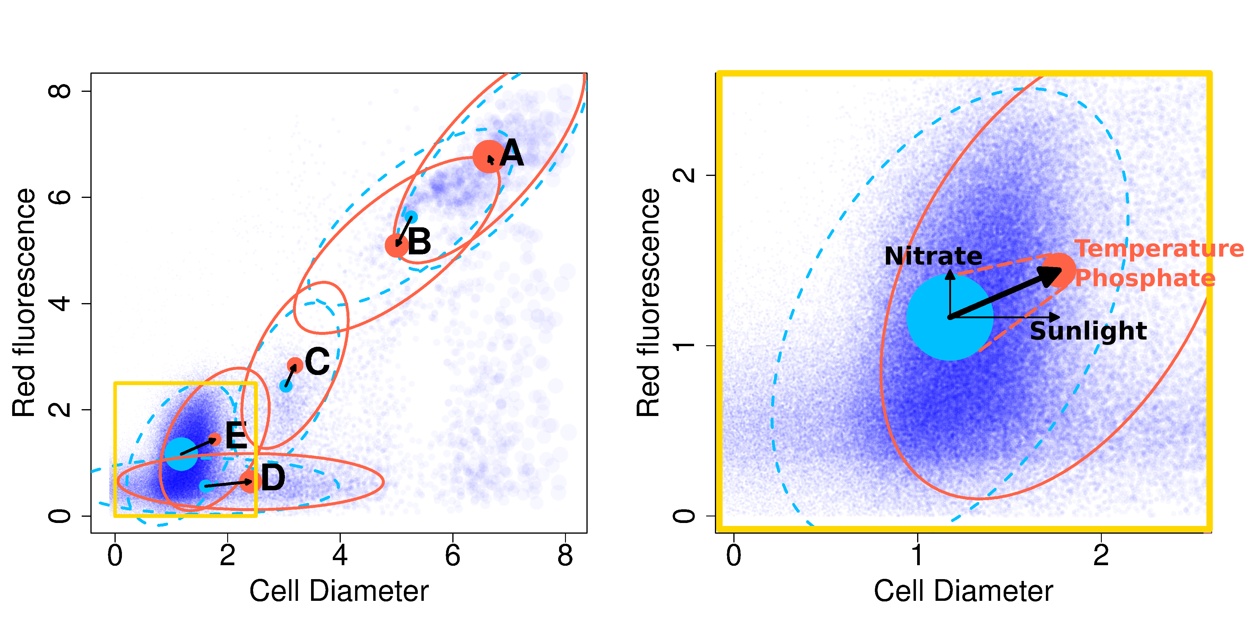
Figure 2: Our method produces estimates of cluster centers (shown as disks) and cluster probabilities (represented by the size of the disk) for every time point. The covariance of each mixture component (represented by an ellipse) is assumed to be constant over time. Blue and red show parameter estimates at two different time points. In the background, particles from only one time point are shown in (partially transparent) dark blue with the size of a point proportional to the particle’s biomass. The right figure takes a closer look at a subregion of the cytogram shown in the lower left corner of the left figure, focusing on cluster E which is a Prochlorococcus population. The change in the probability of cluster E is well predicted by sea surface temperature and phosphate, and the horizontal and vertical movement of cluster E’s center are each predicted by time-lagged sunlight and nitrate. Note, we are showing only five of the ten clusters used for estimation.

Our framework represents a substantial improvement in the detail and richness of how this data can be modeled and analyzed. Flow cytometry data are traditionally analyzed by a technique called gating, which counts the number of cells falling into certain fixed, expert-drawn polygonal regions of $\mathbb{R}^{d}$ corresponding to each cell population (Verschoor et al., 2015), reducing each scatterplot into several counts (giving the number of cells in each gated region) (Hyrkas et al., 2015). Subjectivity in manual gating has been shown to be an obstacle to reproducibility (Hahne et al., 2009). Furthermore, the presence of overlapping cell communities suggests that hard assignments to fixed disjoint regions may not be advisable. These and other shortcomings have led multiple authors to develop mixture model based approaches, as discussed in Aghaeepour et al. (2013). While such models are an improvement over traditional gating, they do not naturally extend to oceanography in which we have a time series of cytograms. Naively, one might think one could get away with fitting a separate mixture model to each individual cytogram. However, doing so leaves one with the problem of matching clusters from distinct clusterings, a task made particularly challenging since these clusters can move, change in size, and appear/disappear. Our approach fits a single mixture model jointly across the entire time series while integrating information from the covariates. By using all data sources in a single mixture model, our method is able to estimate the distinct components, even in cases where two populations’ centers may be nearby or a cluster may sometimes vanish.

In the statistics literature, the term finite mixture of regressions is used to refer to mixture models in which (univariate) means are modeled as functions of covariates (see, e.g., McLachlan and Peel 2006). Early works such as Wang et al. (1996) use information criteria and exhaustive search while more modern approaches have used penalized sparse models (Khalili and Chen, 2007; Städler et al., 2010). Our methodology differs from these methods in three respects: first, our means are multivariate ($d$-dimensional); second, the mixture weights are also modeled as functions of the covariates; third, the model coefficients are penalized. Of these, the first two aspects are shared by Grün and Leisch (2008), but without penalization. The idea of allowing the mixture weights to be functions of the features is more common in the machine learning literature, where such models are called mixtures of experts (Jordan and Jacobs, 1993).

To the best of our knowledge, this is the first attempt to extend mixture modeling of flow cytometry data by directly linking mixture model parameters with environmental covariates via sparse multivariate regression models. In Section 2, we describe our proposed model in detail. In section 3, we use our proposed model to draw rich new insights from a marine data source. We also conduct two realistic numerical simulations based on some pseudo-real ocean flow cytometry data. We provide an R package called flowmix that can be run both on a single machine, and also on remote high performance servers that use a parallel computing environment. While our focus is on time-varying flow cytometry in the ocean, our method can be applied more broadly to any collection of cytograms with associated covariates. For example, in biomedical applications each cytogram could correspond to a blood sample from a different person, and person-specific covariates could model the variability in cytograms.

2 Methodology

2.1 Likelihood function of cytogram

We model the $n_{t}$ particles $\{\mathbf{\color[rgb]{0,0,0}y}^{(t)}_{i}\}_{i=1}^{n_{t}}$ measured at time $t$ as i.i.d. draws from a probabilistic mixture of $K$ different $d$-variate Gaussian distributions, conditional on the covariate vector $\mathbf{\color[rgb]{0,0,0}X}^{(t)}\in\mathbb{R}^{p}$. The latent variable $Z_{i}^{(t)}$ determines the cluster membership,

$$P(Z_{i}^{(t)}=k|\mathbf{\color[rgb]{0,0,0}X}^{(t)})=\pi_{kt},\;k=1,\cdots,K,$$ (1)

and the data is drawn from the $k$’th Gaussian distribution,

$$(\mathbf{\color[rgb]{0,0,0}y}^{(t)}_{i}|\mathbf{\color[rgb]{0,0,0}X}^{(t)},Z_{i}^{(t)}=k)\sim\mathcal{N}_{d}\left(\boldsymbol{\color[rgb]{0,0,0}\mu}_{kt},\boldsymbol{\color[rgb]{0,0,0}\Sigma}_{k}\right),$$

where the cluster center $\boldsymbol{\color[rgb]{0,0,0}\mu}_{kt}\in\mathbb{R}^{d}$ and cluster probability $\pi_{kt}$ at time $t$ are modeled as functions of $\mathbf{\color[rgb]{0,0,0}X}^{(t)}$:

$$\boldsymbol{\color[rgb]{0,0,0}\mu}_{kt}(\beta) =\boldsymbol{\color[rgb]{0,0,0}\beta}_{0k}+\boldsymbol{\color[rgb]{0,0,0}\beta}_{k}^{T}\mathbf{\color[rgb]{0,0,0}X}^{(t)}$$

$$\pi_{kt}(\alpha) =\frac{\exp(\alpha_{0k}+{\mathbf{\color[rgb]{0,0,0}X}^{(t)}}^{T}\boldsymbol{\color[rgb]{0,0,0}\alpha}_{k})}{\sum_{l=1}^{K}\exp(\alpha_{0l}+{\mathbf{\color[rgb]{0,0,0}X}^{(t)}}^{T}\boldsymbol{\color[rgb]{0,0,0}\alpha}_{l})}$$

for regression coefficients $\boldsymbol{\color[rgb]{0,0,0}\beta}_{0k}\in\mathbb{R}^{d}$, $\boldsymbol{\color[rgb]{0,0,0}\beta}_{k}\in\mathbb{R}^{p\times d}$, $\boldsymbol{\color[rgb]{0,0,0}\alpha}_{k}\in\mathbb{R}^{p}$, and $\alpha_{0k}\in\mathbb{R}$; throughout, we use $\alpha$, $\beta$, and $\Sigma$ to denote the collection of coefficients $\{\alpha_{0k},\boldsymbol{\color[rgb]{0,0,0}\alpha}_{k}\}_{k=1}^{K}$, $\{\boldsymbol{\color[rgb]{0,0,0}\beta}_{0k},\boldsymbol{\color[rgb]{0,0,0}\beta}_{k}\}_{k=1}^{K}$, and $\{\boldsymbol{\color[rgb]{0,0,0}\Sigma}_{k}\}_{k=1}^{K}$ for brevity. Since all random variables are conditional on the covariates $\mathbf{\color[rgb]{0,0,0}X}^{(t)}$, we will omit it hereon for brevity. Denoting the density of the $k$’th Gaussian component of data at time $t$ as $\phi(\cdot;\boldsymbol{\color[rgb]{0,0,0}\mu}_{kt},\boldsymbol{\color[rgb]{0,0,0}\Sigma}^{(k)})$, the log-likelihood function is

$$\log\mathcal{L}(\alpha,\beta,\Sigma;\{\mathbf{\color[rgb]{0,0,0}y}_{i}^{(t)}\}_{i,t})=\sum_{t=1}^{T}\sum_{i=1}^{n_{t}}\log\left(\sum_{k=1}^{K}\pi_{kt}(\alpha)\cdot\phi\left(\mathbf{\color[rgb]{0,0,0}y}_{i}^{(t)};\boldsymbol{\color[rgb]{0,0,0}\mu}_{kt}(\beta),\boldsymbol{\color[rgb]{0,0,0}\Sigma}_{k}\right)\right).$$ (2)

By modeling the Gaussian means $\{\boldsymbol{\color[rgb]{0,0,0}\mu}_{kt}\}_{k,t}$ and mixture probabilities $\{\pi_{kt}\}_{k,t}$ as regression functions of $\mathbf{\color[rgb]{0,0,0}X}^{(t)}$ at each time point $t=1,\cdots,T$, our model directly allows environmental covariates to predict the two main kinds of cell population changes over time – movement in optical space, and change in relative population abundance. Furthermore, the signs and magnitudes of the entries of $\boldsymbol{\color[rgb]{0,0,0}\alpha}$ and $\boldsymbol{\color[rgb]{0,0,0}\beta}$ directly quantify the contribution of environment covariates to each population’s abundance and direction of movement in cytogram space.

2.2 Penalties and constraints

In practice, there are a large number of environmental covariates that may in principle be predictive of a cytogram. Also, the number of regression parameters is $(p+1)(d+1)K$, which can be large relative to the number of cytograms $T$. Furthermore, we would prefer models in which only a small number of parameters is nonzero. Therefore, we penalize the log-likelihood with lasso penalties (Tibshirani, 1996) on $\alpha$ and $\beta$.

In our application, each cell population has a limited range in optical properties, due to biological constraints. We incorporate this domain knowledge into the model by constraining the range of $\boldsymbol{\color[rgb]{0,0,0}\mu}_{k1},\cdots,\boldsymbol{\color[rgb]{0,0,0}\mu}_{kT}$ over time. Since $\boldsymbol{\color[rgb]{0,0,0}\beta}_{k}^{T}\mathbf{\color[rgb]{0,0,0}X}^{(t)}=\boldsymbol{\color[rgb]{0,0,0}\mu}_{kt}-\boldsymbol{\color[rgb]{0,0,0}\beta}_{0k}$, limiting the size of $\boldsymbol{\color[rgb]{0,0,0}\beta}_{k}^{T}\mathbf{\color[rgb]{0,0,0}X}^{(t)}$ is equivalent to limiting the deviation of the $k$’th cluster mean at all times $t=1,\cdots,T$ away from the overall center $\boldsymbol{\color[rgb]{0,0,0}\beta}_{0k}$. Motivated by this, we add a hard constraint so that $\|\boldsymbol{\color[rgb]{0,0,0}\beta}_{k}^{T}\mathbf{\color[rgb]{0,0,0}X}^{(t)}\|_{2}\leq r$ for some fixed radius value $r>0$.

The choice of $r$ should be specific to the data application. For 1-dimensional cytograms of cell diameter measurements used in the analysis in Section 4.0.1, the size of $r$ holds the intuitive meaning of not allowing the average optical properties of a particular cell population to deviate more than a multiplicative upper and lower bound over time compared to an overall average.

The constraint also plays an important role for model interpretability. We wish for the $k$’th mixture component to correspond to the same cell population over all time. When a cell population vanishes we would like $\pi_{kt}$ to go to zero rather than for $\boldsymbol{\color[rgb]{0,0,0}\mu}_{kt}$ to move to an entirely different place in cytogram space.

Our estimator is thus a solution to the following optimization problem: —l— α, β, Σ-1N logL(α, β, Σ; {y_i^(t)}_i,t ) + λ_α ∑_k=1^K∥ α_k ∥_1 + λ_β ∑_k=1^K∥β_k∥_1. ∥ β_k^T X^(t) ∥_2 ≤r    ∀t=1,⋯, T   ∀k = 1, ⋯, K. We divide the log-likelihood term by $N:=\sum_{t=1}^{T}n_{t}$ to make the scale consistent with that of a single particle.

2.3 Multiplicity generalization

Cytogram datasets can be extremely large, and cell populations can have highly imbalanced probabilities. To overcome the computational and methodological difficulties posed by these issues, we generalize the model to assign to particle $\mathbf{\color[rgb]{0,0,0}y}_{i}^{(t)}$ a multiplicity factor $C_{i}^{(t)}$ (which defaults to $1$).The log-likelihood in (2) becomes,

$$\ell_{(n_{1},\cdots,n_{T})}(\alpha,\beta,\Sigma;(\mathbf{\color[rgb]{0,0,0}y}^{(1)},\cdots,\mathbf{\color[rgb]{0,0,0}y}^{(T)}),(\mathbf{\color[rgb]{0,0,0}C}^{(1)},\cdots,\mathbf{\color[rgb]{0,0,0}C}^{(T)}))=\\ \sum_{t=1}^{T}\sum_{i=1}^{n_{t}}C_{i}^{(t)}\log\left(\sum_{k=1}^{K}\pi_{kt}(\alpha)\cdot\phi\left(\mathbf{\color[rgb]{0,0,0}y}_{i}^{(t)};\boldsymbol{\color[rgb]{0,0,0}\mu}_{kt}(\beta),\boldsymbol{\color[rgb]{0,0,0}\Sigma}_{k}\right)\right).$$ (3)

where $\mathbf{\color[rgb]{0,0,0}y}^{(t)}\in\mathbb{R}^{n_{t}\times d}$ and $\mathbf{\color[rgb]{0,0,0}C}^{(t)}\in\mathbb{R}^{n_{t}}$. Furthermore, the scaling by $N$ in the optimization objective (2.2) is generalized to $N:=\sum_{t=1}^{T}\sum_{i=1}^{n_{t}}C_{i}^{(t)}$, the overall sum of the multiplicities.

The multiplicity generalization is useful for an approximate data representation by placing particles in bins and dealing with bin counts. We discretize cytogram space along a lattice of $B=D^{d}$ $d$-dimensional cubes $\{E_{b}\}_{b=1}^{B}$ whose centers $\tilde{\mathbf{\color[rgb]{0,0,0}y}}_{b}\in\mathbb{R}^{d}$ can be arranged as the rows of a matrix $\tilde{\mathbf{\color[rgb]{0,0,0}y}}\in\mathbb{R}^{B\times d}$. This coarsened data representation involves counts $\{C_{b}^{(t)}\}_{b,t}$ of the number of particles in each fixed bin $E_{b}$:

$$C_{b}^{(t)}=\sum_{i=1}^{n_{t}}\mathds{1}\{i:\mathbf{\color[rgb]{0,0,0}y}_{i}^{(t)}\in E_{b}\},$$

whose collection is $\mathbf{\color[rgb]{0,0,0}C}^{(t)}\in\mathbb{R}^{B}$. Using $C_{b}^{(t)}$ and $\tilde{\mathbf{\color[rgb]{0,0,0}y}}_{b}^{(t)}:=\tilde{\mathbf{\color[rgb]{0,0,0}y}}_{b}$ to replace $C_{i}^{(t)}$ and $\mathbf{\color[rgb]{0,0,0}y}_{i}^{(t)}$ in (3), we obtain the log-likelihood of the binned data,

$$\ell_{(B,\cdots,B)}\left(\alpha,\beta,\Sigma;(\tilde{\mathbf{\color[rgb]{0,0,0}y}},\cdots,\tilde{\mathbf{\color[rgb]{0,0,0}y}}),(\mathbf{\color[rgb]{0,0,0}C}^{(1)},\cdots,\mathbf{\color[rgb]{0,0,0}C}^{(T)})\right)\\ =\sum_{t=1}^{T}\sum_{b=1}^{B}C_{b}^{(t)}\log\left(\sum_{k=1}^{K}\pi_{kt}(\alpha)\cdot\phi\left(\tilde{\mathbf{\color[rgb]{0,0,0}y}}_{b};\boldsymbol{\color[rgb]{0,0,0}\mu}_{kt}(\beta),\boldsymbol{\color[rgb]{0,0,0}\Sigma}_{k}\right)\right).$$ (4)

Whereas before each cytogram required its own set of $n_{t}$ particle locations, in the binned data representation, the same set of locations are shared across all $t$, which is indicated by the notation $(\tilde{y},\dots,\tilde{y})$.

This binned likelihood is identical to the original log-likelihood (2) after replacing each particle by its bin center. The computational savings are apparent from noticing that $\sum_{b=1}^{B}\mathds{1}\{C_{b}^{(t)}\neq 0\}\ll n_{t}$ since typically only a small subset of the bins $\{E_{b}\}$ contain any particles. Additionally, the number of Gaussian density calculations are reduced by a factor of $T$, since the particles $\tilde{\mathbf{\color[rgb]{0,0,0}y}}_{b}$ do not depend on $t$.

There is no finite value of $B$ for which the binned log-likelihood in (4) is equal to the log-likelihood calculated on the original data, due to the nonzero distance between bin centers $\tilde{\mathbf{\color[rgb]{0,0,0}y}}_{b}$ and data $\mathbf{\color[rgb]{0,0,0}y}_{i}^{(t)}$ even for very large $B$. However, the following proposition 1 establishes that parameter estimation from the binned data is asymptotically equivalent to parameter estimation from the original data, as the number of bins $B$ grows to $\infty$. The proof is provided in Supplement A. As for what occurs for finite values of $B$, a simulation study in Supplement F suggests that even using a relatively small number of bins can achieve similar predictive performance as using the original data.

Proposition 1.

Let

$$\tilde{\Theta}_{B}:=\mathop{\mathrm{argmin}}_{(\alpha,\beta,\Sigma)\in\Theta}\;\;-\frac{1}{N}\ell_{(B,\cdots,B)}\left(\alpha,\beta,\Sigma;(\tilde{\mathbf{\color[rgb]{0,0,0}y}},\cdots,\tilde{\mathbf{\color[rgb]{0,0,0}y}}),(\mathbf{\color[rgb]{0,0,0}C}^{(1)},\cdots,\mathbf{\color[rgb]{0,0,0}C}^{(T)})\right)+g(\alpha,\beta)$$ (5)

be the set of minimizers of the penalized negative log-likelihood of the binned data, and let

$$\hat{\Theta}:=\mathop{\mathrm{argmin}}_{(\alpha,\beta,\Sigma)\in\Theta}\;\;-\frac{1}{N}\log\mathcal{L}(\alpha,\beta,\Sigma;\{\mathbf{\color[rgb]{0,0,0}y}_{i}^{(t)}\}_{i,t})+g(\alpha,\beta),$$ (6)

be that of the original data. The term $g(\alpha,\beta)$ encapsulates the penalties on $\alpha$ and $\beta$ and the constraint on $\beta$ in (2.2). Assume the following:

1. The parameter space $\Theta$ of $(\alpha,\beta,\Sigma)$ is compact, and $\{\lambda_{\text{min}}(\boldsymbol{\color[rgb]{0,0,0}\Sigma}_{k})<c\}\cap\Theta=\emptyset$ for all $k=1,\cdots,K$, for some constant $c>0$.

2. The data belongs to a compact set $\mathcal{Y}$ with $\max_{\mathbf{\color[rgb]{0,0,0}y},\mathbf{\color[rgb]{0,0,0}y}^{\prime}\in\mathcal{Y}}\|\mathbf{\color[rgb]{0,0,0}y}-\mathbf{\color[rgb]{0,0,0}y}^{\prime}\|_{\infty}\leq R$ for some positive constant $R<\infty$.

3. The log likelihood $\log\mathcal{L}(\alpha,\beta,\Sigma;\{\mathbf{\color[rgb]{0,0,0}y}_{i}^{(t)}\}_{i,t})<\infty$ for all $(\alpha,\beta,\Sigma)\in\Theta$.

Then, given any sequence $\tilde{\theta}_{B}\in\tilde{\Theta}_{B}(B=1,2,\cdots)$ of minimizers of the penalized negative log-likelihood of the binned data, a sequence $s_{B}$ exists such that the subsequence $\tilde{\theta}_{s_{B}}$ converges to an element in $\hat{\Theta}$:

$$\lim_{B\to\infty}\tilde{\theta}_{s_{B}}\in\hat{\Theta}.$$ (7)

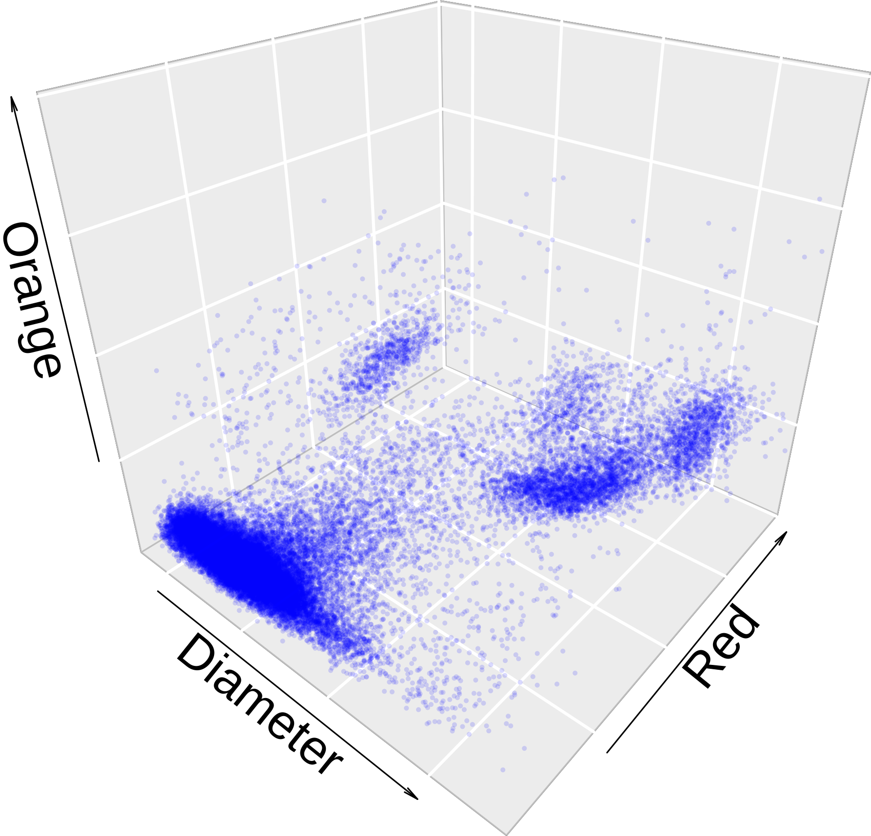
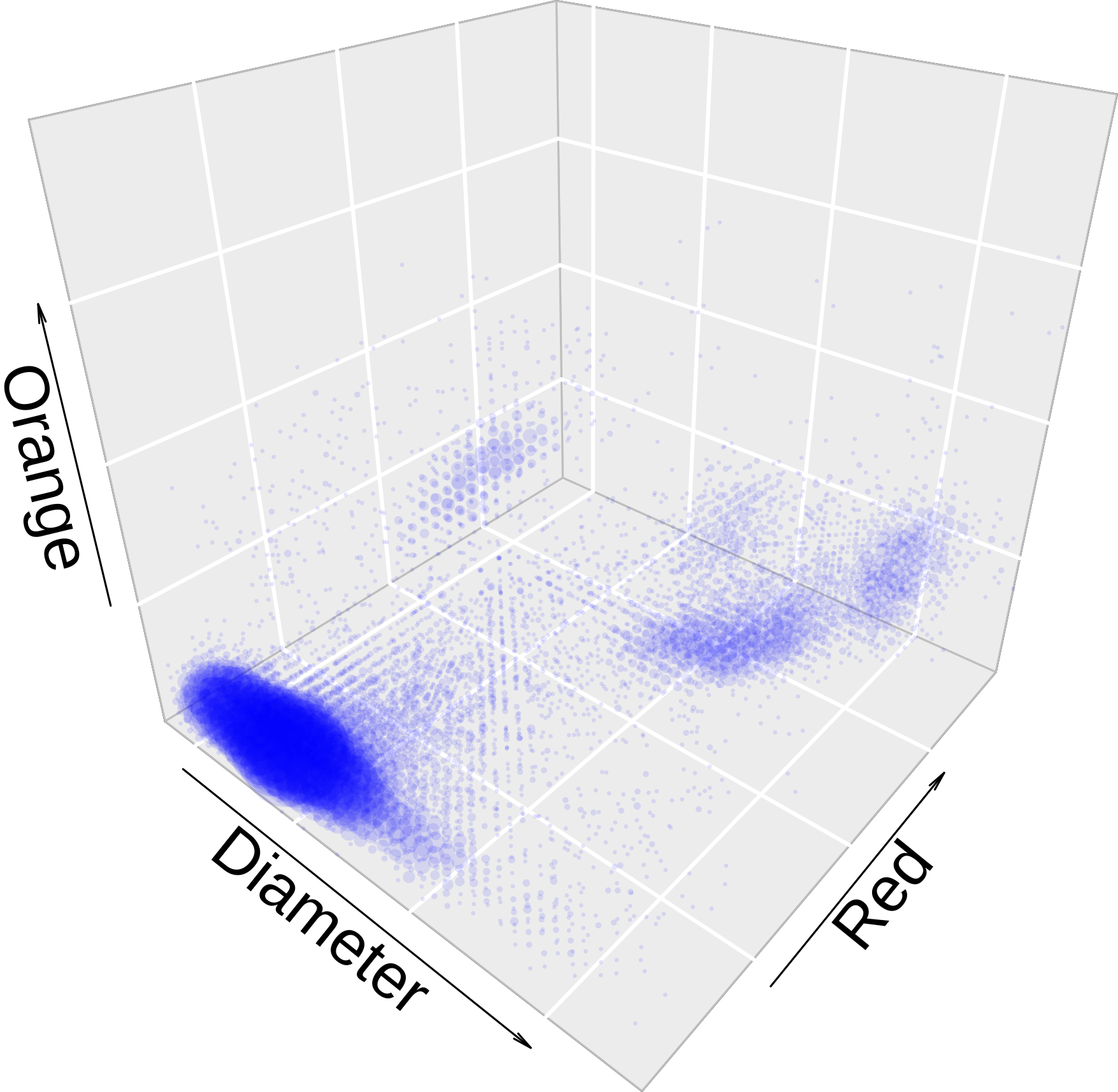
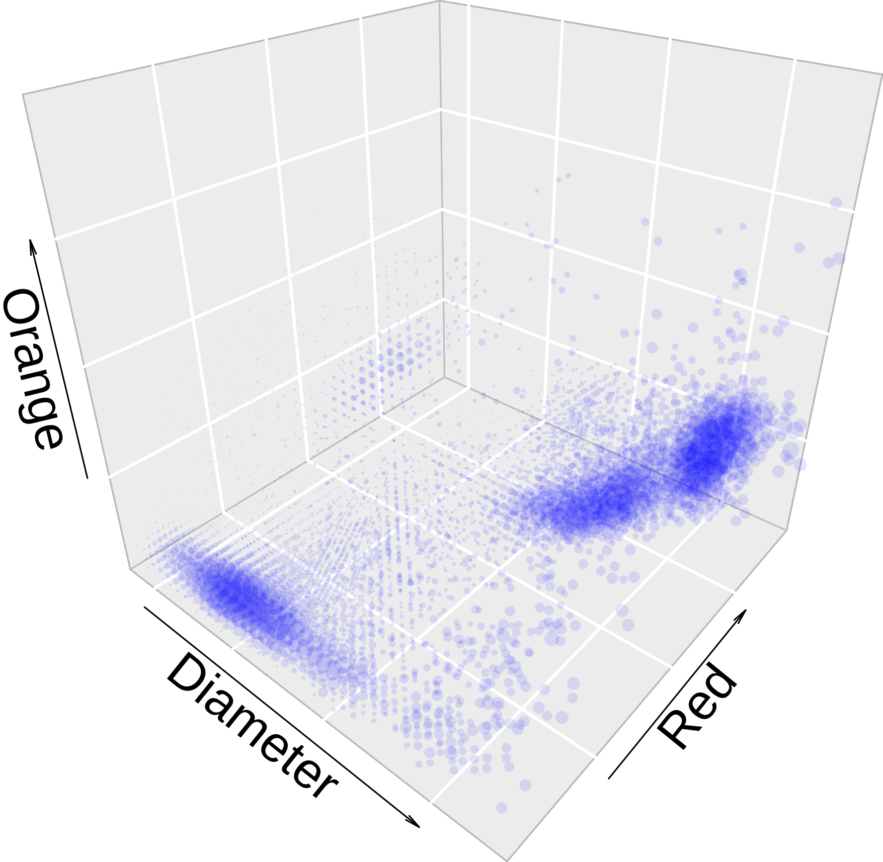
Figure 3: Original particles (left) and binned counts with $D=40$ (middle), and binned biomass (right). In the middle and right plots, the size of the points are proportional to the multiplicity. The left-hand-side original cytogram contain one hour’s worth of particles, for a total of $n_{t}=36,757$ points, occupying a total of $0.86$ Mb of memory. The binned cytogram in the middle occupies about $1/8$’th the memory. The right hand side shows binned biomass data, which has lesser imbalance in cluster distribution than the binned count data in the middle.

This generalization to a binned data representation can be thought of as trading off some data resolution for significant computational savings in practice. To illustrate, the entire set of 3d particles collected during the Gradients 2 cruise, divide into about $T=300$ hourly cytograms containing $n_{t}\simeq 100,000$ particles each. This occupies $d\cdot\sum_{t=1}^{T}n_{t}$ doubles, or $800$ Mb in memory for $d=3$. Equally burdensome is the size of the responsibilities $\{\gamma_{itk}\}_{i,t,k}$ (to be defined shortly in Section 2.4) and densities of each particle with respect to all $K$ clusters, which are each $\sum_{t}(n_{t}\cdot K\cdot d)$ doubles, or $2.5$ Gb in memory for $K=10$. By contrast, when binned with $D=40$, this becomes $40$ Mb in memory.

The biomass representation of data uses carbon quotas – the amount of carbon in each particle, in pgC per cell – $C_{i}^{(t)}:=\text{Biomass}(\mathbf{\color[rgb]{0,0,0}y}_{i}^{(t)}),$ instead of repeated particle counts as multiplicities, and the binned biomass representation of data aggregates the total carbon biomass in each bin, as $C_{b}^{(t)}=\sum_{i:i\in A_{b}^{(t)}}\text{Biomass}(\mathbf{\color[rgb]{0,0,0}y}_{i}^{(t)})$. The data analysis in our paper uses the binned biomass representation.

From a modeling viewpoint, the carbon biomass representation is an attractive alternative to the particle count representation because our cytograms have highly imbalanced particle clusterings, a setting in which mixture models generally perform poorly (Xu and Jordan, 1996). From a biogeochemical standpoint, biomass distributions are meaningful since cell count is usually inversely proportional to particle size: small cells tend to dominate numerically the ocean due to their smaller size and lesser expenditure of biochemical resources (Marañón, 2015).

However, representing data with biomass is not without complication. Using biomass as multiplicities requires an additional assumption that carbon atoms can be treated in the same way we have treated particles. However, we know that carbon atoms arrive in bundles (according to particle sizes) and therefore treating them as independent is an unrealistic assumption. That said, in practice, we see that this simplifying assumption still produces useful and interpretable estimated models.

2.4 Penalized Expectation-Maximization Algorithm

Directly maximizing the penalized log-likelihood (2.2), generalized with multiplicities, is difficult due to its nonconvexity. We outline a penalized EM algorithm (Pan and Shen, 2007) for indirectly maximizing the objective.

Recall from (1) that latent variable $Z_{i}^{(t)}$ encodes the particle’s cluster membership:

$$Z_{i}^{(t)}\in\{1,\cdots,K\}.$$

Also define the joint log-likelihood of the data and the latent variables to be:

$$\log\mathcal{L}_{c}(\alpha,\beta,\Sigma;\{\mathbf{\color[rgb]{0,0,0}y}_{i}^{(t)}\}_{i,t},\{Z_{i}^{(t)}\}_{i,t},\{C_{i}^{(t)}\}_{i,t})\\ =\sum_{t=1}^{T}\sum_{i=1}^{n_{t}}C_{i}^{(t)}\sum_{k=1}^{K}\mathds{1}\{Z_{i}^{(t)}=k\}\cdot\log\left(\pi_{kt}(\alpha)\cdot\phi(\mathbf{\color[rgb]{0,0,0}y}_{i}^{(t)};\boldsymbol{\color[rgb]{0,0,0}\mu}_{kt}(\beta),\boldsymbol{\color[rgb]{0,0,0}\Sigma}_{k})\right).$$ (8)

Now, denote the conditional probability of membership as:

$$\gamma_{itk}(\alpha,\beta,\Sigma)=\mathbb{P}_{\alpha,\beta,\Sigma}(Z^{(t)}_{i}=k|\mathbf{\color[rgb]{0,0,0}y}^{(t)},\mathbf{\color[rgb]{0,0,0}X}^{(t)}),$$

sometimes called responsibilities in the literature.

Given some latest estimates of the parameters $(\hat{\alpha},\hat{\beta},\hat{\Sigma})$, we make use of the surrogate objective $Q(\alpha,\beta,\Sigma|\hat{\alpha},\hat{\beta},\hat{\Sigma})$ defined as the penalized conditional expectation (in terms of the conditional distribution of $Z^{(t)}|\mathbf{\color[rgb]{0,0,0}y}^{(t)},\mathbf{\color[rgb]{0,0,0}X}^{(t)}$) of the joint penalized log-likelihood,

$$Q(\alpha,\beta,\Sigma|\hat{\alpha},\hat{\beta},\hat{\Sigma})=\frac{1}{N}\sum_{t=1}^{T}\sum_{i=1}^{n_{t}}C_{i}^{(t)}\sum_{k=1}^{K}\gamma_{itk}(\hat{\alpha},\hat{\beta},\hat{\Sigma})\log\left(\pi_{kt}(\alpha)\ \cdot\phi(\mathbf{\color[rgb]{0,0,0}y}_{i}^{(t)};\boldsymbol{\color[rgb]{0,0,0}\mu}_{kt}(\beta),\boldsymbol{\color[rgb]{0,0,0}\Sigma}_{k})\right)\\ -\lambda_{\alpha}\sum_{k=1}^{K}\|\boldsymbol{\color[rgb]{0,0,0}\alpha}_{k}\|_{1}-\lambda_{\beta}\sum_{k=1}^{K}\|\boldsymbol{\color[rgb]{0,0,0}\beta}_{k}\|_{1}-\sum_{k=1}^{K}\sum_{t=1}^{T}\mathds{1}_{\infty}\{\|\boldsymbol{\color[rgb]{0,0,0}\beta}_{k}^{T}\mathbf{\color[rgb]{0,0,0}X}^{(t)}\|_{2}\leq r\}.$$ (9)

The algorithm alternates between estimating the conditional membership probabilities $\gamma_{itk}$, and updating the latest parameter estimates $(\hat{\alpha},\hat{\beta},\hat{\Sigma})$ by the maximizer of the penalized Q function in (9).

1. E-step Given $(\hat{\alpha},\hat{\beta},\hat{\Sigma})$, estimate the conditional membership probabilities as

   $$\gamma_{itk}(\hat{\alpha},\hat{\beta},\hat{\Sigma})=\frac{\phi\left(\mathbf{\color[rgb]{0,0,0}y}_{i}^{(t)};\boldsymbol{\color[rgb]{0,0,0}\mu}_{kt}(\hat{\beta}),\hat{\boldsymbol{\color[rgb]{0,0,0}\Sigma}}_{k}\right)\cdot\pi_{kt}(\hat{\alpha})}{\sum_{l=1}^{L}\phi\left(\mathbf{\color[rgb]{0,0,0}y}_{i}^{(t)};\boldsymbol{\color[rgb]{0,0,0}\mu}_{lt}(\hat{\beta}),\hat{\boldsymbol{\color[rgb]{0,0,0}\Sigma}}_{l}\right)\cdot\pi_{lt}(\hat{\alpha})},$$ (10)

   for $k=1,\dots,K$; $t=1,\dots,T$; $i=1,\dots,n_{t}$. For the first iteration, choose some initial values for means $\boldsymbol{\color[rgb]{0,0,0}\mu}_{kt}\leftarrow\boldsymbol{\color[rgb]{0,0,0}\mu}^{\text{init}}_{k}$, probabilities $\pi_{kt}\leftarrow 1/K$, and $\hat{\boldsymbol{\color[rgb]{0,0,0}\Sigma}}_{k}\leftarrow\boldsymbol{\color[rgb]{0,0,0}\Sigma}_{k}^{\text{init}}=g\boldsymbol{\color[rgb]{0,0,0}I}_{d}$ for some constant $g>0$.

2. M-step Using $\gamma_{itk}=\gamma_{itk}(\hat{\alpha},\hat{\beta},\hat{\Sigma})$, maximize (9) with respect to each parameter $\alpha,\beta$ and $\Sigma$:

   1. Update $\hat{\alpha}$: The maximizer of (9) with respect to $\alpha$ is

      $$\hat{\alpha}\leftarrow\mathop{\mathrm{argmax}}_{\begin{subarray}{c}\{\alpha_{0k}\}_{k=1}^{K}\\ \{\boldsymbol{\color[rgb]{0,0,0}\alpha}_{k}\}_{k=1}^{K}\end{subarray}} \frac{1}{N}\sum_{t=1}^{T}\left(\sum_{k=1}^{K}\gamma_{tk}(\alpha_{0k}+{\mathbf{\color[rgb]{0,0,0}X}^{(t)}}^{T}\boldsymbol{\color[rgb]{0,0,0}\alpha}_{k})-n_{t}\log\sum_{l=1}^{K}\exp(\alpha_{0l}+{\mathbf{\color[rgb]{0,0,0}X}^{(t)}}^{T}\boldsymbol{\color[rgb]{0,0,0}\alpha}_{l})\right)$$

      $$-\lambda_{\alpha}\sum_{k=1}^{K}\|\boldsymbol{\color[rgb]{0,0,0}\alpha}_{k}\|_{1}$$

      for sums $\gamma_{tk}=\sum_{i=1}^{n_{t}}C_{i}^{(t)}\gamma_{itk}$.

   2. Update $\hat{\beta}$: Update $\beta$ according to the ADMM algorithm described in Section 2.5 and Supplement B. Since the problem decouples across clusters, we solve separately for each $k$:

      $$(\hat{\boldsymbol{\color[rgb]{0,0,0}\beta}}_{0k},\hat{\boldsymbol{\color[rgb]{0,0,0}\beta}}_{k}) \leftarrow\mathop{\mathrm{argmin}}_{\boldsymbol{\color[rgb]{0,0,0}\beta}_{0k},\boldsymbol{\color[rgb]{0,0,0}\beta}_{k}}\frac{1}{2N}\sum_{t=1}^{T}\sum_{i=1}^{n_{t}}C_{i}^{(t)}\gamma_{itk}(\mathbf{\color[rgb]{0,0,0}y}_{i}^{(t)}-\boldsymbol{\color[rgb]{0,0,0}\beta}_{0k}-\boldsymbol{\color[rgb]{0,0,0}\beta}_{k}^{T}\mathbf{\color[rgb]{0,0,0}X}^{(t)})^{T}\hat{\boldsymbol{\color[rgb]{0,0,0}\Sigma}}_{k}^{-1}(\mathbf{\color[rgb]{0,0,0}y}_{i}^{(t)}-\boldsymbol{\color[rgb]{0,0,0}\beta}_{0k}-\boldsymbol{\color[rgb]{0,0,0}\beta}_{k}^{T}\mathbf{\color[rgb]{0,0,0}X}^{(t)})$$

      $$\hskip 48.36967pt+\lambda_{\beta}\|\boldsymbol{\color[rgb]{0,0,0}\beta}_{k}\|_{1}$$

      $$\text{\small\hskip 19.91692ptsubject to\;\;}\|\boldsymbol{\color[rgb]{0,0,0}\beta}_{k}^{T}\mathbf{\color[rgb]{0,0,0}X}^{(t)}\|_{2}\leq r\;\;\forall t=1,\cdots,T.$$

   3. Update $\hat{\Sigma}$: The maximizer of (9) with respect to $\boldsymbol{\color[rgb]{0,0,0}\Sigma}_{k}$ for each $k=1,\dots,K$ is

      $$\hat{\boldsymbol{\color[rgb]{0,0,0}\Sigma}}_{k}\leftarrow\frac{\sum_{t=1}^{T}\sum_{i=1}^{n_{t}}C_{i}^{(t)}\gamma_{itk}\cdot\boldsymbol{\color[rgb]{0,0,0}r}_{itk}\boldsymbol{\color[rgb]{0,0,0}r}_{itk}^{T}}{\sum_{t=1}^{T}\sum_{i=1}^{n_{t}}C_{i}^{(t)}\gamma_{itk}}$$

      for $\boldsymbol{\color[rgb]{0,0,0}r}_{itk}=\mathbf{\color[rgb]{0,0,0}y}_{i}^{(t)}-\hat{\boldsymbol{\color[rgb]{0,0,0}\beta}}_{0k}-\hat{\boldsymbol{\color[rgb]{0,0,0}\beta}}_{k}^{T}\mathbf{\color[rgb]{0,0,0}X}^{(t)}$.

Note, the M-step breaks into a convex problem over $\alpha$ (step 2a) and a non-convex problem over $(\beta,\Sigma)$ (step 2b and 2c). For the latter part of the M-step, instead of jointly optimizing over $(\beta,\Sigma)$, we perform two successive partial optimizations – first with respect to $\beta$, and next, with respect to $\Sigma$.

This algorithm is terminated when the penalized log-likelihood has a negligible relative improvement. In practice, we run the EM algorithm multiple times and retain the run with the highest final log-likelihood, for a better chance at achieving the true optimum. For $\boldsymbol{\color[rgb]{0,0,0}\mu}_{k}^{\text{init}}$ we randomly choose $K$ out of all $\sum_{t=1}^{T}n_{t}$ cytogram particles. Initial covariances $\{\boldsymbol{\color[rgb]{0,0,0}\Sigma}^{\text{init}}_{k}\}_{k=1}^{K}$ are set to have diagonal entries $g$ equal to $1/K$ times the cytogram range in each dimension. The $\alpha$ part of the M-step is solved using glmnet, with family set to ‘‘multinomial’’ (Friedman et al., 2010). The $\beta$ part of the M-step requires a custom alternating direction method of multipliers (ADMM) solver, outlined in the next section.

2.5 ADMM algorithm in M-step for $\beta$

The $\beta$ M-step (in step b) is very slow if computed using a non-customized solver – for instance, using CVX (Grant and Boyd, 2014), it is the slowest component of the EM algorithm by a factor of ten or more. To improve performance, we devise a customized alternating direction method of multipliers (ADMM) algorithm (Boyd et al., 2011). We start by observing that this optimization problem decouples across $k$. Since each $k\in\{1,\cdots,K\}$ can be solved separately, we will drop the subscript $k$ hereon and write the variables $\boldsymbol{\color[rgb]{0,0,0}\beta}_{0k}$ and $\boldsymbol{\color[rgb]{0,0,0}\beta}_{k}$ as $\boldsymbol{\color[rgb]{0,0,0}\beta}_{0}$ and $\boldsymbol{\color[rgb]{0,0,0}\beta}$, $\gamma_{itk}$ as $\gamma_{it}$, and $\hat{\boldsymbol{\color[rgb]{0,0,0}\Sigma}}_{k}$ as $\hat{\boldsymbol{\color[rgb]{0,0,0}\Sigma}}$ for notational simplicity.

Consider the minimization problem in step b of the M-step of the penalized EM algorithm. The objective to minimize can be written as

$$f(\boldsymbol{\color[rgb]{0,0,0}\beta}_{0},\boldsymbol{\color[rgb]{0,0,0}\beta})=\frac{1}{2N}\sum_{i,t}C_{i}^{(t)}\gamma_{it}(\mathbf{\color[rgb]{0,0,0}y}_{i}^{(t)}-\boldsymbol{\color[rgb]{0,0,0}\beta}_{0}-\boldsymbol{\color[rgb]{0,0,0}\beta}^{T}\mathbf{\color[rgb]{0,0,0}X}^{(t)})^{T}\hat{\boldsymbol{\color[rgb]{0,0,0}\Sigma}}^{-1}(\mathbf{\color[rgb]{0,0,0}y}_{i}^{(t)}-\boldsymbol{\color[rgb]{0,0,0}\beta}_{0}-\boldsymbol{\color[rgb]{0,0,0}\beta}^{T}\mathbf{\color[rgb]{0,0,0}X}^{(t)})\\[-10.00002pt] +\lambda_{\boldsymbol{\color[rgb]{0,0,0}\beta}}\|\boldsymbol{\color[rgb]{0,0,0}\beta}\|_{1}+\mathds{1}_{\infty}\{\|\boldsymbol{\color[rgb]{0,0,0}\beta}^{T}\mathbf{\color[rgb]{0,0,0}X}^{(t)}\|_{2}\leq r\}.$$

We can obtain the overall minimizer via partial minimization with respect to $\boldsymbol{\color[rgb]{0,0,0}\beta}_{0}$; writing $\hat{\boldsymbol{\color[rgb]{0,0,0}\beta}}_{0}(\boldsymbol{\color[rgb]{0,0,0}\beta}):=\mathop{\mathrm{argmin}}_{\boldsymbol{\color[rgb]{0,0,0}\beta}_{0}}f(\boldsymbol{\color[rgb]{0,0,0}\beta}_{0},\boldsymbol{\color[rgb]{0,0,0}\beta})$ for this partial minimizer, setting the gradient to $0$ yields a closed form expression of $\hat{\boldsymbol{\color[rgb]{0,0,0}\beta}}_{0}(\boldsymbol{\color[rgb]{0,0,0}\beta})=\frac{\sum_{i,t}C_{i}^{(t)}\gamma_{it}(\mathbf{\color[rgb]{0,0,0}y}_{i}^{(t)}-\boldsymbol{\color[rgb]{0,0,0}\beta}^{T}\mathbf{\color[rgb]{0,0,0}X}^{(t)})}{\sum_{i,t}C_{i}^{(t)}\gamma_{it}}.$ The objective to minimize with respect to $\boldsymbol{\color[rgb]{0,0,0}\beta}$ then becomes

$$f(\hat{\boldsymbol{\color[rgb]{0,0,0}\beta}}_{0}(\boldsymbol{\color[rgb]{0,0,0}\beta}),\boldsymbol{\color[rgb]{0,0,0}\beta})= \frac{1}{2N}\sum_{i,t}C_{i}^{(t)}\gamma_{it}(\tilde{\mathbf{\color[rgb]{0,0,0}y}}_{i}^{(t)}-\boldsymbol{\color[rgb]{0,0,0}\beta}^{T}\tilde{\mathbf{\color[rgb]{0,0,0}X}}^{(t)})^{T}\hat{\boldsymbol{\color[rgb]{0,0,0}\Sigma}}^{-1}(\tilde{\mathbf{\color[rgb]{0,0,0}y}}_{i}^{(t)}-\boldsymbol{\color[rgb]{0,0,0}\beta}^{T}\tilde{\mathbf{\color[rgb]{0,0,0}X}}^{(t)})$$

$$+\lambda_{\boldsymbol{\color[rgb]{0,0,0}\beta}}\|\boldsymbol{\color[rgb]{0,0,0}\beta}\|_{1}+\mathds{1}_{\infty}\{\|\boldsymbol{\color[rgb]{0,0,0}\beta}^{T}\mathbf{\color[rgb]{0,0,0}X}^{(t)}\|_{2}\leq r\},$$

where $\tilde{\mathbf{\color[rgb]{0,0,0}y}}^{(t)}:=\mathbf{\color[rgb]{0,0,0}y}_{i}^{(t)}-\bar{\mathbf{\color[rgb]{0,0,0}y}}$ and $\tilde{\mathbf{\color[rgb]{0,0,0}X}}^{(t)}:=\mathbf{\color[rgb]{0,0,0}X}^{(t)}-\bar{\mathbf{\color[rgb]{0,0,0}X}}$ are data centered by weighted averages $\bar{\mathbf{\color[rgb]{0,0,0}y}}:={\sum_{i,t}C_{i}^{(t)}\gamma_{it}\mathbf{\color[rgb]{0,0,0}y}_{i}^{(t)}}\;/\;{\sum_{i,t}C_{i}^{(t)}\gamma_{it}}$ and $\bar{\mathbf{\color[rgb]{0,0,0}X}}:={\sum_{i,t}C_{i}^{(t)}\gamma_{it}\mathbf{\color[rgb]{0,0,0}X}^{(t)}}\;/\;{\sum_{i,t}C_{i}^{(t)}\gamma_{it}}$. Now, introducing augmented variables $\boldsymbol{\color[rgb]{0,0,0}Z}\in\mathbb{R}^{T\times d}$ and $\boldsymbol{\color[rgb]{0,0,0}W}\in\mathbb{R}^{p\times d}$, we can rewrite $\min_{\boldsymbol{\color[rgb]{0,0,0}\beta}}f(\hat{\boldsymbol{\color[rgb]{0,0,0}\beta}}_{0}(\boldsymbol{\color[rgb]{0,0,0}\beta}),\boldsymbol{\color[rgb]{0,0,0}\beta})$ as: β, Z, W12N ∑_i,tC_i^(t) γ_it (~y_i^(t) - β^T ~X^(t) )^T ^Σ^-1 (~y_i^(t) - β^T ~X^(t)) + λ∥W∥_1 ∥Z^(t)∥_2 ≤r (XI) β= (ZW), which can be solved using an ADMM whose full details are deferred to Supplement B. All steps are computationally simple, consisting of least squares reduced to rapidly solvable Sylvester equations, $\ell_{2}$ ball projection, and soft-thresholding. The implementation in the flowmix R package is highly optimized and faster than any other component of the EM algorithm.

2.6 Cross-validation for selection of $\lambda_{\alpha}$, $\lambda_{\beta}$

We choose the regularization parameter values $(\lambda_{\alpha},\lambda_{\beta})$ using five-fold cross-validation over a discrete $2$-dimensional grid of candidate values $L_{\alpha}\times L_{\beta}$, in which $L_{\alpha}$ and $L_{\beta}$ each contain logarithmically-spaced positive real numbers. We form the five folds consisting of every fifth time block containing $20$ consecutive time points. Denote these five test folds’ time points as sets $\{I_{o}\}_{o=1}^{5}$, so that $I_{1}=\{1,\cdots,20,101,\cdots,120,\cdots\}$, $I_{2}=\{21,\cdots,40,121,\cdots,140,\cdots\}$, and so forth. Writing $I_{-o}=\{1,\cdots,T\}\backslash I_{o}$, the test datasets comprise of the subsetted data $\{(\mathbf{\color[rgb]{0,0,0}X}_{o},\mathbf{\color[rgb]{0,0,0}y}_{o},\mathbf{\color[rgb]{0,0,0}C}_{o})\}_{o=1}^{5}$ for $\mathbf{\color[rgb]{0,0,0}X}_{o}:=\{\mathbf{\color[rgb]{0,0,0}X}^{(t)}:t\in I_{o}\}$, $\mathbf{\color[rgb]{0,0,0}y}_{o}:=\{\mathbf{\color[rgb]{0,0,0}y}^{(t)}:t\in I_{o}\}$ and $\mathbf{\color[rgb]{0,0,0}C}_{o}:=\{\mathbf{\color[rgb]{0,0,0}C}^{(t)}:t\in I_{o}\}$, and the corresponding training dataset comprise of $\{(\mathbf{\color[rgb]{0,0,0}X}_{-o},\mathbf{\color[rgb]{0,0,0}y}_{-o},\mathbf{\color[rgb]{0,0,0}C}_{-o})\}_{o=1}^{5}$.

The five-fold cross-validation score is calculated as the average of the out-of-sample negative log-likelihood in (3):

$$S(\lambda_{\alpha},\lambda_{\beta})=-\frac{1}{5}\sum_{o=1}^{5}\ell_{\{n_{t}:t\in I_{o}\}}(\hat{\alpha}_{-o},\hat{\beta}_{-o},\hat{\Sigma}_{-o};\mathbf{\color[rgb]{0,0,0}y}_{o},\mathbf{\color[rgb]{0,0,0}X}_{o},\mathbf{\color[rgb]{0,0,0}C}_{o}),$$

where $\hat{\alpha}_{-o}$, $\hat{\beta}_{-o}$ and $\hat{\Sigma}_{-o}$ are the estimated coefficients from the training data set $(\mathbf{\color[rgb]{0,0,0}X}_{-o},\mathbf{\color[rgb]{0,0,0}y}_{-o},\mathbf{\color[rgb]{0,0,0}C}_{-o})$. (We include $\mathbf{\color[rgb]{0,0,0}X}_{o}$ in $\ell(\cdot)$ to emphasize which subset of the covariates the log-likelihood is based on.) The cross-validated regularization parameter values $\lambda_{\alpha}$ and $\lambda_{\beta}$ are the minimizer of the cross-validation score:

$$(\hat{\lambda}_{\alpha},\hat{\lambda}_{\beta})=\mathop{\mathrm{argmin}}_{\lambda_{\alpha}\in L_{\alpha},\lambda_{\beta}\in L_{\beta}}S(\lambda_{\alpha},\lambda_{\beta}).$$

A real data example of cross-validation scores in action is shown in Figures 12 and 13 in the Supplement. Our scheme of training/test splits places a strong emphasis on even temporal coverage of the test data. Since our data are in hourly resolution (equivalent to 20 kilometers in space) and cross-validation folds are made of $20$-hour-long time blocks, the temporal closeness of the test time points $I_{o}$ and the training time points $I_{-o}$ is negligible. For data with finer time resolution, our recommendation is to form a time barrier between the training and test time points, or to form larger time blocks for test folds. Also, in this work, we do not discuss how to select the number of clusters $K$ based on data. In simulation, we demonstrate that slightly overspecifying the number of clusters results in equivalent predictive performance as the true number of clusters. See Section 3.1.2 for details.

3 Numerical results

3.1 Simulated data

In order to examine the numerical properties of our proposed method, we apply our model to simulated data whose setup is closely related to our main flow cytometry datasets.

3.1.1 Noisy covariates

The main source of noise in our data is in the environmental covariates from a variety of sources – in-situ and remote-sensing measurements, and oceanographic model-derived product (Boyer et al., 2013), each with different temporal and spatial resolution, and varying amounts of uncertainties. In order to investigate the effect of uncertainty in the covariates, we conduct a simulation in which synthetic cytograms are generated from a true model and underlying covariates, and then our model is estimated with access to only artificially obscured covariates.

We generate synthetic data with $T=100$ time points, $K=2$ clusters, and $p=10$ covariates $\{X_{i}\in\mathbb{R}^{T}\}_{i=1}^{10}$ as shown in Figure 4 – one sunlight variable $\mathbf{\color[rgb]{0,0,0}X}_{1}$, one changepoint variable $\mathbf{\color[rgb]{0,0,0}X}_{2}$, and eight spurious covariates $\{\mathbf{\color[rgb]{0,0,0}X}_{i}\}_{i=3}^{10}$. From these covariates, $T$ 1-dimensional cytograms are generated from the generative model in Section 2.1 with the true underlying coefficient values,

$$\begin{array}[]{l}\alpha_{0,1}=0,\hskip 14.22636pt\alpha_{0,2}=0,\hskip 14.22636pt\boldsymbol{\color[rgb]{0,0,0}\alpha}_{1}=(0\;\;0\;\;\cdots\;\;0)^{T},\hskip 14.22636pt\boldsymbol{\color[rgb]{0,0,0}\alpha}_{2}=(0\;\;8.61\;\;\cdots\;\;0)^{T},\\ \beta_{0,1}=0,\hskip 14.22636pt\beta_{0,2}=3,\hskip 14.22636pt\boldsymbol{\color[rgb]{0,0,0}\beta}_{1}=(0.3\;\;0\;\;\cdots\;\;0)^{T},\hskip 14.22636pt\boldsymbol{\color[rgb]{0,0,0}\beta}_{2}=(-0.3\;\;0\;\;\cdots\;\;0)^{T}.\end{array}$$ (11)

Both clusters’ means follow the sunlight $\mathbf{\color[rgb]{0,0,0}X}_{1}$. Cluster $1$ has $n_{t}=200$ particles for all time points $t=1,\cdots,100$. Cluster $2$ overlaps with cluster $1$, is present only in the second half of the time range $t=51,\cdots,100$, and is 1/4th as populous as cluster 1 at those time points. Both cluster variances are equal to $1$ so that particles from each cluster are generated from $\mathcal{N}(0,1)$ around their respective means, and the spurious covariates play no role in data generation i.e. all other coefficients not specified in (11) are zero.

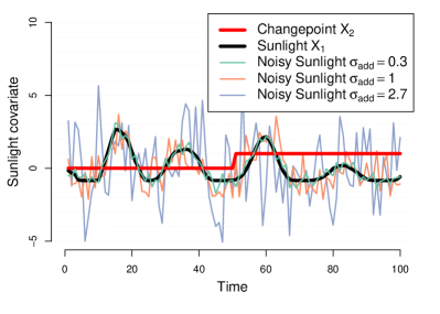
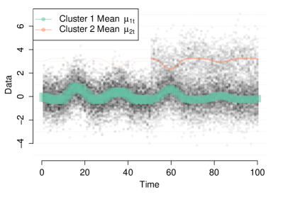
Figure 4: (Left) The thick black line shows the first covariate $\mathbf{\color[rgb]{0,0,0}X}_{1}\in\mathbb{R}^{T}$, which is a smoothed and standardized version of the par (sunlight) covariate from Section 4.0.1. The three thin lines show the obscured sunlight variables for three different noise levels $\sigma_{\text{add}}$. The next covariate is a changepoint variable $\mathbf{\color[rgb]{0,0,0}X}_{2}\in\mathbb{R}^{T}$, shown as a thick red line. The remaining $8$ spurious covariates $\{\mathbf{\color[rgb]{0,0,0}X}_{i}\}_{i=3}^{10}$ are generated as $T$ i.i.d. entries from $\mathcal{N}(0,1+\sigma_{\text{add}}^{2})$; these are not shown here. (Right) An example of a generated dataset, whose particles are shown as grey points in the background. The two true cluster means are plotted as colored lines whose thickness is proportional to the cluster probabilities. Particles for both clusters are generated as $\mathcal{N}(0,1)$ around the cluster means. Cluster $1$ is only present in the second half, and has one quarter of the number of particles in cluster $2$ in those time points. A thin dashed line is shown in the first half where the cluster probability is zero.

On each new synthetic dataset, we estimate a cross-validated $2$-cluster model using radius $r=1.5$, but instead of sunlight covariate $\mathbf{\color[rgb]{0,0,0}X}_{1}$, we use the obscured $\mathbf{\color[rgb]{0,0,0}X}_{1}^{\text{noisy}}=\mathbf{\color[rgb]{0,0,0}X}_{1}+\boldsymbol{\color[rgb]{0,0,0}\epsilon},\boldsymbol{\color[rgb]{0,0,0}\epsilon}\sim\mathcal{N}(0,\sigma_{\text{add}}^{2}\boldsymbol{\color[rgb]{0,0,0}I}_{T})$ for estimation. Also, the eight spurious covariates $\{\mathbf{\color[rgb]{0,0,0}X}_{i}\}_{i=3}^{10}$ are each generated as $\mathcal{N}(0,1+\sigma_{\text{add}}^{2})$ to match the magnitude of $\mathbf{\color[rgb]{0,0,0}X}_{1}^{\text{noisy}}$. We consider a certain range of additive noise $\sigma_{\text{add}}\in\{0,0.3,0.6,\cdots,2.7\}$, and $100$ synthetic datasets for each value $\sigma_{\text{add}}$.

The left plot of Figure 5 shows the out-of-sample model prediction performance of $100$ estimated models for each noise level $\sigma_{\text{add}}$, measured as the negative log likelihood evaluated on a large independent test dataset. As expected, out-of-sample prediction gradually worsens with increasing covariate noise $\sigma_{\text{add}}$, then plateaus at about $\sigma_{\text{add}}=2.7$.

The right plot of Figure 5 demonstrates the variable selection property of our method, focusing on the $\beta$ coefficients. Focusing on the sunlight variable – the only true predictor of mean movement – we see that it is more likely to be selected than are spurious covariates, and is less likely to be selected as $\sigma_{\text{add}}$ increases. Additionally, we see that selecting sunlight is possible even when $\sigma_{\text{add}}$ is high if the cluster has higher relative probability and has nonzero probability in a longer time range.

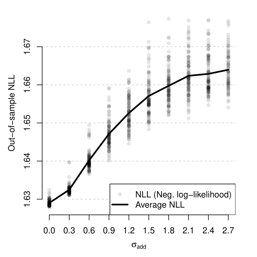
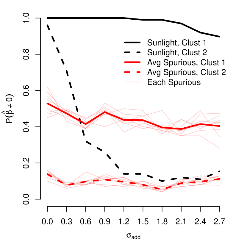
Figure 5: (Left) Out-of-sample prediction performance using covariates obscured by Gaussian noise variance $\sigma_{\text{add}}^{2}$, for the simulation setup described in Section 3.1.1. (Right) The probability of the sunlight covariate (the only relevant covariate for cluster means) being estimated as nonzero is shown in black lines. The corresponding probabilities for the eight spurious covariates are shown in red lines (thin red lines are individual covariates, and the thick red line is the average). The solid and dashed lines show results from cluster 1 and cluster 2 respectively. In both clusters, the sunlight variable is more likely to be selected than the spurious variables. This advantage is more pronounced for cluster $1$ than for cluster $2$, which is only has data in the second half of the time range.

3.1.2 Cluster number misspecification

In addition to covariate noise, we explore the effect of misspecifying the number of clusters $K$ in the model. We first form a ground truth model by taking the five-cluster estimated model from the 1-dimensional $T=296$ data in Section 4.0.1 and Figure 7, and zero-thresholding the smaller estimated coefficients. We then generate new data $30$ times from this underlying true model, and estimate a $K$-cluster cross-validated model, for $K\in\{2,3,4,5,6,7,8\}$. Figure 6 shows out-of-sample prediction performance, measured as the negative log-likelihood on a large independent test set generated from the true model. We see that models estimated with $K<5$ clusters have sharply deteriorating out-of-sample prediction. On the other hand, models estimated with $K>5$ than five clusters have average out-of-sample prediction performance in the same range as that of $K=5$ cluster models. A closer examination of the estimated models reveals that, out of the $K>5$ clusters, five clusters are usually estimated accurately, and the remaining $K-5$ clusters are estimated with near-zero probability. These results suggest that one can slightly overspecify the number of clusters for estimation with little harm to prediction performance. Automatic approaches to choosing $K$ is an interesting area of future work.

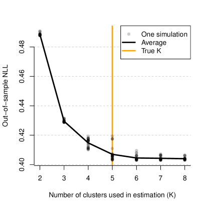
Figure 6: Out-of-sample prediction performance for $K$-cluster models estimated from 5-cluster pseudo-real datasets (which were each generated from a simplified version of a model estimated from real 1-dimensional data, in Section 4.0.1). Models estimated with fewer than $5$ clusters have sharply worse out-of-sample prediction performance. On the other hand, estimated models with $5$ clusters or more have similar out-of-sample prediction performance, because the extra clusters are estimated to have zero probability, and play no role in the prediction.

4 Application to Seaflow cruise

In this section, we apply our model to data collected on a research cruise in the North Pacific Ocean, and from the Simons CMAP database (https://simonscmap.com/). The MGL1704 cruise traversed two oceanographic regions over the course of about 2 weeks, between dates 2017-05-28 and 2017-06-13. As seen in Figure 1, the cruise started in the North Pacific Subtropical Gyre (low latitude, dominated by warm, saltier water), traveling north to the Subpolar Gyre (high latitude, low-temperature, low-salt, nutrient-rich water), and returned back south. We first describe the data and model setup, then discuss the results.

Environmental covariates. A total of 33 environment covariates (see Table 1 and Figure 11 of the Supplement) were colocalized with cytometric data by averaging the environmental data measurements within a rectangle of every discrete point of the cruise trajectory in space and time, aggregated to an hourly resolution. These data were processed and downloaded from the Simons CMAP database (Ashkezari et al., 2021) accessed through the CMAP4R R package (Hyun et al., 2020). In addition to these covariates, we created four new covariates by lagging the sunlight covariate in time by $\{3,6,9,12\}$ hours. This was motivated by scientific evidence showing that the peak of phytoplankton cell division is out of phase with sunlight (Ribalet et al., 2015). We also created two new changepoint variables demarcating the two crossings events of the cruise through a biological transition line at latitude $37\textdegree$. These derived covariates play the role of allowing a more flexible conditional representation of the cytograms, using information from the covariates. All covariates except for the two changepoint variables were centered and scaled to have sample variance of 1. Altogether, we formed a covariate matrix $\mathbf{\color[rgb]{0,0,0}X}\in\mathbb{R}^{(308-12)\times 39}$. (The first twelve time points are deleted due to the the lagging of the sunlight variable.)

Response data (cytograms). The response data (cytograms) were collected on-board using a continuous-time flow cytometer called SeaFlow, which continuously analyzes sea water through a small opening and measures the optical properties of individual microscopic particles (Swalwell et al., 2011). The data consist of measurements of light scatter and fluorescence emissions of individual particles. Data are organized into files recorded every $3$ minutes, where each file contains measurements of the cytometric characteristics of between $1,000$ and $100,000$ particles ranging from $0.5$ to $5$ microns in diameter. The size of data in any given file depends on the cell abundance of phytoplankton within the sampled region. Each particle is characterized by two measures of fluorescence emission (chlorophyll and phycoerythrin), its diameter (estimated from light scatter measurements by the application of Mie theory for spherical particles), its carbon content (cell volume is converted to carbon content) and its label (identified based on a combination of manual gating and a semi-supervised clustering method), as described in Ribalet et al. (2019). Note that we use the particle labels only for comparison to our approach in Section 4.1. Particles were aggregated by hour, resulting in $T=296$ cytograms for the duration of the cruise, with matching time points as rows of $\mathbf{\color[rgb]{0,0,0}X}$.

Lastly, the cytogram data $\{\mathbf{\color[rgb]{0,0,0}y}_{i}^{(t)}\in\mathbb{R}^{3}:i=1,\cdots,n_{t}\}_{t}$ were log transformed due to skewness of the original distributions, augmented with biomass multiplicity $\{C_{i}^{(t)}:i=1,\cdots,n_{t}\}_{t}$, and binned using $D=40$ equally sized bins in each dimension, as described in Section 2.3. In the analyses to follow in Sections 4.0.1 - 4.0.2, we consider two data representations for analysis: a $d=1$ case with only the binned cell diameter biomass cytograms, and the full $d=3$ dimensional binned biomass cytograms.

Practicalities. The regularization parameters $(\lambda_{\alpha},\lambda_{\beta})$ were chosen using 5-fold cross-validation as described in Section 2.6. Every application of the EM algorithm was repeated $5$ times (for 3-dimensional data) or $10$ times (for 1-dimensional example). The model means were restricted using a ball constraint of radius $r$ as described in Section 2.2. In the 1-dimensional data analysis in 4.0.1, the radius reflects the underlying assumption that carbon quotas should at most double or halve, peaking during the day due to carbon fixation via photosynthesis by the cell, and halving due to cell division (i.e. the mother cell divides into two equal daughter cells). Assuming spherical particles, this would correspond to a log scale day-night cell diameter difference of $\log(2)/3\simeq 0.231$, halved to obtain $r=0.1153$. The 3-dimensional data analysis in Section 4.0.2 first shifts and scales the log cell diameter to be in the same range as the other axes, and uses $r=0.5$, which is similar in scale to the radius used in the 1-dimensional analysis.

4.0.1 Application to 1-dimensional cell diameter data

In this section, we apply our model to 1-dimensional cytograms at the hourly time resolution. The 1-dimensional setting is useful for visualization because single plots can display the entire data and fitted model parameters, displaying cluster means $\{\boldsymbol{\color[rgb]{0,0,0}\mu}_{k\cdot}\in\mathbb{R}^{T}\}_{1}^{K}$ as lines and cluster probabilities $\{\pi_{k\cdot}\in\mathbb{R}^{T}\}_{1}^{K}$ as line thickness, as well as shaded approximate 95% conditional density intervals from $\phi(\cdot,\boldsymbol{\color[rgb]{0,0,0}\mu}_{kt},\boldsymbol{\color[rgb]{0,0,0}\Sigma}_{k})$. The estimated means and probabilities are shown in Figure 7, and the estimated coefficients can be seen in Table 2 of the Supplement.

Overall, the estimated model effectively captures the visual patterns in the cytogram data. Clusters $3$ and $5$ correspond to two well-known populations called Synechococcus and Prochlorococcus, respectively. The most prominent phenomenon is the daily fluctuation of the mean of cluster $5$, which is clearly predicted using a combination of time-lagged sunlight and ocean altimetry. Also notable is change in probability of cluster $3$, which is predicted well by physical and chemical covariates such as sea surface temperature and phosphate. The overlapping two clusters $3$ and $4$ are also accurately captured as separate clusters.

As we will see shortly in the 3-dimensional analysis, introducing the other two axes of the cytograms (i.e. 1-dimensional cytograms to 3-dimensional cytograms) clearly helps further distinguish between clusters and identify finer-grain cluster mean movement. Furthermore, cluster $4$, which has a large variance and serves as a catch-all background cluster, does not appear to represent a specific cell population, and rather exists to improve the other clusters’ model fits.

We also estimated the stability of $\beta$ coefficients of this model, by calculating the nonzero proportion of each of the estimated coefficients produced from subsampled datasets. These nonzero proportions are displayed alongside the original coefficient estimates in Tables 7 and 8 in the Supplement, and the entire procedure is detailed in Supplement D. The stability estimates seem quite sensible – they show high nonzero probability of sunlight variables for Prochlorococcus (cluster $5$), as well as overall low nonzero probabilities for the covariates of cluster $4$, the background cluster.

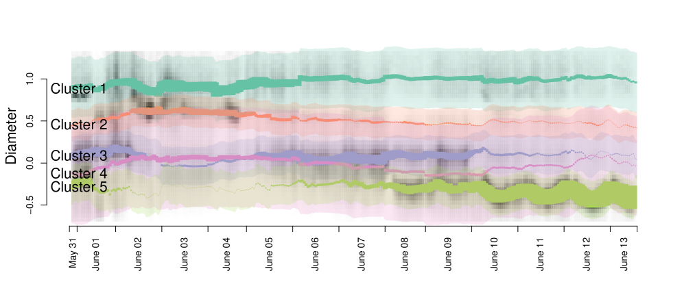
Figure 7: (Top) The 1-dimensional cell diameter biomass cytograms (log transformed) at an hourly time resolution is shown here. In the background, the 1-dimensional biomass distribution of binned cell diameter data is shown in greyscale. (Bottom) The estimated $5$-cluster model is overlaid on the same plot; the five solid lines are the five estimated cluster means, whose thickness show the values of the $K=5$ cluster probabilities $\{\pi_{kt}\}_{k=1}^{K}$ over time $t=1,\cdots,296$ (individual hours). The shaded region around the solid lines are the estimated $\pm 2$ standard deviation around the cluster means.

4.0.2 Application to 3-dimensional data

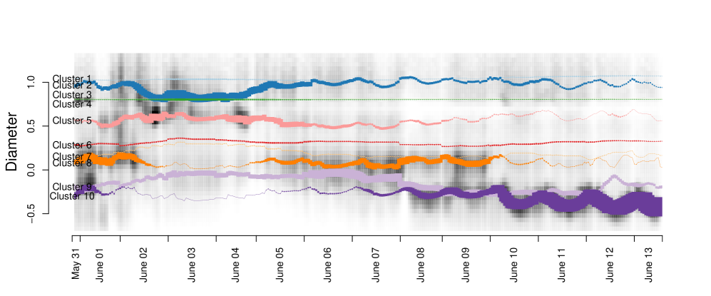
Figure 8: A one-dimensional slice of the estimated model of the full $3$-dimensional data, showing only the cell diameter axis. This figure is directly comparable to Figure 7 using only 1-dimensional cell diameter data. The colored solid lines track the ten estimated cluster means over time, and the line thickness shows the cluster probabilities over time. (The shaded 95% probability regions were omitted for clarity of presentation.) This model on 3-dimensional data suggests finer movement of a larger number of cell populations that is not detectable using only the 1-dimensional data. In particular, a clean separation of the heavily overlapping clusters $9$ and $10$ was not possible in the 1-dimensional model, but is clear in the 3-dimensional model (also see Figure 9 that this separation is made apparent by using the additional red axis).

In this section, we apply our model to the full 3-dimensional data. First, in Figure 8, we display one dimension (cell diameter) of the estimated $10$-cluster $3$-dimensional model, as a direct comparison to the 1-dimensional cell diameter analysis in Section 4.0.1. Cluster $10$ is recognized by domain experts to correspond to Prochlorococcus. The separation of the two heavily overlapping clusters $9$ and $10$, and their independent means’ movement, are visually not apparent in the cell diameter data alone; indeed, the estimated 1-dimensional model in Figure 7 only captures a single Prochlorococcus cluster $5$.

The full $3$-dimensional data and estimated model are challenging to display in print. A better medium than flat images is a video of $t=1,\cdots,T$ images over time, which we show in https://youtu.be/jSxgVvT2wr4. Figure 14 of the Supplement shows one frame from this video (corresponding to one $t$), which overlays with several plots: three $2$-dimensional projections of the cytogram, two different angles of the $3$-dimensional cytograms, the cruise location on a map, the covariates over time, and the cluster probabilities at each time and as a time series. The first four panels of this snapshot are shown in Figure 9 in higher resolution. The mean fluctuations and cluster probability dynamics over time are clearly captured in the full video, and are explained next, in the context of covariates.

The estimated mean movement and the $\beta$ coefficients shown in Tables 4-6 in the Supllement reveal interesting scientific insights. The cell diameter of Prochlorococcus seems to be well predicted by sunlight and lagged variants of sunlight. To elaborate, the estimated entries of $\beta_{5}$ corresponding to the covariates p1, p2 and p3 and the cell diameter axis, were estimated as $0.008$, $0.010$ and $0.013$ – meaning that the mean cell diameters of Prochlorococcus are predicted to increase by these amounts with a unit increase in each covariate value. This supports biochemical intuition about the cell size being directly driven by sunlight. Indeed, important physiological processes of phytoplankton cells, including growth, division, and fluorescence (particularly of the pigment chlorophyll-A), are known to undergo diel variability, i.e. timed with the day-night or light cycle.

Estimated cluster probabilities and the coefficients $\alpha$ shown in Tables 3 are also quite interpretable. A higher positive estimated entry of $\alpha_{k}$ means that a unit increase of that covariate corresponds to a larger increase of the relative probability of the $k$’th cluster. The probability of Cluster $8$ (which occupies a region in the orange fluorescence axis that clearly corresponds to the Synechococcus population) is associated with primary productivity (coefficient value of $0.19$), oxygen ($0.46$) and nitrate ($-0.35$). Rapid increases in the abundance and biomass of Synechococcus associated with high productivity have previously been observed over narrow regions of the Pacific at the boundary between the Subtropical and Subpolar Gyres (Gradoville et al., 2020) . High productivity in the ocean is often linked to high oxygen saturation, a result of oxygen production during photosynthesis, and low nitrate, as a result of consumption of this nutrient required for Synechococcus’s cell growth (Moore et al., 2002). Linkages to such biochemical factors unique to this specific Synechococcus cluster are otherwise difficult to identify, but are clearly identified in our model. In contrast, for cluster $10$ (Prochlorococcus), the largest $\alpha$ coefficients correspond to sea surface temperature ($0.87$) and phosphate ($-0.94$). These results reflect this organism’s observed distribution in the Pacific Ocean; namely its Subtropical Gyre, where high surface temperatures and low concentrations of phosphate tend to favor small-celled Prochlorococcus leading to higher cluster probabilities. Interestingly, nitrate was not detected by the model as a relevant covariate, which is in good agreement with the physiology of Prochlorococcus, which often lack the genes necessary for nitrate assimilation (Berube et al., 2015).

On the other hand, the large positive $\alpha$ coefficients for cluster $2$ (Picoeukaryotes) associated with phosphate ($0.35$) reflects its more northerly distribution in the North Pacific Subpolar Gyre, a region of the ocean distinguished by higher surface concentration of nutrients including phosphate which allow for greater growth of these relatively larger phytoplankton.

Finally, cluster $3$ is particularly interesting as it captures the calibration beads injected by the instrument as an internal standard. The location of this cluster is much more apparent in the full 3-dimensional representation in Figure 9. This is the only population whose origin and location is known a priori, and thus serves as a negative control, which the model is expected to capture. Indeed, in our estimated $10$-cluster 3-dimensional model, this bead is clearly captured as a separate population whose mean movement is minimal over time. Interestingly, 3-dimensional models with fewer than $10$ clusters fail to capture the calibration bead as a separate population.

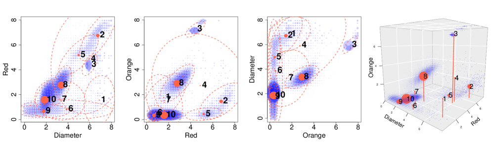
Figure 9: The estimated 3-dimensional 10-cluster model described in Section 4.0.2, at one time point. The size of the blue points represents the biomass in each of the $40^{3}$ bins. The panels show various views of the cytograms – three 2d scatterplots and our estimated parameters (means, probabilities, and covariances). The red dots mark the cluster centers at this time point, and the size (radius) of these red dots are proportional to the cluster probabilities. The red ellipses in dashed lines show the estimated 95% probability region of the data formed from the estimated Gaussian covariance of each cluster. The $10$ estimated model clusters’ mean fluctuations and cluster probability dynamics over time can be seen in the full video in %****␣paper-arxiv.tex␣Line␣1400␣****https://youtu.be/jSxgVvT2wr4 – a single frame of this video is shown in Figure 9.

4.1 Comparison to gating

In Figure 10, we compare the relative biomass of Prochlorococcus, measured in two ways. The dark grey line shows the relative biomass of Prochloroccocus, gated in Ribalet et al. (2019) using flowDensity bioconductor package (Malek et al., 2015), applied semi-automatically to individual 3-dimensional cytograms recorded roughly every $3$ minutes, then aggregated to an hourly level. There is a noticeable discrepancy between the two methods on June 8th and 9th. The dark grey line abruptly rises from near $0$ to about $0.5$, while the purple line follows a gradual increase from June 8th onwards. The reasons for this discrepancy are apparent from visual examination of the gated cytograms. First, the gating results have no continuity or smoothness over time, having been applied to individual cytograms. More importantly, while our model consistently tracks the Prochlorococcus cluster as a single ellipsoidal cluster $10$, the semi-automatic gating function erroneously includes external particles – many from our model’s cluster $9$, which domain experts would not consider to be Prochlorococcus.

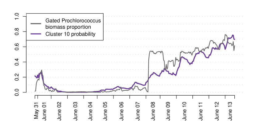
Figure 10: This figure shows the relative biomass of Prochlorococcus, measured in two ways – using traditional gating (black line), and using the estimated cluster probability of cluster $10$ (purple) in the 3-dimensional data in Section 4.0.2 and Figure 9. One noticeable discrepancy is on June 8th and 9th. The gating (black line) abruptly jumps from $0$ to $0.5$ due to flaws in automatic gating, while our model (purple) suggests a gradual increase on June 8th and onwards. Visual inspection and expert annotation of this cluster in the cytogram suggests that our model cluster $10$ is correctly tracking Prochlorococcus.

5 Conclusion

In this work, we propose a novel sparse mixture of multivariate regressions model for modeling flow cytometry data. We devise a penalized expectation-maximization algorithm with parameter constraints and implement a specific ADMM solver, which is called in the M-step. Our simulations and application results in Section 3 and 4 demonstrate that our proposed model can reveal interpretable insights from flow cytometry data, and help scientists identify how environmental conditions influence the dynamics of phytoplankton populations.

Our method provides scientists with a rich description of the association between environmental factors and phytoplankton cell populations. It leverages covariates and all cytograms to identify cell populations. This means two cell populations that might be indistinguishable in a single cytogram could be differentiated if their dynamics (i.e. dependence on covariates) are distinct from each other. Thus, even when one is not interested in the covariates themselves but only the estimation of cell populations (as in gating) this method still may be the best choice. In applying the method, we recover some known associations, such as Prochlorococcus and light (positive controls), we did not identify some known non-associations (negative controls), and also produced some new associations that can be studied. Also, in investigating a discrepancy between our method and a pre-existing gating approach, we uncovered some undesirable behavior of the pre-existing approach, and showcased our method’s ability to perform the difficult task of automatic and consistent gating of overlapping clusters in cytograms over time.

While the motivation from this methodology comes from oceanography, the flow cytometry technology is important to many other areas, including biomarker detection (Gedye et al., 2014), diagnosis of human diseases such as tumors (Brown and Wittwer, 2000), and ecological studies (Props et al., 2016). For instance, in a biomedical application, covariates can be patient attributes, and the response can be cytograms obtained from patient blood samples. In fact, the statistical methodology developed here can be applied to any context in which modeling cytograms in terms of features is reasonable – the time ordering of the data is not required for application. We therefore expect it to be valuable in a wide range of fields.

Our model diagnostics in Supplement E indicate some leftover time dependence in the data residuals from our model. To remedy this within the framework of our model, one might add time-lagged versions of the covariates, or even summaries from cytograms $\mathbf{\color[rgb]{0,0,0}y}^{(t)}$, to directly incorporate time-space autocorrelation in our model. Alternatively, one could also extend the $d$-by-$d$ cluster covariance $\boldsymbol{\color[rgb]{0,0,0}\Sigma}_{k}\in\mathbb{R}^{d\times d}$ to be a time-varying matrix $\boldsymbol{\color[rgb]{0,0,0}\Sigma}_{kt}$. This covariance matrix can take time structure that is not driven by covariates $X^{(t)}$, but has dependence (e.g. time autocorrelation) or smoothness that is learned directly from the data. However, a time series extension also complicates our existing cross-validation strategy for tuning $\lambda_{\alpha}$ and $\lambda_{\beta}$, and constitutes a significant departure from our current proposed model. We view a time-series extension of our model to be an excellent methodology direction to pursue next.

The methodology has several exciting directions for future work. Our mixture model methodology would greatly benefit from a principled, automatic choice of the number of $K$ based on the data. It would be also be interesting to see how relaxing the Gaussian cluster assumption to different distributions – e.g. skewed, multivariate $t$ distributions – helps improve the flexibility of our approach. A model with feature-dependent covariances $\{\boldsymbol{\color[rgb]{0,0,0}\Sigma}_{k}\}_{k=1,\cdots,K}$ could enable more flexible prediction as well. Also promising are the extension and comparison to more non-parametric approaches to the conditional distribution of cytograms, or to the entire joint model of cytograms and environmental covariates.

On the application side, it would be interesting to compare estimated models on data from other oceanographic cruises traversing the same trajectory or different areas, and see to what extent the estimated relationship between cytograms and environmental covariates can be replicated.

References

- Field et al. [1998] Christopher B. Field, Michael J. Behrenfeld, James T. Randerson, and Paul Falkowski. Primary production of the biosphere: Integrating terrestrial and oceanic components. Science, 281(5374):237–240, 1998. ISSN 0036-8075. doi: 10.1126/science.281.5374.237. URL https://science.sciencemag.org/content/281/5374/237.
- Sosik et al. [2010] Heidi M. Sosik, Robert J. Olson, and E. Virginia Armbrust. Flow Cytometry in Phytoplankton Research. In Chlorophyll a Fluorescence in Aquatic Sciences: Methods and Applications, pages 171–185. Springer Netherlands, 2010. doi: 10.1007/978-90-481-9268-7“˙8.
- Dubelaar et al. [1999] George B.J. Dubelaar, Peter L. Gerritzen, Arnout E.R. Beeker, Richard R. Jonker, and Karl Tangen. Design and first results of CytoBuoy: A wireless flow cytometer for in situ analysis of marine and fresh waters. Cytometry, 37(4):247–254, Dec 1999. doi: 10.1002/(sici)1097-0320(19991201)37:4¡247::aid-cyto1¿3.0.co;2-9. URL https://doi.org/10.1002/(sici)1097-0320(19991201)37:4<247::aid-cyto1>3.0.co;2-9.
- Olson et al. [2003] Robert J. Olson, Alexi Shalapyonok, and Heidi M. Sosik. An automated submersible flow cytometer for analyzing pico- and nanophytoplankton: FlowCytobot. Deep Sea Research Part I: Oceanographic Research Papers, 50(2):301–315, Feb 2003. doi: 10.1016/s0967-0637(03)00003-7. URL https://doi.org/10.1016/s0967-0637(03)00003-7.
- Swalwell et al. [2011] Jarred E Swalwell, Francois Ribalet, and E. Virginia Armbrust. Seaflow: A novel underway flow-cytometer for continuous observations of phytoplankton in the ocean. Limnology and Oceanography: Methods, 9(10):466–477, 2011. doi: 10.4319/lom.2011.9.466. URL https://aslopubs.onlinelibrary.wiley.com/doi/abs/10.4319/lom.2011.9.466.
- Vaulot and Marie [1999] D Vaulot and D Marie. Diel variability of photosynthetic picoplankton in the equatorial Pacific. Journal of Geophysical Research. C. Oceans, 104(C2):3297–3310, 1999.
- Sosik et al. [2003] Heidi M Sosik, Robert J Olson, Michael G Neubert, Alexi Shalapyonok, and Andrew R Solow. Growth Rates of Coastal Phytoplankton from Time-Series Measurements with a Submersible Flow Cytometer. Limnology and Oceanography, 48(5):1756–1765, 2003. URL http://www.jstor.org/stable/3597543.
- Ribalet et al. [2015] Francois Ribalet, Jarred Swalwell, Sophie Clayton, Valeria Jiménez, Sebastian Sudek, Yajuan Lin, Zackary I. Johnson, Alexandra Z. Worden, and E. Virginia Armbrust. Light-driven synchrony of Prochlorococcus growth and mortality in the subtropical Pacific gyre. Proceedings of the National Academy of Sciences, 112(26):8008–8012, jun 2015. ISSN 0027-8424. doi: 10.1073/pnas.1424279112. URL http://www.pnas.org/lookup/doi/10.1073/pnas.1424279112.
- Verschoor et al. [2015] Chris P. Verschoor, Alina Lelic, Jonathan L. Bramson, and Dawn M. E. Bowdish. An introduction to automated flow cytometry gating tools and their implementation. Frontiers in Immunology, 6(nil):nil, 2015. doi: 10.3389/fimmu.2015.00380. URL https://doi.org/10.3389/fimmu.2015.00380.
- Hyrkas et al. [2015] Jeremy Hyrkas, Sophie Clayton, Francois Ribalet, Daniel Halperin, E. Virginia Armbrust, and Bill Howe. Scalable clustering algorithms for continuous environmental flow cytometry. Bioinformatics, 32(3):417–423, 10 2015. ISSN 1367-4803. doi: 10.1093/bioinformatics/btv594. URL https://doi.org/10.1093/bioinformatics/btv594.
- Hahne et al. [2009] Florian Hahne, Nolwenn LeMeur, Ryan R Brinkman, Byron Ellis, Perry Haaland, Deepayan Sarkar, Josef Spidlen, Errol Strain, and Robert Gentleman. Flowcore: a bioconductor package for high throughput flow cytometry. BMC Bioinformatics, 10(1):106, 2009. doi: 10.1186/1471-2105-10-106. URL https://doi.org/10.1186/1471-2105-10-106.
- Aghaeepour et al. [2013] Nima Aghaeepour, Greg Finak, FlowCAP Consortium, DREAM Consortium, Holger Hoos, Tim R Mosmann, Ryan Brinkman, Raphael Gottardo, and Richard H Scheuermann. Critical assessment of automated flow cytometry data analysis techniques. Nature methods, 10(3):228–238, March 2013. ISSN 1548-7091. doi: 10.1038/nmeth.2365. URL https://europepmc.org/articles/PMC3906045.
- McLachlan and Peel [2006] G. J. McLachlan and D. Peel. Finite Mixture Models. Wiley, 2006.
- Wang et al. [1996] Peiming Wang, Martin L. Puterman, Iain Cockburn, and Nhu Le. Mixed poisson regression models with covariate dependent rates. Biometrics, 52(2):381, 1996. doi: 10.2307/2532881. URL https://doi.org/10.2307/2532881.
- Khalili and Chen [2007] Abbas Khalili and Jiahua Chen. Variable selection in finite mixture of regression models. Journal of the American Statistical Association, 102(479):1025–1038, 2007. doi: 10.1198/016214507000000590. URL https://doi.org/10.1198/016214507000000590.
- Städler et al. [2010] Nicolas Städler, Peter Bühlmann, and Sara van de Geer. L1-penalization for mixture regression models. TEST, 19(2):209–256, 2010. doi: 10.1007/s11749-010-0197-z. URL https://doi.org/10.1007/s11749-010-0197-z.
- Grün and Leisch [2008] Bettina Grün and Friedrich Leisch. Flexmix version 2: Finite mixtures with concomitant variables and varying and constant parameters. Journal of Statistical Software, Articles, 28(4):1–35, 2008. ISSN 1548-7660. doi: 10.18637/jss.v028.i04. URL https://www.jstatsoft.org/v028/i04.
- Jordan and Jacobs [1993] M.I. Jordan and R.A. Jacobs. Hierarchical mixtures of experts and the em algorithm. In Proceedings of 1993 International Conference on Neural Networks (IJCNN-93-Nagoya, Japan), 1993. doi: 10.1109/ijcnn.1993.716791. URL https://doi.org/10.1109/ijcnn.1993.716791.
- Tibshirani [1996] Robert Tibshirani. Regression shrinkage and selection via the lasso. Journal of the Royal Statistical Society. Series B (Methodological), 58(1):267–288, 1996. ISSN 00359246. doi: 10.2307/2346178. URL http://www.jstor.org/stable/2346178.
- Xu and Jordan [1996] Lei Xu and Michael I. Jordan. On convergence properties of the EM algorithm for gaussian mixtures. Neural Computation, 8(1):129–151, jan 1996. doi: 10.1162/neco.1996.8.1.129. URL https://doi.org/10.1162/neco.1996.8.1.129.
- Marañón [2015] Emilio Marañón. Cell Size as a Key Determinant of Phytoplankton Metabolism and Community Structure. Annual Review of Marine Science, 7(1):241–264, jan 2015. ISSN 1941-1405. doi: 10.1146/annurev-marine-010814-015955. URL http://www.annualreviews.org/doi/10.1146/annurev-marine-010814-015955.
- Pan and Shen [2007] Wei Pan and Xiaotong Shen. Penalized model-based clustering with application to variable selection. Journal of Machine Learning Research, 8:1145–1164, 05 2007.
- Friedman et al. [2010] Jerome Friedman, Trevor Hastie, and Robert Tibshirani. Regularization paths for generalized linear models via coordinate descent. Journal of Statistical Software, 33(1):1–22, 2010. URL http://www.jstatsoft.org/v33/i01/.
- Grant and Boyd [2014] Michael Grant and Stephen Boyd. CVX: Matlab software for disciplined convex programming, version 2.1. http://cvxr.com/cvx, mar 2014.
- Boyd et al. [2011] Stephen Boyd, Neal Parikh, Eric Chu, Borja Peleato, and Jonathan Eckstein. Distributed optimization and statistical learning via the alternating direction method of multipliers. Foundations and Trends® in Machine Learning, 3(1):1–122, 2011. ISSN 1935-8237. doi: 10.1561/2200000016. URL http://dx.doi.org/10.1561/2200000016.
- Boyer et al. [2013] Timothy P. Boyer, John I. Antonov, Olga K. Baranova, Hernan E. Garcia, Daphne R. Johnson, Alexey V. Mishonov, Todd D. O’Brien, Dan Seidov, Smolyar, I. (Igor), Melissa M. Zweng, Christopher R. Paver, Ricardo A. Locarnini, James R. Reagan, Carla Coleman, and Alexandra Grodsky. World ocean database 2013. Database, 2013. doi: 10.7289/V5NZ85MT. URL https://repository.library.noaa.gov/view/noaa/1291.
- Ashkezari et al. [2021] Mohammad D. Ashkezari, Norland R. Hagen, Michael Denholtz, Andrew Neang, Tansy C. Burns, Rhonda L. Morales, Charlotte P. Lee, Christopher N. Hill, and E. Virginia Armbrust. Simons collaborative marine atlas project (simons cmap): an open-source portal to share, visualize and analyze ocean data. bioRxiv, 2021. doi: 10.1101/2021.02.16.431537. URL https://www.biorxiv.org/content/early/2021/02/17/2021.02.16.431537.
- Hyun et al. [2020] Sangwon Hyun, Aditya Mishra, Christian Müller, and Jacob Bien. R package for cmap access, 2020. URL https://github.com/simonscmap/cmap4r. [Online; accessed 19-Dec-2019].
- Ribalet et al. [2019] François Ribalet, Chris Berthiaume, Annette Hynes, Jarred Swalwell, Michael Carlson, Sophie Clayton, Gwenn Hennon, Camille Poirier, Eric Shimabukuro, Angelicque White, and E. Virginia Armbrust. SeaFlow data v1, high-resolution abundance, size and biomass of small phytoplankton in the north pacific. Scientific Data, 6(1), 11 2019. doi: 10.1038/s41597-019-0292-2. URL https://doi.org/10.1038/s41597-019-0292-2.
- Gradoville et al. [2020] Mary R. Gradoville, Hanna Farnelid, Angelicque E. White, Kendra A. Turk‐Kubo, Brittany Stewart, François Ribalet, Sara Ferrón, Paulina Pinedo‐Gonzalez, E. Virginia Armbrust, David M. Karl, Seth John, and Jonathan P. Zehr. Latitudinal constraints on the abundance and activity of the cyanobacterium UCYN‐A and other marine diazotrophs in the North Pacific. Limnology and Oceanography, page lno.11423, mar 2020. doi: 10.1002/lno.11423. URL https://onlinelibrary.wiley.com/doi/abs/10.1002/lno.11423.
- Moore et al. [2002] Lisa R Moore, Anton F Post, Gabrielle Rocap, and Sallie W Chisholm. Utilization of different nitrogen sources by the marine cyanobacteria Prochlorococcus and Synechococcus. Limnology and Oceanography, 47(4):989–996, 2002. ISSN 00243590. doi: 10.4319/lo.2002.47.4.0989.
- Berube et al. [2015] Paul M. Berube, Steven J. Biller, Alyssa G. Kent, Jessie W. Berta-Thompson, Sara E. Roggensack, Kathryn H. Roache-Johnson, Marcia Ackerman, Lisa R. Moore, Joshua D. Meisel, Daniel Sher, Luke R. Thompson, Lisa Campbell, Adam C. Martiny, and Sallie W. Chisholm. Physiology and evolution of nitrate acquisition in Prochlorococcus. The ISME Journal, 9(5):1195–1207, 2015. ISSN 17517370. doi: 10.1038/ismej.2014.211.
- Malek et al. [2015] Mehrnoush Malek, Mohammad Jafar Taghiyar, Lauren Chong, Greg Finak, Raphael Gottardo, and Ryan R Brinkman. flowDensity: reproducing manual gating of flow cytometry data by automated density-based cell population identification. Bioinformatics, 31(4):606–607, feb 2015. ISSN 1367-4803. doi: 10.1093/bioinformatics/btu677. URL http://www.ncbi.nlm.nih.gov/pubmed/25378466https://academic.oup.com/bioinformatics/article-lookup/doi/10.1093/bioinformatics/btu677.
- Gedye et al. [2014] Craig A. Gedye, Ali Hussain, Joshua Paterson, Alannah Smrke, Harleen Saini, Danylo Sirskyj, Keira Pereira, Nazleen Lobo, Jocelyn Stewart, Christopher Go, Jenny Ho, Mauricio Medrano, Elzbieta Hyatt, Julie Yuan, Stevan Lauriault, Maria Kondratyev, Twan van den Beucken, Michael Jewett, Peter Dirks, Cynthia J. Guidos, Jayne Danska, Jean Wang, Bradly Wouters, Benjamin Neel, Robert Rottapel, and Laurie E. Ailles. Cell surface profiling using high-throughput flow cytometry: A platform for biomarker discovery and analysis of cellular heterogeneity. PLoS ONE, 9(8):e105602, 8 2014. doi: 10.1371/journal.pone.0105602. URL https://doi.org/10.1371/journal.pone.0105602.
- Brown and Wittwer [2000] Michael Brown and Carl Wittwer. Flow Cytometry: Principles and Clinical Applications in Hematology. Clinical Chemistry, 46(8):1221–1229, 08 2000. ISSN 0009-9147. doi: 10.1093/clinchem/46.8.1221. URL https://doi.org/10.1093/clinchem/46.8.1221.
- Props et al. [2016] Ruben Props, Pieter Monsieurs, Mohamed Mysara, Lieven Clement, and Nico Boon. Measuring the biodiversity of microbial communities by flow cytometry. Methods in Ecology and Evolution, 7(11):1376–1385, 7 2016. doi: 10.1111/2041-210x.12607. URL https://doi.org/10.1111/2041-210x.12607.