Existence and uniqueness of solution for semi linear conservation laws with velocity field in $L^{\infty}$

Abstract

In this paper we extend results obtained in [3] and [5]. By considering a semi linear conservation law with velocity in $L^{\infty}$, we prove by fixed point arguments existence and uniqueness result and even in a penalized situation.

Souleye Kane

Université Cheikh Anta Diop de Dakar.

Faculty des Sciences et Techniques

S.Fallou Samb

Université Cheikh Anta Diop de Dakar.

Departement de Mathématiques et Informatique

Diaraf Seck

Université Cheikh Anta Diop de Dakar, BP 16889 Dakar Fann,

Ecole Doctorale de Mathématiques et Informatique.

Keywords: transport equations, semi linear PDE, fixed point methods, STILS method, conservation laws, advection-reaction, finite element method, Newton’s method, Picard’s iteration.

1 Introduction

This paper deals about semi linear conservations laws with velocity field in $L^{\infty}.$ Our goal is twofold. On the one hand, the focus is to propose a generalization of space time integrated least square(STILS) method introduced by O. Besson and J. Pousin in [3] for linear conservation laws to semi linear ones. The STILS method has been widely studied in numerous linear cases. Our aim is to introduce a non linearity in the source term and look for theoretical methods to prove existence and uniqueness results. For this, we shall propose methods combining variational and topological methods.
To reach this aim, we shall use two fixed point theorems. The first one is the Banach’s fixed point theorem and the second is due to Schauder. In this latter case, we shall need a penalization argument.
On the other hand, we endeavor to propose numerical methods to analyse semi linear boundary value problems. We shall use finite element methods combined with Picard’s iteration and Newton’s methods.
Finite element method is known to produce spurious oscillations and add diffusions in the orthogonal directions of integral curve when convection-dominated problem is solved see [12] and references therein. To remedy it, the space time integrated least square method has been introduced in finite element context by H. Nguyen and J. Reynen in [9] for solving advection-diffusion equation. And a time marching approach of STILS has been proposed by O. Besson and G. De Montmollin in [2] for solving numerically linear transport equation using the finite element method with $div(u)=0$. To get discrete maximum principle and remove the oscillations produced by the STILS method, J. Pousin, K. Benmansour, E. Bretin and L. Piffet in [5], added to the formulation a constraint of positivity and a penalization of the total variation.
Before presenting the organization of our work, let us point out that interesting works on the SILS method have been already realized. We quote some among them closely related to our theoretical works. In fact, it been has been used by P.Azerad and O. Besson in [1] to give a coercive variational formulation to the transport equation with a free divergence $\mathcal{C}^{1}$ regular velocity vector field. Existence and uniqueness of Space Time Least Square solution of linear conservation law with velocity field in $L^{\infty}$ is proved in [3] by O. Besson and J. Pousin. And in the same paper, these latter deduce a maximum principle result from Stampacchia’s theorem and have established the comparison between the least squares solution and the renormalized solution of these equations.

The paper is organized as follows. In the next section we shall do the presentation of the problem with some useful mathematical tools for our study. The third section is devoted to the existence and uniqueness results. The main used arguments are fixed point theorems (Banach-Picard’s theorem, Schauder’s Theorem). And in the last section, we propose two news numerical methods for computing the solution by using fixed point algorithm.

2 Position of the problem

2.1 Statement of the aim and functional setting

Let $\Omega\subset\mathbb{R}^{d},(d\in\mathbb{N}^{*})$ be a domain with a Lipschitz boundary $\partial\Omega$ satisfying the cone proprety. Let us take $T>0$ , a set $Q=\Omega\times]0,T[$ and consider an advection velocity $u:Q\rightarrow\mathbb{R}^{d}$ with the following regularity property

$$u\in L^{\infty}(Q)^{d}\ \text{with}\ \operatorname{div}(u)\in L^{\infty}(Q).$$

Let $f:\mathbb{R}\longrightarrow\mathbb{R}$ be a function such that $f\in W^{1,\infty}(\mathbb{R}).$ In some situations we can consider $f$ as a $k-$ Lipschitz, for $k$ small enough.

The first question we will look is to find a space time least square solution for the following boundary value problem

$$\left\{\begin{array}[]{l}\frac{\partial c}{\partial t}+\operatorname{div}(uc)=f(c)\text{\ }{in}\ Q\\ c(x,0)=c_{0}(x)\mbox{ in }\Omega\\ c(x,t)=c_{1}(x,t)\ \mbox{on}\ \Gamma_{-}\end{array}\right.$$ (1)

where

$$\Gamma_{-}=\{x\in\partial\Omega:(n(x),u(x,t))<0;\,\,\forall t\in(0,T)\}.$$

and $(.,.)$ is the inner product in $\mathbb{R}^{d}$, $n(x)$ is the outer normal to $\partial\Omega$ at point $x$. For the sake of simplicity one assume that $\Gamma_{-}$ does not depend on the time t.
Let us consider

$$u\in L^{\infty}(Q)^{d}\ \text{such that}\ \operatorname{div}(u)\in L^{\infty}(Q),$$

set $\widetilde{u}=(1,u_{1},u_{2},....,u_{d})$ and $\widetilde{n}(x,t)$ the outer normal to $\partial Q$ at $(x,t)$.

We shall use the notation $\mid E\mid$ to mean the Lebesgue measure of a set $E$ throughout this paper. Let us recall that, the space-time incoming flow boundary is given by

$$\partial Q_{-}=\big{\{}(x,t)\in\partial Q,(\widetilde{u}(x,t),\widetilde{n}(x,t))<0\big{\}}=\Omega\times\{0\}\cup\Gamma_{-}\times]0,T[.$$

The incoming flow boundary condition in space-time is defined as follows

$$c_{b}(x,t)=\left\{\begin{array}[]{l}c_{0}(x)\mbox{ if }t=0\\ c_{1}(x,t)\ \mbox{on}\ \Gamma_{-}\end{array}\right.$$

We introduce the following norm defined by:

1. $\|\phi\|^{2}=\|\phi\|_{L^{2}(Q)}^{2}+\|\widetilde{div}(\widetilde{u}\phi)\|_{L^{2}(Q)}^{2}-\displaystyle\int_{\partial Q_{-}}\phi^{2}(\widetilde{u},\widetilde{n})\mathrm{d}s$ for all $\phi\in D(\overline{Q}).$
   Where

2. $\,\,\,\,\,\,\widetilde{\nabla}\phi=(\frac{\partial\phi}{\partial t},\frac{\partial\phi}{\partial x_{1}},\frac{\partial\phi}{\partial x_{1}},..,\frac{\partial\phi}{\partial x_{d}});$

3. $\,\,\,\,\,\,\widetilde{\operatorname{div}}(\widetilde{u}\phi)=\frac{\partial\phi}{\partial t}+\displaystyle\sum_{i=1}^{d}\frac{\partial(\phi u)}{\partial x_{i}};$

4. And the Sobolev space $H(u,Q)=\overline{D(\overline{Q})}^{\|.\|};$

5. Note that if $u$ is regular enough for instance $u\in L^{\infty}(Q)^{d}\ \text{with}\ \operatorname{div}(u)\in L^{\infty}(Q),$ then $\,\,\,\,\,\,H(u,Q)\cap L^{\infty}=\big{\{}\phi\in L^{2}(Q);\widetilde{\operatorname{div}}(\widetilde{u}\phi)\in L^{2}(Q),\phi_{/\partial Q_{-}}\in L^{2}(\partial Q_{-};\mid(\widetilde{u},\widetilde{n})\mid)\}\cap L^{\infty}$ for more details see [3].

Before proceeding further, let us remind the following theorems that will be useful for our work and for their proofs, we invite the reader to see [3].

Theorem 2.1

Let us consider $u\in L^{\infty}(Q)^{d}\ \text{with}\ \operatorname{div}(u)\in L^{\infty}(Q)$.Then the normal trace of u $(\widetilde{u},\widetilde{n})\in L^{\infty}(\partial Q).$

Theorem 2.2

Let $u\in L^{\infty}(Q)^{d}\ \text{with}\ \operatorname{div}(u)\in L^{\infty}(Q)$. Then there exists a linear continuous trace operator

$$\begin{array}[]{clcl}\gamma_{\widetilde{n}}:&H(u,Q)&\longrightarrow&L^{2}(\partial Q;(\widetilde{u},\widetilde{n}))\\ &\phi&\longmapsto&\phi_{/\partial Q}\\ \end{array}$$

which can be localized as

$$\begin{array}[]{clcl}\gamma_{\widetilde{n}\pm}:&H(u,Q)&\longrightarrow&L^{2}(\partial Q_{\pm};(\widetilde{u},\widetilde{n}))\\ &\phi&\longmapsto&\phi_{/\partial Q_{\pm}}.\end{array}$$

Finally, let us define the spaces

$$H_{0}(u,Q,\partial Q_{-})=\big{\{}\phi\in H(u,Q),\phi=0\ \text{on }\ \partial Q_{-}\big{\}}=H(u,Q)\cap Ker\gamma_{\widetilde{n}_{-}}$$

and

$$G_{\pm}=\gamma_{\widetilde{n}_{\pm}}(H(u,Q)).$$

Let us give the curved inequality still called curved Poincaré inequality, below that is fundamental and even is the precursor of existence of STILS solution. It has been introduced and proved in [1] for free-divergence and extended in [3].
There exists $c_{p}>0$ such that for any $\phi\in H(u,Q):$

$$\|\phi\|_{L^{2}(Q)}^{2}\leq c_{p}^{2}\big{(}\|\widetilde{\operatorname{div}}(\widetilde{u}\phi)\|_{L^{2}(Q)}^{2}-\int_{\partial Q_{-}}\phi^{2}(\widetilde{u},\widetilde{n})\mathrm{d}s\big{)}$$ (2)

From the curved inequality one deduces the following theorem.

Theorem 2.3

Let $u\in L^{\infty}(Q)^{d}\ \text{with}\ \operatorname{div}(u)\in L^{\infty}(Q)$.Then the semi norm on $H(u,Q)$ defined by

$$\mid\phi\mid_{1,u}^{2}=\|\widetilde{\operatorname{div}}(\widetilde{u}\phi)\|_{L^{2}(Q)}^{2}-\int_{\partial Q_{-}}\phi^{2}(\widetilde{u},\widetilde{n})\mathrm{d}s$$

is a square of norm, equivalent to the norm defined on $H(u,Q).$

Thus $H(u,Q)$ can be equipped by the norm $\mid.\mid_{1,u}.$

Remark 2.1

In the free-divergence case, one gets that $c_{p}\leq 2T$ (see for instance [1] for additional information).

2.2 Space time least square and the linear problem

In this section, we are going to recall the design and some proprieties of STILS method for solving the following linear conservation laws problem.

$$\left\{\begin{array}[]{l}\frac{\partial c}{\partial t}+\operatorname{div}(uc)=f\text{\ }{in}\ Q\\ c(x,0)=c_{0}(x)\mbox{ in }\Omega\\ c(x,t)=c_{1}(x,t)\ \mbox{on}\ \Gamma_{-}.\end{array}\right.$$ (3)

The space time least square solution of (3) corresponds to a minimizer in

$$\big{\{}\phi\in H(u,Q);\gamma_{\widetilde{n}_{-}}(\phi)=c_{b}\big{\}}$$

of the following convex, $H(u,Q)$-coercive functional defined by

$$J(c)=\dfrac{1}{2}\big{(}\int_{Q}(\widetilde{\operatorname{div}}(\widetilde{u}c)-f)^{2}\mathrm{d}x\mathrm{d}t-\int_{\partial Q_{-}}c^{2}(\widetilde{u},\widetilde{n})\mathrm{d}s\big{)}$$ (4)

The Gâteaux-differential of J yields

$$D[J(c)].\phi=\int_{Q}(\widetilde{\operatorname{div}}(\widetilde{u}c)-f)\widetilde{\operatorname{div}}(\widetilde{u}\phi)\mathrm{d}x\mathrm{d}t-\int_{\partial Q_{-}}c\phi(\widetilde{u},\widetilde{n})\mathrm{d}s.$$ (5)

Thus, if $c_{b}\in G_{-}$, the space time last square formulation of (3) is expressed as follows

$$\int_{Q}\widetilde{\operatorname{div}}(\widetilde{u}c)\widetilde{\operatorname{div}}(\widetilde{u}\phi)\mathrm{d}x\mathrm{d}t=\int_{Q}f\widetilde{\operatorname{div}}(\widetilde{u}\phi)\mathrm{d}x\mathrm{d}t\,\,\forall\,\,\phi\in H_{0}(u,Q)$$ (6)

and

$$\gamma_{\widetilde{n}_{-}}(c)=c_{b}.$$

For more details see [3], [5].

Thanks to Theorem 2.2 we can reduce the problem (6) in a homogeneous one in $\partial Q_{-}.$ For $c_{b}\in G_{-}$, let $C_{b}\in H(u,Q)$ such that $\gamma_{\widetilde{n}_{-}}(C_{b})=c_{b}$ then $\rho=c-C_{b}$ is the unique solution of

$$\int_{Q}\widetilde{\operatorname{div}}(\widetilde{u}\rho)\widetilde{\operatorname{div}}(\widetilde{u}\phi)\mathrm{d}x\mathrm{d}t=\int_{Q}(f-\widetilde{\operatorname{div}}(\widetilde{u}C_{b}))\widetilde{\operatorname{div}}(\widetilde{u}\phi)\mathrm{d}x\mathrm{d}t\,\,\forall\,\,\phi\in H_{0}(u,Q).$$ (7)

Finally let us recall the following theorem proved in [3].

Theorem 2.4

For $u\in L^{\infty}(Q)^{d}\ \text{with}\ \operatorname{div}(u)\in L^{\infty}(Q)$, $c_{b}\in G_{-}$, and $f\in L^{2}(Q)$, the problem (7) has a unique solution. Moreover

$$\mid\rho\mid_{1,u}\leq\|f\|_{L^{2}(Q)}+\|\widetilde{\operatorname{div}}(\widetilde{u}C_{b})\|_{L^{2}(Q)}$$

and the function $c=\rho+C_{b}$ is the espace-time least squares solution of (3).

2.3 Space time least square and semi linear problem

This last subsection is devoted to introduce a variational formulation (1). Otherwise our aim is to find $c\in H(u,Q)$ such that

$$\int_{Q}\widetilde{\operatorname{div}}(\widetilde{u}c)\widetilde{\operatorname{div}}(\widetilde{u}\phi)\mathrm{d}x\mathrm{d}t=\int_{Q}f(c)\widetilde{\operatorname{div}}(\widetilde{u}\phi)\mathrm{d}x\mathrm{d}t\,\,\forall\,\,\phi\in H_{0}(u,Q,\partial Q_{-})$$ (8)

and

$$\gamma_{\widetilde{n}_{-}}(c)=c_{b}$$ (9)

It is important to stress that the above formulation is nonlinear. And we shall propose fixed point methods to study it. Let us recall that there are at least three distinct classes of such abstract theorems that are useful for proving existence results in a wide family of partial differential equations. These classes are

• fixed point theorems for strict contractions,

• fixed point theorems for compact mappings and

• fixed point theorems for order preserving operators.

We shall use in the following the two first types.

3 Existence and qualitative results

3.1 Existence and uniqueness

In this section we shall study the problem (8) by establishing and proving existence and uniqueness theorems for the STILS solution. Theses results are deduced thanks to the fixed point theory namely the Banach-Picard and Schauder theorems.

At first, in the case where $f$ is $k-$ Lipschitz with $k$ is small enough that will be precised and by using the Banach-Picard fixed point theorem ([4] ), we have the following existence and uniqueness theorem of STILS solution.

Theorem 3.1

Let $u\in L^{\infty}(Q)$ with $\operatorname{div}(u)\in L^{\infty}(Q)$ , and $c_{b}\in G_{-}$ , $f$ be $k-$ Lipschitz in $\mathbb{R}$ with $k<\frac{1}{c_{p}}$. Then the problem (8)-(9) has a unique solution.

Proof.

Let us consider

$$\mathbb{H}=\big{\{}\phi\in H(u,Q),\gamma_{\widetilde{n}_{-}}(\phi)=c_{b}\big{\}}$$

For all $\rho\in\mathbb{H}$ ,$f(\rho)\in L^{2}(Q)$ then, by 2.4, there exists a unique element $c\in\mathbb{H}$ satisfying :

$$\int_{Q}\widetilde{\operatorname{div}}(\widetilde{u}c)\widetilde{\operatorname{div}}(\widetilde{u}\phi)\mathrm{d}x\mathrm{d}t=\int_{Q}f(\rho)\widetilde{\operatorname{div}}(\widetilde{u}\phi)\mathrm{d}x\mathrm{d}t$$ (10)

for all $\phi\in H_{0}(u,Q,\partial Q_{-})$

Let us define,

$$T:\mathbb{H}\rightarrow\mathbb{H}$$ (11)

such that

$$T(\rho)=c$$ (12)

thus a solution of the non linear problem (8-9) is a fixed point of T.
Let $\rho_{1}$ , $\rho_{2}$ $\in$ $\mathbb{H}$ and $c_{1}=T(\rho_{1})$, $c_{2}=(T\rho_{2}).$
Since $c_{1}-c_{2}=0$ on $\partial Q_{-}$

$$\mid c_{1}-c_{2}\mid^{2}_{1,u}=\|\widetilde{\operatorname{div}}(\widetilde{u}(c_{1}-c_{2}))\|_{L^{2}(Q)}^{2}=\int_{Q}\widetilde{\operatorname{div}}(\widetilde{u}(c_{1}-c_{2}))\widetilde{div}(\widetilde{u}(c_{1}))\mathrm{d}x\mathrm{d}t-\int_{Q}\widetilde{div}(\widetilde{u}(c_{1}-c_{2}))\widetilde{\operatorname{div}}(\widetilde{u}(c_{2}))\mathrm{d}x\mathrm{d}t.$$

For $c_{1}=T(\rho_{1})$ and $c_{2}=T(\rho_{2})$ we have

$$\int_{Q}\widetilde{\operatorname{div}}(\widetilde{u}c_{1})\widetilde{\operatorname{div}}(\widetilde{u}(c_{1}-c_{2}))\mathrm{d}x\mathrm{d}t=\int_{Q}f(\rho_{1})\widetilde{\operatorname{div}}(\widetilde{u}(c_{1}-c_{2}))\mathrm{d}x\mathrm{d}t$$

and

$$\int_{Q}\widetilde{\operatorname{div}}(\widetilde{u}c_{2})\widetilde{\operatorname{div}}(\widetilde{u}(c_{1}-c_{2}))\mathrm{d}x\mathrm{d}t=\int_{Q}f(\rho_{2})\widetilde{\operatorname{div}}(\widetilde{u}(c_{1}-c_{2}))\mathrm{d}x\mathrm{d}t.$$

Then a computation yields

$$\mid c_{1}-c_{2}\mid^{2}_{1,u}=\int_{Q}f(\rho_{1})\widetilde{\operatorname{div}}(\widetilde{u}(c_{1}-c_{2}))\mathrm{d}x\mathrm{d}t-\int_{Q}\ f(\rho_{2})\widetilde{\operatorname{div}}(\widetilde{u}(c_{1}-c_{2}))\mathrm{d}x\mathrm{d}t.$$

$$\mid c_{1}-c_{2}\mid^{2}_{1,u}=\int_{Q}(f(\rho_{1})-f(\rho_{2}))\widetilde{\operatorname{div}}(\widetilde{u}(c_{1}-c_{2}))\mathrm{d}x\mathrm{d}t$$

By Young’s inequality, we get:

$$\mid c_{1}-c_{2}\mid^{2}_{1,u}\leq\|f(\rho_{1})-f(\rho_{2})\|_{{L^{2}(Q)}}\|\widetilde{\operatorname{div}}(\widetilde{u}(c_{1}-c_{2}))\|_{{L^{2}(Q)}}$$

Since $f$ is $k-$ Lipschitz in $\mathbb{R}$ and $\mid c_{1}-c_{2}\mid_{1,u}=\|\widetilde{div}(\widetilde{u}(c_{1}-c_{2}))\|_{{L^{2}(Q)}}$ we have:

$$\mid c_{1}-c_{2}\mid_{1,u}^{2}\leq k\|\rho_{1}-\rho_{2}\|_{{L^{2}(Q)}}^{2}\mid c_{1}-c_{2}\mid_{1,u}$$

and hence

$$\mid c_{1}-c_{2}\mid^{2}_{1,u}\leq kc_{p}\mid\rho_{1}-\rho_{2}\mid_{1,u}\mid c_{1}-c_{2}\mid_{1,u}.$$

Finally we get

$$\mid T(\rho_{1})-T(\rho_{2})\mid_{1,u}\leq kc_{p}\mid\rho_{1}-\rho_{2}\mid_{1,u}.$$

Thus T is a strict contraction, provided that $kc_{p}<1.$ The Banach’s fixed point theorem ensures the existence and uniqueness of $c\in\mathbb{H}$ with $T(c)=c$ which solves (8)-(9) ∎

Remark 3.1

In the free-divergence case, the previous assumption gives $k<\frac{1}{2T}$ thus we get a solution for small times. But it can not be extended because of the lost of continuity.
The constant $c_{p}$ is not optimal (see [3] for more details). And so, the condition $kc_{p}<1$ could be improved.

Now, let us state and prove the following technical lemmas that will be key steps in the building of the next existence theorem.

Lemma 3.2

There is a positive constant $C>0$ such that for any $\phi\in D(\overline{Q})\,\,\text{verifying }\,\,\phi=0\,\,\text{on }\partial Q_{-}$, we have $\|\widetilde{\nabla}\phi\|_{L^{2}(Q)^{d+1}}\leq C\|\widetilde{\operatorname{div}}(\widetilde{u}\phi)\|_{L^{2}(Q)}$

Proof.

Let us suppose that the inequality is false. Then for any integer $n\in\mathbb{N}$, there is $\phi_{n}\in D(\overline{Q})$ tuch that :

$$\|\widetilde{\nabla}\phi_{n}\|_{L^{2}(Q)^{d+1}}>n\|\widetilde{\operatorname{div}}(\widetilde{u}\phi_{n})\|_{L^{2}(Q)}$$ (13)

If $n$ is such that $\|\widetilde{\nabla}\phi_{n}\|_{L^{2}(Q)^{d+1}}=0$ then $\|\widetilde{\nabla}\phi_{n}\|_{L^{2}(Q)^{d+1}}=n\|\widetilde{\operatorname{div}}(\widetilde{u}\phi_{n})\|_{L^{2}(Q)}=0$ which is a contradiction with (13).
Now dividing (13) by $\|\widetilde{\nabla}\phi_{n}\|_{L^{2}(Q)^{d+1}}$, we have :

$$\|\widetilde{\nabla}\frac{\phi_{n}}{\|\widetilde{\nabla}\phi_{n}\|}\|_{L^{2}(Q)^{d+1}}>n\|\widetilde{\operatorname{div}}(\widetilde{u}\frac{\phi_{n}}{\|\widetilde{\nabla}\phi_{n}\|})\|_{L^{2}(Q)}$$ (14)

Setting $\theta_{n}=\frac{\phi_{n}}{\|\widetilde{\nabla}\phi_{n}\|_{L^{2}(Q)^{d+1}}}$, we obtain :

$$\|\widetilde{\nabla}\theta_{n}\|_{L^{2}(Q)^{d+1}}=1$$ (15)

and

$$\|\widetilde{\operatorname{div}}(\widetilde{u}\theta_{n})\|_{L^{2}(Q)}=\|\widetilde{\operatorname{div}}(\widetilde{u}\frac{\phi_{n}}{\|\widetilde{\nabla}\phi_{n}\|})\|_{L^{2}(Q)}.$$ (16)

Thanks to (15) and (16), the inequality (14) can be written as follows

$$\|\widetilde{\operatorname{div}}(\widetilde{u}\theta_{n})\|_{L^{2}(Q)}<\frac{1}{n}.$$ (17)

By curved inequality (also named curved Poincaré inequality) we get existence of a positive constant $A>0$ such that :

$$\|\theta_{n}\|_{L^{2}(Q)}\leq\sqrt{A}\|\widetilde{\operatorname{div}}(\widetilde{u}\theta_{n})\|_{L^{2}(Q)},$$

then

$$\|\theta_{n}\|_{L^{2}(Q)}\leq\frac{\sqrt{A}}{n}.$$ (18)

This implies that :

$$\theta_{n}\longrightarrow 0\,\,\mbox{in}\,\,L^{2}(Q).$$ (19)

From (15) and (18) one deduces that $(\theta_{n})$ is bounded in $H^{1}(Q).$ Then there is a convex combination of the sequence $(\theta_{n})$ that converges to $\theta^{*}\in H^{1}(Q)$ weakly, and so in $L^{2}(Q)$ too. Using (19), this convex combination converges to $0$ in $L^{2}(Q)$. Thanks to the uniqueness of the limit we have $\theta^{*}=0$.
As a sum up, one sees that (13) yields existence of a sequence $(\theta_{n})_{n}\subset D(\overline{Q})\subset H^{1}(Q)$ satisfying:

$$\left\{\begin{array}[]{l}\theta_{n}\longrightarrow 0\,\,\mbox{weakly in }\,\,H^{1}(Q)\,\,(i)\\ \|\widetilde{\nabla}\theta_{n}\|_{L^{2}(Q)^{d+1}}=1\,\,\mbox{for any}\,\,n\in\mathbb{N}\,\,(ii)\end{array}\right.$$ (20)

(i) implies that $\widetilde{\nabla}\theta_{n}\longrightarrow 0\,\,\mbox{weakly in }\,\,L^{2}(Q).$
Let $\psi\in L^{2}(Q)^{d+1}$ such that $\|\psi\|_{L^{2}(Q)^{d+1}}=1.$
We have : $(\psi,\widetilde{\nabla}\theta_{n})\longrightarrow 0\,\,\mbox{in}\,\,\mathbb{R}$.
The translation of the definition of the limit allows us to write:
$\exists n_{0}\in\mathbb{N}$ such that for any $n\geq n_{0}$, we have $\mid(\psi,\widetilde{\nabla}\theta_{n})\mid<1$.
Thus we get $\underset{\|\psi\|_{L^{2}(Q)^{d+1}}=1}{\text{Sup }}\mid(\psi,\widetilde{\nabla}\theta_{n})\mid<1$.
Hence, one deduces that $\|\widetilde{\nabla}\theta_{n}\|_{L^{2}(Q)^{d+1}}<1$ for any $n\geq n_{0}:$ what is in contradiction with (ii). ∎

Lemma 3.3

Let $f:\mathbb{R}\longrightarrow\mathbb{R}$ be a $k$ -Lipschitzian function.
For any $\rho\in H(u,Q),$we have $f(\rho)\in H^{1}(Q).$ In addition there exists a positive $C>0$ such that

$$\|\widetilde{\nabla}f(\rho)\|_{L^{2}(Q)^{d+1}}\leq C\|\widetilde{\operatorname{div}}(\widetilde{u}\rho)\|_{L^{2}(Q)}$$

Proof.

Let $\rho\in H(u,Q)$, then there is a sequence $(\rho_{n})\subset D(\overline{Q})$ that converges to $\rho$ in $H(u,Q)$.
Since $f$ is $k$ -Lipschitzian, we get:
$\mid f(\rho_{n})\mid\leq k\mid\rho_{n}\mid+\mid f(0)\mid$ and $\mid f(\rho)\mid\leq k\mid\rho\mid+\mid f(0)\mid$.
Therefore $(f(\rho_{n}))\subset L^{2}(Q)$ and $f(\rho)\in L^{2}(Q)$. In addition: $\|f(\rho_{n})-f(\rho)\|_{L^{2}(Q)}\leq k\|\rho_{n}-\rho\|_{L^{2}(Q)}$ and $\rho_{n}$ converges to $\rho$ in $L^{2}$ thus $f(\rho_{n})$ converges to $f(\rho)$ in $L^{2}.$ And in particular any convex combination of $f(\rho_{n})$ converges to $f(\rho)$ in $L^{2}.$

Now let us take , $x,y$ in $Q$ .

$$\mid f(\rho_{n}(x))-f(\rho_{n}(y))\mid\leq k\mid\rho_{n}(x)-\rho_{n}(y)\mid$$ (21)

$$\mid f(\rho_{n}(x))-f(\rho_{n}(y))\mid\leq k\mid\nabla\rho_{n}\mid_{\infty}\mid x-y\mid.$$

Under Rademacher’s theorem, for any integer $n$, the function $f(\rho_{n})$ is differentiable almost everywhere and there is a positive constant depending on $n,$ $C_{n}$ such that $\mid\frac{\partial f(\rho_{n})}{\partial x_{i}}\mid\leq C_{n};$ and then $\frac{\partial f(\rho_{n})}{\partial x_{i}}\in L^{2}(Q)\,\,\mbox{for any }\,\,i=1,...,d+1$ .
Using again the inequality (21), one sees that :

$$\mid\frac{\partial f(\rho_{n})}{\partial x_{i}}\mid\leq k\mid\frac{\partial\rho_{n}}{\partial x_{i}}\mid\,\,\mbox{for any }\,\,i=1,...,d+1$$

and then

$$\|\widetilde{\nabla}f(\rho_{n})\|_{L^{2}(Q)^{d+1}}\leq k\|\widetilde{\nabla}\rho_{n}\|_{L^{2}(Q)^{d+1}}.$$

By Lemma 3.2, we have $\|\widetilde{\nabla}\rho_{n}\|_{L^{2}(Q)^{d+1}}\leq C\|\widetilde{\operatorname{div}}(\widetilde{u}\rho_{n})\|_{L^{2}(Q)}$.
This yields

$$\|\widetilde{\nabla}f(\rho_{n})\|_{L^{2}(Q)^{d+1}}\leq kC\|\widetilde{\operatorname{div}}(\widetilde{u}\rho_{n})\|_{L^{2}(Q)}.$$ (22)

Since $(\rho_{n})$ convergs to $\rho$ in $H(u,Q)$ we get $\|\widetilde{\operatorname{div}}(\widetilde{u}\rho_{n})\|_{L^{2}(Q)}$ converges to $\|\widetilde{\operatorname{div}}(\widetilde{u}\rho)\|_{L^{2}(Q)}.$ And we can conclude that $(f(\rho_{n}))$ is bounded in $H^{1}(Q)$.
And more, we have $(f(\rho_{n}))$ is bounded in $H^{1}(Q).$ Then there is $\theta\in H^{1}(Q)$ such that $(f(\rho_{n}))$ converges to $\theta$ weakly. Thanks to Mazur’s lemma, there is a convex combination of the sequence $(f(\rho_{n}))$,denoted $\theta_{n}$ that strongly converges to $\theta$ in $H^{1}(Q)$and then in $L^{2}.$ And the same convex combination converges to $f(\rho)$ in $L^{2}(Q)$ .
Under uniqueness in $L^{2}(Q)$, we have $f(\rho)=\theta$ but $\theta\in H^{1}(Q)$. This ensures us that $f(\rho)\in H^{1}(Q)$.
Passing to the limit the inequality (22), yields

$$\|\widetilde{\nabla}f(\rho)\|_{L^{2}(Q)^{d+1}}\leq kC\|\widetilde{\operatorname{div}}(\widetilde{u}\rho)\|_{L^{2}(Q)}$$

∎

Lemma 3.4

Let $f:\mathbb{R}\longrightarrow\mathbb{R}$ be a $k$ -Lipschitzian function, $C$ be a bounded subset of $H(u,Q)$ and $(\rho_{n})$, $(c_{n})$ be sequences in $C.$ Denoting by $c$ the weak limit of $(c_{n})$ in $H_{0}(u,Q).$ We have :

$$\int_{Q}f(\rho_{n})\widetilde{\operatorname{div}}(\widetilde{u}(c_{n}-c))\mathrm{d}x\mathrm{d}t\longrightarrow 0.$$

Proof.

Since $C\subset H(u,Q)$, $(\rho_{n})$, $(c_{n})$ are sequences of $C$, there are $M>0$ and $c\in H(u,Q)$ such that

$$\|\widetilde{\operatorname{div}}(\widetilde{u}\rho_{n})\|_{L^{2}(Q)}\leq M$$ (23)

and

$$c_{n}\rightharpoonup c\,\,\text{faiblement \,\,dans }H(u,Q)$$ (24)

Using the curved Poincaré inequaity, (23) we have

$$\|\rho_{n}\|_{L^{2}(Q)}\leq M\sqrt{A}$$ (25)

$$\mid f(\rho_{n})\mid\leq k\mid\rho_{n}\mid+\mid f(0)\mid.$$ (26)

Thus (25-26)yield a constant $C_{\ref{fin5}}$ such that :

$$\|f(\rho_{n})\|_{L^{2}(Q)}\leq C_{\ref{fin5}}.$$ (27)

In another way, by Lemma3.3, there exists a constant $C>0$ such that

$$\|\widetilde{\nabla}f(\rho_{n})\|_{L^{2}(Q)^{d+1}}\leq C\|\widetilde{\operatorname{div}}(\widetilde{u}\rho_{n})\|_{L^{2}(Q)}.$$ (28)

From (23)and (28) we have the following estimation

$$\|\widetilde{\nabla}f(\rho_{n})\|_{L^{2}(Q)^{d+1}}\leq CM.$$ (29)

Relations (27) et (29) imply that the sequence $(f(\rho_{n}))$ is bounded in $H^{1}(Q).$ Then, by Rellich’s theorem, even if it means extracting a subsequence, there is $F\in L^{2}(Q)$ such that

$$f(\rho_{n})\longrightarrow F\,\,\mbox{strongly \,\,in }L^{2}(Q).$$ (30)

From (24) and (30), we get

$$\langle f(\rho_{n}),\widetilde{\operatorname{div}}(\widetilde{u}(c_{n}-c))\rangle\longrightarrow(F,0)=0.$$ (31)

Finally we have

$$\int_{Q}f(\rho_{n})\widetilde{\operatorname{div}}(\widetilde{u}(c_{n}-c))\mathrm{d}x\mathrm{d}t\longrightarrow 0.$$

∎

Having at hands these lemmas and using fixed Schauder’s theorem, we can proceed further to get existence and uniqueness results.

Theorem 3.5

Let $u\in L^{\infty}(Q)$ with $\operatorname{div}(u)\in L^{\infty}(Q)$, and $c_{b}\in G_{-},$ $f\in W^{1,\infty}(\mathbb{R}).$ Then the problem (8)-(9) has a solution in $H_{0}(u,Q,\partial Q_{-})$.

Proof.

Since $c_{b}\in G_{-}$ changing the source term if necessary, we shall assume that $c_{b}=0\,\text{on}\,\partial Q_{-}$.
Existence.
The proof is relied mainly on the Schauder’s fixed theorem.
Step 1: we first have to choose a bounded subset $\mathbb{X}$ of $H_{0}(u,Q,\partial Q_{-})$ and a mapping $T:\mathbb{X}\rightarrow\mathbb{X}$. To achieve this aim, for all $\rho\in V$, under the Lemma3.3, or since $f\in W^{1,\infty}(\mathbb{R})$ we have $f(\rho)\in L^{2}(Q).$ Then by Theorem 2.4 there exists a function $c\in H_{0}(u,Q,\partial Q_{-})$ such that

$$\int_{Q}\widetilde{\operatorname{div}}(\widetilde{u}c)\widetilde{\operatorname{div}}(\widetilde{u}\phi)\mathrm{d}x\mathrm{d}t=\int_{Q}f(\rho)\widetilde{\operatorname{div}}(\widetilde{u}\phi)\mathrm{d}x\mathrm{d}t\,\,\text{for all }\,\phi\in H_{0}(u,Q,\partial Q_{-}).$$

Moreover $\mid c\mid_{1,v}\leq\|f(\rho)\|_{L^{2}(Q)}.$
Since $f\in W^{1,\infty}(\mathbb{R})$, we have $\mid c\mid_{1,u}\leq\mid f\mid_{L^{\infty}}\mid Q\mid^{\frac{1}{2}}.$

Let us define, $T:H_{0}(u,Q,\partial Q_{-})\rightarrow H_{0}(u,Q,\partial Q_{-})$ such that $c=T(\rho)$.
Solving (39) is equivalent to show the existence of fixed point theorem of T.
Let us proceed further and choose a convex set $\mathbb{X}$ as follows :

$$\mathbb{X}=\{\phi\in H_{0}(u,Q,\partial Q_{-}),\mid\phi\mid_{1,u}\leq M\}$$

when $M$ is to be precised later.

$$\mid T\rho\mid_{1,u}=\mid c\mid_{1,u}\leq\mid f\mid_{L^{\infty}}\mid Q\mid^{\frac{1}{2}},\,\text{for all }\rho\in\mathbb{X}.$$

Thus, choosing $M=\mid f\mid_{L^{\infty}}\mid Q\mid^{\frac{1}{2}},$ the following inclusion yields

$$T(H_{0}(u,Q,\partial Q_{-}))\subset\mathbb{X}$$

and then

$$T(\mathbb{\mathbb{X}})\subset\mathbb{X}.$$

So we will consider $T:\mathbb{X}\rightarrow\mathbb{X}.$

Step 2: Thus T is continuous.

Proof.

of the step 2: Then a computation yields

$$\mid c_{1}-c_{2}\mid^{2}_{1,u}=\int_{Q}f(\rho_{1})\widetilde{\operatorname{div}}(\widetilde{u}(c_{1}-c_{2}))\mathrm{d}x\mathrm{d}t-\int_{Q}\ f(\rho_{2})\widetilde{\operatorname{div}}(\widetilde{u}(c_{1}-c_{2}))\mathrm{d}x\mathrm{d}t$$

$$\mid c_{1}-c_{2}\mid^{2}_{1,u}=\int_{Q}(f(\rho_{1})-f(\rho_{2}))\widetilde{\operatorname{div}}(\widetilde{u}(c_{1}-c_{2}))\mathrm{d}x\mathrm{d}t.$$

By Young’s iniquality, we get:

$$\mid c_{1}-c_{2}\mid^{2}_{1,u}\leq\|f(\rho_{1})-f(\rho_{2})\|_{{L^{2}(Q)}}\|\widetilde{\operatorname{div}}(\widetilde{u}(c_{1}-c_{2}))\|_{{L^{2}(Q)}}.$$

Since $f\in W^{1,\infty}(\mathbb{R})$, we have:

$$\|f(\rho_{1})-f(\rho_{2})\|_{{L^{2}(Q)}}\leq\mid f^{{}^{\prime}}\mid_{L^{\infty}}\mid\|\rho_{1}-\rho_{2}\|_{{L^{2}(Q)}}^{2}$$

and hence

$$\mid c_{1}-c_{2}\mid^{2}_{1,u}\leq\mid f^{{}^{\prime}}\mid_{L^{\infty}}c_{p}\mid\rho_{1}-\rho_{2}\mid_{1,u}\mid c_{1}-c_{2}\mid_{1,u};$$

finally we get

$$\mid T\rho_{1}-T\rho_{2}\mid_{1,u}\leq\mid f^{{}^{\prime}}\mid_{L^{\infty}}c_{p}\mid\rho_{1}-\rho_{2}\mid_{1,u}.$$

Thus T is Lipschitz so continuous. ∎

Steep 3: $\mathbb{X}$ is a subset convex, closed in $H_{0}(u,Q,\partial Q_{-})$ and $T(\mathbb{X})$ compact in $L^{2}(Q)$.

Proof.

of step 3 : it is clear that $\mathbb{X}$ is a convex and closed in $H_{0}(u,Q,\partial Q_{-}).$
Let $(c_{n})$ be sequences in $T(\mathbb{X})$, then there exists $(\rho_{n})$ sequence in $H_{0}(u,Q,\partial Q_{-})$ such that

$$\int_{Q}\widetilde{\operatorname{div}}(\widetilde{u}c_{n})\widetilde{\operatorname{div}}(\widetilde{u}\phi)\mathrm{d}x\mathrm{d}t=\int_{Q}f(\rho_{n})\widetilde{\operatorname{div}}(\widetilde{u}\phi)\mathrm{d}x\mathrm{d}t\,\,\forall\,\phi\in H_{0}(v,Q,\partial Q_{-}).$$ (32)

Since $(c_{n})$ bounded in $H_{0}(u,Q,\partial Q_{-})$ then there exist $c\in H_{0}(u,Q,\partial Q_{-})$ such that

$$c_{n}\rightharpoonup c\,\,\text{weakly \,\,in }\,\,H_{0}(u,Q,\partial Q_{-})$$

then $\widetilde{div}(\widetilde{u}(c_{n}-c))\rightharpoonup 0\,\,\text{weakly \,\,in }L^{2}(Q)$ , in particular

$$\int_{Q}\widetilde{\operatorname{div}}(\widetilde{u}(c_{n}-c))\widetilde{\operatorname{div}}(\widetilde{u}(c))\mathrm{d}x\mathrm{d}t\longrightarrow 0$$ (33)

$$\mid c_{n}-c\mid^{2}_{1,u}=\|\widetilde{\operatorname{div}}(\widetilde{u}(c_{n}-c))\|_{L^{2}(Q)}^{2}=\int_{Q}\widetilde{\operatorname{div}}(\widetilde{u}(c_{n}-c))\widetilde{div}(\widetilde{u}(c_{n}))\mathrm{d}x\mathrm{d}t-\int_{Q}\widetilde{div}(\widetilde{u}(c_{n}-c))\widetilde{\operatorname{div}}(\widetilde{u}(c))\mathrm{d}x\mathrm{d}t.$$ (34)

Using 32, we have

$$\mid c_{n}-c\mid^{2}_{1,u}=\int_{Q}f(\rho_{n})\widetilde{\operatorname{div}}(\widetilde{u}(c_{n}-c))\mathrm{d}x\mathrm{d}t-\int_{Q}\widetilde{div}(\widetilde{u}(c_{n}-c))\widetilde{\operatorname{div}}(\widetilde{u}(c))\mathrm{d}x\mathrm{d}t.$$

And by the Lemma 3.4, even if it means extracting a subsequence, we have

$$\int_{Q}f(\rho_{n})\widetilde{\operatorname{div}}(\widetilde{u}(c_{n}-c))\mathrm{d}x\mathrm{d}t\longrightarrow 0$$ (35)

(33) and (35) imply that

$$\mid c_{n}-c\mid^{2}_{1,u}\longrightarrow 0.$$

∎

Since $\mathbb{X}$ convex, closed in $H_{0}(u,Q,\partial Q_{-})$ and $T:\mathbb{X}\rightarrow\mathbb{X}$ continuous which $T(\mathbb{X})$ is relatively compact in $H_{0}(u,Q,\partial Q_{-})$. By Schauder’s theorem T has a fixed point.

∎

4 Existence and uniqueness result for the penalization version

Let us consider the space

$$(i)\,\,\mathbb{V}=H_{0}(u,Q,\partial Q_{-})\cap H^{1}(Q)$$

where $H^{1}(Q)$ is the usual Sobolev spaces,
with the norm

$$(ii)\,\,\|\phi\|_{\mathbb{V}}^{2}=\|\phi\|_{L^{2}(Q)}^{2}+\|\widetilde{div}(\widetilde{u}\phi)\|_{L^{2}(Q)}^{2}+\|\widetilde{\nabla}\phi\|_{L^{2}(Q)}^{2}.$$

From the curved inequality(2), one deduces that the following semi norm

$$\mid\phi\mid_{\mathbb{V}}=(\|\widetilde{div}(\widetilde{u}\phi)\|_{L^{2}(Q)}^{2}+\|\widetilde{\nabla}\phi\|_{L^{2}(Q)}^{2}\big{)}^{\frac{1}{2}}$$

becomes a norm, equivalent to the norm given on $\mathbb{V}$. And the space $\mathbb{V}$ will be equipped with the norm $\mid.\mid_{\mathbb{V}}.$

For any , $\lambda\in\mathbb{R}_{+}$ and $f\in L^{2}(Q),$ we are going to study the following optimization problem

$$\rho_{\lambda}=\underset{c\in\mathbb{V}}{\text{Argmin}}\ J(c)+\lambda\|\widetilde{\nabla}c\|_{L^{2}(Q)}^{2}=\underset{c\in\mathbb{V}}{\text{Argmin}}\ J_{\lambda}(c)$$ (36)

where

$$J(c)=\frac{1}{2}\big{(}\int_{Q}(\widetilde{\operatorname{div}}(\widetilde{u}c)-f)^{2}\mathrm{d}x\mathrm{d}t.\big{)}$$

Proposition 1

For any non negative real number $\lambda$ and $f\in L^{2}(Q)$, the problem (36) has a unique solution.
Moreover, for any $\lambda\geq 1$ there exists $\alpha:=\alpha(\lambda)$ such that $\mid c\mid_{\mathbb{V}}\leq\alpha\|f\|_{L^{2}(Q)}$

Proof.

Since $J_{\lambda}$ is strictly convex and Gâteaux-differentiable, we have to show that there is a function $c\in\mathbb{V}$ such that $DJ_{\lambda}(c).\phi=0$ for all $\phi\in\mathbb{V}$

An easy computation gives

$$DJ_{\lambda}(c).\phi=\int_{Q}(\widetilde{\operatorname{div}}(\widetilde{u}c)-f)\widetilde{\operatorname{div}}(\widetilde{u}\phi)\mathrm{d}x\mathrm{d}t+\lambda\int_{Q}\widetilde{\nabla}c\widetilde{\nabla}\phi\mathrm{d}x\mathrm{d}t.$$ (37)

And we obtain the following weak formulation:

$$\int_{Q}\widetilde{\operatorname{div}}(\widetilde{u}c)\widetilde{\operatorname{div}}(\widetilde{u}\widetilde{\nabla}\phi)\mathrm{d}x\mathrm{d}t+\lambda\int_{Q}\widetilde{\nabla}c\widetilde{\nabla}\phi\mathrm{d}x\mathrm{d}t=\int_{Q}f\widetilde{\operatorname{div}}(\widetilde{u}\phi)\mathrm{d}x\mathrm{d}t$$ (38)

for all $\phi\in\mathbb{V}.$

Let us now consider the bilinear form $a_{\lambda}(.,.):\mathbb{V}\times\mathbb{V}\rightarrow\mathbb{R}$ defined for all $\phi\ ,\psi\in\mathbb{V}$ by :

$$a_{\lambda}(\phi,\psi)=\int_{Q}\widetilde{\operatorname{div}}(\widetilde{u}\phi)\widetilde{\operatorname{div}}(\widetilde{u}\psi)\mathrm{d}x\mathrm{d}t+\lambda\int_{Q}\widetilde{\nabla}\phi\widetilde{\nabla}\psi\mathrm{d}x\mathrm{d}t$$

and the linear form $L:\mathbb{V}\rightarrow\mathbb{R}$ defined for all $\phi\in\mathbb{V}$ by :

$$L(\phi)=\int_{Q}f\widetilde{\operatorname{div}}(\widetilde{u}\phi)\mathrm{d}x\mathrm{d}t.$$

Thus the expression (36) can be written as follows : find $c\in\mathbb{V}$ such that

$$a_{\lambda}(c,\phi)=L(\phi)\ \text{for all }\ \phi\in\mathbb{V}$$

Taking $m=\min(\lambda,1)>0,$ we have

$$a_{\lambda}(\phi,\phi)=\int_{Q}\widetilde{\operatorname{div}}(\widetilde{u}\phi)^{2}\mathrm{d}x\mathrm{d}t+\lambda\int_{Q}\mid\widetilde{\nabla}\phi\mid^{2}\mathrm{d}x\mathrm{d}t\geq m\mid\phi\mid_{\mathbb{V}}^{2}.$$

Then $a(.,.)_{\lambda}$ is $\mathbb{V}$ elliptic on the one hand.
On the other hand, by using Holder’s inequality we have

$$\mid a_{\lambda}(\phi,\psi)\mid\leq\|\widetilde{div}(\widetilde{u}\phi)\|_{L^{2}(Q)}\|\widetilde{div}(\widetilde{u}\psi)\|_{L^{2}(Q)}+\lambda\|\nabla\phi\|_{L^{2}(Q)}\|\nabla\psi\|_{L^{2}(Q)}.$$

And the following estimate holds

$$\mid a_{\lambda}(\phi,\psi)\mid\leq\max(\lambda,1)(\|\widetilde{div}(\widetilde{u}\phi)\|_{L^{2}(Q)}\|\widetilde{div}(\widetilde{u}\psi)\|_{L^{2}(Q)}+\|\nabla\phi\|_{L^{2}(Q)}\|\nabla\psi\|_{L^{2}(Q)}).$$

By taking $C=\max(\lambda,1)$ and using Cauchy-Schwarz’s inequality in $\mathbb{R}^{2}$, we have

$$\mid a_{\lambda}(\phi,\psi)\mid\leq C\mid\phi\mid_{\mathbb{V}}\mid\psi\mid_{\mathbb{V}},\,\text{for all }\,\phi,\psi\in\mathbb{V}.$$

And we conclude that $a_{\lambda}(.,.)$ is continuous .
Let us now prove that $L$ is continuous .

$$\mid L(\phi)\mid\leq\|f\|_{L^{2}(Q)}\|\widetilde{div}(\widetilde{u}\phi)\|_{L^{2}(Q)}$$

so,

$$\mid L(\phi)\mid\leq\|f\|_{L^{2}(Q)}\mid\phi\mid_{\mathbb{V}}.$$

Since $L$ is linear with respect to $\phi$, we get its continuity.
Hence by the Lax-Milgram’s theorem there is a unique solution of (36) which satisfies

$$\min(1,\lambda)\mid c_{\lambda}\mid_{\mathbb{V}}^{2}\leq a_{\lambda}(c_{\lambda},c_{\lambda})=\mid L(c_{\lambda})\mid\leq\|f\|_{L^{2}(Q)}\mid c_{\lambda}\mid_{\mathbb{V}}.$$

So for $\lambda\geq 1$; we get the desired result $\mid c\mid_{\mathbb{V}}\leq\|f\|_{L^{2}(Q)}.$

∎

Theorem 4.1

Let $\lambda>1$ and $f\in W^{1,\infty}(\mathbb{R})$.Then there exists function $c_{\lambda}\in\mathbb{V}$ such that

$$\int_{Q}\widetilde{\operatorname{div}}(\widetilde{u}c_{\lambda})\widetilde{\operatorname{div}}(\widetilde{u}\phi)\mathrm{d}x\mathrm{d}t+\lambda\int_{Q}\widetilde{\nabla}c_{\lambda}\widetilde{\nabla}\phi\mathrm{d}x\mathrm{d}t=\int_{Q}f(c_{\lambda})\widetilde{\operatorname{div}}(\widetilde{u}\phi)\mathrm{d}x\mathrm{d}t\,\,\text{for all }\,\phi\in\mathbb{V}$$ (39)

for all $\phi\in\mathbb{V}$.
The solution is unique if $\lambda>2T^{2}\mid f^{\prime}\mid_{L^{\infty}(\mathbb{R})}^{2}\|\widetilde{u}\|_{{L^{2}(Q)}}^{2}$ and $\operatorname{div}(u)=0.$

Proof.

A-Existence:
The proof is relied mainly on the Schauder’s fixed theorem.
Step 1: we first have to choose a bounded subset $\mathbb{X}$ of $\mathbb{V}$ and a mapping $T:\mathbb{X}\rightarrow\mathbb{X}$. To achieve this aims, for all $\rho\in V$ , since $f\in W^{1,\infty}(Q)$, $f(\rho)\in L^{2}(Q)$, then by Proposition 1 there exists a function $c_{\lambda}\in\mathbb{V}$ such that

$$\int_{Q}\widetilde{\operatorname{div}}(\widetilde{u}c_{\lambda})\widetilde{\operatorname{div}}(\widetilde{u}\phi)\mathrm{d}x\mathrm{d}t+\int_{Q}\widetilde{\nabla}c_{\lambda}\widetilde{\nabla}\phi\mathrm{d}x\mathrm{d}t=\int_{Q}f(\rho)\widetilde{\operatorname{div}}(\widetilde{u}\phi)\mathrm{d}x\mathrm{d}t\,\,\text{for all }\,\phi\in\mathbb{V}.$$

Moreover $\mid c_{\lambda}\mid_{\mathbb{V}}\leq\|f(\rho)\|_{L^{2}(Q)}.$
Since $f\in W^{1,\infty}(\mathbb{R})$, we have $\mid c_{\lambda}\mid_{\mathbb{V}}\leq\mid f\mid_{L^{\infty}}\mid Q\mid^{\frac{1}{2}}.$

Let us define, $T:\mathbb{V}\rightarrow\mathbb{V}$ such that $c_{\lambda}=T(\rho)$.
Solving (39) is equivalent to show the existence of fixed point theorem of T.
Let us proceed further and choose a convex set $\mathbb{X}$ as follows :

$$\phi\in\mathbb{V},\mid\phi\mid_{\mathbb{V}}\leq M$$

when $M$ is to be precised later. And

$$\mid T\rho\mid_{\mathbb{V}}=\mid c_{\lambda}\mid_{\mathbb{V}}\leq\mid f\mid_{L^{\infty}}\mid Q\mid^{\frac{1}{2}},\,\text{for all }\rho\in\mathbb{X}$$

Thus, choosing $M=\mid f\mid_{L^{\infty}}\mid Q\mid^{\frac{1}{2}}$, the following inclusion yields

$$T(\mathbb{V})\subset\mathbb{X}$$

and then

$$T(\mathbb{\mathbb{X}})\subset\mathbb{X}.$$

So we will consider $T:\mathbb{X}\rightarrow\mathbb{X}$

Step 2: T is continuous for all $\lambda\geq 1.$

Proof.

of the step 2: T can be written as composition of following application

$$L^{2}(Q)\longrightarrow L^{2}(Q)\longrightarrow\mathbb{V}\hookrightarrow L^{2}(Q)$$

$$\rho\longmapsto\widetilde{f}(\rho)=f\circ\rho\longmapsto T(\rho)\hookrightarrow T(\rho).$$

By Caratheodory theorem $\rho\longmapsto\widetilde{f}(\rho)=f\circ\rho$ is continuous from $L^{2}(Q)$ into $L^{2}(Q)$. And Lax-Milgram’s lemma gives the continuity of $f\circ\rho\longmapsto T(\rho)$ from $L^{2}(Q)$ into $\mathbb{V}$.Using the curved inequality(2), it is easy to see that the injection $\rho\in V\longmapsto\rho\in L^{2}(Q)$ is also continuous.

Then T is continuous

∎

Steep 3: $\mathbb{X}$ is a subset convex and compact in $L^{2}(Q)$ .

Proof.

of step 3 :

$$\|\phi\|_{H^{1}(Q)}^{2}=\|\phi\|_{{L^{2}(Q)}}^{2}+\|\widetilde{\nabla}\phi\|_{{L^{2}(Q)}}^{2}\,\,\,\,\,\,\,\forall\phi\in H^{1}(Q)$$

By the inequality (2), we have

$$\|\phi\|_{H^{1}(Q)}^{2}\leq(1+c_{p}^{2})(\|\widetilde{\operatorname{div}}(\widetilde{u}\phi)\|_{{L^{2}(Q)}}^{2}+\|\widetilde{\nabla}\phi\|_{{L^{2}(Q)}}^{2})=(1+c_{p}^{2})\mid\phi\mid_{\mathbb{V}}\,\,\,\,\,\,\,\forall\phi\in\mathbb{V}.$$

Then $\mathbb{X}$ which is bounded in $\mathbb{V}$ is bounded in $H^{1}(Q).$ And by Rellich’s theorem ,we know that $H^{1}(Q)\subset L^{2}(Q)$ with compact injection so $\mathbb{X}$ is relatively compact in $L^{2}(Q).$
Moreover $\mathbb{X}$ is closed in $L^{2}(Q).$
In fact let $x_{n}$ be sequence in $\mathbb{X}$ with $x_{n}\longrightarrow x\in L^{2}(Q)$ ,then $x_{n}$ is bounded in $\mathbb{V}$ which is a reflexive Banach space then there is a subsequence $x_{nk}$ that converges in the weak topology $\sigma(\mathbb{V},\mathbb{V}^{*})$ to $x^{*}\in\mathbb{V}.$
$\mathbb{X}$ is convex closed in the strong topology then $\mathbb{X}$ is convex closed in the weak topology (see [7],Theorem 3.2) , so we have $x^{*}\in\mathbb{X}$.

And from Mazur’s theorem ,there are convex combination of $x_{nk}$ ,themselves elements of $\mathbb{X}$ which converge strongly towards $x^{*}\in\mathbb{X}$.
But these same convex combinations converge towards $x\in\mathbb{X}$ in $L^{2}(Q)$ . By uniqueness of the limit in $L^{2}(Q)$ ,we have $x=x^{*}$ .

Furthermore,

$$\mid v\mid_{\mathbb{V}}\leq\liminf\mid x_{nk}\mid_{\mathbb{V}}\leq M\,\text{a.e}\,x\in\mathbb{X};$$

therefore $\mathbb{X}$ is closed in $L^{2}(Q)$.
Since $\mathbb{X}$ is relatively compact and closed in $L^{2}(Q)$ then it is compact in $L^{2}(Q)$. ∎

Since $\mathbb{X}$ is convex, compact in $L^{2}(Q)$ and $T:\mathbb{X}\rightarrow\mathbb{X}$ continuous, from Schauder’s fixed point theorem T has a fixed point.

B-Uniqueness:
Let $\rho_{\lambda}$ and $\overline{\rho_{\lambda}}$ be two solutions of 39 ,we have

$$\int_{Q}\mid\widetilde{\operatorname{div}}(\widetilde{u}(\rho_{\lambda}-\overline{\rho_{\lambda}}))\mid^{2}\mathrm{d}x\mathrm{d}t+\lambda\int_{Q}\mid\widetilde{\nabla}(\rho_{\lambda}-\overline{\rho_{\lambda}})\mid^{2}\mathrm{d}x\mathrm{d}t=\int_{Q}(f(\rho_{\lambda})-f(\overline{\rho_{\lambda}}))\widetilde{\operatorname{div}}(\widetilde{u}(\rho_{\lambda}-\overline{\rho_{\lambda}}))\mathrm{d}x\mathrm{d}t.$$

By Young’s inequality, we have

$$2\|\widetilde{\operatorname{div}}(\widetilde{u}(\rho_{\lambda}-\overline{\rho_{\lambda}}))\|_{{L^{2}(Q)}}^{2}+2\lambda\|\widetilde{\nabla}(\rho_{\lambda}-\overline{\rho_{\lambda}})\|_{{L^{2}(Q)}}^{2}\leq\|(f(\rho_{\lambda})-f(\overline{\rho_{\lambda}}))\|_{{L^{2}(Q)}}^{2}+\|\widetilde{\operatorname{div}}(\widetilde{u}(\rho_{\lambda}-\overline{\rho_{\lambda}}))\|_{{L^{2}(Q)}}^{2}$$

Since $f\in W^{1,\infty}(\mathbb{R})$ we have

$$\|f(\rho_{\lambda})-f(\overline{\rho_{\lambda}})\|_{{L^{2}(Q)}}\leq\mid f^{\prime}\mid_{L^{\infty}(\mathbb{R})}\|\rho_{\lambda}-\overline{\rho_{\lambda}}\|_{{L^{2}(Q)}}$$

and it follows that

$$2\|\widetilde{\operatorname{div}}(\widetilde{u}(\rho_{\lambda}-\overline{\rho_{\lambda}}))\|_{{L^{2}(Q)}}^{2}+2\lambda\|\widetilde{\nabla}(\rho_{\lambda}-\overline{\rho_{\lambda}})\|_{{L^{2}(Q)}}^{2}\leq\mid f^{\prime}\mid_{L^{\infty}(\mathbb{R})}^{2}\|\rho_{\lambda}-\overline{\rho_{\lambda}}\|_{{L^{2}(Q)}}^{2}+\|\widetilde{\operatorname{div}}(\widetilde{u}(\rho_{\lambda}-\overline{\rho_{\lambda}}))\|_{{L^{2}(Q)}}^{2}.$$

Since $div(u)=0$ , remark 2.1 yields

$$\|\rho_{\lambda}-\overline{\rho_{\lambda}}\|_{{L^{2}(Q)}}^{2}\leq 4T^{2}\|(\widetilde{u},\widetilde{\nabla}(\rho_{\lambda}-\overline{\rho_{\lambda}}))\|_{{L^{2}(Q)}}^{2}.$$

And then, we have

$$2\|\widetilde{\operatorname{div}}(\widetilde{u}(\rho_{\lambda}-\overline{\rho_{\lambda}}))\|_{{L^{2}(Q)}}^{2}+2\lambda\|\widetilde{\nabla}(\rho_{\lambda}-\overline{\rho_{\lambda}})\|_{{L^{2}(Q)}}^{2}\leq 4T^{2}\mid f^{\prime}\mid_{L^{\infty}(\mathbb{R})}^{2}\|(\widetilde{u},\widetilde{\nabla}(\rho_{\lambda}-\overline{\rho_{\lambda}}))\|_{{L^{2}(Q)}}^{2}+\|\widetilde{\operatorname{div}}(\widetilde{u}(\rho_{\lambda}-\overline{\rho_{\lambda}}))\|_{{L^{2}(Q)}}^{2}.$$

By using Cauchy-Schwarz’s inequality, we have

$$2\|\widetilde{\operatorname{div}}(\widetilde{u}(\rho_{\lambda}-\overline{\rho_{\lambda}}))\|_{{L^{2}(Q)}}^{2}+2\lambda\|\widetilde{\nabla}(\rho_{\lambda}-\overline{\rho_{\lambda}})\|_{{L^{2}(Q)}}^{2}\leq 4T^{2}\mid f^{\prime}\mid_{L^{\infty}(\mathbb{R})}^{2}\|\widetilde{u}\|_{{L^{2}(Q)}}^{2}\|\widetilde{\nabla}(\rho_{\lambda}-\overline{\rho_{\lambda}})\|_{{L^{2}(Q)}}^{2}+\|\widetilde{\operatorname{div}}(\widetilde{u}(\rho_{\lambda}-\overline{\rho_{\lambda}}))\|_{{L^{2}(Q)}}^{2}$$

$$\|\widetilde{\operatorname{div}}(\widetilde{u}(\rho_{\lambda}-\overline{\rho_{\lambda}}))\|_{{L^{2}(Q)}}^{2}+(2\lambda-4T^{2}\mid f^{\prime}\mid_{L^{\infty}(\mathbb{R})}^{2}\|\widetilde{u}\|_{{L^{2}(Q)}}^{2})\|\widetilde{\nabla}(\rho_{\lambda}-\overline{\rho_{\lambda}})\|_{{L^{2}(Q)}}^{2}\leq 0.$$

Thus $\rho_{\lambda}=\overline{\rho_{\lambda}}$ provided that $\lambda>2T^{2}\mid f^{\prime}\mid_{L^{\infty}(\mathbb{R})}^{2}\|\widetilde{u}\|_{{L^{2}(Q)}}^{2}.$

∎

5 Numerical study and simulations

In this section, two numerical methods are presented for computing the solution of semi linear conservation law problem (10). The first consist in using Picard’s iteration or Newton-Adaptive for the linearization of the semi linear problem. These linearized problems are discretized by using discontinuous Galerkin’s method of the STILS formulation (6) and continuous finite element method for the penalization version (38). Moreover, a posteriori error bounds are established when Newton iteration is used.
In the sequel we shall assume that the function $f$ is $k-$ Lipschitz then by Rademacher’s theorem (see [21] for more details) f is differentiable almost everywhere.

5.1 A finite element method for semi linear conservations laws

Let us assume that the problem (8)-(9) admits a unique solution $c\in H^{k+1}(Q)\cap H(u,Q)$. In order to provide numerical approximation for computing the solution of (8)-(9) after linearization, we shall use a simple finite element approximation wich can be derived from the use of discontinuous Galerkin’s approximations of the space time least squares formulation. This method is introduced in [17] for linear hyperbolic problem and [18] for Poisson problem.
Let $\mathcal{T}_{h}$ be a regular partition of the domain $Q$ more precisely a triangulation in which each element is a polygon ( respectively a polyhedra ) in two dimensions ( respectively in three dimensions ) . For $k\geq 1$, we consider the discontinuous finite element space (see [17] )

$$\mathcal{V}_{h}=\big{\{}\phi\in L^{2}(Q),\phi\mid T\in Q_{k}(T)\,\,\forall T\in\mathcal{T}_{h}\}$$ (40)

where $Q_{k}(T)$ is the space of linear polynomials of degree k in each variable on $T$ and

$$\mathcal{V}=\big{\{}\phi\in L^{2}(Q),\phi\mid T\in H^{k+1}(T)\cap H(u,T)\,\,\forall T\in\mathcal{T}_{h}\}.$$ (41)

It is easy to remark that $\mathcal{V}$ contains $\mathcal{V}_{h}$ and $H^{k+1}(Q)\cap H(u,Q)$. Let $\mathcal{E}_{h}$ be the set of all edges for $d=1$ or flat face for $d=2$ and $\mathcal{E}_{h}^{0}=\mathcal{E}_{h}\backslash\partial Q_{-}$ For $T\in\mathcal{T}_{h}$, let us denote by $h_{K}$ the diameter of $K$ and $\rho_{K}$ the supremum of the diameters of the inscribed spheres of $K$, $h=\max h_{T}$ the mesh size of $\mathcal{T}_{h}$. Let us suppose that $\mathcal{T}_{h}$ is shape regular and also there exists two non negative constant $C_{(\ref{reg})}^{(1)}$ and $C_{(\ref{reg})}^{(2)}$ such that

$$C_{(\ref{reg})}^{(1)}\leq\frac{h_{T}}{h_{e}}\leq C_{(\ref{reg})}^{(2)}\,\,\forall\,\,T\in\mathcal{T}_{h}\,\,\forall\,\,e\subset T.$$ (42)

Moreover for $T\in\mathcal{T}_{h}$, we introduce the following notations

$$\mathcal{E}_{h}(T)=\big{\{}E\in\mathcal{E}_{h}\,;\,E\subset\partial T\big{\}}.$$

For $\phi\in\mathcal{V}_{h}$ and $e\in\mathcal{E}_{h}$ with $e=\partial T_{1}\cap\partial T_{2}$, $T_{1},T_{2}\in\mathcal{T}_{h}$, let we define $[\phi]$ the jump of $\phi$ across $e\in\mathcal{E}_{h}^{0}$ as following

$$[\phi]=\phi\mid_{\partial T_{1}}\widetilde{n_{1}}+\phi\mid_{\partial T_{1}}\widetilde{n_{2}}$$

and also

$$[(\widetilde{u},\widetilde{n})\phi]=(\widetilde{u},\widetilde{n_{1}})\phi\mid_{\partial T_{1}}+(\widetilde{u},\widetilde{n_{2}})\phi\mid_{\partial T_{2}}$$

where $\widetilde{n_{1}}$ and $\widetilde{n_{2}}$ denote the unit outward vectors on $\partial T_{1}$ and $\partial T_{2}$ respectively. For $e\in\partial Q_{-}$, $[\phi]=\phi$ and $[(\widetilde{u},\widetilde{n})\phi]=(\widetilde{u},\widetilde{n})\phi.$

By considering the following bilinear form in $\mathcal{V}\times\mathcal{V}$

$$\mathcal{A}(c,\phi)=\sum\limits_{T\in\mathcal{T}_{h}}\int_{T}\widetilde{\operatorname{div}}(\widetilde{u}c)\widetilde{\operatorname{div}}(\widetilde{u}\phi)\mathrm{d}x\mathrm{d}t+\sum\limits_{e\in\mathcal{E}_{h}^{0}}\int_{e}h_{e}^{-1}[(\widetilde{u},\widetilde{n})c][(\widetilde{u},\widetilde{n})\phi]\mathrm{d}s.$$ (43)

Since $c\in\mathcal{V}$ then

$$\mathcal{A}(c,\phi)=\sum\limits_{T\in\mathcal{T}_{h}}\int_{T}f(c)\widetilde{\operatorname{div}}(\widetilde{u}\phi)\mathrm{d}x\mathrm{d}t+\sum\limits_{e\in\partial Q_{-}}\int_{e}h_{e}^{-1}[(\widetilde{u},\widetilde{n})c_{b}][(\widetilde{u},\widetilde{n})\phi]\mathrm{d}s\,\,\forall\phi\in\mathcal{V}_{h}.$$ (44)

The corresponding approximation of (44) is called in ([17]) simple finite element methods. It is easy to see that the bilinear form

$$\|\phi\|_{DG}^{2}=\mathcal{A}(\phi,\phi)+|\phi|_{\mathcal{T}_{h},k+1}$$

defines a norm in $\mathcal{V}$. Moreover, we have where

$$|\rho|_{\mathcal{T}_{h},k+1}=\sum\limits_{T\in\mathcal{T}_{h}}|\rho|_{k+1,T}^{2}$$ (45)

$$\mathcal{A}(\phi,\psi)\leq\|\phi\|_{DG}\|\psi\|_{DG}\forall\,\,\psi\,\,,\phi\in\mathcal{V}.$$ (46)

As in [16], we shall use the following abbreviation $x\preceq y$ for signifying $x\leq Cy$ for some constant $C>0$ independent to the mesh size $h$ and $\lambda$. Let $P_{h}$ be the $L^{2}$ projection onto $\mathcal{V}_{h}$ , we have the following results see [19] for more details.
There exists a constant $C_{(\ref{qin})}>0$ such that for all $\rho\in\mathcal{V}$

$$\|\widetilde{\nabla}(\rho-P_{h}\rho)\|_{0,T}\leq C_{(\ref{qin})}h^{k}|\rho|_{k+1,T}$$ (47)

for all $T\in\mathcal{T}_{h}$ and

$$\|\rho-P_{h}\rho\|_{0,T}\leq C_{(\ref{qin})}h^{k+1}|\rho|_{k+1,T}.$$ (48)

It is also proved in [20] that , there exists a constant $C_{(\ref{tracei})}$ independent to the mesh size $h$ such that for any $T\in\mathcal{T}_{h}$ and $e\subset\partial T$, we have

$$\|\rho\|_{e}^{2}\leq C_{(\ref{tracei})}(h^{-1}\|\rho\|_{T}^{2}+h\|\widetilde{\nabla}\rho\|_{T}^{2})$$ (49)

Finally we deduce that the following approximation lemma.

Lemma 5.1

For all $\rho\in\mathcal{V}$

$$\|\rho-P_{h}\rho\|_{DG}\preceq h^{k}\|\rho\|_{\mathcal{T}_{h},k+1}\,\,\forall\,\,T\in\mathcal{T}_{h}$$ (50)

Proof.

$$\|\rho-P_{h}\rho\|_{DG}^{2}=\sum\limits_{T\in\mathcal{T}_{h}}\int_{T}\widetilde{\operatorname{div}}(\widetilde{u}(\rho-P_{h}\rho))^{2}\mathrm{d}x\mathrm{d}t+\sum\limits_{e\in\mathcal{E}_{h}}\int_{e}h_{e}^{-1}\|[(\widetilde{u},\widetilde{n})(\rho-P_{h}\rho)]\|^{2}\mathrm{d}s$$

By theorem (2.1), $(\widetilde{u},\widetilde{n})\in L^{\infty}(\partial T)$, then it follows from (49) and (42)

$$\int_{e}h_{e}^{-1}\|[(\widetilde{u},\widetilde{n})(\rho-P_{h}\rho)]\|^{2}\mathrm{d}s\leq C_{(\ref{reg})}^{(2)}h^{-1}\|(\widetilde{u},\widetilde{n})\|_{L^{\infty}(e)}\int_{e}\|[(\rho-P_{h}\rho)]\|^{2}\mathrm{d}s$$ (51)

This and (49) yield

$$\int_{e}\|[(\widetilde{u},\widetilde{n})(\rho-P_{h}\rho)]\|^{2}\mathrm{d}s\leq 4C_{(\ref{reg})}^{(2)}\|(\widetilde{u},\widetilde{n})\|_{L^{\infty}(e)}C_{(\ref{tracei})}(h^{-2}\|\rho-P_{h}\rho\|_{T}^{2}+\|\widetilde{\nabla}(\rho-P_{h}\rho)\|_{T}^{2})$$ (52)

And from (47)and(48), it follows

$$\int_{e}\|[(\widetilde{u},\widetilde{n})(\rho-P_{h}\rho)]\|^{2}\mathrm{d}s\leq c_{(\ref{one2})}h^{2k}|\rho|_{k+1,T}^{2}$$ (53)

where

$$c_{(\ref{one2})}=C_{(\ref{tracei})}C_{(\ref{qin})}C_{(\ref{reg})}^{(2)}\|(\widetilde{u},\widetilde{n})\|_{L^{\infty}(e)}.$$ (54)

We have also from triangular inequality

$$\|\widetilde{\operatorname{div}}(\rho-P_{h}\rho)\|_{T}\leq\|(\widetilde{u}\widetilde{\nabla}(\rho-P_{h}\rho))\|_{T}+\|\\ div(\widetilde{u})(\rho-P_{h}\rho)\|_{T}.$$ (55)

Since $\widetilde{u}\in L^{\infty}(T)$ and $\operatorname{div}(\widetilde{u})\in L^{\infty}(T)$, we get from (47)-(48)

$$\|\widetilde{\operatorname{div}}(\rho-P_{h}\rho)\|_{T}\leq C_{(\ref{qin})}\alpha_{(u,\ref{tw})}(h^{k}|\rho|_{k+1,T})$$ (56)

where

$$\alpha_{(u,\ref{tw})}=\max{\{\|\operatorname{div}(\widetilde{u})\|_{L^{\infty}(T)},|Q|\|\widetilde{u}\|_{L^{\infty}(T)}\}}.$$ (57)

From (53) and (56), we get the result.

∎

5.1.1 A finite element method and Picard’s iteration

Let $f$ be a $k-$ Lipschitz function in $\mathbb{R}$ with $k<\frac{1}{c_{p}}.$ In this case the solution $c^{h}$ can be computed by using the Picard iteration of some linear problem. The Picard iteration in this context is given by following scheme:

Algorithm 5.2

• Start STILS-MT1 with some given $C^{0}$

• compute $c^{h}_{n+1}$ from $c^{h}_{n}$ such that

  $$\mathcal{A}(c^{h}_{n+1},\phi_{h})=\sum\limits_{T\in\mathcal{T}_{h}}\int_{T}f(c^{h}_{n})\widetilde{\operatorname{div}}(\widetilde{u}\phi_{h})\mathrm{d}x\mathrm{d}t+\sum\limits_{e\in\partial Q_{-}}\int_{e}h_{e}^{-1}[(\widetilde{u},\widetilde{n})c_{b}][(\widetilde{u},\widetilde{n})\phi_{h}]\mathrm{d}s\,\,\forall\phi_{h}\in\mathcal{V}_{h}.$$ (58)

5.1.2 A finite element method and Newton’s method

We suppose that the problem (8)-(9) has a unique solution $\mathcal{V}=H^{2}(Q)\cap H(u,Q)$.Recalling (58), we can write (8)-(9) as follows:

$$\text{find}\,\,c\in\mathcal{V}\,\,\text{ such \,\, that}\,\,F(c)=0$$ (59)

where

$$F:\mathcal{V}\longrightarrow\mathcal{V}^{*}$$

$$\langle F(c),\phi\rangle_{\mathcal{V}^{*},\mathcal{V}}=\mathcal{A}(c,\phi)-\sum\limits_{T\in\mathcal{T}_{h}}\int_{T}f(c)\widetilde{\operatorname{div}}(\widetilde{u}\phi)\mathrm{d}x\mathrm{d}t-\sum\limits_{e\in\partial Q_{-}}\int_{e}h_{e}^{-1}[(\widetilde{u},\widetilde{n})c_{b}][(\widetilde{u},\widetilde{n})\phi]\mathrm{d}s\,\,\forall\phi\in\mathcal{V}.$$ (60)

Given some initial guess $c^{0},$ the classical Newton-Raphson’s method for solving equation (59), when $F$ is differentiable, consists in generating a sequence of approximation that converges in the quadratic sense, to the exact solution as follows.

$$\left\{\begin{array}[]{l}c_{0}\in\mathbb{V}\\ c_{n+1}=c_{n}-F^{{}^{\prime}}(c_{n})^{-1}.F(c_{n})\,\,\forall n\in\mathbb{N}^{*}.\\ \end{array}\right.$$ (61)

This method is known to produce a chaotic behavior when $c_{0}$ is far to the desired root see for instance (see[24]) for more details . In order to remedy the chaotic behavior the following Newton Damping method is proposed (see[14]). In that case (61) is written as

$$\left\{\begin{array}[]{l}C_{0}\in\mathbb{V}\\ c_{n+1}=c_{n}-\delta tF^{{}^{\prime}}(c_{n})^{-1}.F(c_{n})\,\,\forall n\in\mathbb{N}^{*}.\\ \end{array}\right.$$ (62)

We shall use adaptive Newton-Galerkin’s method, more precisely the damping parameter $\delta t$ in (62) may be adjusted and adapted in each iteration. For illustration of the choice of $\delta t$, let us define the Newton-Raphson’s transform as follows:

$$\rho\longmapsto N_{F}(\rho):=-F^{{}^{\prime}}(\rho)^{-1}.F(\rho).$$

By (62), we have

$$\frac{c_{n+1}-c_{n}}{\delta_{n}}=N_{F}(c_{n}).$$

And we remark that (62) may be seen as a forward Euler scheme of the following ordinary differential equation

$$\frac{\mathrm{d}}{\mathrm{d}s}\rho(s)=N_{F}(\rho(s))\,\,\forall s\,\,\rho(0)=c_{0}.$$ (63)

If $c_{n}\in\mathcal{V}$ for all $n\geq 1$ and $F$ is enough smooth for instance $F^{{}^{\prime}}(\rho)^{-1}.F(\rho)$ exists for all $\rho\in\mathcal{V}$ then, we obtain the solution of (63) satisfies

$$F(\rho(t))=F(\rho(0))\exp(-t),\,\,\forall\,\,t\geq 0.$$

It is easy to see that, $F(\rho(t))\longrightarrow 0$ as $t\longrightarrow 0.$
The adaptive Newton-Raphson (see [15] )consists in choosing the damping parameter $\delta t_{n}$ so that so that the discrete forward Euler’s solution fof (62) stays reasonably close to the continuous solution of (63).Finally we obtain the following algorithm, see [16]

Algorithm 5.3

Fix a tolerance $\epsilon$

• Start the Newton iteration with some initial guess $c_{0}\in\mathbb{V}$

• In each iteration steep $n=1,2,...$ compute

  $$\delta t_{n}=\min(\sqrt{\frac{2\epsilon}{\|N_{F}(c_{n})\|_{\mathbb{V}}}},1)$$ (64)

• compute $c_{n+1}$ from 62 and go (ii)

In the sequel, we suppose that $f^{{}^{\prime}}(c_{n})$ exists for all $n\geq 1,$ thus the sequels in 62 is well defined and we have

$$\beta(c,\rho,\phi)=:\langle F^{{}^{\prime}}(c)\rho,\phi\rangle_{\mathcal{V}^{*},\mathcal{V}}=\mathcal{A}(\rho,\phi)-\sum\limits_{T\in\mathcal{T}_{h}}\int_{T}f^{{}^{\prime}}(c)\rho(\widetilde{u}\phi)\mathrm{d}x\mathrm{d}t\,\,\text{for all }\,\phi\in\mathcal{V}.$$ (65)

Let us define

$$L(c,\phi):=\langle F(c),\phi\rangle_{\mathcal{V}^{*},\mathcal{V}}$$

with the previous notation (62) can be written as follows : given $c_{n}\in\mathcal{V}$, find $c_{n+1}\in\mathcal{V}$ such that

$$\beta(c_{n},c_{n+1},\phi)=\beta(c_{n},c_{n},\phi)-\delta t_{n}L(c_{n},\phi)\,\,\text{for all }\,\phi\in\mathcal{V}.$$ (66)

Let us know consider the following finite element approximation : find $c_{n+1}^{h}\in\mathcal{V}$ from $c_{n}^{h}\in\mathcal{V}_{h}$ such that

$$\beta(c_{n}^{h},c_{n+1}^{h},\phi)=\beta(c_{n}^{h},c_{n}^{h},\phi)-\delta t_{n}L(c_{n}^{h},\phi)\,\,\text{for all }\,\phi\in\mathcal{V}_{h}.$$ (67)

By introducing the following notation

$$c_{n+1}^{(\delta t_{n},h)}:=c_{n+1}^{h}-(1-\delta t_{n})c_{n}^{h}$$ (68)

and

$$f^{\delta t_{n}}(c_{n+1}^{h}):=\delta t_{n}f(c_{n}^{h})+f^{{}^{\prime}}(c_{n}^{h})(c_{n+1}^{h}-c_{n}^{h})$$ (69)

we have, from (66)

$$\sum\limits_{T\in\mathcal{T}_{h}}\int_{T}\widetilde{\operatorname{div}}(\widetilde{u}c_{n+1}^{(\delta t_{n},h)})\widetilde{\operatorname{div}}(\widetilde{u}\phi)\mathrm{d}x\mathrm{d}t+\sum\limits_{e\in\mathcal{E}_{h}^{0}}\int_{e}h_{e}^{-1}[(\widetilde{u},\widetilde{n})c_{n+1}^{(\delta t_{n},h)}][(\widetilde{u},\widetilde{n})\phi]\mathrm{d}s$$

$$=\sum\limits_{T\in\mathcal{T}_{h}}\int_{T}f^{\delta t_{n}}(c_{n+1}^{h})\widetilde{\operatorname{div}}(\widetilde{u}\phi)\mathrm{d}x\mathrm{d}t+\sum\limits_{e\in\partial Q_{-}}\int_{e}\delta t_{n}h_{e}^{-1}[(\widetilde{u},\widetilde{n})c_{b}][(\widetilde{u},\widetilde{n})\phi]\mathrm{d}s\,\,\forall\,\phi\in\mathcal{V}_{h}.$$

Let us define the following quantities

$$\alpha_{T}=\|\widetilde{\operatorname{div}}(\widetilde{u}c_{n+1}^{(\delta t_{n})})-f(c_{n+1}^{(\delta t_{n},h)})\|_{0,T}\,\,\text{and}\,\,\beta_{T}=\|f^{\delta t_{n}}(c_{n+1}^{h})-f(c_{n+1}^{\delta t_{n},h})\|_{0,T}$$ (70)

$$\alpha_{e}=\|[(\widetilde{u},\widetilde{n})c_{n+1}^{(\delta t_{n})}]\|_{0,e}\,\,\text{and}\,\,\beta_{e}=\|[(\widetilde{u},\widetilde{n})c_{b}]\|_{0,e}.$$ (71)

We have also the following result expressed by an inequality.

Theorem 5.4

$$\|F(c_{n+1}^{(\delta t_{n},h)})\|_{\mathcal{V}^{*}}\preceq h^{k}\max{((\sum\limits_{T\in\mathcal{T}_{h}}\beta_{T}^{2})^{\frac{1}{2}},\max{((\sum\limits_{T\in\mathcal{T}_{h}}\alpha_{T}^{2})^{\frac{1}{2}},(\sum\limits_{e\in\mathcal{E}_{h}^{0}}h^{-1}_{e}\alpha_{e}^{2})^{\frac{1}{2}}+(\sum\limits_{e\in\mathcal{E}_{h}^{0}}h^{-1}_{e}\beta_{e}^{2})^{\frac{1}{2}}}})).$$ (72)

Proof.

$$\langle F(c),\phi\rangle_{\mathcal{V}^{*},\mathcal{V}}=\langle F(c),\phi-P_{h}\phi\rangle_{\mathcal{V}^{*},\mathcal{V}}+\langle F(c),P_{h}\phi\rangle_{\mathcal{V}^{*},\mathcal{V}}$$

Since $P_{h}\in\mathcal{V}$, From (66) it follows

$$\langle F(c_{n+1}^{(\delta t_{n},h)}),P_{h}\phi\rangle_{\mathcal{V}^{*},\mathcal{V}}=\sum\limits_{T\in\mathcal{T}_{h}}\int_{T}(f^{\delta t_{n}}(c_{n+1}^{h})-f(c_{n+1}^{\delta t_{n},h}))\widetilde{\operatorname{div}}(\widetilde{u}P_{h}\phi)\mathrm{d}x\mathrm{d}t$$

and it follows, from Cauchy–Schwarz inequality in $L_{2}(T)$ and $R^{q}$ with $q=\dim(\mathcal{T}_{h})$

$$\langle F(c_{n+1}^{(\delta t_{n},h)}),P_{h}\phi\rangle_{\mathcal{V}^{*},\mathcal{V}}\leq\sum\limits_{T\in\mathcal{T}_{h}}\|f^{\delta t_{n}}(c_{n+1}^{h})-f(c_{n+1}^{\delta t_{n},h})\|_{0,T}\|P_{h}\phi\|_{0,T}$$

$$|\langle F(c_{n+1}^{(\delta t_{n},h)}),P_{h}\phi\rangle_{\mathcal{V}^{*},\mathcal{V}}|\leq(\sum\limits_{T\in\mathcal{T}_{h}}\|f^{\delta t_{n}}(c_{n+1}^{h})-f(c_{n+1}^{\delta t_{n},h})\|_{0,T}^{2})^{\frac{1}{2}}(\sum\limits_{T\in\mathcal{T}_{h}}\|P_{h}\phi\|_{0,T}^{2})^{\frac{1}{2}}.$$

Since $P_{h}$ satisfies $\sum\limits_{T\in\mathcal{T}_{h}}\|P_{h}\phi\|_{0,T}^{2}\leq\sum\limits_{T\in\mathcal{T}_{h}}\|\phi\|_{0,T}^{2}\,\,\forall\phi\in L^{2}(Q)$ (see [7]), we have

$$|\langle F(c_{n+1}^{(\delta t_{n},h)}),P_{h}\phi\rangle_{\mathcal{V}^{*},\mathcal{V}}|\leq(\sum\limits_{T\in\mathcal{T}_{h}}\beta_{T}^{2})^{\frac{1}{2}}(\sum\limits_{T\in\mathcal{T}_{h}}\|\phi\|_{0,T}^{2})^{\frac{1}{2}}$$ (73)

And using lemma 5.1, we have

$$|\langle F(c_{n+1}^{(\delta t_{n},h)}),P_{h}\phi\rangle_{\mathcal{V}^{*},\mathcal{V}}|\leq(\sum\limits_{T\in\mathcal{T}_{h}}\beta_{T}^{2})^{\frac{1}{2}}h^{k}\|\phi\|_{\mathcal{T}_{h},k+1}.$$ (74)

$$\langle F(c_{n+1}^{(\delta t_{n},h)}),\phi-P_{h}\phi\rangle_{\mathcal{V}^{*},\mathcal{V}}=\sum\limits_{T\in\mathcal{T}_{h}}\int_{T}(\widetilde{\operatorname{div}}(\widetilde{u}c_{n+1}^{(\delta t_{n})})-f(c_{n+1}^{(\delta t_{n},h)})))\widetilde{\operatorname{div}}(\widetilde{u}(\phi-P_{h}\phi))\mathrm{d}x\mathrm{d}t$$

$$+\sum\limits_{e\in\mathcal{E}_{h}^{0}}\int_{e}h_{e}^{-1}[(\widetilde{u},\widetilde{n})c_{n+1}^{(\delta t_{n})}][(\widetilde{u},\widetilde{n})(\phi-P_{h}\phi)]\mathrm{d}s-\sum\limits_{e\in\partial Q_{-}}\int_{e}h_{e}^{-1}[(\widetilde{u},\widetilde{n})c_{b}][(\widetilde{u},\widetilde{n})(\phi-P_{h}\phi)]\mathrm{d}s$$

$$\sum\limits_{T\in\mathcal{T}_{h}}\int_{T}(\widetilde{\operatorname{div}}(\widetilde{u}c_{n+1}^{(\delta t_{n})})-f(c_{n+1}^{(\delta t_{n},h)})\widetilde{\operatorname{div}}(\widetilde{u}(\phi-P_{h}\phi))\mathrm{d}x\mathrm{d}t\leq(\sum\limits_{T\in\mathcal{T}_{h}}\alpha_{T}^{2})^{\frac{1}{2}}(\sum\limits_{T\in\mathcal{T}_{h}}\|\widetilde{\operatorname{div}}(\widetilde{u}(\phi-P_{h}\phi)\|_{0,T}^{2})^{\frac{1}{2}}$$ (75)

$$\sum\limits_{e\in\mathcal{E}_{h}^{0}}\int_{e}h_{e}^{-1}[(\widetilde{u},\widetilde{n})c_{n+1}^{(\delta t_{n})}][(\widetilde{u},\widetilde{n})(\phi-P_{h}\phi)]\mathrm{d}s\leq(\sum\limits_{e\in\mathcal{E}_{h}^{0}}h^{-1}_{e}\alpha_{e}^{2})^{\frac{1}{2}}(\sum\limits_{e\in\mathcal{E}_{h}^{0}}h^{-1}_{e}\|[(\widetilde{u},\widetilde{n})(\phi-P_{h}\phi)]\|_{0,e}^{2})^{\frac{1}{2}}$$ (76)

$$\sum\limits_{e\in\partial Q_{-}}\int_{e}h_{e}^{-1}[(\widetilde{u},\widetilde{n})c_{b}][(\widetilde{u},\widetilde{n})(\phi-P_{h}\phi)]\mathrm{d}s\leq(\sum\limits_{e\in\mathcal{E}_{h}^{0}}h^{-1}_{e}\beta_{e}^{2})^{\frac{1}{2}}(\sum\limits_{e\in\mathcal{E}_{h}^{0}}h^{-1}_{e}\|[(\widetilde{u},\widetilde{n})(\phi-P_{h}\phi)]\|_{0,e}^{2})^{\frac{1}{2}}.$$ (77)

The inequalities (75)-(77) yield

$$|\langle F(c_{n+1}^{(\delta t_{n},h)}),\phi-P_{h}\phi\rangle_{\mathcal{V}^{*},\mathcal{V}}|\leq\max{((\sum\limits_{T\in\mathcal{T}_{h}}\alpha_{T}^{2})^{\frac{1}{2}},(\sum\limits_{e\in\mathcal{E}_{h}^{0}}h^{-1}_{e}\alpha_{e}^{2})^{\frac{1}{2}}+(\sum\limits_{e\in\mathcal{E}_{h}^{0}}h^{-1}_{e}\beta_{e}^{2})^{\frac{1}{2}}}))\|\phi-P_{h}\phi\|_{DG}.$$ (78)

Thus, it follows from lemma5.1

$$|\langle F(c_{n+1}^{(\delta t_{n},h)}),\phi-P_{h}\phi\rangle_{\mathcal{V}^{*},\mathcal{V}}|\preceq\max{(\sum\limits_{T\in\mathcal{T}_{h}}\alpha_{T}^{2})^{\frac{1}{2}},(\sum\limits_{e\in\mathcal{E}_{h}^{0}}h^{-1}_{e}\alpha_{e}^{2})^{\frac{1}{2}}+(\sum\limits_{e\in\mathcal{E}_{h}^{0}}h^{-1}_{e}\beta_{e}^{2})^{\frac{1}{2}}})h^{k}\|\phi\|_{\mathcal{T}_{h},k+1}.$$ (79)

From (74) and (79) we deduce

$$|\langle F(c_{n+1}^{(\delta t_{n},h)}),\phi\rangle_{\mathcal{V}^{*},\mathcal{V}}|\preceq\max{((\sum\limits_{T\in\mathcal{T}_{h}}\beta_{T}^{2})^{\frac{1}{2}},\max{((\sum\limits_{T\in\mathcal{T}_{h}}\alpha_{T}^{2})^{\frac{1}{2}},(\sum\limits_{e\in\mathcal{E}_{h}^{0}}h^{-1}_{e}\alpha_{e}^{2})^{\frac{1}{2}}+(\sum\limits_{e\in\mathcal{E}_{h}^{0}}h^{-1}_{e}\beta_{e}^{2})^{\frac{1}{2}}}}))h^{k}\|\phi\|_{\mathcal{T}_{h},k+1}.$$ (80)

∎

5.2 STILS for semi linear conservations laws

In the following, we assume that the problem (39) admits a unique solution $c\in\mathbb{V}:=H_{0}(u,Q)\cap H^{k+1}(Q)$, and we will omit the dependency of the function according to the parameter $\lambda$. Our aims are to give a numerical methods for solving problem (39) based on the classical finite element approximation of STILS formulation and establish posteriori estimations. For this we shall first consider first a finite element approximation based in quadrilateral mesh by starting with the following finite dimensional spaces

$$V(\widehat{K})=\big{\{}\phi\in C^{0}(Q),\phi\mid\widehat{K}\in\widehat{Q_{k}}\}$$ (81)

where $\widehat{K}$ is so called reference element and $\widehat{Q_{k}}$ is the space of polynomials of degree at most k in each variable, separately defined in $\widehat{K}.$ Let $S$ be a class of invertible affine mapping defined on $\widehat{K}$ into $\mathbb{R}^{d+1}$. For $K=F_{K}(\widehat{K})$ with $F_{K}\in S$, the finite element space can be defined by composition with the inverse of $F_{K}$ as follows

$$V(K)=\big{\{}\rho:K\rightarrow\mathbb{R}:\rho=\widehat{\rho}\circ F_{K}\,\,\text{for some}\,\,\rho\in V(\widehat{K})\}.$$ (82)

Let $\mathcal{T}_{h}$ be a triangulation of $Q$ such that each of its element is transformation of $\widehat{K}$ with some mapping in S. Thus we get the classical finite element approximation

$$V_{h}=\big{\{}\rho:Q\rightarrow\mathbb{R}:\rho\mid K\in\ V(K)\,\,\text{for all}\,\,K\}.$$

In order to obtain the CFL condition stability of STILS-MT1 (see [2] ), we shall consider a strict rectangular mesh. Let

$$\Pi:V\longrightarrow V_{h}\,\,\text{such that }\,\,\Pi q=q\,\,\text{for all }\,\,q\in Q_{k}$$ (83)

be a linear operator.
Let us recall the following approximation result proved in [6], pp 103, Corollary 4.4.2.

Lemma 5.5

Let us suppose that $d\leq 2$ and $k\geq 1$ then there exist $C$ such that, for all $0\leq m\leq k+1$, $c\in H^{k+1}(K)$ the following inequality holds

$$\mid c-\Pi c\mid_{m,K}\leq\frac{h^{k+1}}{\rho^{m}}C_{\Pi,Q}\mid c\mid_{k+1,K}.$$ (84)

The above lemma provides us existence of $C>0$ such that the following inequalities hold for any $c\in H(u,T)\cap H^{k+1}(T)$,

$$\|c-\Pi c\|_{0,T}\leq Ch^{k+1}|c|_{k+1,T}\,\,\forall\,\,T\in\mathcal{T}_{h}$$ (85)

and

$$\|\widetilde{\nabla}(c-\Pi c)\|_{0,T}\leq Ch^{k}|c|_{k+1,T}\,\,\forall\,\,T\in\mathcal{T}_{h}.$$ (86)

As in the proof of lemma 5.1 , there is a non negative constant $C_{u}$ such that :

$$\|\widetilde{\operatorname{div}}(\widetilde{u}(c-\Pi c))\|_{0,T}\leq C_{u}h^{k}|c|_{k+1,T}\,\,\forall\,\,T\in\mathcal{T}_{h}$$ (87)

5.2.1 STILS and Picard’s itaration

In this section, we suppose that $f$ is $k-$ Lipschitz with $k<\frac{1}{c_{p}}.$ Then the mapping T defined by (11)- (12) is a strict contraction and thus we shall use Picard’s iteration algorithm for the linearization of (10)-(9).
The Picard’s iteration in this context is given by following scheme:

Algorithm 5.6

• Start STILS-MT1 with some given $C^{0}$

• Find $c^{h}_{n+1}\in\mathbb{V}_{h}$ from $c^{h}_{n}$ by the formula

  $$\int_{Q}\widetilde{\operatorname{div}}(\widetilde{u}c^{h}_{n+1})\widetilde{\operatorname{div}}(\widetilde{u}\phi_{h})\mathrm{d}x\mathrm{d}t+\lambda\int_{Q}\widetilde{\nabla}c_{n+1}^{h}\widetilde{\nabla}\phi\mathrm{d}x\mathrm{d}t=\int_{Q}(f(c^{h}_{n})-\widetilde{\operatorname{div}}(\widetilde{u}C_{b}))\widetilde{\operatorname{div}}(\widetilde{u}\phi_{h})\mathrm{d}x\mathrm{d}t\,\,\forall\,\,\phi_{h}\in\mathbb{V}_{h}.$$ (88)

5.3 STILS adaptive Newton method

Since the problem (39) has a unique solution $\mathbb{V}=H^{k+1}(Q)\cap H_{0}(u,Q)$. Then the problem can be written as follows

$$\text{find}\,\,c\in\mathbb{V}\,\,\text{ such \,\, that}\,\,F_{\lambda}(c)=0$$ (89)

where

$$F_{\lambda}:\mathbb{V}\longrightarrow\mathcal{V}^{*}$$

such that

$$\langle F_{\lambda}(c),\phi\rangle_{\mathcal{V}^{*},\mathcal{V}}:=\int_{Q}\widetilde{\operatorname{div}}(\widetilde{u}c)\widetilde{\operatorname{div}}(\widetilde{u}\phi)\mathrm{d}x\mathrm{d}t-\lambda\int_{Q}\widetilde{\nabla}c\widetilde{\nabla}\phi\mathrm{d}x\mathrm{d}t-\int_{Q}f(c)\widetilde{\operatorname{div}}(\widetilde{u}\phi)\mathrm{d}x\mathrm{d}t\,\,\forall\,\,\phi\in\mathbb{V}.$$ (90)

Since $f$ is differentiable, then $F_{\lambda}$ is differentiable and we have

$$\beta_{\lambda}(c,\rho,\phi)=:\langle F_{\lambda}^{{}^{\prime}}(c)\rho,\phi\rangle_{\mathcal{V}^{*},\mathcal{V}}=\int_{Q}\widetilde{\operatorname{div}}(\widetilde{u}\rho)\widetilde{\operatorname{div}}(\widetilde{u}\phi)\mathrm{d}x\mathrm{d}t-\lambda\int_{Q}\widetilde{\nabla}\rho\widetilde{\nabla}\phi\mathrm{d}x\mathrm{d}t-\int_{Q}f^{{}^{\prime}}(c)\rho\widetilde{\operatorname{div}}(\widetilde{u}\phi)\mathrm{d}x\mathrm{d}t\,\,\forall\,\,\phi_{h}\in\mathbb{V}.$$ (91)

Let us define also the following linear form in $\mathbb{V}$

$$\L_{\lambda}(\rho,\phi)=\langle F_{\lambda}(\rho),\phi\rangle_{\mathcal{V}^{*},\mathcal{V}}.$$ (92)

We assume that $F$ invertible , inserting (91)and (92) in (62) we get

$$\beta_{\lambda}(c_{n},c_{n+1},\phi)=\beta_{\lambda}(c_{n},c_{n},\phi)-\delta t_{n}L_{\lambda}(c_{n},\phi)\,\,\text{for all }\,\phi\in\mathcal{V}.$$ (93)

Let $c_{n}^{h}$ be the finite element approximation of $c_{n}$ (66). We obtain the the following FEM adaptive-Newton

$$\beta_{\lambda}(c_{n}^{h},c_{n+1}^{h},\phi)=\beta_{\lambda}(c_{n}^{h},c_{n}^{h},\phi)-\delta t_{n}L_{\lambda}(c_{n}^{h},\phi)\,\,\text{for all }\,\phi\in\mathcal{V}_{h}.$$ (94)

By introducing the following notation

$$c_{n+1}^{(\delta t_{n},h)}:=c_{h}^{n+1}-(1-\delta t_{n})c_{h}^{n}$$ (95)

and

$$f^{\delta t_{n}}(c_{n+1}^{h}):=\delta t_{n}f(c_{n}^{h})+f^{{}^{\prime}}(c_{n}^{h})(c_{n+1}^{h}-c_{n}^{h})$$ (96)

it follows from (94) the following result

$$\int_{Q}\widetilde{\operatorname{div}}(\widetilde{u}c_{n+1}^{(\delta t_{n},h}))\widetilde{\operatorname{div}}(\widetilde{u}\phi)\mathrm{d}x\mathrm{d}t+\lambda\int_{Q}\widetilde{\nabla}c_{n+1}^{(\delta t_{n},h)}\widetilde{\nabla}\phi\mathrm{d}x\mathrm{d}t=\int_{Q}f^{\delta t_{n}}(c_{n+1}^{h})\widetilde{\operatorname{div}}(\widetilde{u}\phi)\mathrm{d}x\mathrm{d}t\,\,\text{for all }\,\phi\in\mathbb{V}_{h}.$$ (97)

We get also the following result.

Theorem 5.7

$$\|F_{\lambda}(c_{n+1}^{(\delta t_{n},h)})\|_{\mathbb{V}^{*}}\preceq h^{k}((\sum\limits_{T\in\mathcal{T}_{h}}\alpha_{T}^{2})^{\frac{1}{2}}+(\sum\limits_{T\in\mathcal{T}_{h}}\beta_{T}^{2})^{\frac{1}{2}}+\lambda(\sum\limits_{T\in\mathcal{T}_{h}}\gamma_{T}^{2})^{\frac{1}{2}})$$ (98)

where

$$\alpha_{T}=\|((\widetilde{\operatorname{div}}(\widetilde{u}c_{n+1}^{(\delta t_{n},h}))-f^{\delta t_{n}}(c_{n+1}^{h}))\|_{0,T}\,,\,\beta_{T}=\|f^{\delta t_{n}}(c_{n+1}^{h})-f(c_{n+1}^{(h,\delta t_{n})})\|_{0,T}\,\text{and}\,\,\gamma_{T}=\|\widetilde{\nabla}c_{n+1}^{(\delta t_{n},h)}\|_{0,T}$$

Proof.

$$\langle F_{\lambda}(c_{n+1}^{(\delta t_{n},h)}),\phi\rangle=\int_{Q}(\widetilde{\operatorname{div}}(\widetilde{u}c_{n+1}^{(\delta t_{n},h})-f(c_{n+1}^{(h,\delta t_{n})}))\widetilde{\operatorname{div}}(\widetilde{u}\phi)\mathrm{d}x\mathrm{d}t+\lambda\int_{Q}\widetilde{\nabla}c_{n+1}^{(\delta t_{n},h)}\widetilde{\nabla}\phi\mathrm{d}x\mathrm{d}t.$$ (99)

By adding and subtracting $\phi_{h}=\Pi\phi$ in (99) and using (97), the following result holds

$$\langle F_{\lambda}(c_{n+1}^{(\delta t_{n},h)}),\phi\rangle=\int_{Q}(\widetilde{\operatorname{div}}(\widetilde{u}c_{n+1}^{(\delta t_{n},h})-f(c_{n+1}^{(h,\delta t_{n})}))\widetilde{\operatorname{div}}(\widetilde{u}(\phi-\phi_{h}))\mathrm{d}x\mathrm{d}t$$

$$+\lambda\int_{Q}\widetilde{\nabla}c_{n+1}^{(\delta t_{n},h)}\widetilde{\nabla}(\phi-\phi_{h})\mathrm{d}x\mathrm{d}t+\int_{Q}(f^{\delta t_{n}}(c_{n+1}^{h})-f(c_{n+1}^{(h,\delta t_{n})}))\widetilde{\operatorname{div}}(\widetilde{u}\phi_{h})\mathrm{d}x\mathrm{d}t$$

$$\int_{Q}((\widetilde{\operatorname{div}}(\widetilde{u}c_{n+1}^{(\delta t_{n},h}))-f^{\delta t_{n}}(c_{n+1}^{h}))\widetilde{\operatorname{div}}(\widetilde{u}(\phi-\phi_{h}))\mathrm{d}x\mathrm{d}t\leq\sum\limits_{T\in\mathcal{T}_{h}}\|((\widetilde{\operatorname{div}}(\widetilde{u}c_{n+1}^{(\delta t_{n},h}))-f^{\delta t_{n}}(c_{n+1}^{h}))\|_{0,T}\|\widetilde{\operatorname{div}}(\widetilde{u}(\phi-\phi_{h}))\|_{0,T}$$ (100)

Applying Cauchy-Schwarz inequality leads to

$$\int_{Q}((\widetilde{\operatorname{div}}(\widetilde{u}c_{n+1}^{(\delta t_{n},h}))-f^{\delta t_{n}}(c_{n+1}^{h}))\widetilde{\operatorname{div}}(\widetilde{u}(\phi-\phi_{h}))\mathrm{d}x\mathrm{d}t\leq(\sum\limits_{T\in\mathcal{T}_{h}}\|(\widetilde{\operatorname{div}}(\widetilde{u}c_{n+1}^{(\delta t_{n},h})-f^{\delta t_{n}}(c_{n+1}^{h}))\|_{0,T}^{2})^{\frac{1}{2}}(\sum\limits_{T\in\mathcal{T}_{h}}\|\widetilde{\operatorname{div}}(\widetilde{u}(\phi-\phi_{h}))\|_{0,T}^{2})^{\frac{1}{2}}$$ (101)

and recalling (87), it follows

$$\int_{Q}((\widetilde{\operatorname{div}}(\widetilde{u}c_{n+1}^{(\delta t_{n},h}))-f^{\delta t_{n}}(c_{n+1}^{h}))\widetilde{\operatorname{div}}(\widetilde{u}(\phi-\phi_{h}))\mathrm{d}x\mathrm{d}t\leq C_{u}(\sum\limits_{T\in\mathcal{T}_{h}}\|((\widetilde{\operatorname{div}}(\widetilde{u}c_{n+1}^{(\delta t_{n},h}))-f^{\delta t_{n}}(c_{n+1}^{h}))\|_{0,T}^{2})^{\frac{1}{2}}h^{k}|\phi|_{k+1,Q}.$$ (102)

Thus

$$\int_{Q}(f^{\delta t_{n}}(c_{n+1}^{h})-f(c_{n+1}^{(h,\delta t_{n})}))\widetilde{\operatorname{div}}(\widetilde{u}\phi_{h})\mathrm{d}x\mathrm{d}t\preceq(\sum\limits_{T\in\mathcal{T}_{h}}\alpha_{T}^{2})^{\frac{1}{2}}h^{k}|\phi|_{k+1,Q}.$$ (103)

It follows also

$$\lambda\int_{Q}\widetilde{\nabla}c_{n+1}^{(\delta t_{n},h)}\widetilde{\nabla}(\phi-\phi_{h})\mathrm{d}x\mathrm{d}t\leq(\sum\limits_{T\in\mathcal{T}_{h}}\|\widetilde{\nabla}c_{n+1}^{(\delta t_{n},h)}\|_{0,T}\|\widetilde{\nabla}(\phi-\phi_{h})\|_{0,T}.$$

Using inequality (85), the following estimation holds

$$\lambda\int_{Q}\widetilde{\nabla}c_{n+1}^{(\delta t_{n},h)}\widetilde{\nabla}(\phi-\phi_{h})\mathrm{d}x\mathrm{d}t\preceq\lambda h^{k}(\sum\limits_{T\in\mathcal{T}_{h}}\gamma_{T}^{2})^{\frac{1}{2}}|\phi|_{k+1,Q}.$$ (104)

It follows from (102),(103) and (104).

$$\langle F_{\lambda}(c_{n+1}^{(\delta t_{n},h)}),\phi\rangle\preceq h^{k}((\sum\limits_{T\in\mathcal{T}_{h}}\alpha_{T}^{2})^{\frac{1}{2}}+(\sum\limits_{T\in\mathcal{T}_{h}}\beta_{T}^{2})^{\frac{1}{2}}+\lambda(\sum\limits_{T\in\mathcal{T}_{h}}\gamma_{T}^{2})^{\frac{1}{2}})|\phi|_{k+1,Q}.$$

Furthermore $\|F_{\lambda}(c_{n+1}^{(\delta t_{n},h)})\|_{\mathbb{V}^{*},\mathbb{V}}=\sup\langle F_{\lambda}(c_{n+1}^{(\delta t_{n},h)}),\phi\rangle$ and $|\phi|_{k+1,Q}\preceq\|\phi\|_{\mathbb{V}},$ then we get the results ∎

Since $\delta t_{n}=1$ if the Adaptive-Newton converges $\|F_{\lambda}(c_{n+1}^{(\delta t_{n},h)})\|_{\mathbb{V}^{*}}$ is a reasonnable approximation, moreover under certain conditions on f we can show that $\|c-c_{n+1}^{(\delta t_{n},h)}\|_{\mathbb{V}}$ is equivalent to $\|F_{\lambda}(c_{n+1}^{(\delta t_{n},h)})\|_{\mathbb{V}^{*}}$

5.4 Numerical experiment

Let we consider the following one dimension hyperbolic conservations laws with linear convection and stiff sources terms (see [23]).

$$f(s)=-\mu s(s-1)(s-\frac{1}{2})$$

and initial data

$$c_{0}(x)=\left\{\begin{array}[]{l}1\mbox{ if }x\leq 0.3\\ 0\ \mbox{if}\,x>0.3\end{array}\right.$$

The exact solution approaches the following waves solution $\omega(x-t)$ with

$$\omega(x)=\left\{\begin{array}[]{l}0\mbox{ if }c_{0}(x)<\frac{1}{2}\\ \frac{1}{2}\ \mbox{if}\,c_{0}(x)=\frac{1}{2}\\ 1\ \mbox{if}\,c_{0}(x)>\frac{1}{2}\end{array}\right.$$

Exemple 5.1

We first choose $\mu$ such that $T$ is a contraction for instance $\mu=\frac{1}{7}$, and we will compute the solution of (8)-(9) by using Picard iteration and simple finite element method and (39) by Picard iteration and STILS-MT.

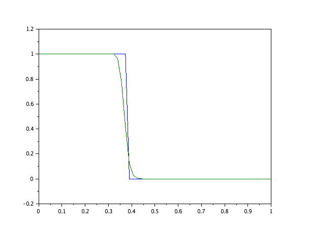
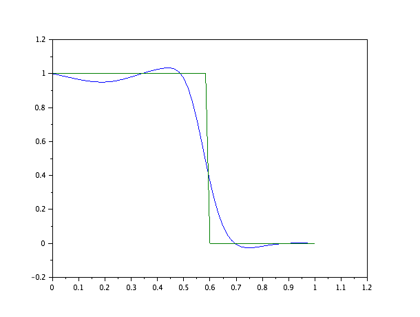
Figure 1: left Picard’s iteration with STILS-MT1 with penalization $\lambda=\frac{5}{12},$ right Picard’s iteration with simple finite element method

The mesh size of the space is $\frac{1}{60}$ and the times steep $\frac{1}{65}$ which give $60\times 65$ element in space-time. The solution is presented at $t=\frac{1}{4}$ in figure $1.$

Exemple 5.2

Let we choose now $\mu=7$ and compute the solution of by simple finite element method and STILS-MT1 with penalization $\lambda=\frac{5}{12}$ and using Newton Raphson iteration for the semi linearity.

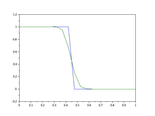
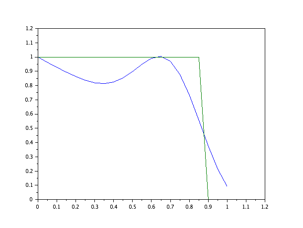
Figure 2: left Newton Adaptatif Raphson’s iteration with STILS-MT1 with penalization $\lambda=\frac{5}{12}$,rigth Newton adaptaif Raphson’s iteration with simple finite element method

The mesh size of the space is $\frac{1}{20}$ and the times steep $\frac{1}{25}$ which give $20\times 25$ element in space-time. The solution is presented at $t=\frac{1}{4}.$

Both numerical methods can be used to tame the spurious oscillations produced by STILS-MT and classical finite element methods when advection problem is solved. In the case of simple finite element methods, we have spurious diffusion for this semi-linear conservation, on the other hand the same fact can be obtaining when penalization version is used but it can be controlled by the parameter $\lambda$. Moreover, STILS-MT can not be used for simple finite element and that gives an important time calculation. We can clearly see that STILS-MT with penalization provides an effective methods for solving semi linear conservation law numerically.

References

- [1] Azerad P., Besson O. Inégalité de Poincaré courbe pour le traitement variationnel de l’équation de transport, C. R. Acad. Sci. Math, Paris, 322, 1996, 721-727.
- [2] Besson. O, de Montmolling. G. Space-time integred least squares : a time marching, internat.J.num.Methods Fluids , 44, 2004, 525–543
- [3] Besson. O, Pousin. J. Solutions for Linear Conservation Laws with Velocity Fields in , Archive for Rational Mechanics and Analysis, 2, 2007, 159–175
- [4] L. C. Evans. Partial Differential Equations. Graduate Studies in Mathematics,19, AMS,1998.
- [5] K. Benmansour; E. Bretin ; L. Piffet and J. Pousin Discrete Maximum principle for a space-time least squares formulation of the transport equation with finite element., Discrete and Continuous Dynamical Systems, 29 ,2011, 1001–1030.
- [6] P.A Raviart ; J.M.Thomas Introduction a l’analyse numérique des équations aux dérivées partielles ,Masson ,1992
- [7] H.Brezis ; Analyse fonctionnelle, Théorie et Applications, Collection Sciences Sup, Dunod, 2005
- [8] Perrochet. P, P. Azerad. Space-time integrated least squares:Solving a pure advection equation with a pure diffusion operator, J.Comput, Phys. 117, 1995, 183–193
- [9] H. Nguyen, J. Reynen. A space-time integrated least squares finite element scheme for advection-diffusion equation, Comput.Meths .Appl.Mech. Engrg., 42, 1984, 331–342
- [10] P. Azerad. Analyse des équations de Navier-Stokes en bassin peu profond et de l’équations de transport, thèse, Universite de Neutchatal , 1996.
- [11] C. Johnson and , U . Navert. Analysis of some finite element methods for some advection-diffusion problem , Res.Rep . 80.01,Dept.of comput Sciences , Chalmers University of Technology and University of Goteborg, Goteborg , Sweden, 1980.
- [12] Leopoldo P. Franca , G. Hauke , A. Masud . Revisiting finite elements methods for the advective-diffusive equation , Comput. Meths. Appl. Mech .Engrg., 195, 2006, 1560–1572.
- [13] D.N. Arnold, D. Boffi , R.S. Falk. Approximation by quadrilateral finite elements, Math. Comp. 71 239, 2002, 909–922.
- [14] J.L. Varona. Graphic and numerical comparison between iterative methods,Math. Intelligency, 24, 2002, 37–46.
- [15] H.R. Schneebeli and T.P. Wihler. The Newton-Raphson method and adaptive ODE solvers, Fractals. Complex,Geometry, Patterns, and Scaling in Nature and Society 19, 2011, 87–99.
- [16] M. Amrein and T.P. Wihler. An adaptive Newton-method based on a dynamical systems approach , Commun. Nonlinear Sci. Numer. Simul., 19, 2014, 2958–2973.
- [17] L. Mu, and X.Ye. A simple finite element methods for linear hyperbolic problem computational and Applied Mathematics, 2017
- [18] X.HU , L. Mu, and X.Ye. A simple finite element methods of the Cauchy problem for Poisson equation ,Numericals analysis and modelling 14, 2017,591–603.
- [19] B.Riviere Discontinuous Galerkin Methods for Solving Elliptic and Parabolic Equations: Theory and Implementation . SIAM 2008.
- [20] J. Wang and X. Ye, A weak A weak Galerkin mixed finite element method for second-order ellipticproblems, Math. Comp. 83, 2014, 2101–2126
- [21] H. RademacherUber partielle und totale differenzierbarkeit von Funktion mehrerer Variabeln und Uber die Transformation der Doppelintegrale, Mathematische Annalen. 79, 1919, 340–369
- [22] L. Ambrosio and P. Tilli Topics on analysis in metric spaces. Oxford University Press, Oxford, Oxford Lecture Series in Mathematics and its Applications 25 2004.
- [23] R.J. Leveque and H. C. Yee A stady of numerical methods for hyperbolic conservation laws with stiff source terms.Journal of Computational Physics 86, 1990 187-210.
- [24] H.O. Peitgen and P. H. Richter The beauty of fractals .Springer Verlag Berlin ,1986.