New Limits on Axionic Dark Matter from the Magnetar PSR J1745$-$2900

Abstract

Axions are a promising dark matter candidate that were motivated to solve the strong CP problem and that may also address the cosmological matter-antimatter asymmetry. Axion-photon conversion is possible in the presence of the strong magnetic fields, and the photon so produced will have energy equal to the axion mass. Here we report new limits on axionic dark matter obtained from radio spectra of the Galactic Center magnetar PSR J1745$-$2900. The magnetar has a magnetic field of $1.6\times 10^{14}$ G that interacts with a dark matter density $2\times 10^{5}$ to $2\times 10^{9}$ times greater than the local dark matter encountered by terrestrial haloscopes, depending on the Galactic dark matter profile. No significant spectral features are detected across 62% of the axion mass range 4.1–165.6 $\mu$eV (1–40 GHz). The interpretation of flux limits into limits on the two-photon coupling strength $g_{a\gamma\gamma}$ depends on the magnetospheric conversion model and on the dark matter density at the Galactic Center. For a standard dark matter profile, we exclude axion models with $g_{a\gamma\gamma}>$ 6–34 $\times 10^{-12}$ GeV^-1 with 95% confidence over the mass ranges 4.2–8.4, 8.9–10.0, 12.3–16.4, 18.6–26.9, 33.0–62.1, 70.1–74.3, 78.1–80.7, 105.5–109.6, 111.6–115.2, 126.0–159.3, and 162.5–165.6 $\mu$eV. For the maximal dark matter cusp allowed by stellar orbits near Sgr A*, these limits reduce to $g_{a\gamma\gamma}>$ 6–34 $\times 10^{-14}$ GeV^-1, which exclude some theoretical models for masses $>33$ $\mu$eV. Limits may be improved by modeling stimulated axion conversion, by ray-tracing conversion pathways in the magnetar magnetosphere, and by obtaining deeper broad-band observations of the magnetar.

1 Introduction

The Peccei-Quinn mechanism offers a solution to the strong $CP$ (charge-parity) problem in quantum chromodynamics (QCD) with the introduction of the axion, a spin zero chargeless massive particle (Peccei & Quinn, 1977; Weinberg, 1978; Wilczek, 1978). Moreover, QCD axions are a promising cold dark matter candidate (Preskill et al., 1983; Dine & Fischler, 1983; Abbott & Sikivie, 1983), and may explain the matter-antimatter asymmetry in the early universe (Co & Harigaya, 2019).

If axions ($a$) exist, they would have a two-photon coupling $g_{a\gamma\gamma}$ such that the electromagnetic interaction is

$$\mathcal{L}_{a\gamma\gamma}=-(1/4)g_{a\gamma\gamma}a\,F_{\mu\nu}\tilde{F}^{\mu\nu}=g_{a\gamma\gamma}a\,{\mathbf{E}}\cdot{\mathbf{B}}.$$ (1)

Axion-photon conversion can thus occur in the presence of a magnetic field, but the axion-photon coupling is weak: $g_{a\gamma\gamma}\sim 10^{-16}$ GeV^-1 for axion mass $m_{a}=1$ $\mu$eV (Kim, 1979; Shifman et al., 1980; Dine et al., 1981; Zhitnitskij, 1980; Sikivie, 1983). Theory predicts $g_{a\gamma\gamma}\propto m_{a}$, but the mass is not constrained. Axion searches must therefore span decades in $m_{a}$ while reaching very small $g_{a\gamma\gamma}$.

Axion experiments include CAST, which searched for Solar axions (Arik & et al., 2014, 2015), and “haloscopes” that use narrow-band resonant cavities to detect dark matter axions, such as ADMX and HAYSTAC (Asztalos & et al., 2001, 2010; Brubaker & et al., 2017; Zhong et al., 2018). There are also natural settings where one may use telescopes to conduct sensitive and wide-band QCD axion searches toward pulsars or galaxies (Hook et al., 2018; Huang et al., 2018; Day & McDonald, 2019; Leroy et al., 2020; Battye et al., 2020; Edwards et al., 2020; Mukherjee et al., 2020).

Of particular interest is the natural axion-photon conversion engine, the Galactic Center magnetar PSR J1745$-$2900. PSR J1745$-$2900 has a strong magnetic field ($1.6\times 10^{14}$ G; Mori & et al., 2013), and it should encounter the highest dark matter flux in the Galaxy (Hook et al., 2018). Axions will encounter a plasma frequency at some radius in the magnetosphere that equals its mass, allowing the axion to resonantly convert into a photon (Hook et al., 2018). The likely axion mass range, 1–100 $\mu$eV, equates to radio frequencies 240 MHz to 24 GHz.

In this Letter, we present archival observations of PSR J1745$-$2900 from the NSF’s Karl G. Jansky Very Large Array (VLA) that expand upon our previous work (Darling, 2020). We obtain 95% confidence limits on resonant axion-photon conversion emission line flux density from the magnetar spanning 62% of the 1–40 GHz band. Limits on the axion-photon coupling, $g_{a\gamma\gamma}$, rely on a neutron star magnetosphere model and are bracketed by two limiting-case uncored Galactic dark matter profiles. We present model caveats, discuss observational limitations, and suggest observational and theoretical work to expand the $g_{a\gamma\gamma}$ vs. $m_{a}$ space probed by this technique.

Table 1: Very Large Array Summary of Observations

Band	Frequency	Program	Channel Width		Median	$t_{\rm int}$	Median Beam	PA	MJD	rms
			Obs.	Sm.	Velocity
	(GHz)		(MHz)	(MHz)	(km s-1)	(s)	(arcsec)	(∘)		(mJy)
L	1.008–2.032	14A-231	1	10	2000	10591	$2.2\times 1.1$	1	56749	0.33
S	2.157–3.961	BP198	0.5	12	1172	26361	$3.1\times 1.2$	3	57577–57580	0.14
C	4.487–6.511	14A-231	2	14	763	10591	$0.61\times 0.28$	$-$3	56749	0.099
X	7.987–10.011	14A-231	2	18	600	19148	$0.34\times 0.17$	$-$1	56718	0.026
X	8.007–11.991	15A-418	2	18	539	27290	$0.68\times 0.38$	$-$53	57167–57173	0.098
Ku	12.038–13.060	12A-339	2	20	463	4086	$0.84\times 0.47$	3	56141–56143	0.066
Ku	12.988–15.012	14A-231	2	20	428	16156	$0.24\times 0.11$	$-$1	56726	0.027
Ku	16.951–17.961	12A-339	2	22	372	4086	$0.64\times 0.36$	$-$3	56141–56143	0.082
K	18.875–19.511	12A-339	2	22	349	8499	$0.58\times 0.28$	1	56065–56143	0.092
K	25.501–26.511	12A-339	2	24	285	8499	$0.43\times 0.20$	1	56065–56143	0.085
Ka	26.975–27.863	12A-339	2	26	275	8499	$0.37\times 0.17$	1	56065–56143	0.17
Ka	30.476–32.524	14A-232	2	26	247	17053	$0.101\times 0.050$	$-$3	56725	0.100
Ka	32.476–34.524	14A-232	2	26	233	17053	$0.094\times 0.046$	$-$3	56725	0.116
Ka	34.476–36.524	14A-232	2	28	236	17053	$0.089\times 0.045$	$-$4	56725	0.165
Ka	36.476–38.524	14A-232	2	28	224	17053	$0.084\times 0.042$	$-$3	56725	0.152
Ka	37.493–38.500	12A-339	2	28	221	8499	$0.28\times 0.13$	1	56065–56143	0.10
Q	39.300–40.052	12A-339	2	28	215	4413	$0.37\times 0.27$	36	56065–56123	0.22

Note. — Results for programs 14A-231 and 14A-232 were published in Darling (2020) and are reproduced here for completeness.

2 Observations

Darling (2020) used archival VLA observations of Sgr A* and/or PSR J1745$-$2900 (both are present in every primary beam), that have the highest angular resolution (A-array) in order to separate the magnetar from Sgr A* and to resolve out extended spectral line-emitting Galactic Center gas and extended continuum emission. The work presented here adds observations that are sub-optimal (B- and C-array) but which still enable the angular separation of Sgr A* from PSR J1745$-$2900. Unlike for the observations presented in Darling (2020), the PSR J1745$-$2900 radio continuum cannot be separated from the surrounding emission in these lower angular resolution data. Based on our previous confirmation of the astrometry of PSR J1745$-$2900 conducted by Bower et al. (2015), we are confident in our ability to extract a spectrum of PSR J1745$-$2900 from interferometric image cubes.

VLA observations of Sgr A* and PSR J1745$-$2900 were selected (1) to maximize on-target integration time, (2) with adequate angular resolution to separate PSR J1745$-$2900 from Sgr A* (1.7” in both coordinates), (3) to maximize total bandwidth, and (4) to adequately sample the expected emission line bandwidth. In addition to the VLA A-configuration programs 14A-231 and 14A-232 presented in Darling (2020), programs 12A-339, BP198, and 15A-418 meet these criteria and are analyzed in this Letter (Table 1).

Observing sessions used J1331+3030 (3C286) and J0137+331 (3C48) for flux calibration, 3C286, 3C48, and J1733$-$1304 for bandpass calibration, and J1744$-$3116, J1745$-$283, and J1751$-$2524 for complex gain calibration. Right- and left-circular polarizations were combined to form Stokes-I spectral cubes. Bandwidths of spectral windows were either 32 MHz or 128 MHz, subdivided into 0.5 or 2 MHz channels, respectively, and grouped into 2–4 overlapping basebands. All programs used 8-bit sampling except for 15A-418, which used 3-bit sampling. Correlator dump times were 1–5 s.

3 Data Reduction

We used CASA for interferometric data reduction. Data were flagged and calibrated (flux, delay, atmospheric transmission, complex bandpass, and complex gain). After applying calibration to the target field, we did in-beam phase self-calibration on the Sgr A* continuum (0.8–1.7 Jy from S- to Q-band).

We imaged the continuum in the target field and fit a 2D Gaussian to Sgr A* to set the origin for relative astrometry. We locate PSR J1745$-$2900 using the bootstrap proper motion solution obtained by Bower et al. (2015). Offsets were consistent between epochs in each band and between bands and were consistent with the observed continuum position of the magnetar detected in programs 14A-231 and 14A-232 (Darling, 2020).

After linear continuum subtraction in uv space, we formed spectral image cubes and cleaned these down to five times the theoretical noise. Sgr A* shows narrow-band spectral structure after the continuum subtraction, particularly in X-band where we see a comb of radio recombination lines (RRLs) in emission, but also due to spectral window edge effects. The RRLs are presumably mildly stimulated. We also see extended RRL emission in many spectral cubes due to the low angular resolution, and we see RRL emission toward the magnetar in some bands (see below). Sgr A* sidelobes are cleaned during cube deconvolution and do not significantly contaminate the magnetar spectrum, and the magnetar spectra typically reach the theoretical noise. Synthesized beams vary across each spectral cube due to the natural frequency-dependent angular resolution of the interferometer and due to data flagging and RFI.

We extract the magnetar spectrum over the 2D Gaussian beam and correct for the beam size for each channel in order to capture the total point source flux density. The spectral noise varies channel-to-channel, which can create false peaks in the magnetar spectrum. To assess significance of spectral features, we form a noise spectrum using a measurement of the sky rms noise in each channel. The overall noise spectrum is scaled to the spectral noise of PSR J1745$-$2900, which typically differ by a few percent.

For single-channel detection, we need to smooth spectra to the expected axion-photon conversion line width, but there is theoretical disagreement about the expected bandwidth of the emission line. Hook et al. (2018) make a conservation of energy argument to derive a fractional bandwidth that depends quadratically on the axion velocity dispersion $v_{0}$: $\Delta f/f=(v_{0}/c)^{2}$ (contrary to the intuitive expectation for the line width to reflect the velocity dispersion as a Doppler shift; Huang et al., 2018). Battye et al. (2020), however, suggest that the line width is dominated by the neutron star’s spinning magnetosphere. We adopt this spinning mirror model which produces, on average, a bandwidth $\Delta f/f\simeq\Omega\,r_{c}/c$, where $\Omega$ is the rotation angular frequency and $r_{c}$ is the axion-photon conversion radius. Hook et al. (2018) show that $r_{c}$ depends on the neutron star’s radius $r_{0}$, magnetic field $B_{0}$, angular frequency, polar orientation angle $\theta$, and magnetic axis offset angle $\theta_{m}$:

$$r_{c}=224~{}{\rm km}\times\left|3\cos\theta\ \hat{m}\cdot\hat{r}-\cos\theta_{m}\right|^{1/3}\times$$

$$~{}\left(r_{0}\over 10~{}{\rm km}\right)\left[{B_{0}\over 10^{14}~{}{\rm G}}{1\over 2\pi}{\Omega\over 1~{}{\rm Hz}}\left(4.1~{}\mu{\rm eV}\over m_{a}c^{2}\right)^{2}\right]^{1/3}$$ (2)

where $\hat{m}\cdot\hat{r}=\cos\theta_{m}\cos\theta+\sin\theta_{m}\sin\theta\cos\Omega t$. For now, we assume that $\theta=\pi/2$ and $\theta_{m}=0$ (we deal appropriately with these angles in Section 5) to obtain the expected line width:

$$\Delta f=3.6~{}{\rm MHz}\left(\Omega\over 1~{}{\rm Hz}\right)^{4/3}\left(m_{a}c^{2}\over 4.1~{}\mu{\rm eV}\right)^{1/3}\left(B_{0}\over 10^{14}~{}{\rm G}\right)^{1/3}$$ (3)

(4.1 $\mu$eV corresponds to 1 GHz as observed). PSR J1745$-$2900 has a 3.76 s rotation period (Kennea & et al., 2013) and a magnetic field of $1.6\times 10^{14}$ G (Mori & et al., 2013). The expected axion-photon conversion line width is thus $\Delta f=8.3~{}{\rm MHz}\times(m_{a}c^{2}/4.1~{}\mu{\rm eV})^{1/3}$. This corresponds to 2500 km s^-1 at 1 GHz and 215 km s^-1 at 40 GHz, which is generally broader than the expected dark matter dispersion, $\sim$300 km s^-1, except at the highest observed frequencies.

Spectra have flagged channels due to RFI and due to spectral window edges that lack the signal-to-noise for calibration. Flagged channels are much narrower than the expected line width, so we interpolate across these channels when smoothing using a Gaussian kernel (Price-Whelan et al., 2018). In some bands, such as L, S, and K, entire spectral windows can be flagged and all information is lost.

RRL emission lines are seen toward the magnetar in X-band (15A-418), Ku 12–13 GHz, Ku 17–18 GHz, and K 26 GHz. To remove RRLs, two 2 MHz channels are flagged per line, and subsequent smoothing interpolates across the flagged channels (the expected axion conversion line width is 18 MHz in X-band and 24 MHz at 26 GHz).

We combine spectra obtained from multiple observing sessions using an error-weighted average, and the sky (noise) spectra are combined in quadrature. When different observing programs overlap in frequency, we select the lowest-noise observation. This is effectively the same as combining overlapping spectra in quadrature because the less sensitive spectra contribute negligibly to an error-weighted mean.

Table 1 lists synthesized beam parameters, channel widths, and spectral rms noise values. Appendix A presents the new magnetar flux, noise, and signal-to-noise spectra.

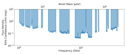
Figure 1: 95% confidence limits on axion-photon conversion line flux density. We present both linear (top) and logarithmic (bottom) scales for ease of comparison to other work.

4 Results

After smoothing to the expected axion-photon conversion line width, the new spectra show no significant ($>3\sigma$) single-channel emission features (Appendix A). The exception is a 3.2$\sigma$ channel at 2.34 GHz (9.67 $\mu$eV) in an RFI-affected region of S-band (there also two channels at 3.1$\sigma$ and 3.5$\sigma$ in previous Ka-band spectra; Darling, 2020).

We obtain single-channel 95% confidence limit flux density spectra from the sky noise spectra. Figure 1 shows the combined limits from this work and Darling (2020). These limits do depend on the assumed line width (Equation 3), which depends on the magnetar model, but these limits may be scaled as needed for magnetar models not treated in this Letter.

5 Analysis

Translating spectral flux density limits into limits on the axion-photon coupling $g_{a\gamma\gamma}$ depends on the axion-photon conversion in the magnetar magnetosphere and on the density of dark matter in the Galactic Center. Both of these rely on as-yet incompletely constrained models.

5.1 The Magnetar Model

We adopt the Hook et al. (2018) axion-photon conversion model for the magnetar magnetosphere, which is based on a variant of the Goldreich & Julian (1969) model (but note that there is substantial disagreement about the signal bandwidth and radiated power in the literature; e.g., Hook et al. (2018); Huang et al. (2018); Leroy et al. (2020); Battye et al. (2020)). We modify this model for the bandwidth adopted above (Equation 3) to obtain an expression for the observed flux density in the axion-photon conversion emission line that depends on the magnetar properties, distance, viewing angle $\theta$, and local dark matter density (see Darling, 2020, Equation 3).

Darling (2020) shows that given a flux density limit spectrum, one can produce a limit on $g_{a\gamma\gamma}$ as a function of $m_{a}$ that depends on the dark matter velocity dispersion $v_{0}$, the dark matter density $\rho_{\infty}$, and a time-dependent angular term involving $\theta$, $\theta_{m}$, and the axion velocity at the conversion point, $v_{c}^{2}\simeq 2GM_{NS}/r_{c}$ (Battye et al., 2020). For PSR J1745$-$2900 specifically, assuming a magnetar radius of 10 km, mass of 1 M_⊙, and distance of 8.2 kpc, we obtain

$$g_{a\gamma\gamma}=3\times 10^{-11}\ {\rm GeV}^{-1}\ \left(S_{\nu}\over 10\ \mu{\rm Jy}\right)^{1/2}\ \left(m_{a}\over 1\ {\rm GHz}\right)^{-2/3}\left(v_{0}\over 200\ {\rm km~{}s}^{-1}\right)^{1/2}\$$

$$\times\left(\rho_{\infty}\over 6.5\times 10^{4}\ {\rm GeV~{}cm}^{-3}\right)^{-1/2}\ \left({3(\hat{m}\cdot\hat{r})^{2}+1\over|3\cos\theta\ \hat{m}\cdot\hat{r}-\cos\theta_{m}|^{4/3}}{v_{c}\over c}\right)^{-1/2}.$$ (4)

The angular term relies on the unknown viewing and magnetic field misalignment angles and is time-dependent. Axion-photon conversion also relies on the conversion radius being outside the magnetar surface ($r_{c}>r_{0}$; see Equation 3), which is axion mass-dependent. For a given $(\theta,\theta_{m})$ pair, there may be parts of the magnetar rotation period that do not radiate. Since the modulation time is much less than the integration time of the observations, we average the expected signal over the period of the magnetar separately for each frequency channel for each $(\theta,\theta_{m})$ pair, to form time-integrated flux density spectra. We then marginalize over all $(\theta,\theta_{m})$ to obtain a limit spectrum on $g_{a\gamma\gamma}$ given a dark matter density and velocity dispersion (see below).

The ray-tracing performed by Leroy et al. (2020) suggests that this analytic treatment is conservative and that axion-photon conversion can occur over a larger parameter space. Nonetheless, the signal losses caused by angles where $r_{c}$ is always less than $r_{0}$ in this analytic treatment are a small fraction of the parameter space: at 10 GHz, 0.08% of all possible $(\theta,\theta_{m})$ always have $r_{c}<r_{0}$. This grows with frequency, and at 40 GHz the fraction of orientations with no emission rises to 6.6%.

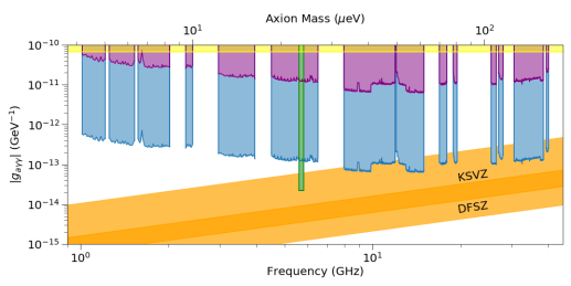
Figure 2: 95% confidence limits on $|g_{a\gamma\gamma}|$ for the NFW model prediction of the Galactic Center dark matter energy density (purple, upper) and the same NFW model plus a maximal central 100 pc dark matter spike (blue, lower). The HAYSTAC limit (green Zhong et al., 2018) has been scaled from a local axion density of 0.45 GeV cm^-3 to 0.38 GeV cm^-3. The yellow bar shows the CAST 95% confidence limit obtained from a search for solar axions (Anastassopoulos et al., 2017). The orange bands indicate the range of possible QCD axion models (Di Luzio et al., 2017), which include the canonical KSVZ and DFSZ models (Kim, 1979; Shifman et al., 1980; Dine et al., 1981; Zhitnitskij, 1980).

Table 2: Limits on the Axion-Photon Coupling $g_{a\gamma\gamma}$

Axion Mass	Median $|g_{a\gamma\gamma}|$ 95% Confidence Limits
	NFW Profile	DM Spike
($\mu$eV)	(GeV-1)	(GeV-1)
4.2–8.4	$3.4\times 10^{-11}$	$3.4\times 10^{-13}$
8.9–10.0	$2.9\times 10^{-11}$	$2.9\times 10^{-13}$
12.3–16.4	$1.7\times 10^{-11}$	$1.7\times 10^{-13}$
18.6–26.9	$1.3\times 10^{-11}$	$1.3\times 10^{-13}$
33.0–41.3	$6.9\times 10^{-12}$	$7.0\times 10^{-14}$
41.3–49.6	$1.1\times 10^{-11}$	$1.1\times 10^{-13}$
49.8–53.8	$1.0\times 10^{-11}$	$1.0\times 10^{-13}$
53.8–62.1	$6.5\times 10^{-12}$	$6.5\times 10^{-14}$
70.1–74.3	$1.0\times 10^{-11}$	$1.0\times 10^{-13}$
78.1–80.7	$1.1\times 10^{-11}$	$1.2\times 10^{-13}$
105.5–109.6	$1.0\times 10^{-11}$	$1.0\times 10^{-13}$
111.6–115.2	$1.5\times 10^{-11}$	$1.5\times 10^{-13}$
126.0–155.1	$1.4\times 10^{-11}$	$1.4\times 10^{-13}$
155.1–159.3	$1.3\times 10^{-11}$	$1.3\times 10^{-13}$
162.5–165.6	$2.2\times 10^{-11}$	$2.2\times 10^{-13}$

5.2 Dark Matter Models

The remaining unknowns in Equation 5.1 are the dark matter density $\rho_{\infty}$ and velocity dispersion $v_{0}$ at the location of the magnetar. The dark matter contribution in the Galactic Center has not been measured, so one must employ model-based interpolation. Following Hook et al. (2018), we adopt two models that roughly bracket the possible dark matter density (unless the dark matter distribution is cored; a multi-kpc central core is disfavored by observations (e.g. Hooper, 2017), and there are reasons to believe that baryon contraction has occurred (Cautun et al., 2020), but the existence of a cusp or core in the inner kpc remains observationally untested): a Navarro-Frenk-White (NFW; Navarro et al., 1996) dark matter profile and the same model plus a maximal dark matter cusp. For both models, we assume $v_{0}=300$ km s^-1 and a 0.1 pc separation between PSR J1745$-$2900 and Sgr A* (we identify Sgr A* with the center of the dark matter distribution). The 0.1 pc separation between PSR J1745$-$2900 and Sgr A* is projected, but absent an acceleration measurement one cannot know their true physical separation (Bower et al., 2015).

For the NFW dark matter profile, we adopt the McMillan (2017) fit with scale index $\gamma=1$, scale radius $r_{s}=18.6$ kpc, local dark matter energy density $\rho_{\odot}=0.38$ GeV cm^-3, and Galactic Center distance $R_{0}=8.2$ kpc, which agrees with the measurement by Abuter et al. (2019) of the orbit of the star S2 about Sgr A*. This model predicts a dark matter energy density of $6.5\times 10^{4}$ GeV cm^-3 at 0.1 pc.

The dark matter cusp model adds a spike to the NFW model with scale $R_{sp}=100$ pc and scale index $\gamma_{sp}=7/3$. This is the maximal dark matter spike corresponding to a 99.7% upper limit derived from a lack of deviations of the S2 star from a black hole-only orbit about Sgr A* (Lacroix, 2018). The maximal dark matter energy density encountered by the magnetar is thus $6.4\times 10^{8}$ GeV cm^-3, a factor of $10^{4}$ larger than the NFW-only model. This enhanced dark matter density corresponds to a 100-fold smaller constraint on $g_{a\gamma\gamma}$.

We present band-median 95% confidence limits on $|g_{a\gamma\gamma}|$ for each dark matter model in Table 2. Figure 2 shows the limit spectra spanning 62% of the 1–40 GHz (4.2–165.6 $\mu$eV) range, previous limits from CAST and HAYSTAC (Anastassopoulos et al., 2017; Zhong et al., 2018), and the family of theoretical axion models (Di Luzio et al., 2017). Limits obtained from the NFW model exclude $|g_{a\gamma\gamma}|\gtrsim$ 6–34 $\times 10^{-12}$ GeV^-1, which is 1.5–3.5 dex above the strongest-coupling theoretical prediction. The maximal dark matter spike model limits do, however, exclude portions of theoretical parameter space for $m_{a}=33.0$–165.6 $\mu$eV. The canonical KSVZ or DFSZ models are not excluded (Kim, 1979; Shifman et al., 1980; Dine et al., 1981; Zhitnitskij, 1980).

6 Discussion

The limits on $g_{a\gamma\gamma}$ presented here for the NFW profile are conservative compared to the Hook et al. (2018) predictions. This is due to the choice of a spinning-mirror bandwidth that seems more physically plausible (Battye et al., 2020). This bandwidth is $\mathcal{O}(v_{0}/c)$, roughly $10^{3}$ times larger than the Hook et al. (2018) $\mathcal{O}(v_{0}/c)^{2}$ bandwidth. This is a factor of $\sim$300 in $g_{a\gamma\gamma}$. A better treatment of this issue will require axion-photon conversion ray tracing as proposed by Leroy et al. (2020).

Our limits may also be conservative because resonant axion-photon conversion may be stimulated by the local photon occupation number, which would boost any signal thereby improving constraints on $g_{a\gamma\gamma}$ (Caputo et al., 2019). It seems likely that stimulated emission would be particularly important in the Galactic Center photon bath, but it may also arise naturally from the magnetar itself. This effect and numerical ray-tracing may significantly improve the constraints on $g_{a\gamma\gamma}$ based on the current observations alone.

As Figure 2 shows, the highly uncertain dark matter energy density in the inner parsec allows a large range of possible constraints on axion parameter space. Moreover, if the central dark matter is cored with a fixed NFW density of 12 GeV cm^-3 inward of 500 pc , then the limits on $g_{a\gamma\gamma}$ are degraded by 2 dex and lie above the CAST limits. We look forward to observational measurements of or constraints on the Galactic Center dark matter encountered by PSR J1745$-$2900 based on stellar and gas dynamics.

7 Conclusions

We have expanded the axion mass range searched for the axion-photon conversion signal originating from the magnetosphere of the Galactic Center magnetar PSR J1745$-$2900. New limits span 62% of the 4.2–165.6 $\mu$eV (1–40 GHz) axion mass range, excluding at 95% confidence $g_{a\gamma\gamma}>$ 6–34 $\times 10^{-12}$ GeV^-1 if the dark matter energy density follows a generic NFW profile at the Galactic Center. For a maximal dark matter spike, the limit reduces to $g_{a\gamma\gamma}>$ 6–34 $\times 10^{-14}$ GeV^-1, which excludes some possible axion models for $m_{a}>33$ $\mu$eV.

This work gets close to exhausting the appropriate data in the VLA archive. Lower resolution interferometric observations cannot separate the magnetar from the Sgr A* continuum, and we demonstrate how the extended Galactic Center continuum and line emission impairs the identification of the magnetar continuum and impacts the low angular resolution spectrum (particularly the RRL emission). Future observations designed to fill in the axion mass coverage or to increase sensitivity should use sub-arcsec resolution arrays. But high-resolution observations will exclude any axion-photon conversion signal that may arise from an extended population of Galactic Center neutron stars (Safdi et al., 2019).

It is unclear whether an axion-photon conversion signal will be pulsed. Analytic models suggest that it should be (e.g. Hook et al., 2018), but detailed ray-tracing and magnetosphere simulation are needed (Leroy et al., 2020). If emission is pulsed, future observations could in principle increase signal-to-noise by observing spectra in a gated pulsar mode.

Appendix A Spectra of the Magnetar PSR J1745$-$2900

Here we present the new radio spectra of the individual bands used to derive limits on the axion-photon coupling $g_{a\gamma\gamma}$ versus axion mass $m_{a}$ presented in the main Letter. Figures 3–11 show the flux density spectra, noise spectra, and significance spectra used for flux density and $g_{a\gamma\gamma}$ limits (Figures 1 and 2). Spectra obtained from VLA programs 14A-231 and 14A-232 (L-, C-, X-, Ku-, and Ka-bands listed in Table 1) are presented in Darling (2020).

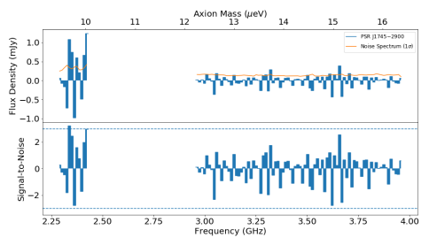
Figure 3: S-band flux density, noise, and signal-to-noise spectra. The upper spectrum can provide limits on $g_{a\gamma\gamma}$, while the lower spectrum shows the significance of spectral features.

Figure 4: X-band flux density, noise, and signal-to-noise spectra from VLA program 15A-418.

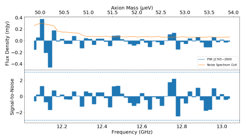
Figure 5: Ku-band 12–13 GHz flux density, noise, and signal-to-noise spectra.

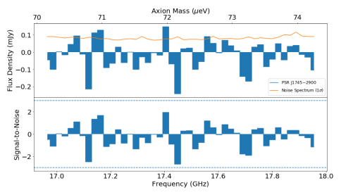
Figure 6: Ku-band 17–18 GHz flux density, noise, and signal-to-noise spectra.

Figure 7: K-band 18.9–19.5 GHz flux density, noise, and signal-to-noise spectra.

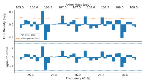
Figure 8: K-band 25.5–26.5 GHz flux density, noise, and signal-to-noise spectra.

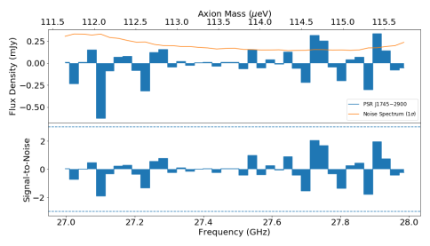
Figure 9: Ka-band 27–28 GHz flux density, noise, and signal-to-noise spectra.

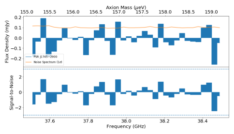
Figure 10: Ka-band 37.5–38.5 GHz flux density, noise, and signal-to-noise spectra.

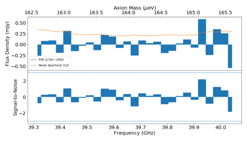
Figure 11: Q-band 39.3–40 GHz flux density, noise, and signal-to-noise spectra.

References

- Abbott & Sikivie (1983) Abbott, L. F., & Sikivie, P. 1983, Physics Letters B, 120, 133
- Abuter et al. (2019) Abuter, R., Amorim, A., Bauböck, M., et al. 2019, Astronomy & Astrophysics, 625, L10
- Anastassopoulos et al. (2017) Anastassopoulos, V., Aune, S., Barth, K., et al. 2017, Nature Physics, 13, 584
- Arik & et al. (2014) Arik, M., & et al. 2014, Phys. Rev. Lett., 112, 091302
- Arik & et al. (2015) —. 2015, Phys. Rev. D, 92, 021101
- Astropy Collaboration et al. (2013) Astropy Collaboration, Robitaille, T. P., Tollerud, E. J., et al. 2013, A&A, 558, A33
- Asztalos & et al. (2001) Asztalos, S. J., & et al. 2001, Phys. Rev. D, 64, 092003
- Asztalos & et al. (2010) —. 2010, Phys. Rev. Lett., 104, 041301
- Battye et al. (2020) Battye, R. A., Garbrecht, B., McDonald, J. I., Pace, F., & Srinivasan, S. 2020, Phys. Rev. D, 102, 023504
- Bower et al. (2015) Bower, G. C., Deller, A., Demorest, P., et al. 2015, The Astrophysical Journal, 798, 120
- Brubaker & et al. (2017) Brubaker, B. M., & et al. 2017, Phys. Rev. Lett., 118, 061302
- Caputo et al. (2019) Caputo, A., Regis, M., Taoso, M., & Witte, S. J. 2019, Journal of Cosmology and Astroparticle Physics, 2019, arXiv:1811.08436
- Cautun et al. (2020) Cautun, M., Benítez-Llambay, A., Deason, A. J., et al. 2020, MNRAS, 494, 4291
- Co & Harigaya (2019) Co, R. T., & Harigaya, K. 2019, arXiv e-prints, arXiv:1910.02080
- Darling (2020) Darling, J. 2020, Phys. Rev. Lett., in press, arXiv:2008.01877
- Day & McDonald (2019) Day, F. V., & McDonald, J. I. 2019, JCAP, 2019, 051
- Di Luzio et al. (2017) Di Luzio, L., Mescia, F., & Nardi, E. 2017, Physical Review Letters, 118, arXiv:1610.07593
- Dine & Fischler (1983) Dine, M., & Fischler, W. 1983, Physics Letters B, 120, 137
- Dine et al. (1981) Dine, M., Fischler, W., & Srednicki, M. 1981, Physics Letters B, 104, 199
- Edwards et al. (2020) Edwards, T. D. P., Chianese, M., Kavanagh, B. J., Nissanke, S. M., & Weniger, C. 2020, Phys. Rev. Lett., 124, 161101
- Goldreich & Julian (1969) Goldreich, P., & Julian, W. H. 1969, ApJ, 157, 869
- Hook et al. (2018) Hook, A., Kahn, Y., Safdi, B., & Sun, Z. 2018, Phys. Rev. Lett., 121, 241102
- Hooper (2017) Hooper, D. 2017, Physics of the Dark Universe, 15, 53
- Huang et al. (2018) Huang, F. P., Kadota, K., Sekiguchi, T., & Tashiro, H. 2018, Physical Review D, 97, 123001
- Hunter (2007) Hunter, J. D. 2007, Computing in Science Engineering, 9, 90
- Kennea & et al. (2013) Kennea, J. A., & et al. 2013, ApJ, 770, L24
- Kim (1979) Kim, J. E. 1979, Phys. Rev. Lett., 43, 103
- Lacroix (2018) Lacroix, T. 2018, Astronomy and Astrophysics, 619, 46
- Leroy et al. (2020) Leroy, M., Chianese, M., Edwards, T. D. P., & Weniger, C. 2020, Phys. Rev. D, 101, 123003
- McMillan (2017) McMillan, P. J. 2017, MNRAS, 465, 76
- McMullin et al. (2007) McMullin, J. P., Waters, B., Schiebel, D., Young, W., & Golap, K. 2007, 127
- Mori & et al. (2013) Mori, K., & et al. 2013, ApJ, 770, L23
- Mukherjee et al. (2020) Mukherjee, S., Spergel, D. N., Khatri, R., & Wand elt, B. D. 2020, JCAP, 2020, 032
- Navarro et al. (1996) Navarro, J. F., Frenk, C. S., & White, S. D. M. 1996, ApJ, 462, 563
- Peccei & Quinn (1977) Peccei, R. D., & Quinn, H. R. 1977, Phys. Rev. Lett., 38, 1440
- Preskill et al. (1983) Preskill, J., Wise, M. B., & Wilczek, F. 1983, Phys. Lett. B, 120, 127
- Price-Whelan et al. (2018) Price-Whelan, A. M., Sipőcz, B. M., Günther, H. M., et al. 2018, AJ, 156, 123
- Safdi et al. (2019) Safdi, B. R., Sun, Z., & Chen, A. Y. 2019, Physical Review D, 99, arXiv:1811.01020
- Shifman et al. (1980) Shifman, M. A., Vainshtein, A. I., & Zakharov, V. I. 1980, Nuclear Physics B, 166, 493
- Sikivie (1983) Sikivie, P. 1983, Phys. Rev. Lett., 51, 1415
- van der Walt et al. (2011) van der Walt, S., Colbert, S. C., & Varoquaux, G. 2011, Computing in Science Engineering, 13, 22
- Weinberg (1978) Weinberg, S. 1978, Phys. Rev. Lett., 40, 223
- Wilczek (1978) Wilczek, F. 1978, Phys. Rev. Lett., 40, 279
- Zhitnitskij (1980) Zhitnitskij, A. R. 1980, Yadernaya Fizika, 31, 497
- Zhong et al. (2018) Zhong, L., Al Kenany, S., Backes, K. M., et al. 2018, Physical Review D, 97, 092001