Improving Deep Stereo Network Generalization with Geometric Priors
Abstract
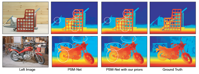
End-to-end deep learning methods have advanced stereo vision in recent years and obtained excellent results when the training and test data are similar. However, large datasets of diverse real-world scenes with dense ground truth are difficult to obtain and currently not publicly available to the research community. As a result, many algorithms rely on small real-world datasets of similar scenes or synthetic datasets, but end-to-end algorithms trained on such datasets often generalize poorly to different images that arise in real-world applications. As a step towards addressing this problem, we propose to incorporate prior knowledge of scene geometry into an end-to-end stereo network to help networks generalize better. For a given network, we explicitly add a gradient-domain smoothness prior and occlusion reasoning into the network training, while the architecture remains unchanged during inference. Experimentally, we show consistent improvements if we train on synthetic datasets and test on the Middlebury (real images) dataset. Noticeably, we improve PSM-Net accuracy on Middlebury from 5.37 MAE to 3.21 MAE without sacrificing speed.
1 Introduction
Capturing scene geometry or depth is a basic task for computer vision. Despite the development of high-quality 3D sensors, there are still numerous drawbacks such as added hardware and cost. Stereo vision provides an excellent alternative where depth is estimated using two images captured simultaneously from two vantage points. Stereo estimation is a classical computer vision problem that has been intensively studied due to its wide applications.
Recent supervised deep neural networks have significantly improved the performance in stereo depth estimation. But these networks are data hungry, and it is difficult to obtain large and diverse real-world stereo depth datasets with dense and accurate ground truth. Existing datasets, e.g., [7, 14, 15, 16], rely on LiDAR or structured light to obtain the ground truth. However, it is challenging to synchronize LiDAR with the stereo cameras, especially with moving objects. For example, creators of the KITTI stereo benchmark dataset [7, 14] manually fit 3D models to cars to obtain depth ground-truth of moving pixels, and mask out bicyclists and pedestrians. Deep models trained with such datasets work well on test images of the same dataset but typically do not generalize well to other datasets. Since it is difficult to obtain a real-world dataset for diverse scene types, there is a necessity for the design of robust deep neural networks that can generalize well from training on synthetic data.
In this work, we propose techniques to improve generalization across datasets. We do this with novel training modules that incorporate scene geometry priors into the network training. Specifically, we propose two different training modules. The first module encourages piecewise smoothness in estimated depths. This is based on the common knowledge that scenes are usually composed of a number of continuous surfaces, and thus the depth varies piecewise smoothly across image pixels. The second module explicitly models the relationship between occlusions and disparities given by the rectified camera geometry. Together, these modules help the network capture geometric scene information that is invariant across different datasets. Since both network modules are back-propagatable, they can be used to augment any stereo network during training to improve the updating of the network parameters. During inference, however, only the original network is used, thus ensuring that neither runtime nor parameters are increased for any given network.
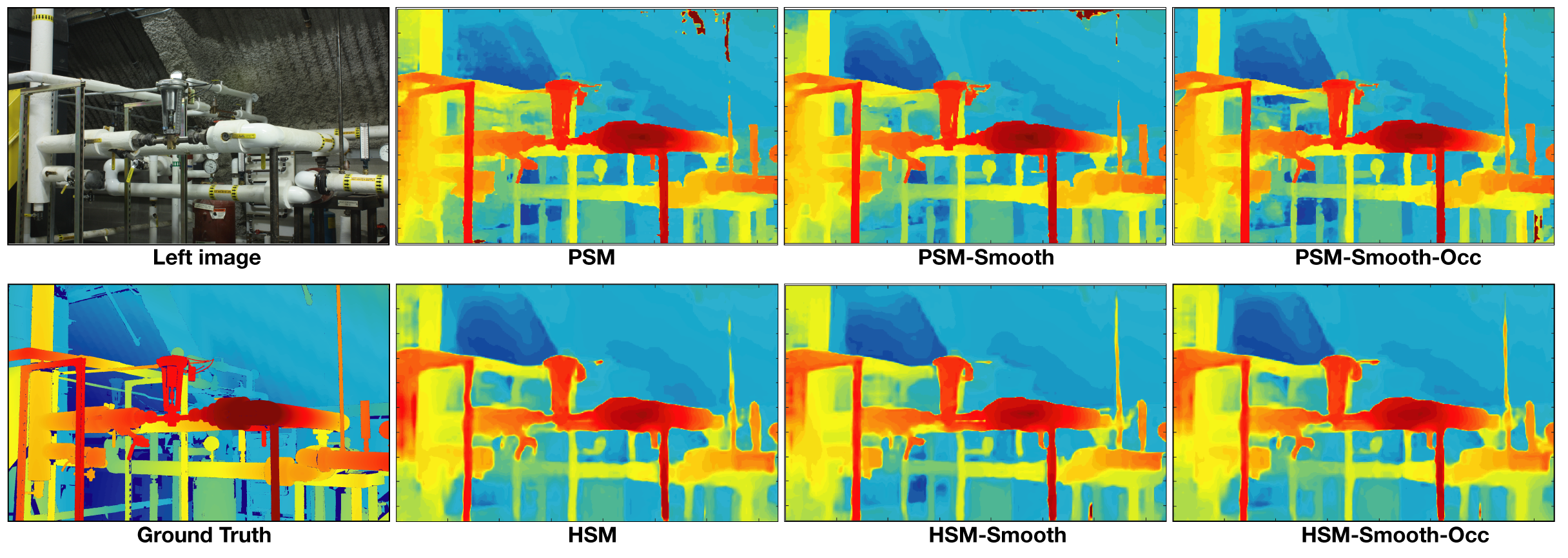
We empirically analyze the use of the proposed modules on two recent deep stereo networks: PSM-Net [5] and HSM-Net [27]. Experiments using synthetic training datasets (FlyingThings3D [13] and Falling Things [21]) and real testing datasets (Middlebury [15]) show consistent improvements due to our training modules. Figure 1 shows sample results indicating less noise in textureless regions and more fine details.
2 Related Work
Since a comprehensive stereo review is out of scope, we discuss the most relevant papers.
Traditional approaches. Classical methods typically first build a cost volume by comparing local patches at different disparity using image pixel intensity values or hand-crafted features (e.g. census transform [29]). The cost volume is then processed by a global optimization method, such as semi-global matching [9] or graph cut [12] to get a regularized disparity map. Finally, some post-processing steps are usually adopted to improve the disparity map.
Deep-learning approaches. Zbontar and LeCun [30] propose using Siamese networks to learn matching features to replace hand-crafted ones, and achieve better stereo results. Mayer et al. [13] propose an end-to-end CNN stereo algorithm, which computes correlation between CNN features to construct a 1D cost volume and process it using CNN layers. Kendall et al. [10] propose concatenating features to construct the cost volume and processing it using 3D convolutions, which is GPU-memory-intensive and relatively slow.
Chang and Chen introduce the PSM-Net [5], which uses spatial pyramid pooling modules and stacked-hourglass modules to improve the accuracy. However, PSM-Net still uses 3D convolutions and cannot process high-resolution images because of GPU memory constraints. Later methods reduce the computational overhead and/or aim for high-resolution images [11, 27, 22, 24, 20, 28]. In particular, HSM-Net [27] estimates disparity in a coarse-to-fine manner, and uses novel data augmentation methods to achieve state-of-the-art in mean absolute error (MAE) in the high-resolution Middlebury dataset while running with low latency. In this paper, we test our proposed priors on both PSM-Net and HSM-Net and show concrete improvements over the two strong baseline methods.
Post-processing. Barron and Poole [6] propose using a fast bilateral solver on the disparity map predicted by the MC-CNN [30] and achieve a lower MAE. Cheng et al. [6] add a convolutional spatial propagation network module on top of a deep stereo architecture inspired by the PSM-Net. However, these works introduce additional computation at test time. In contrast, we add the proposed geometric priors during the training time to improve the parameters of the baseline networks without adding additional computation at test time.
Prior constraints for stereo. There are several notable works on improving stereo with prior constraints, e.g. [31, 26]. Most noticeably, Woodford et al. [26] use visibility test and second-order smoothness priors in a classical stereo algorithm. They detect occlusions by the mapping uniqueness criterion [4, 25]. Our work revisits the second-order smoothness prior in an end-to-end trainable framework. We determine occlusion maps from disparity maps directly using the projective geometry (explained in Section 3.2) and add a loss term that incorporates a gradient-domain prior to train a deep stereo network.
3 Preliminaries
In this section, we describe preliminaries of the two key components of our method: 1) pixel-adaptive convolutions, and 2) the relationship between disparities and occlusions for a rectified stereo image pair.
3.1 Pixel-adaptive convolutions
We make use of recently proposed pixel-adaptive convolutions (PAC) [17] to incorporate learned smoothness priors on estimated disparities. Here, we briefly review PAC and will describe the use of PACs in our framework in Section 4.1. Following the notation from [17], standard convolution of image features with input channels and output channels; with filter can be written as
| (1) |
where are pixel coordinates, denotes a 2D slice of the 4D tensor , defines an neighborhood, and denotes biases. One of the core properties of standard spatial convolution is spatial-invariance as the filter only depends on position offsets . PAC provides a generalization of standard convolution in CNNs by adapting filter at each pixel with a content-adaptive kernel that depends on pixel features :
| (2) |
where is a kernel function that has a fixed parametric form such as Gaussian: , where are guidance features. PAC generalizes other widely used filtering operations such as bilateral filtering [1, 19].
3.2 Relationship between disparities and occlusions
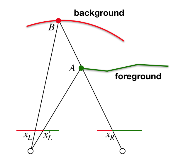
Given any disparity map , we can directly estimate an occlusion map in a principled way using rectified camera geometry [2, 23]. Here we review the mathematical relationship using the left image as the reference image. Figure 2(a) shows an example of a foreground surface and a background surface. Assuming rectified geometry and both principal points located at the image center, by the definition of disparity we have at the occlusion boundary point on the foreground, and at the first mutually visible pixel on the background. Subtracting both sides yields . Therefore, the number of occluded pixels is equal to the disparity difference.
4 Method
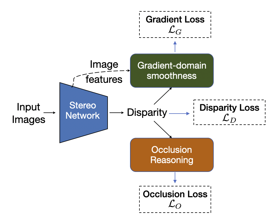
We propose adding two priors into the training of an existing deep network as additional supervision. Figure 2(b) shows the overview of our architecture.
4.1 Gradient-domain smoothness prior
A typical stereo loss function minimizes some loss metric on disparity (e.g., loss). This loss treats all regions on the image equally, and it sometimes fails to model desirable properties of the disparity. Using the insight that many surfaces in the scene are approximately planar, we enforce a gradient-domain smoothness prior by processing the disparity gradient and with a gradient smoothness module consisting of PAC layers to filter the gradient to yield a refined gradient and . Intuitively, PAC layers output similar values for two nearby pixels when the guidance features ( in Eqn. 2) at those pixels are similar, while preserving the discontinuity at places where the features change dramatically (e.g., object boundaries). Note that, unlike applying a PAC module directly to the disparity map itself, which would tend to assign the same disparity values to surfaces with similar features, applying a PAC module to and (as we do) naturally models slanted planes and allows quadratic surfaces. Prior researchers have also found that second-order priors in the gradient domain can better model the world [26, 3, 8, 18]. Although the guidance features for the PAC module could simply be the RGBXY values of the image [17], additional information is captured by the image features that are already learned in early stages of the network. Experimentally we have found that, in many cases, the learned features achieve better performance.
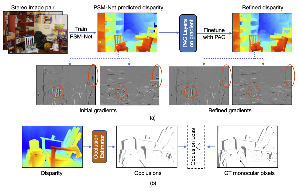
Figure 3(a) shows an example of the effect of PAC layers on disparity gradients. The baseline PSM-Net [5] (top row) trained with only disparity loss produces noisy disparity gradients in background slanted planes and near foreground object boundaries, whereas after finetuning with PAC-refined gradients loss, the noise is significantly reduced.

4.2 Occlusion reasoning
We can deterministically estimate an occlusion map using the equations described in Section 3.2 without adding additional parameters into the baseline network. To compute a “soft” occlusion map at a pixel for back propagation, we use a “steep” Sigmoid function to approximate a step function:
| (3) |
where and . The parameter controls the slope. The offset is needed because is always positive, leading to a skewed distribution. We conducted a grid search to find the optimal parameters, and we found and gave us good occlusion estimates. Figure 3(b) shows an example of our estimated left occlusion map (middle) from the ground truth disparity map (left), in comparison with the ground truth left monocular mask (right) provided by the Middlebury dataset.
4.3 Total loss function
We propose to finetune a state-of-the-art stereo network using the following loss function to improve the network’s weights.
| (4) |
where,
Here, is the disparity loss, is the gradient domain smoothness loss and is the occlusion loss. We use smooth loss for , and .
5 Experiments
As discussed above, designing robust deep neural networks that can generalize well from training on synthetic data is especially important for stereo because the ground truth for real images is hard to obtain, and sometimes has its own noise (e.g. the “ground truth” obtained using LiDAR). As a step towards this direction, we evaluate the proposed methods using three datasets: FlyingThings3D [13] and Falling Things [21] as training datasets, and Middlebury [15] as the test dataset.
We analyze our proposed modules with two state-of-the-art end-to-end trainable stereo networks discussed in Related Work, PSM-Net [5] and HSM-Net [27]. Our technique is agnostic to the base stereo network architecture. That is, we only add additional parameters and computations during training. So, our inference runtime is exactly the same as the baseline. For brevity, we will refer to our occlusion reasoning module as “Occ” and our gradient-smoothness module via PAC filtering as “GradSmooth”.
5.1 Datasets and Evaluation
FlyingThings3D [13] consists of a large number of synthetic images with 3D objects flying around in space. It is one of the three scenes in the SceneFlow [13] dataset. The FlyingThings3D test set is the same as the SceneFlow test set.
Falling Things [21] is a recent synthetic dataset of household objects with realistic rendering. We used the “mixed” sequences with more than one foreground object.
Middlebury 2014 [15] is a high-resolution real-image stereo dataset. Figures 1, 3, 5 and 6 show some dataset images. We test on all 23 Middlebury scenes that have ground truth, which include “evaluation training sets” and “additional training images”. We use their “perfect” images with balanced lighting. Since Middlebury images are of higher resolution than FlyingThings3D and Falling Things, we evaluate on quarter-resolution Middlebury images, similar to some other methods [9, 5].
Evaluation Metrics All the results we report in this section are on ALL pixels that have ground truth. We evaluate using two standard stereo metrics: bad-2.0 (the percentage of pixels in which , and MAE (the mean absolute error).
5.2 Implementation details
In all our experiments, we use two PAC layers sequentially in a GradSmooth module. The first PAC layer is a convolutional layer with a dilation of 4. The second PAC layer is a convolutional layer with a dilation of 8 and then output a filtered disparity gradient. With PSM-Net, we add one GradSmooth module for each resolution, thus in total three GradSmooth modules. In HSM-Net, we add one GradSmooth module at the highest resolution . We set in our loss function. In experiments without occlusion reasoning (denoted as PSM-GradSmooth or HSM-GradSmooth), we simply drop the occlusion term in the loss function. We use incremental training in our experiments, which means we first train a given base network, and then finetune it with our added modules.
5.3 Robustness with geometric priors
FlyingThings3D. One of the main metrics researchers use to compare different stereo networks is the test set accuracy on the same (but disjoint) dataset images used in training (e.g. SceneFlow). We observe that if we finetune PSM-Net (starting with the authors’ weights) with only FlyingThings3D data in the SceneFlow dataset, we can achieve state-of-the-art 0.63 MAE111Same as the original PSM-Net, we only evaluate on pixels with disparity due to GPU memory limit. for the SceneFlow test set. However, the network overfits to the synthetic data, as evidenced by the very high test error we observe on Middlebury (27.46 MAE). See Figure 4. This suggests that network robustness is a more important metric to optimize. Specifically, we define robustness as the network’s ability to generalize when trained on synthetic images and then tested on real images. As discussed before, it is highly desirable to design and train networks using synthetic images that can generalize well.
Table 1 shows the quantitative comparison. For PSM-Net, with the author’s published weights trained on SceneFlow [5], the test MAE on Middlebury is 16.91. After finetuning only on FlyingThings3D, the best model’s MAE is reduced to 5.37. After further finetuning with the GradSmooth module, the MAE is further reduced to 4.62, and with both GradSmooth and Occ modules, the error is reduced to 3.21. Again, this is all done without reducing speed at test time.
| Architecture | Train | Test | bad-2.0 | MAE |
| PSM (author weights) | SF | MB | 29.67 | 16.91 |
| PSM | FT3D | MB | 19.58 | 5.37 |
| PSM-GradSmooth | FT3D | MB | 19.04 | 4.62 |
| PSM-GradSmooth-Occ | FT3D | MB | 18.17 | 3.21 |
| HSM | FT3D | MB | 25.56 | 3.00 |
| HSM-GradSmooth | FT3D | MB | 22.09 | 2.71 |
| HSM-GradSmooth-Occ | FT3D | MB | 25.24 | 3.06 |
For HSM-Net [27], we observe that the GradSmooth module helps improve upon the baseline HSM-Net, but not the Occ module. One possible reason could be that the sophisticated occlusion augmentation that HSM-Net performs on the training images may have a complicated interaction with our occlusion module. Further, the ground truth disparity may be missing in some occluded regions on the Middlebury dataset, making it hard to evaluate the improvement brought by the occlusion reasoning module.
Figures 1 and 5 show some qualitative results. In general, networks trained with our geometric priors predict disparity maps with less noise in the smooth regions, and the boundaries align better with the actual object boundaries than those trained without the geometric priors.
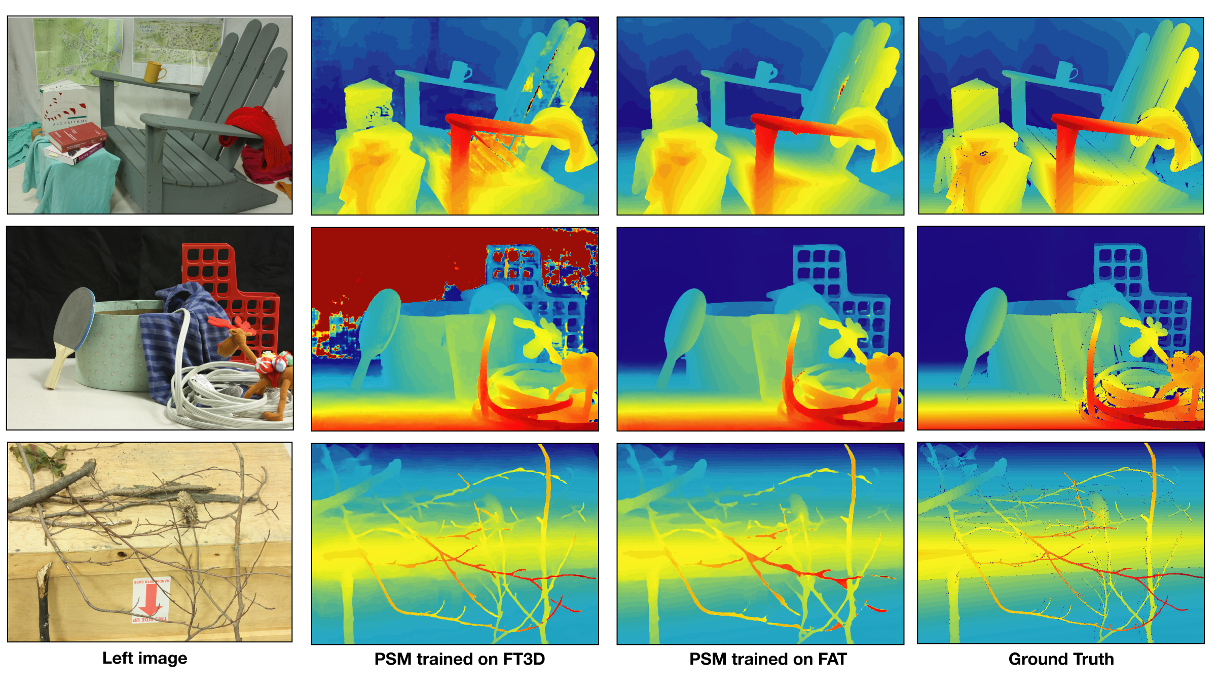
Falling Things. We also train PSM-Net with the newer Falling Things dataset [21] and compare the results with models trained with the more popular FlyingThings3D dataset. Table 2 shows that PSM-Net trained with Falling Things significantly outperforms the same network trained on FlyingThings3D [13]. Even with Falling Things, the GradSmooth module we propose still helps the performance, improving the percentage of bad pixels to 10.35.
Figure 6 shows the qualitative comparison between PSM-Net trained on FlyingThings3D and Falling Things. PSM-Net trained with FlyingThings3D often fails on textureless regions (rows 1-2). However, the predictions by models trained on Falling Things sometimes lack fine details (e.g. row 3).
| Architecture | Train | Test | bad-2.0 | MAE |
| PSM | FT3D | MB | 19.58 | 5.37 |
| PSM | FT3D | MB | 11.48 | 1.41 |
| PSM-GradSmooth | FT3D | MB | 10.35 | 1.42 |
6 Conclusion
As a step towards designing robust stereo networks, we propose adding two priors into the stereo networks based on our knowledge of scene geometry. Our proposed geometric priors neither add computation nor require extra memory at inference time. Extensive experiments show that adding a gradient-domain smoothness prior consistently improves generalization and, in some cases, adding occlusion prior further improves generalization.
References
- [1] Volker Aurich and Jörg Weule. Non-linear gaussian filters performing edge preserving diffusion. In Mustererkennung 1995. Springer, 1995.
- [2] Peter N Belhumeur. A Bayesian approach to binocular stereopsis. IJCV, 1996.
- [3] Andrew Blake and Andrew Zisserman. Visual reconstruction. 1987.
- [4] Myron Z Brown, Darius Burschka, and Gregory D Hager. Advances in computational stereo. IEEE TPAMI, 2003.
- [5] Jia-Ren Chang and Yong-Sheng Chen. Pyramid stereo matching network. In CVPR, 2018.
- [6] Xinjing Cheng, Peng Wang, and Ruigang Yang. Learning depth with convolutional spatial propagation network. arXiv:1810.02695, 2018.
- [7] Andreas Geiger, Philip Lenz, and Raquel Urtasun. Are we ready for autonomous driving? the KITTI vision benchmark suite. In CVPR, 2012.
- [8] William Eric Leifur Grimson. From images to surfaces: A computational study of the human early visual system. MIT press, 1981.
- [9] Heiko Hirschmuller. Stereo processing by semiglobal matching and mutual information. IEEE TPAMI, 2007.
- [10] Alex Kendall, Hayk Martirosyan, Saumitro Dasgupta, Peter Henry, Ryan Kennedy, Abraham Bachrach, and Adam Bry. End-to-end learning of geometry and context for deep stereo regression. In ICCV, 2017.
- [11] Sameh Khamis, Sean Fanello, Christoph Rhemann, Adarsh Kowdle, Julien Valentin, and Shahram Izadi. StereoNet: Guided hierarchical refinement for real-time edge-aware depth prediction. In ECCV, 2018.
- [12] Vladimir Kolmogorov and Ramin Zabih. Computing visual correspondence with occlusions via graph cuts. Technical report, 2001.
- [13] Nikolaus Mayer, Eddy Ilg, Philip Hausser, Philipp Fischer, Daniel Cremers, Alexey Dosovitskiy, and Thomas Brox. A large dataset to train convolutional networks for disparity, optical flow, and scene flow estimation. In CVPR, 2016.
- [14] Moritz Menze and Andreas Geiger. Object scene flow for autonomous vehicles. In CVPR, 2015.
- [15] Daniel Scharstein, Heiko Hirschmüller, York Kitajima, Greg Krathwohl, Nera Nešić, Xi Wang, and Porter Westling. High-resolution stereo datasets with subpixel-accurate ground truth. In German conference on pattern recognition, 2014.
- [16] Thomas Schöps, Johannes L. Schönberger, Silvano Galliani, Torsten Sattler, Konrad Schindler, Marc Pollefeys, and Andreas Geiger. A multi-view stereo benchmark with high-resolution images and multi-camera videos. In CVPR, 2017.
- [17] Hang Su, Varun Jampani, Deqing Sun, Orazio Gallo, Erik Learned-Miller, and Jan Kautz. Pixel-adaptive convolutional neural networks. In CVPR, 2019.
- [18] Demetri Terzopoulos. Multilevel computational processes for visual surface reconstruction. Computer Vision, Graphics, and Image Processing, 1983.
- [19] Carlo Tomasi and Roberto Manduchi. Bilateral filtering for gray and color images. In ICCV, 1998.
- [20] Alessio Tonioni, Fabio Tosi, Matteo Poggi, Stefano Mattoccia, and Luigi Di Stefano. Real-time self-adaptive deep stereo. In CVPR, 2019.
- [21] Jonathan Tremblay, Thang To, and Stan Birchfield. Falling things: A synthetic dataset for 3D object detection and pose estimation. In CVPR Workshops, 2018.
- [22] Stepan Tulyakov, Anton Ivanov, and Francois Fleuret. Practical deep stereo (PDS): Toward applications-friendly deep stereo matching. In NeurIPS, 2018.
- [23] Jialiang Wang and Todd Zickler. Local detection of stereo occlusion boundaries. In CVPR, 2019.
- [24] Yan Wang, Zihang Lai, Gao Huang, Brian H Wang, Laurens van der Maaten, Mark Campbell, and Kilian Q Weinberger. Anytime stereo image depth estimation on mobile devices. In ICRA, 2019.
- [25] Yichen Wei and Long Quan. Asymmetrical occlusion handling using graph cut for multi-view stereo. In CVPR, 2005.
- [26] Oliver Woodford, Philip Torr, Ian Reid, and Andrew Fitzgibbon. Global stereo reconstruction under second-order smoothness priors. IEEE TPAMI, 2009.
- [27] Gengshan Yang, Joshua Manela, Michael Happold, and Deva Ramanan. Hierarchical deep stereo matching on high-resolution images. In CVPR, 2019.
- [28] Kyle Yee and Ayan Chakrabarti. Fast deep stereo with 2D convolutional processing of cost signatures. arXiv:1903.04939, 2019.
- [29] Ramin Zabih and John Woodfill. Non-parametric local transforms for computing visual correspondence. In ECCV, 1994.
- [30] Jure Zbontar, Yann LeCun, et al. Stereo matching by training a convolutional neural network to compare image patches. Journal of Machine Learning Research, 2016.
- [31] Chi Zhang, Zhiwei Li, Rui Cai, Hongyang Chao, and Yong Rui. As-rigid-as-possible stereo under second order smoothness priors. In ECCV, 2014.