The atomic damping basis and the collective decay of interacting two-level atoms

Abstract

We find analytical solutions to the evolution of interacting two-level atoms when the master equation is symmetric under the permutation of atomic labels. The master equation includes atomic independent dissipation. The method to obtain the solutions is: First, we use the system symmetries to describe the evolution in an operator space whose dimension grows polynomially with the number of atoms. Second, we expand the solutions in a basis composed of eigenvectors of the dissipative part of the master equation that models the independent dissipation of the atoms. This atomic damping basis is an atomic analog to the damping basis used for bosonic fields [1]. The solutions show that the system decays as a sum of sub- and super-radiant exponential terms.

Keywords: Quantum optics, Collective effects in quantum optics, Superradiance and subradiance.

1 Introduction

Emission processes by interacting quantum emitters exhibit collective effects [2, 3, 4, 5]. An example of a quantum emitter is an atom. Atoms can interact with one another through electromagnetic fields. In free space, collective effects appear when the distance between the atoms is of the order of the wavelength associated with the atomic transition [6, 7, 8, 9]. When the quantum emitters consist of an array of two-level atoms near 1D nanowaveguides, the atomic interaction is mediated by guided modes. In this case, the atoms can be far apart and interact with each other, showing collective effects [10, 11, 12, 13, 14].

Sub- and super- radiance are signatures of collective effects. As an example, consider two-level atoms in free space. An atom initially in the excited state will decay exponentially with a rate $\Gamma$. Something similar happens with several two-level atoms with atomic distances much larger than the wavelength associated with the atomic transition. Independently of the initial state, an excitation of a given atom decays exponentially with rate $\Gamma$, that is, with the same rate as one atom. If the atoms are close enough, of the order of the wavelength associated with the atomic transition, the interaction with each other through the electromagnetic field cannot be neglected. We focus on the regime where all the atoms are close enough that if a photon is emitted by an atom, the probability to be reabsorbed by another is negligible. In this case, the decay of $N$ excited atoms depends strongly on the initial state [6, 7, 8, 9]. For example, if the initial state has one excitation, but this excitation is shared by all atoms through a superposition, the atoms decay exponentially. But the decay rate can be faster or slower than $\Gamma$ depending on the superposition phases. When interacting atoms decay faster than independent atoms, we say that the system decay is super-radiant. If the decay is slower we say it is sub-radiant. In order to have a modification of the decay rate, coherence between the different quantum emitters is necessary. Coherence can be generated externally, for example driving the atoms with a laser. Also, it can appear without using an external source. In states with more than one excitation without initial coherence, coherence appears as the number of excited atoms diminishes with time. Coherence creation is a consequence of atomic interaction through the electromagnetic field [15].

The exponential growth of the number of degrees of freedom with the number of interacting atoms is one obstacle to studying theoretically these systems. Analytic solutions for the collective decay have been found for two [16, 17] and three atoms [8]. To reduce the exponential complexity for several atoms one can use the symmetries on the system or study the thermodynamic limit ($N\to\infty$) [18, 19]. Also, there are methods that truncate the Hilbert space of the system, as in the Matrix Product State Method [20], or constraining the number of total excitations [9].

If both the master equation, that describes the state evolution, and the initial condition have symmetries, the evolution of $N$ atoms takes place in a subspace of operators with a reduced number of degrees of freedom. An example of this is the super-radiance master equation without atomic independent decay, where the symmetric Dicke basis can be used to find solutions [21]. When atomic independent decay is included in the super-radiance equation, the symmetric Dicke basis is no longer useful, and one has to use numerical methods to solve the system for a large number of atoms [15]. Nevertheless, the super-radiance equation with independent atomic decay can be (depending on the position of the atoms) symmetric under permutation in atomic labels. In this case, the space of operators acting on the symmetric subspace of the Hilbert space grows polynomially with the number of atoms. This symmetric subspace of two-level atoms has been described by Xu et al. [22] using symmetry transformations of SU(4). Efficient numerical simulations can be performed using the symmetric subspace [23, 24, 25]. The use of the permutation symmetry has been generalized to $n$-level systems. Thus, the multiplets of SU($n^{2}$) have been proposed as a basis (called basis of symmetric operators) for the symmetric subspace. In addition, the generators of SU($n^{2}$) (also called collective superoperators) are used to express any linear map [26] on the symmetric subspace.

To get analytical expressions for the evolution of a quantum state, besides using symmetries to reduce the size of the system space, it is helpful to find a basis where the evolution of the state takes a simple form. In the case of master equations that describe electromagnetic fields in the presence of dissipation (quantum optical master equations), damping bases [1] have been useful to obtain analytical solutions. In this approach, the solution is expanded in a basis given by the eigenvectors of the non-Hermitian part of the master equation. The method has proven to be helpful in describing the process of laser cooling [27, 28], optomechanical systems [29] and the engineering of quantum states [30].

The purpose of this paper is to describe the evolution of $N$ interacting two-level atoms using analytical solutions that we obtain when the master equation is symmetric under the permutation of atomic indexes. We focus on the case in which the master equation, in the interaction picture, has only dissipative (independent and collective) terms (section 2). An example of this kind of systems is a unidimensional equidistant array of atoms near a nanofiber. For this system, we use the basis of symmetric operators (section 3) to find the eigenvectors of the non-Hermitian part of the master equation describing atomic independent spontaneous decay (section 4). These eigenvectors form a basis, the atomic damping basis, that generalizes for a symmetric system of $N$ atoms the idea of a basis for the atomic damping of one two-level atom [1]. The atomic damping basis codifies in a convenient way the independent decay of the atoms. Expanding the solution in this basis we find analytical expressions using perturbation theory, when the interaction between the atoms is weak (section 5), and solving the differential equations for the coefficients in the expansion in the general case (section 6).

We focus on the evolution of a symmetric Dicke and a symmetric mixed state as initial conditions. The symmetric Dicke state exemplifies the case where the initial state has coherence between its components, whereas the symmetric mixed state exemplifies the case where there is no initial coherence between the components. The symmetric mixed state is particularly interesting since it shows collective behavior (super-radiance and sub-radiance), which implies that coherence between the components has been created as the system decays. In an experiment, comparing the decay dynamics exemplified by these two cases can be useful to detect if the initial state has coherence between its components. Analytical expressions are obtained when at most $M=4$ atoms are excited from a total of $N$.

There are two main results in this work: First, the atomic damping basis for the symmetric operator subspace that codifies the dissipation of $N$ independent atoms and, as shown in sections 5 and 6, is helpful to obtain solutions of master equations describing interacting atoms. Second, analytical expressions for the mean number of excited atoms showing the decay as a sum of sub- and super-radiant exponential terms. The weight of each exponential depends on the parameters of the system and the initial condition. The prediction of super- and sub-radiant decay in this problem is not new [15], but the analytical expressions we derive are helpful to understand and predict interesting behavior for different values of the system parameters. For example, consider the case where the interaction between atoms is strong and the initial condition consists of a mixed state where $3$ atoms, from a total of $N\gg 3$, are excited, but we do not know which ones. The evolution of this system creates coherence in such a way that the sub-radiant decay dominates the evolution at all times and, as the interactions between the atoms is strong, the decay rate is very slow.

2 System

We study $N$ two-level atoms interacting through the electromagnetic field without external drive. We denote by $|0\rangle^{(\mu)}$ the ground state and by $|1\rangle^{(\mu)}$ the excited state of atom $\mu$. We denote by $\mathcal{L}$ the Hilbert space of operators acting on the system Hilbert space. This space is known as the Liouville space [31]. An operator $O$ is denoted as $\hat{O}$, except when we refer to a state operator or an element of the damping basis where we use the rounded ket $\left|O\right)$.

A linear map $B$ acting on the elements of a Liouville space (also called superoperator) is denoted by $\breve{B}$. Thus, the operator state $\left|\tilde{\rho}\right)\in\mathcal{L}$ satisfies the master equation

$$\frac{d}{dt}\left|\tilde{\rho}\right)=-\frac{i}{\hbar}\left[\hat{H}_{0}+\hat{H}_{\textrm{int}},\left|\tilde{\rho}\right)\right]+\breve{L}\left|\tilde{\rho}\right)\,.$$ (1)

The unitary part of the evolution is given by the Hamiltonian of the atoms

$$\hat{H}_{0}=\frac{\hbar\omega_{0}}{2}\sum_{\mu=1}^{N}\hat{\sigma}_{z}^{(\mu)}\,,$$ (2)

where $\hat{\sigma}_{z}^{(\mu)}=|1\rangle^{(\mu)}{}^{(\mu)}\langle 1|-|0\rangle^{(\mu)}{}^{(\mu)}\langle 0|$, and the dipolar-dipolar interaction between atoms mediated by the field is [32]

$$\hat{H}_{\textrm{int}}=\hbar\sum_{\mu,\,\nu}\Omega_{\mu,\,\nu}\hat{\sigma}_{+}^{(\mu)}\hat{\sigma}_{-}^{(\nu)}\,,$$ (3)

where $\hat{\sigma}_{-}^{(\mu)}=|0\rangle^{(\mu)}{}^{(\mu)}\langle 1|=(\hat{\sigma}_{+}^{(\mu)})^{\dagger}$.

The non-unitary part of the evolution is described by $\breve{L}=\breve{L^{\prime}}_{i}+\breve{L^{\prime}}_{c}$. The first non-unitary term is the independent atomic decay modeled by

$$\breve{L^{\prime}}_{i}\bullet = \Gamma\sum_{\mu=1}^{N}\Big{(}\hat{\sigma}_{-}^{(\mu)}\bullet\hat{\sigma}_{+}^{(\mu)}-\frac{1}{2}\hat{\sigma}_{+}^{(\mu)}\hat{\sigma}_{-}^{(\mu)}\bullet-\frac{1}{2}\bullet\hat{\sigma}_{+}^{(\mu)}\hat{\sigma}_{-}^{(\mu)}\Big{)}\,,$$ (4)

and the second term is the collective dissipation [33]

$$\breve{L^{\prime}}_{c}\bullet = \sum_{\mu=1\,\nu=1,\mu\neq\nu}^{N}\gamma_{\mu\,\nu}\Big{(}\hat{\sigma}_{-}^{(\nu)}\bullet\hat{\sigma}_{+}^{(\mu)}-\frac{1}{2}\hat{\sigma}_{+}^{(\mu)}\hat{\sigma}_{-}^{(\nu)}\bullet-\frac{1}{2}\bullet\hat{\sigma}_{+}^{(\mu)}\hat{\sigma}_{-}^{(\nu)}\Big{)}\,.$$ (5)

Here $\Gamma$ is the independent atomic spontaneous emission rate and $\gamma_{\mu\,\nu}$ is proportional to the interaction between the atoms. When the atoms do not interact with each other, $\gamma_{\mu\,\nu}=0$, and $\Gamma$ gives the rate at which each atom decays. We will focus on the case where $\gamma_{\mu\,\nu}=\gamma_{c}\leq\Gamma$. In this case we can write $\breve{L}=\breve{L}_{i}+\breve{L}_{c}$ with

$$\breve{L}_{i}\bullet = (\Gamma-\gamma_{c})\sum_{\mu=1}^{N}\Big{(}\hat{\sigma}_{-}^{(\mu)}\bullet\hat{\sigma}_{+}^{(\mu)}-\frac{1}{2}\hat{\sigma}_{+}^{(\mu)}\hat{\sigma}_{-}^{(\mu)}\bullet-\frac{1}{2}\bullet\hat{\sigma}_{+}^{(\mu)}\hat{\sigma}_{-}^{(\mu)}\Big{)}\,,$$ (6)

and

$$\breve{L}_{c}\bullet = \gamma_{c}\bigg{[}\hat{J}_{-}\bullet\hat{J}_{+}-\frac{1}{2}\hat{J}_{+}\hat{J}_{-}\bullet-\frac{1}{2}\bullet\hat{J}_{+}\hat{J}_{-}\bigg{]}\,,$$ (7)

where the collective atomic operators are $\hat{J}_{\pm}=\sum_{\mu}\hat{\sigma}_{\pm}^{(\mu)}$. This equation is symmetric under interchange of atomic operator labels.

Examples where independent and collective dissipation terms, as the ones we are considering, appear are atoms near a nanowaveguide [32] or inside a leaky cavity [15]. In the case of a nanowaveguide (see figure 1), the guided electromagnetic modes introduce long distance interactions between the atoms. Assuming that the atoms are far apart (the distance between them is larger than the atomic transition wavelength) the not-guided (radiative) modes do not introduce dipolar-dipolar interaction terms. Thus, dipolar coupling between atoms is given only through the guided modes. This unitary contribution, given by the Hamiltonian (3), is a function of atomic position. If we denote by $z_{\mu}$ the position of atom $\mu$ along the fiber axial axis, $\Omega_{\mu,\,\nu}$ is proportional to the sine of $\beta\left(z_{\mu}-z_{\nu}\right)$ [11], with $\beta$ the propagation constant [10]. As we are interested only in the effect of dissipation terms, we consider interatomic distances such that $\Omega_{\mu,\,\nu}=0$, making (3) zero.

We simplify the master equation (1) using the interaction picture. We define

$$\left|\rho\right)=\hat{U}^{\dagger}\left|\tilde{\rho}\right)\hat{U}\,$$

with $\hat{U}=\exp{\left(-i\hat{H}_{0}t/\hbar\right)}$. Considering that $\hat{U}^{\dagger}\hat{\sigma}_{\pm}^{(\mu)}\hat{U}=\exp(\pm i\omega_{0}t)\hat{\sigma}_{\pm}^{(\mu)}$ and $\hat{H}_{\textrm{int}}=0$, Eq. (1) in the interaction picture reads

$$\frac{d}{dt}\left|\rho\right)=\breve{L}\left|\rho\right)\,.$$ (8)

Under these conditions we have two processes of spontaneous emission. First, we have independent dissipation where atoms emit photons into radiative modes; second, we have collective dissipation into the guided modes. Assuming that the atoms are located in positions with the same coupling to the nanowaveguide, the master equation for the system is (8) with $\breve{L}=\breve{L}_{i}+\breve{L}_{c}$.

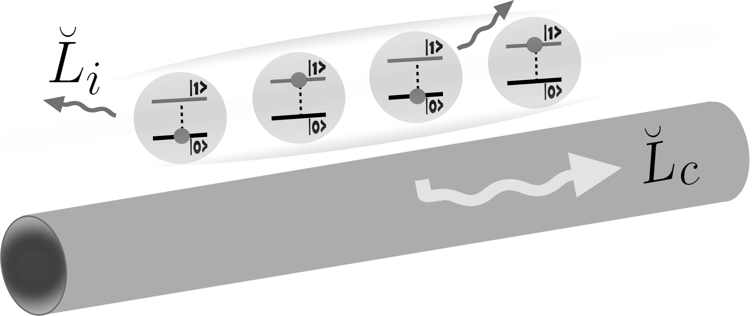
Figure 1: Representation of the two dissipation processes for two-level atoms in the vicinity of a nanofiber. In the independent dissipation, represented by $\breve{L}_{i}$, the atoms emit to free space. In the guided collective dissipation, $\breve{L}_{c}$, the atoms can interact between each other even if they are far apart and emit along the guided mode of the nanofiber.

The formal solution of Eq. (8) is $\left|\rho(t)\right)=e^{\breve{L}t}\left|\rho(0)\right)$, with $\left|\rho(0)\right)$ the initial condition. Our goal is to find $\left|\rho(t)\right)$ by writing the solution as a superposition of the right eigenvectors of $\breve{L}_{i}$, which satisfy

$$\breve{L}_{i}\left|\alpha\right)=\lambda_{\alpha}\,\left|\alpha\right)\,,$$ (9)

where $\lambda_{\alpha}$ is a complex number. Due to the fact that $\breve{L}_{i}$ is non-Hermitian, there is no guarantee that a basis of the Liouville space with the eigenvectors of this linear map exists. When the set $\{\left|\alpha\right):\breve{L}_{i}\left|\alpha\right)=\alpha\left|\alpha\right)\}$ forms a basis, it will be called the atomic damping basis. We denote the dual space of $\mathcal{L}$ as $\mathcal{L}^{*}$. Given $\left(\alpha\right|\in\mathcal{L}^{*}$ we define the inner product as

$$\left(\alpha^{\prime}\middle|\alpha\right)\equiv\Tr[\left(\alpha^{\prime}\right|^{\dagger}\left|\alpha\right)]\,.$$

We use the bra-type notation to indicate that $\left(\alpha\right|$ is the dual of $\left|\alpha\right)$. The elements of $\mathcal{L}^{*}$ are not necessarily the Hermitian conjugates of the elements of $\mathcal{L}$. Therefore, to expand a system state in the damping basis we need to compute the left eigenvectors

$$\left(\alpha\right|\breve{L}_{i}=\lambda_{\alpha}\,\left(\alpha\right|\,,$$ (10)

where $\left(\alpha\right|\in\mathcal{L}^{*}$ and satisfy the duality relation

$$\left(\alpha^{\prime}\middle|\alpha\right)=\delta_{\alpha^{\prime},\alpha}\,.$$ (11)

With a basis of right and left eigenvectors we can solve the equation of motion (8). For $\breve{L}_{c}=0$ we get

$$\left|\rho(t)\right)=\sum_{\alpha}e^{\lambda_{\alpha}t}c_{\alpha}\left|\alpha\right),$$ (12)

where we used the corresponding left eigenvectors and Eq. (11) to calculate $c_{\alpha}=\left(\alpha\middle|\rho(0)\right)$.

In general the solution will be of the form

$$\left|\rho(t)\right)=\sum_{\alpha}e^{\lambda_{\alpha}t}c_{\alpha}(t)\left|\alpha\right)\,,$$ (13)

where the coefficients $c_{\alpha}(t)$ are found using the master equation.

In the following sections we obtain the damping basis for the symmetric subspace of $N$ atoms and use it to obtain analytical expressions for the master equation (8) when $\breve{L}_{c}\neq 0$. The damping basis method has been used to obtain analytical solutions for bosonic systems [1]. The program we present here generalizes the idea of the damping basis for one two-level atom [1] to a symmetric system of $N$ atoms.

3 Symmetric subspace

The Hilbert space of $N$ two-level atoms is given by the tensor product $\mathcal{H}_{2}\otimes\mathcal{H}_{2}\otimes\cdots\otimes\mathcal{H}_{2}=\mathcal{H}_{2}^{\otimes N}$, where $\mathcal{H}_{2}$ is the space of one two-level atom. The Hilbert space of operators acting on $\mathcal{H}_{2}$, the one-atom Liouville space, is denoted by $\mathcal{L}_{4}$. For $N$ atoms the Liouville space is $\mathcal{L}_{4}^{\otimes N}$ and consists of all the operators that act on the elements of $\mathcal{H}_{2}^{\otimes N}$. This operator space has dimension $4^{N}$. This exponential growth is reduced when the system is symmetric under interchange of particle labels. Over the elements of $\mathcal{L}_{4}^{\otimes N}$ we can define the permutation of labels between any pair of particles $i$ and $j$. The operators invariant under any permutation form the symmetric subspace, denoted by $\mathcal{S}(\mathcal{L}_{4}^{\otimes N})$, with dimension $(N+1)(N+2)(N+3)/6$ [22, 34]. Because the Lindblad operators (6) and (7) remain the same under any permutation, the evolution of an initial state in $\mathcal{S}(\mathcal{L}_{4}^{\otimes N})$ under $\breve{L}$ is constrained to the symmetric subspace.

We introduce a basis for the space $\mathcal{S}(\mathcal{L}_{4}^{\otimes N})$ [34]. The elements of this basis, called basis of symmetric operators, are [26]

$$\hat{Q}^{\mbox{\scriptsize$\begin{array}[]{cc}n_{00}&n_{01}\\ n_{10}&n_{11}\end{array}$}} = \frac{n_{00}!n_{01}!n_{10}!n_{11}!}{N!}\sum_{P}\breve{P}\Big{(}\left|00\right)^{\otimes n_{00}}\left|01\right)^{\otimes n_{01}}\left|10\right)^{\otimes n_{10}}\left|11\right)^{\otimes n_{11}}\Big{)}\,,$$ (16)

where $\left|mn\right)=|m\rangle\langle n|$, $m,n=0,1$, is a basis of $\mathcal{L}_{4}$ [31]. For the tensor products in (16) we introduce exponents $n_{mn}=0,1,2,\ldots,N$, which satisfy the constraint $N=n_{00}+n_{01}+n_{10}+n_{11}$. With this, we denote the tensor product as $\left|mn\right)^{\otimes n_{mn}}=\otimes^{n_{mn}}_{k=1}\left|mn\right)$ for nonzero $n_{mn}$. We use $P$ to indicate some permutation of $\left|00\right)^{\otimes n_{00}}\left|01\right)^{\otimes n_{01}}\left|10\right)^{\otimes n_{10}}\left|11\right)^{\otimes n_{11}}$ and $\breve{P}$ to refer to the superoperator that gives the permutation. As an example, the symmetric mixed state of two atoms in the ground state and one atom excited is

$$\hat{Q}^{\mbox{\scriptsize$\begin{array}[]{cc}2&0\\ 0&1\end{array}$}}=\frac{1}{3}\bigg{(}\left|00\right)\left|00\right)\left|11\right)+\left|00\right)\left|11\right)\left|00\right)+\left|11\right)\left|00\right)\left|00\right)\bigg{)}\,,$$

where for simplicity we omit the notation of the tensor product. The symmetric operators are mutually orthogonal and satisfy

$$\Tr\left(\hat{Q^{\dagger}}^{\mbox{\scriptsize$\begin{array}[]{cc}n_{00}^{\prime}&n_{01}^{\prime}\\ n_{10}^{\prime}&n_{11}^{\prime}\end{array}$}}\hat{Q}^{\mbox{\scriptsize$\begin{array}[]{cc}n_{00}&n_{01}\\ n_{10}&n_{11}\end{array}$}}\right) = \frac{n_{00}!n_{01}!n_{10}!n_{11}!}{N!}\delta_{n_{00}^{\prime},n_{00}}\delta_{n_{01}^{\prime},n_{01}}\delta_{n_{10}^{\prime},n_{10}}\delta_{n_{11}^{\prime},n_{11}}\,.$$ (22)

Not all the symmetric operators represent physical states, but any operator state in $\mathcal{S}(\mathcal{L}_{4}^{\otimes N})$ can be represented by linear combinations of these operators.

We introduce the ladder-type superoperators $\breve{A}^{\mbox{\scriptsize$\begin{array}[]{cc}ij\\ kl\end{array}$}}_{+}$. These can be written as a sum of $N$ local terms $\big{(}\breve{A}^{\mbox{\scriptsize$\begin{array}[]{cc}ij\\ kl\end{array}$}}_{+}\big{)}^{(\mu)}$. On the Liouville space of each particle we define bosonic superoperators $\breve{b}_{mn}^{(\mu)},\,\breve{b}_{mn}^{{\dagger}(\mu)}$ for $m,\,n=0,\,1$. The superoperator $\breve{b}_{mn}^{(\mu)}$ annihilates the operator $\left|mn\right)^{(\mu)}$, while $\breve{b}_{mn}^{(\mu){\dagger}}$ creates the operator. With these bosonic superoperators we define $\big{(}\breve{A}^{\mbox{\scriptsize$\begin{array}[]{cc}ij\\ kl\end{array}$}}_{+}\big{)}^{(\mu)}=\breve{b}_{ij}^{(\mu){\dagger}}\breve{b}_{kl}^{(\mu)}$, thus the collective superoperators are equal to [26]

$$\breve{A}^{\mbox{\scriptsize$\begin{array}[]{cc}ij\\ kl\end{array}$}}_{+}=\sum_{\mu=1}^{N}\breve{b}_{ij}^{(\mu){\dagger}}\breve{b}_{kl}^{(\mu)}\,.$$ (25)

The superoperators $\breve{b}$ satisfy the usual rules of commutation $\big{[}\breve{b}_{ij}^{(\mu)},\breve{b}_{kl}^{(\mu){\dagger}}\big{]}=\delta_{ij,\,kl}$ and $\big{[}\breve{b}_{ij}^{(\mu)},\breve{b}_{kl}^{(\mu)}\big{]}=\big{[}\breve{b}_{ij}^{(\mu){\dagger}},\breve{b}_{kl}^{(\mu){\dagger}}\big{]}=0$. We introduce the bosonic superoperators only as an algebraic support to define the collective superoperators.

From (25) we have that $\breve{A}^{\mbox{\scriptsize$\begin{array}[]{cc}ij\\ kl\end{array}$}}_{+}$ acting on the left of $\hat{Q}^{\mbox{\scriptsize$\begin{array}[]{cc}n_{00}&n_{01}\\ n_{10}&n_{11}\end{array}$}}$ decrease the label $n_{kl}$ by one and increase $n_{ij}$ by one, and the resulting operator is multiplied by $n_{kl}$. For example

$$\breve{A}^{\mbox{\scriptsize$\begin{array}[]{cc}11\\ 10\end{array}$}}_{+}\hat{Q}^{\mbox{\scriptsize$\begin{array}[]{cc}n_{00}&n_{01}\\ n_{10}&n_{11}\end{array}$}} = n_{10}\hat{Q}^{\mbox{\scriptsize$\begin{array}[]{cc}n_{00}&n_{01}\\ n_{10}-1&n_{11}+1\end{array}$}}.$$ (32)

The action of $\breve{A}^{\mbox{\scriptsize$\begin{array}[]{cc}ij\\ kl\end{array}$}}_{+}$ to the right side of $\hat{Q^{\dagger}}^{\mbox{\scriptsize$\begin{array}[]{cc}n_{00}&n_{01}\\ n_{10}&n_{11}\end{array}$}}=\hat{Q}^{\mbox{\scriptsize$\begin{array}[]{cc}n_{00}&n_{10}\\ n_{01}&n_{11}\end{array}$}}$ is obtained by replacing $n_{kl}\leftrightarrow n_{ij}$ above. For example

$$\hat{Q^{\dagger}}^{\mbox{\scriptsize$\begin{array}[]{cc}n_{00}&n_{01}\\ n_{10}&n_{11}\end{array}$}}\breve{A}^{\mbox{\scriptsize$\begin{array}[]{cc}11\\ 10\end{array}$}}_{+} = n_{11}\hat{Q^{\dagger}}^{\mbox{\scriptsize$\begin{array}[]{cc}n_{00}&n_{01}\\ n_{10}+1&n_{11}-1\end{array}$}}.$$ (39)

4 Atomic damping basis

We write $\breve{L}_{i}$ in terms of collective superoperators to solve the eigenvalue problem (9) on the symmetric subspace,

$$\breve{L}_{i}\left|\rho\right) = \gamma_{10}\bigg{[}\breve{A}^{\mbox{\scriptsize$\begin{array}[]{cc}00\\ 11\end{array}$}}_{+}-\breve{A}^{\mbox{\scriptsize$\begin{array}[]{cc}11\\ 11\end{array}$}}_{+}-\frac{1}{2}\bigg{(}\breve{A}^{\mbox{\scriptsize$\begin{array}[]{cc}10\\ 10\end{array}$}}_{+}+\breve{A}^{\mbox{\scriptsize$\begin{array}[]{cc}01\\ 01\end{array}$}}_{+}\bigg{)}\bigg{]}\left|\rho\right)\,,$$ (48)

where $\gamma_{10}=\Gamma-\gamma_{c}$. In A we show some useful formulas to obtain the results presented here. As eigenvectors we propose linear combinations of symmetric operators as

$$\left|\rho_{sym}\right)=\sum_{n_{ij}}c^{\mbox{\scriptsize$\begin{array}[]{cc}n_{00}&n_{01}\\ n_{10}&n_{11}\end{array}$}}\hat{Q}^{\mbox{\scriptsize$\begin{array}[]{cc}n_{00}&n_{01}\\ n_{10}&n_{11}\end{array}$}}\,.$$ (53)

Using the action of the collective superoperators we find that

$$\breve{L}_{i}\hat{Q}^{\mbox{\scriptsize$\begin{array}[]{cc}n_{00}&n_{01}\\ n_{10}&n_{11}\end{array}$}} = \gamma_{10}\bigg{[}n_{11}\hat{Q}^{\mbox{\scriptsize$\begin{array}[]{cc}n_{00}+1&n_{01}\\ n_{10}&n_{11}-1\end{array}$}}-n_{11}\hat{Q}^{\mbox{\scriptsize$\begin{array}[]{cc}n_{00}&n_{01}\\ n_{10}&n_{11}\end{array}$}}-\frac{n_{10}+n_{01}}{2}\hat{Q}^{\mbox{\scriptsize$\begin{array}[]{cc}n_{00}&n_{01}\\ n_{10}&n_{11}\end{array}$}}\bigg{]}\,.$$

With the previous equation and substituting (53) into (48) we obtain the recurrence relation

$$c^{\mbox{\scriptsize$\begin{array}[]{cc}n_{00}-1&n_{01}\\ n_{10}&n_{11}+1\end{array}$}} = \frac{1}{n_{11}+1}\left(\frac{N}{2}+\frac{n_{11}-n_{00}}{2}+\frac{\lambda}{\gamma_{10}}\right)c^{\mbox{\scriptsize$\begin{array}[]{cc}n_{00}&n_{01}\\ n_{10}&n_{11}\end{array}$}}\,.$$ (59)

Solving the recurrence relation we obtain that the eigenvalues are

$$\lambda_{\alpha,\delta}=-\gamma_{10}\bigg{[}\frac{N-\alpha}{2}+\delta\bigg{]},$$ (60)

where $\alpha=n_{00}+n_{11}$ and $0\leq\delta\leq\alpha$ is an integer. The right eigenvectors are defined by

$$\left|\alpha,\delta\right)_{n}=(-1)^{\delta}\left(\begin{array}[]{c}N\\ \alpha\end{array}\right)\left(\begin{array}[]{c}N-\alpha\\ n\end{array}\right)\left(\begin{array}[]{c}\alpha\\ \delta\end{array}\right)\sum_{n_{11}=0}^{\delta}(-1)^{n_{11}}\left(\begin{array}[]{c}\delta\\ n_{11}\end{array}\right)\hat{Q}^{\mbox{\scriptsize$\begin{array}[]{cc}\alpha-n_{11}&N-\alpha-n\\ n&n_{11}\end{array}$}}\,.$$ (71)

For simplicity we denote $n=n_{10}$, which we use to identify the different degenerate eigenvectors. The eigenvector with $\alpha=N$ and $\delta=0$, $\left|N,0\right)_{0}$, represents the ground state. The other eigenvectors do not represent physical states because their trace is zero. We use them because they are algebraically easy to manipulate, any symmetrical physical state can be represented by a superposition of $\left|\alpha,\delta\right)_{n}$, and allow us to obtain analytical solutions.

The right eigenvectors (71) are linearly independent. They are also degenerate because the label $n$ can take different values, $0\leq n\leq N-\alpha$. The number of states $\left|\alpha,\delta\right)_{n}$ is

$$\sum_{\alpha=0}^{N}\sum_{\delta=0}^{\alpha}(N-\alpha+1)=\frac{(N+1)(N+2)(N+3)}{6}\,.$$

As the number of eigenvectors matches the dimension of $\mathcal{S}(\mathcal{L}_{4}^{\otimes N})$, the operators (71) form a basis for the symmetric subspace.

We need to know the left eigenvectors to find the coefficients necessary to expand any operator in the damping basis. Applying the previous method for the eigenvalue problem

$$\left(\rho_{sym}\right|\breve{L}_{i}=\lambda\left(\rho_{sym}\right|\,,$$ (72)

we get the left eigenvectors

$${}_{n}\left(\alpha,\delta\right| = \sum_{n_{11}=\delta}^{\alpha}\left(\begin{array}[]{c}\alpha-\delta\\ \alpha-n_{11}\end{array}\right)\hat{Q}^{\mbox{\scriptsize$\begin{array}[]{cc}\alpha-n_{11}&N-\alpha-n\\ n&n_{11}\end{array}$}}.$$ (77)

The left eigenvectors are dual to the right eigenvectors, i.e. they satisfy

$${}_{n^{\prime}}\left(\alpha^{\prime},\delta^{\prime}\middle|\alpha,\delta\right)_{n}=\delta_{\alpha^{\prime},\alpha}\delta_{\delta^{\prime},\delta}\delta_{n^{\prime},n}\,.$$

Using this relation we can express any symmetric operator in terms of the atomic damping basis as

$$\hat{Q}^{\mbox{\scriptsize$\begin{array}[]{cc}\alpha-n_{11}&N-\alpha-n\\ n&n_{11}\end{array}$}}=\sum_{k=0}^{n_{11}}c_{k}\left|\alpha,k\right)_{n}\,,$$ (78)

with

$$c_{k}=\left[\left(\begin{array}[]{c}\alpha\\ n_{11}\end{array}\right)\left(\begin{array}[]{c}N-\alpha\\ n\end{array}\right)\left(\begin{array}[]{c}N\\ \alpha\end{array}\right)\right]^{-1}\left(\begin{array}[]{c}\alpha-k\\ \alpha-n_{11}\end{array}\right)\,.$$ (87)

The solution of $d\left|\rho\right)/dt=\breve{L}_{i}\left|\rho\right)$, with initial condition $\left|\rho(0)\right)=\hat{Q}^{\mbox{\scriptsize$\begin{array}[]{cc}\alpha-\delta&N-\alpha-n\\ n&\delta\end{array}$}}$, is

$$\left|\rho(t)\right) = e^{-\frac{N-\alpha}{2}\gamma_{10}t}\frac{n!(N-\alpha-n)!}{N!}\sum_{i=0}^{\delta}d_{i}(t)\hat{Q}^{\mbox{\scriptsize$\begin{array}[]{cc}\alpha-i&N-\alpha-n\\ n&i\end{array}$}},$$ (90)

where

$$d_{i}(t)=\sum_{j=i}^{\delta}(-1)^{i}c_{j}\left(\begin{array}[]{c}j\\ i\end{array}\right)i!\left(\alpha-i\right)!e^{-j\gamma_{10}t}.$$ (93)

5 Perturbation of the atomic damping basis

A powerful use of the damping basis is to find analytical solutions to the master equation (8) when $\gamma_{c}\ll\Gamma$. Linear superpositions of the damping basis are the solutions to Eq. (8) when $\gamma_{c}=0$. Using perturbation theory in Liouville space, we can find the eigenvalues and eigenvectors of $\breve{L}$ as a perturbation of the damping basis. Using the perturbed eigenvectors and eigenvalues we can find analytical expressions to the quantum state evolution.

5.1 Perturbation theory in Liouville space

We follow [35] to derive a perturbation method for the eigenvalues and eigenvectors of $\breve{L}$ in the degenerate case. We denote by $\left|\kappa\right)$ and $\left(\kappa\right|$ the right and left eigenvectors of $\breve{L}_{0}$, respectively. We denote by $\lambda^{(0)}_{\kappa}$ its eigenvalues. We want to solve the eigenvalue equation

$$\left(\breve{L}_{0}+\gamma\breve{L}_{\textrm{pert}}\right)\left|\phi_{\kappa}\right)=\lambda_{\kappa}\left|\phi_{\kappa}\right)\,,$$ (94)

where $\gamma\breve{L}_{\textrm{pert}}$ is the perturbation, with $\gamma\ll 1$ giving its strength.

Let us assume that the eigenvectors with eigenvalue $\lambda_{\kappa}^{(0)}$ are degenerate and consider the subspace $\{\left|\kappa\right)\}$ created by them. In this space we can form the projectors

$$\mathbb{Q}_{\kappa}=\sum_{\kappa}\left|\kappa\right)\left(\kappa\right|,\qquad\mathbb{P}_{\kappa}=\mathbb{I}-\mathbb{Q}_{\kappa},$$

which are idempotent, commute with each other and commute with $\breve{L}_{0}$. If we use these projectors in the eigenvalues equation we obtain

$$\breve{L}_{0}\left(\mathbb{Q}_{\kappa}+\mathbb{P}_{\kappa}\right)\left|\phi_{\kappa}\right)+\gamma\breve{L}_{\textrm{pert}}\left(\mathbb{Q}_{\kappa}+\mathbb{P}_{\kappa}\right)\left|\phi_{\kappa}\right)=\lambda_{\kappa}\left(\mathbb{Q}_{\kappa}+\mathbb{P}_{\kappa}\right)\left|\phi_{\kappa}\right).$$ (95)

We multiply Equation (95) by $\mathbb{P}_{\kappa}$ and solve for $\mathbb{P}_{\kappa}\left|\phi_{\kappa}\right)$. Then we multiply (95) by $\mathbb{Q}_{\kappa}$ and introduce the expression for $\mathbb{P}_{\kappa}\left|\phi_{\kappa}\right)$ to obtain

$$\left(\lambda_{\kappa}-\breve{L}_{0}-\gamma\mathbb{Q}_{\kappa}\breve{L}_{\textrm{pert}}\mathbb{Q}_{\kappa}\right)\mathbb{Q}_{\kappa}\left|\phi_{\kappa}\right)=\gamma^{2}\mathbb{Q}_{\kappa}\breve{L}_{\textrm{pert}}\left(\lambda_{\kappa}-\breve{L}_{0}-\gamma\mathbb{P}_{\kappa}\breve{L}_{\textrm{pert}}\mathbb{P}_{\kappa}\right)^{-1}\mathbb{P}_{\kappa}\breve{L}_{\textrm{pert}}\mathbb{Q}_{\kappa}\left|\phi_{\kappa}\right)\,.$$

At first order in $\gamma$ we obtain

$$\left(\lambda_{\kappa}-\lambda_{\kappa}^{(0)}-\gamma\mathbb{Q}_{\kappa}\breve{L}_{\textrm{pert}}\mathbb{Q}_{\kappa}\right)\mathbb{Q}_{\kappa}\left|\phi_{\kappa}\right)=0\,.$$ (96)

Let $\left|a\right)\equiv\mathbb{Q}_{\kappa}\left|\phi_{\kappa}\right)$, which satisfies $\mathbb{Q}_{\kappa}\breve{L}_{\textrm{pert}}\mathbb{Q}_{\kappa}\left|a\right)=a\left|a\right)$, with $a$ a scalar. Then $\left|a\right)$ is an eigenvector of Equation (96) with eigenvalue $\lambda_{\kappa}=\lambda_{\kappa}^{(0)}+\gamma a$. To find the left eigenvectors $\left(a\right|$ we construct the matrix A with the right eigenvectors as columns. The left eigenvectors are the rows of A^-1 [36, 37].

5.2 Perturbation with $\breve{L}_{c}$

We apply perturbation theory to Equation (8) when $1\gg\gamma\equiv\gamma_{c}/\Gamma$. Physically this means that most of the photons are dissipated to free space and a small fraction are emitted into the guided mode. Using the identities in A we write $\breve{L}_{c}$ as

$$\breve{L}_{c}\left|\hat{\rho}\right)=\gamma_{c}\bigg{[}\breve{A}^{\mbox{\scriptsize$\begin{array}[]{cc}00\\ 10\end{array}$}}_{+}\breve{A}^{\mbox{\scriptsize$\begin{array}[]{cc}10\\ 11\end{array}$}}_{+}+\breve{A}^{\mbox{\scriptsize$\begin{array}[]{cc}00\\ 10\end{array}$}}_{+}\breve{A}^{\mbox{\scriptsize$\begin{array}[]{cc}00\\ 01\end{array}$}}_{+}+\breve{A}^{\mbox{\scriptsize$\begin{array}[]{cc}01\\ 11\end{array}$}}_{+}\breve{A}^{\mbox{\scriptsize$\begin{array}[]{cc}10\\ 11\end{array}$}}_{+}+\breve{A}^{\mbox{\scriptsize$\begin{array}[]{cc}01\\ 11\end{array}$}}_{+}\breve{A}^{\mbox{\scriptsize$\begin{array}[]{cc}00\\ 01\end{array}$}}_{+}-\frac{1}{2}\bigg{(}\breve{A}^{\mbox{\scriptsize$\begin{array}[]{cc}10\\ 00\end{array}$}}_{+}\breve{A}^{\mbox{\scriptsize$\begin{array}[]{cc}00\\ 10\end{array}$}}_{+}$$ (117)

$$+\breve{A}^{\mbox{\scriptsize$\begin{array}[]{cc}10\\ 00\end{array}$}}_{+}\breve{A}^{\mbox{\scriptsize$\begin{array}[]{cc}01\\ 11\end{array}$}}_{+}+\breve{A}^{\mbox{\scriptsize$\begin{array}[]{cc}11\\ 01\end{array}$}}_{+}\breve{A}^{\mbox{\scriptsize$\begin{array}[]{cc}00\\ 10\end{array}$}}_{+}+\breve{A}^{\mbox{\scriptsize$\begin{array}[]{cc}11\\ 01\end{array}$}}_{+}\breve{A}^{\mbox{\scriptsize$\begin{array}[]{cc}01\\ 11\end{array}$}}_{+}+\breve{A}^{\mbox{\scriptsize$\begin{array}[]{cc}11\\ 10\end{array}$}}_{+}\breve{A}^{\mbox{\scriptsize$\begin{array}[]{cc}10\\ 11\end{array}$}}_{+}+\breve{A}^{\mbox{\scriptsize$\begin{array}[]{cc}11\\ 10\end{array}$}}_{+}\breve{A}^{\mbox{\scriptsize$\begin{array}[]{cc}00\\ 01\end{array}$}}_{+}$$ (138)

$$+\breve{A}^{\mbox{\scriptsize$\begin{array}[]{cc}01\\ 00\end{array}$}}_{+}\breve{A}^{\mbox{\scriptsize$\begin{array}[]{cc}10\\ 11\end{array}$}}_{+}+\breve{A}^{\mbox{\scriptsize$\begin{array}[]{cc}01\\ 00\end{array}$}}_{+}\breve{A}^{\mbox{\scriptsize$\begin{array}[]{cc}00\\ 01\end{array}$}}_{+}\bigg{)}\bigg{]}\left|\rho\right)\,.$$ (147)

Given $\alpha,\delta$, we have $N-\alpha+1$ eigenvectors. In addition, different values of labels $\alpha,\delta$ can have the same eigenvalue. Specifically $\lambda_{\alpha,\delta}=\lambda_{\alpha-2m,\delta-m}$ for $m\in\mathbb{Z}$, $0\leq\alpha-2m\leq N$ and $0\leq\delta-m\leq\alpha-2m$. We denote the set of labels that meet the above criteria as $\{\alpha,\delta\}$.

The projector for the degenerate subspace with eigenvalue $\lambda_{\alpha,\delta}$ is $\mathbb{Q}_{\alpha,\delta}=\sum_{\{\alpha,\delta\},n}\left|\alpha,\delta\right)_{n}\,{}_{n}\left(\alpha,\delta\right|$), and for the collective term we obtain

$$\mathbb{Q}_{\alpha,\delta}\breve{L}_{c}\mathbb{Q}_{\alpha,\delta}=-\gamma_{c}\sum_{\{\alpha,\delta\}}\sum_{n=0}^{N-\alpha}\bigg{[}(\delta+1)(\alpha-\delta+1)\left|\alpha+2,\delta+1\right)_{n-1}\,{}_{n}\left(\alpha,\delta\right|+\Bigg{\{}\frac{(N-\alpha)(\alpha+1)}{2}$$

$$+\delta\Bigg{\}}\left|\alpha,\delta\right)_{n}\,{}_{n}\left(\alpha,\delta\right|+(n+1)(N-\alpha-n+1)\left|\alpha-2,\delta-1\right)_{n+1}\,{}_{n}\left(\alpha,\delta\right|\bigg{]}\,.$$ (148)

This result is the matrix that we must diagonalize to obtain the damping basis corrections. We just need to identify each subspace generated by the eigenvalues, and evaluate Equation (5.2). The physical systems for which this result is valid include atoms coupled to nanofibers where values of $\gamma\sim 0.05$ have been reported [38].

5.2.1 Example: $N$ atoms with up to 4 excitations

We use time-independent perturbation theory to calculate the evolution of $N$ atoms under the master equation (8), when the maximum number of initially excited atoms is $M=4$. Because there is no external drive in the master equation, the evolution cannot exceed $M$ excited atoms. Therefore, in Equation (5.2) we consider as zero all those eigenvectors that have less than $N-4$ atoms in the ground state. Under these approximations we restrict the evolution of the operator state to a subspace of dimension $(M+1)(M+2)(M+3)/6$. In B we show the eigenvalues and the right eigenvectors of $\breve{L}_{i}$ for the subspace limited to $M=3$ excitations, and the perturbation of these eigenvalues and eigenvectors due $\breve{L}_{c}$.

We use the perturbed eigenvectors to solve the evolution of two initial conditions: a symmetric mixed state and a symmetric Dicke state.

The symmetric mixed state of $M$ excitations is

$$\left|\rho_{\textrm{mixed}}^{(M)}\right)=\hat{Q}^{\mbox{\scriptsize$\begin{array}[]{cc}N-M&0\\ 0&M\end{array}$}}\,.$$ (151)

This consists of $M$ excited atoms out of a total of $N$ atoms, but we do not know which ones. Using Equation (78) we can write $\left|\rho_{\textrm{mixed}}^{(M)}\right)$ in the damping basis. In order to calculate the time evolution we use the perturbed basis. This basis is shown in B for the case $M=3$ and the analytical expression for the time evolution of $\left|\rho_{\textrm{mixed}}^{(M)}\right)$ is given by Equation (258) and Equation (259).

We are interested in the mean number of excited atoms $P(t)$. Any observable of $\mathcal{S}(\mathcal{L}_{4}^{\otimes N})$ can be written in terms of collective superoperators. In particular we have in the interaction picture,

$$P(t)=\left\langle\sum_{\mu}\hat{\sigma}_{+}^{(\mu)}(t)\hat{\sigma}_{-}^{(\mu)}(t)\right\rangle=\left\langle\sum_{\mu}\hat{\sigma}_{+}^{(\mu)}\hat{\sigma}_{-}^{(\mu)}\right\rangle=\Tr\left[\left(\breve{A}^{\mbox{\scriptsize$\begin{array}[]{cc}10\\ 10\end{array}$}}_{+}+\breve{A}^{\mbox{\scriptsize$\begin{array}[]{cc}11\\ 11\end{array}$}}_{+}\right)\left|\rho(t)\right)\right]\,,$$ (156)

where we have used that $\hat{\sigma}^{(\mu)}_{\pm}(t)=\exp(\pm i\omega_{0}t)\hat{\sigma}^{(\mu)}_{\pm}$. For $M=1,\,2,\,3,\,4$ we obtain

$$P_{\textrm{mixed}}^{(M)}(t) = M\left[\frac{N-1}{N}e^{-\left(\Gamma-\gamma_{c}\right)t}+\frac{1}{N}e^{-\left[\Gamma+(N-1)\gamma_{c}\right]t}\right]\,.$$ (157)

When atoms do not interact with each other ($\gamma_{c}=0$), the mean number of excited atoms decays as $Me^{-\Gamma t}$. When atoms interact with each other, the mean number of excited atoms is composed of a sub-radiant part, that decays with rate $\Gamma-\gamma_{c}$, and a super-radiant part, that decays with rate $\Gamma+(N-1)\gamma_{c}$, which increases as the number of atoms increases. The initial state does not have coherence between different atoms. As the system evolves, the interaction between atoms through the field creates the coherence that explains the sub- and super-radiant behavior. A similar effect happens to spatially close atoms in free space [8]. When $N\gg 1$, the sub-radiant contribution to $P_{\textrm{mixed}}^{(M)}$ dominates the evolution (the weight of the term is $(N-1)/N$) with respect to the super-radiant contribution (a contribution of $1/N$ in the evolution). A signature that the sub-radiant part dominates the evolution is that $P_{\textrm{mixed}}^{(M)}(t)\geq M\,e^{-\Gamma t}$. Note that the relative contribution of the sub-radiant part with respect to the super-radiant part does not depends on $M$, only on $N$. If $N>1$ we always have a super- and sub- radiant contribution, this can be explained by the fact that the initial state can be written as a superposition of a sub- and super- radiant states.

The Equation (157) has a very simple form. We use the quantum trajectory formalism [39] to explain it. In this formalism, the effect of atomic decay is modeled as a quantum state trajectory given by a series of random quantum jumps, and a non-Hermitian evolution between them. The expectation value of an observable is obtained as a weighted sum of the expectation value for each trajectory. We assume that the initial state is $|1\rangle^{(1)}|1\rangle^{(2)}$. Consider the trajectory in which the first atom decays through the independent dissipation channel, so that the state collapses to $|0\rangle^{(1)}|1\rangle^{(2)}$, which can be written as

$$|0\rangle^{(1)}|1\rangle^{(2)}=\frac{1}{2}\Big{(}|1\rangle^{(1)}|0\rangle^{(2)}+|0\rangle^{(1)}|1\rangle^{(2)}\Big{)}-\frac{1}{2}\Big{(}|1\rangle^{(1)}|0\rangle^{(2)}-|0\rangle^{(1)}|1\rangle^{(2)}\Big{)}\,.$$ (158)

The first term in the sum is a symmetric Dicke state with one excitation, which is a super-radiant state that decays as $e^{-\left[\Gamma+\gamma_{c}\right]t}$; the second term is a sub-radiant state that decays as $e^{-(\Gamma-\gamma_{c})t}$. A similar analysis can be done when the second atom decays. Now consider the initial state with three excitations, $|1\rangle^{(1)}|1\rangle^{(2)}|1\rangle^{(3)}$, and assume that the first atom independently decays. We then have

$$|0\rangle^{(1)}|1\rangle^{(2)}|1\rangle^{(3)} = \frac{1}{3}\Big{(}|0\rangle^{(1)}|1\rangle^{2)}|1\rangle^{(3)}+|1\rangle^{(1)}|0\rangle^{2)}|1\rangle^{(3)}+|1\rangle^{(1)}|1\rangle^{2)}|0\rangle^{(3)}\Big{)}$$ (159)

$$+\frac{1}{3}\Big{(}|0\rangle^{(1)}|1\rangle^{2)}|1\rangle^{(3)}-|1\rangle^{(1)}|0\rangle^{2)}|1\rangle^{(3)}\Big{)}$$

$$+\frac{1}{3}\Big{(}|0\rangle^{(1)}|1\rangle^{2)}|1\rangle^{(3)}-|1\rangle^{(1)}|1\rangle^{2)}|0\rangle^{(3)}\Big{)}\,.$$

The first term in the sum is a symmetric Dicke state with two excitations, which is a super-radiant state that decays as $e^{-\left[\Gamma+2\gamma_{c}\right]t}$; the second and third terms are sub-radiant states, both decay as $e^{-(\Gamma-\gamma_{c})t}$. Similar results can be obtained for other cases. The simple form of Eq. (157) is a consequence of the fact that the quantum trajectory created by the independent decay process, which is dominant for $\Gamma\gg\gamma_{c}$, can be written as a superposition of states that decay with two different rates: a sub-radiant decay and a super-radiant decay.

The symmetric Dicke state with $M$ excitations,

$$\left|\rho_{\textrm{dicke}}^{(M)}\right) = \sum_{0=i+j\leq M}\frac{M!}{i!j!(M-i-j)!}\hat{Q}^{\mbox{\scriptsize$\begin{array}[]{cc}N-M&i\\ j&M-i-j\end{array}$}}\,,$$ (162)

represents a pure state with $M$ excitations shared by $N$ atoms. Using Equation (78) we can write $\left|\rho_{\textrm{dicke}}^{(M)}\right)$ in the damping basis and use the perturbed damping basis to calculate the evolution. The result for $M=3$ is shown by Equation (258) and Equation (260).

The mean number of excited atoms for $M=1,\,2,\,3,\,4$ is

$$P_{\textrm{dicke}}^{(M)}(t) = M\Bigg{[}\frac{N-M+1}{N}e^{-\left[\Gamma+(N-1)\gamma_{c}\right]t}+\frac{M-1}{N}e^{-\left(\Gamma-\gamma_{c}\right)t}\Bigg{]}\,.$$ (164)

Similar to the case where the initial condition is a symmetric mixed state with $M$ excited atoms, the decay has a sub- and super- radiant contribution. Differently to that case, $M$ determines the contribution of the sub- and super-radiant terms. When $M=1$ there is no sub-radiant term: the initial state is super-radiant, once the atom decays it reaches the ground state. For the symmetric Dicke state, $P_{\textrm{dicke}}^{(M)}(t)\leq M\,e^{-\Gamma t}$ for short times. The super-radiant decay dominates the initial evolution. For large times $P_{\textrm{dicke}}^{(M)}(t)\geq M\,e^{-\Gamma t}$ and the sub-radiant decay dominates the evolution.

6 Solutions without perturbation

In this section we consider the master equation (8) without assuming any constraint on the values of $\Gamma$ and $\gamma_{c}$. Systems where perturbation theory is no longer valid include atoms coupled to a photonic crystal [40], and quantum dots coupled to waveguides ($\gamma_{c}/[\Gamma-\gamma_{c}]\gg 1$) [41]. The general idea is to solve the master equation by writing $\breve{L}$ as a matrix using the damping basis, and finding the eigenvectors and eigenvalues. We consider a subspace of $\mathcal{S}(\mathcal{L}_{4}^{\otimes N})$ given by the span of $\mathcal{A}_{3}=\{\left|N,0\right)_{0},\left|N,1\right)_{0},\left|N-2,0\right)_{1},\left|N,2\right)_{0},\left|N-2,1\right)_{1},$ $\left|N-4,0\right)_{2},\left|N,3\right)_{0},\left|N-2,2\right)_{1},\left|N-4,1\right)_{2},\left|N-6,0\right)_{3}\}$, where the evolution for the symmetric Dicke and mixed states with $M=1,\,2,\,3$ occurs. We solve the master equation (8) by diagonalizing the matrix representation of $\breve{L}_{i}+\breve{L}_{c}$ in this subspace. The matrix is shown in C.

In the perturbative case we only need to apply formula (5.2) to obtain the matrix, instead of calculating all the mappings. We use the eigenvectors of the matrix shown in C to obtain the state evolution without perturbation.

The general solution for the quantum state with up to $M=3$ initial excitations has the form

$$\left|\rho(t)\right)=\alpha_{1}(t)\left|N,0\right)_{0}+\alpha_{2}(t)\left|N,1\right)_{0}+\alpha_{3}(t)\left|N-2,0\right)_{1}+\alpha_{4}(t)\left|N,2\right)_{0}+\alpha_{5}(t)\left|N-2,1\right)_{1}+$$

$$\alpha_{6}(t)\left|N-4,0\right)_{2}+\alpha_{7}(t)\left|N,3\right)_{0}+\alpha_{8}(t)\left|N-2,2\right)_{1}+\alpha_{9}(t)\left|N-4,1\right)_{2}+$$

$$\alpha_{10}(t)\left|N-6,0\right)_{3}\,.$$ (165)

The analytical expressions for the functions $\alpha_{i}(t)$ are too large to be included in the text, but they can be obtained using a Computer Algebra System (CAS).

Using Equation (6) we obtain $P^{(M)}(t)=N\alpha_{2}(t)$. In D we show the analytical solution of $P^{(M)}(t)$ for symmetric Dicke and symmetric mixed states and $M=1,2,3$. For $M=1$, Equation (261) and Equation (262) coincides with Equation (157) and Equation (164) obtained for the perturbative case. When $M=2,3$ the evolution is a sum of decaying exponentials. When $\gamma_{c}\ll\Gamma$ only two exponential decays are relevant: $e^{-\left(\Gamma-\gamma_{c}\right)t}$ and $e^{-\left[\Gamma+(N-1)\gamma_{c}\right]t}$. When perturbation theory is no longer valid, for an initial symmetric Dicke state with $M=2$, the decay of the number of excitations is a sum of three exponential terms: the two that appear in perturbation theory, plus $e^{-2\left[\Gamma+(N-2)\gamma_{c}\right]t}$. In the case of an initial symmetric state with $M=2$, the decay of the number of excitations is the sum of four exponential terms, the three that appear in the case of an initial symmetric Dicke state plus $e^{-\left[2\Gamma+(N-4)\gamma_{c}\right]t}$. In figure 2 we show the mean number of atomic excitations for an initially mixed symmetric state and for a symmetric Dicke state, when $M=3$, $N=10$ and $\gamma_{c}=0.5\,\Gamma$. The evolution shows two clear slopes, one for short times and one for large times. For both initial conditions, the sub-radiant behavior dominates for large times. For short times the evolution of the symmetric Dicke state is super-radiant. In figure 3a we compare, for an initial symmetric mixed state of $M=2$ , the mean number of excited atoms with (Equation (157)) and without (Equation (264)) perturbation theory, and for $\gamma_{c}=0.8\,\Gamma$. In this regime perturbation theory is no longer justified; nevertheless, when $N\gg 2$ there is no discernible difference in the figure between the two methods (perturbation theory and exact results). When $M=N=2$ and $M=2$, $N=8$ the two methods show the same decay at the beginning and sub-radiant decay at the end the difference between the predictions is the time where the most sub-radiant decay starts to dominate. In figure 3b we repeat the comparison but for an initial symmetric Dicke state of $M=2$; the difference between the two methods is the time where the most sub-radiant decay starts to dominate. Similar results (not shown) are obtained when $M=3,4$.

For all the cases ($M=1,2,3$, initial symmetric Dicke state or symmetric mixed state) the exponential $e^{-\left(\Gamma-\gamma_{c}\right)t}$ is the only sub-radiant term in the sum. The sub-radiant decay always dominates the evolution when $t\gg 1/(N\gamma_{c})$. Note that the sub-radiant decay appears for all the initial conditions if $\Gamma\neq\gamma_{c}$ and $M>1$.

We will now study some particular cases. First we focus on the case where the interaction between the atoms is maximum, $\Gamma=\gamma_{c}$. When the initial state is $M=N=2$, we obtain that the mean number of excited atoms is

$$P^{(2)}(t)=2e^{-2\Gamma t}(\Gamma t+1)\,,$$ (166)

which coincides with the results in [16]. When $M=N=3$ we obtain

$$P^{(3)}(t)=e^{-3\Gamma t}(12\Gamma t-3)+6e^{-4\Gamma t}\,.$$ (167)

When the initial state is the symmetric Dicke state $\left|\rho_{\textrm{dicke}}^{(2)}\right)$ with $N>2$ (Equation (162)) the mean number of excited atoms is

$$P^{(2)}_{\textrm{dicke}}(t)=\frac{2(N-1)e^{-\Gamma Nt}}{N-2}-\frac{2e^{-2\Gamma(N-1)t}}{N-2}\,.$$ (168)

The time evolution in Equation (166), Equation (167) and Equation (168) have in common that the number of excited atoms goes to zero when $t\rightarrow\infty$. This observation makes it clear that in order to have a sub-radiant contribution to the mean number of atoms excited, it is necessary to take into account atomic independent decay. When $\Gamma=\gamma_{c}$ and the initial condition is a symmetric Dicke state, the atomic damping basis is not necessary to obtain analytical results, because the system evolution is closed under the subspace spanned by the symmetric Dicke states.

The damping basis allow us to obtain results when the initial state is a symmetric mixed state. For the initial state $\left|\rho_{\textrm{mixed}}^{(2)}\right)$ with $N>2$ (see Equation (151)) we obtain

$$P^{(2)}_{\textrm{mixed}}(t)=2+\frac{2}{N}-\frac{4}{N-1}-\frac{4e^{-2(N-1)\Gamma t}}{N(N-1)(N-2)}+\frac{2e^{-(N-2)\Gamma t}}{N}+\frac{4e^{-N\Gamma t}}{(N-2)N}\,.$$ (169)

When $t\rightarrow\infty$, the mean number of excited atoms goes to $2+2/N-4/(N-1)$. The state has a sub-radiant component that does not exist for the initial pure state $M=N=2,3$ and for an initial symmetric Dicke state. For $M=3$ we obtain that

$$\lim_{t\rightarrow\infty}P^{(3)}_{\textrm{mixed}}(t)=3+\frac{12}{N-1}-\frac{3}{N}-\frac{12}{N-2}\,.$$ (170)

When $N\gg 1$ the sub-radiant part is dominant, and in this limit the system does not decay.

When $\Gamma\neq\gamma_{c}$ and the initial state is $\left|\rho_{\textrm{mixed}}^{(2)}\right)$, the weight of the super-radiant contribution with respect to the sub-radiant contribution in $P_{\textrm{mixed}}^{(2)}(t)$ increases (compare Equation (264) with Equation (157)). The reason is that by increasing $\gamma_{c}$ the coupling between the atoms rises, which implies that the probability for the system to decay in a super-radiant state increases.

When $\gamma_{c}=\Gamma/3$ there are two terms in Equation (264) where the denominator is zero. We take the limit $\gamma_{c}\rightarrow\Gamma/3$ and obtain

$$P_{\textrm{mixed}}^{(2)}(t)=\frac{2e^{-\frac{1}{3}\Gamma(N+2)t}[\Gamma t(2N-4)+3N+6]}{3N^{2}}+\frac{2\left(N^{3}-N^{2}-2N+2\right)e^{-\frac{2\Gamma t}{3}}}{N^{3}}-$$

$$\frac{4e^{-\frac{2}{3}\Gamma(N+1)t}}{N^{3}}\,.$$ (171)

The result is a sum of super- and sub- radiant decaying exponentials, plus a term that consists of an exponential multiplied by time. When $t\gg 1/(N\Gamma)$ the sub-radiant term, with a rate of $(2/3)\Gamma$, dominates the evolution.

The operator subspace considered in this section is useful to obtain the evolution of Dicke and mixed symmetric states defined by Eqs. (151) and (162), but it does not allow to find the evolution of any symmetric state with at most $M=3$ excitations, for example the superposition of Dicke states with different excitations. But the method shown in this section can be applied to any initial state. In order to do so, the subspace that is closed under the action of operator $\breve{L}$ on the initial state has to be found. The advantage of the perturbative method is that, given the maximum number of excitations in the system, the subspace where the method is going to be used is easily found, as shown in section 5.

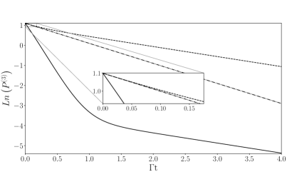
Figure 2: Mean number of atomic excitations, in logarithmic scale, as a function of time for the symmetric Dicke (solid line) and symmetric mixed (dashed line) initial state when $M=3$, $N=10$ and $\gamma_{c}=0.5\Gamma$. The case of independent emission of atoms, $\gamma_{c}=0$, (dashed-dotted) is plotted as a reference. For long times the sub-radiant decay dominates for both cases (symmetric Dicke and mixed states). For short times, the initially symmetric Dicke state is super-radiant, whereas for the initially symmetric mixed state the sub-radiant decay dominates (see inset).

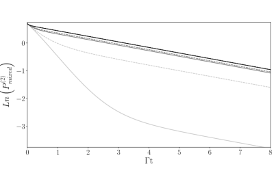
(a) Symmetric mixed state

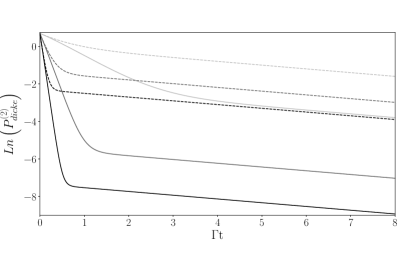
(b) symmetric Dicke state

Figure 3: Mean number of excited atoms, in logarithmic scale, as a function of time, calculated using perturbation theory (dashed line) and calculated without approximations (solid line). We use $\gamma_{c}=0.8\Gamma$ and $M=2$. We plot solutions for $N=2$ (light gray line), $N=8$ (dark gray line) and $N=20$ (black line). In (a) we compare solutions (157) and (264). In (b) we plot the expressions (164) and (263). Although the perturbed solutions were obtained for $\gamma_{c}\ll\Gamma$, they seem to be valid for $N\gg 1$.

7 Conclusions

The atomic damping basis is a powerful method to study the evolution of interacting atoms, when the system is symmetric under the interchange of atomic labels. Using this basis we obtained analytical expressions for the mean number of atomic excitations for the case of $M=1,2,3,4$ initially excited atoms, out of a total of $N$ atoms. Our results, that include the case where the initial state is not pure, show that the mean number of excited atoms decays as a sum of super- and sub- radiant exponentials. When there is atomic independent decay ($\Gamma\neq\gamma_{c}$) and at least two atoms are initially excited, the sub-radiant component of the evolution always appears in the solutions that we studied, and dominates the system evolution for large times.

Appendix A Some linear maps in terms of collective superoperators

The following are some useful identities between superoperators:

$$\begin{array}[]{ccc}\sum_{\mu}\hat{\sigma}_{-}^{(\mu)}\left|\rho\right)\hat{\sigma}_{+}^{(\mu)}=\breve{A}^{\mbox{\scriptsize$\begin{array}[]{cc}00\\ 11\end{array}$}}_{+}\left|\rho\right)&&\sum_{\mu}\hat{\sigma}_{+}^{(\mu)}\left|\rho\right)\hat{\sigma}_{-}^{(\mu)}=\breve{A}^{\mbox{\scriptsize$\begin{array}[]{cc}11\\ 00\end{array}$}}_{+}\left|\hat{\rho}\right)\\ \sum_{\mu}\hat{\sigma}_{+}^{(\mu)}\hat{\sigma}_{-}^{(\mu)}\left|\rho\right)=\left(\breve{A}^{\mbox{\scriptsize$\begin{array}[]{cc}10\\ 10\end{array}$}}_{+}+\breve{A}^{\mbox{\scriptsize$\begin{array}[]{cc}11\\ 11\end{array}$}}_{+}\right)\left|\rho\right)&&\sum_{\mu}\left|\rho\right)\hat{\sigma}_{+}^{(\mu)}\hat{\sigma}_{-}^{(\mu)}=\left(\breve{A}^{\mbox{\scriptsize$\begin{array}[]{cc}01\\ 01\end{array}$}}_{+}+\breve{A}^{\mbox{\scriptsize$\begin{array}[]{cc}11\\ 11\end{array}$}}_{+}\right)\left|\rho\right)\\ \sum_{\mu}\hat{\sigma}_{-}^{(\mu)}\hat{\sigma}_{+}^{(\mu)}\left|\rho\right)=\left(\breve{A}^{\mbox{\scriptsize$\begin{array}[]{cc}01\\ 01\end{array}$}}_{+}+\breve{A}^{\mbox{\scriptsize$\begin{array}[]{cc}00\\ 00\end{array}$}}_{+}\right)\left|\rho\right)&&\sum_{\mu}\left|\rho\right)\hat{\sigma}_{-}^{(\mu)}\hat{\sigma}_{+}^{(\mu)}=\left(\breve{A}^{\mbox{\scriptsize$\begin{array}[]{cc}10\\ 10\end{array}$}}_{+}+\breve{A}^{\mbox{\scriptsize$\begin{array}[]{cc}00\\ 00\end{array}$}}_{+}\right)\left|\rho\right)\\ \hat{J}_{+}\left|\rho\right)=\left(\breve{A}^{\mbox{\scriptsize$\begin{array}[]{cc}10\\ 00\end{array}$}}_{+}+\breve{A}^{\mbox{\scriptsize$\begin{array}[]{cc}11\\ 01\end{array}$}}_{+}\right)\left|\rho\right)&&\left|\rho\right)\hat{J}_{+}=\left(\breve{A}^{\mbox{\scriptsize$\begin{array}[]{cc}10\\ 11\end{array}$}}_{+}+\breve{A}^{\mbox{\scriptsize$\begin{array}[]{cc}00\\ 01\end{array}$}}_{+}\right)\left|\rho\right)\\ \hat{J}_{-}\left|\rho\right)=\left(\breve{A}^{\mbox{\scriptsize$\begin{array}[]{cc}00\\ 10\end{array}$}}_{+}+\breve{A}^{\mbox{\scriptsize$\begin{array}[]{cc}01\\ 11\end{array}$}}_{+}\right)\left|\rho\right)&&\left|\rho\right)\hat{J}_{-}=\left(\breve{A}^{\mbox{\scriptsize$\begin{array}[]{cc}11\\ 10\end{array}$}}_{+}+\breve{A}^{\mbox{\scriptsize$\begin{array}[]{cc}01\\ 00\end{array}$}}_{+}\right)\left|\rho\right)\end{array}$$

$$\begin{array}[]{c}\hat{J}_{-}\left|\rho\right)\hat{J}_{+}=\left(\breve{A}^{\mbox{\scriptsize$\begin{array}[]{cc}00\\ 10\end{array}$}}_{+}+\breve{A}^{\mbox{\scriptsize$\begin{array}[]{cc}01\\ 11\end{array}$}}_{+}\right)\left(\breve{A}^{\mbox{\scriptsize$\begin{array}[]{cc}10\\ 11\end{array}$}}_{+}+\breve{A}^{\mbox{\scriptsize$\begin{array}[]{cc}00\\ 01\end{array}$}}_{+}\right)\left|\rho\right)\\ \hat{J}_{+}\left|\rho\right)\hat{J}_{-}=\left(\breve{A}^{\mbox{\scriptsize$\begin{array}[]{cc}10\\ 00\end{array}$}}_{+}+\breve{A}^{\mbox{\scriptsize$\begin{array}[]{cc}11\\ 01\end{array}$}}_{+}\right)\left(\breve{A}^{\mbox{\scriptsize$\begin{array}[]{cc}11\\ 10\end{array}$}}_{+}+\breve{A}^{\mbox{\scriptsize$\begin{array}[]{cc}01\\ 00\end{array}$}}_{+}\right)\left|\rho\right)\end{array}$$

Appendix B Eigenvectors of $\breve{L}_{i}$ for 3 excitations.

We show the basis for a subspace of $N$ atoms with at most three excitations. In this approximation we consider zero all those eigenvectors with less than $N-3$ atoms in the state ground. The right eigenvectors of $\breve{L}_{i}$ ($\gamma_{10}=\Gamma-\gamma_{c}$) are

$$\lambda_{N-3,0}=-\frac{3\gamma_{10}}{2}:\left|N-3,0\right)_{0}=\frac{N(N-1)(N-2)}{6}\hat{Q}^{\mbox{\scriptsize$\begin{array}[]{cc}N&0\\ 0&0\end{array}$}},\quad\left|N-3,0\right)_{1}=\frac{N(N-1)(N-2)}{2}\hat{Q}^{\mbox{\scriptsize$\begin{array}[]{cc}N-3&2\\ 1&0\end{array}$}},$$ (176)

$$\left|N-3,0\right)_{2}=\frac{N(N-1)(N-2)}{2}\hat{Q}^{\mbox{\scriptsize$\begin{array}[]{cc}N-3&1\\ 2&0\end{array}$}},\quad\left|N-3,0\right)_{3}=\frac{N(N-1)(N-2)}{6}\hat{Q}^{\mbox{\scriptsize$\begin{array}[]{cc}N-3&0\\ 3&0\end{array}$}}$$ (181)

$$\lambda_{N-2,0}=-\gamma_{10}:\left|N-2,0\right)_{0}=\frac{N(N-1)}{3}\hat{Q}^{\mbox{\scriptsize$\begin{array}[]{cc}N-2&2\\ 0&0\end{array}$}},\quad\left|N-2,0\right)_{1}=N(N-1)\hat{Q}^{\mbox{\scriptsize$\begin{array}[]{cc}N-2&1\\ 1&0\end{array}$}},$$ (186)

$$\left|N-2,0\right)_{2}=\frac{N(N-1)}{2}\hat{Q}^{\mbox{\scriptsize$\begin{array}[]{cc}N-2&0\\ 2&0\end{array}$}}$$ (189)

$$\lambda_{N-2,1}=-2\gamma_{10}:\left|N-2,1\right)_{0}=-\frac{N(N-1)(N-2)}{2}\left(\hat{Q}^{\mbox{\scriptsize$\begin{array}[]{cc}N-2&2\\ 0&0\end{array}$}}-\hat{Q}^{\mbox{\scriptsize$\begin{array}[]{cc}N-3&2\\ 0&1\end{array}$}}\right),$$ (194)

$$\left|N-2,1\right)_{1}=-N(N-1)(N-2)\left(\hat{Q}^{\mbox{\scriptsize$\begin{array}[]{cc}N-2&1\\ 1&0\end{array}$}}-\hat{Q}^{\mbox{\scriptsize$\begin{array}[]{cc}N-3&1\\ 1&1\end{array}$}}\right),$$ (199)

$$\left|N-2,1\right)_{2}=-\frac{N(N-1)(N-2)}{2}\left(\hat{Q}^{\mbox{\scriptsize$\begin{array}[]{cc}N-2&0\\ 2&0\end{array}$}}-\hat{Q}^{\mbox{\scriptsize$\begin{array}[]{cc}N-3&0\\ 2&1\end{array}$}}\right)$$ (204)

$$\lambda_{N-1,0}=-\frac{\gamma_{10}}{2}:\left|N-1,0\right)_{0}=N\hat{Q}^{\mbox{\scriptsize$\begin{array}[]{cc}N-1&1\\ 0&0\end{array}$}},\qquad\left|N-1,0\right)_{1}=N\hat{Q}^{\mbox{\scriptsize$\begin{array}[]{cc}N-1&0\\ 1&0\end{array}$}}$$ (209)

$$\lambda_{N-1,1}=-\frac{3\gamma_{10}}{2}:\left|N-1,1\right)_{0}=-N(N-1)\left(\hat{Q}^{\mbox{\scriptsize$\begin{array}[]{cc}N-1&1\\ 0&0\end{array}$}}-\hat{Q}^{\mbox{\scriptsize$\begin{array}[]{cc}N-2&1\\ 0&1\end{array}$}}\right),$$ (214)

$$\left|N-1,1\right)_{1}=-N(N-1)\left(\hat{Q}^{\mbox{\scriptsize$\begin{array}[]{cc}N-1&0\\ 1&0\end{array}$}}-\hat{Q}^{\mbox{\scriptsize$\begin{array}[]{cc}N-2&0\\ 1&1\end{array}$}}\right)$$ (219)

$$\lambda_{N-1,2}=-\frac{5\gamma_{10}}{2}:\left|N-1,2\right)_{0}=\frac{N(N-1)(N-2)}{2}\left(\hat{Q}^{\mbox{\scriptsize$\begin{array}[]{cc}N-1&1\\ 0&0\end{array}$}}-2\hat{Q}^{\mbox{\scriptsize$\begin{array}[]{cc}N-2&1\\ 0&1\end{array}$}}+\hat{Q}^{\mbox{\scriptsize$\begin{array}[]{cc}N-3&1\\ 0&2\end{array}$}}\right),$$ (226)

$$\left|N-1,2\right)_{1}=\frac{N(N-1)(N-2)}{2}\left(\hat{Q}^{\mbox{\scriptsize$\begin{array}[]{cc}N-1&0\\ 1&0\end{array}$}}-2\hat{Q}^{\mbox{\scriptsize$\begin{array}[]{cc}N-2&0\\ 1&1\end{array}$}}+\hat{Q}^{\mbox{\scriptsize$\begin{array}[]{cc}N-3&0\\ 1&2\end{array}$}}\right)$$ (233)

$$\lambda_{N,0}=0:\left|N,0\right)_{0}=\hat{Q}^{\mbox{\scriptsize$\begin{array}[]{cc}N&0\\ 0&0\end{array}$}}$$ (236)

$$\lambda_{N,1}=-\gamma_{10}:\left|N,1\right)_{0}=-N\left(\hat{Q}^{\mbox{\scriptsize$\begin{array}[]{cc}N&0\\ 0&0\end{array}$}}-\hat{Q}^{\mbox{\scriptsize$\begin{array}[]{cc}N-1&0\\ 0&1\end{array}$}}\right)$$ (241)

$$\lambda_{N,2}=-2\gamma_{10}:\left|N,2\right)_{0}=\frac{N(N-1)}{2}\left(\hat{Q}^{\mbox{\scriptsize$\begin{array}[]{cc}N&0\\ 0&0\end{array}$}}-2\hat{Q}^{\mbox{\scriptsize$\begin{array}[]{cc}N-1&0\\ 0&1\end{array}$}}+\hat{Q}^{\mbox{\scriptsize$\begin{array}[]{cc}N-2&0\\ 0&2\end{array}$}}\right)$$ (248)

$$\lambda_{N,3}=-3\gamma_{10}:\left|N,3\right)_{0}=-\frac{N(N-1)(N-2)}{6}\left(\hat{Q}^{\mbox{\scriptsize$\begin{array}[]{cc}N&0\\ 0&0\end{array}$}}-3\hat{Q}^{\mbox{\scriptsize$\begin{array}[]{cc}N-1&0\\ 0&1\end{array}$}}+3\hat{Q}^{\mbox{\scriptsize$\begin{array}[]{cc}N-2&0\\ 0&2\end{array}$}}-\hat{Q}^{\mbox{\scriptsize$\begin{array}[]{cc}N-3&0\\ 0&3\end{array}$}}\right)$$ (257)

If we perturb the operator $\breve{L}_{i}$ with $\breve{L}_{c}$ we obtain, to first order in the eigenvalues $\Lambda_{n,m}$, and zero order in the right eigenvectors $\left|\phi_{n,m}\right)$, the following results:

$$\begin{array}[]{cccc}\Lambda_{0,1}=0:&\left|\phi_{0,1}\right)=\left|N,0\right)_{0}&\Lambda_{3,4}=-\frac{3}{2}\gamma_{10}\left(1+\frac{N-2}{3}\gamma_{c}\right):&\left|\phi_{3,4}\right)=-\frac{2}{N-2}\left|N-3,0\right)_{1}+\left|N-1,1\right)_{0}\\ \Lambda_{1,1}=-\frac{1}{2}\gamma_{10}\big{(}1+N\gamma_{c}\big{)}:&\left|\phi_{1,1}\right)=\left|N-1,0\right)_{0}&\Lambda_{3,5}=-\frac{3}{2}\gamma_{10}\left(1+\frac{3N-2}{3}\gamma_{c}\right):&\left|\phi_{3,5}\right)=\left|N-3,0\right)_{2}+\left|N-1,1\right)_{1}\\ \Lambda_{1,2}=-\frac{1}{2}\gamma_{10}\big{(}1+N\gamma_{c}\big{)}:&\left|\phi_{1,2}\right)=\left|N-1,0\right)_{1}&\Lambda_{3,6}=-\frac{3}{2}\gamma_{10}\left(1+\frac{N-2}{3}\gamma_{c}\right):&\left|\phi_{3,6}\right)=-\frac{2}{N-2}\left|N-3,0\right)_{2}+\left|N-1,1\right)_{1}\\ \Lambda_{2,1}=-\gamma_{10}\big{[}1+(N-1)\gamma_{c}\big{]}:&\left|\phi_{2,1}\right)=\left|N-2,0\right)_{0}&\Lambda_{4,1}=-2\gamma_{10}\left(1+\frac{N}{2}\gamma_{c}\right):&\left|\phi_{4,1}\right)=\left|N-2,1\right)_{0}\\ \Lambda_{2,2}=-\gamma_{10}\big{[}1+(N-1)\gamma_{c}\big{]}:&\left|\phi_{2,2}\right)=\left|N-2,0\right)_{2}&\Lambda_{4,2}=-2\gamma_{10}\left(1+\frac{N}{2}\gamma_{c}\right):&\left|\phi_{4,2}\right)=\left|N-2,1\right)_{2}\\ \Lambda_{2,3}=-\gamma_{10}\left(1+N\gamma_{c}\right):&\left|\phi_{2,3}\right)=\left|N-2,0\right)_{1}+\left|N,1\right)_{0}&\Lambda_{4,3}=-2\gamma_{10}\left(1+\frac{N+2+\nu}{4}\gamma_{c}\right):&\left|\phi_{4,3}\right)=\frac{N-2+\nu}{4N-8}\left|N-2,1\right)_{1}+\left|N,2\right)_{0}\\ \Lambda_{2,4}=-\gamma_{10}:&\left|\phi_{2,4}\right)=-\frac{1}{N-1}\left|N-2,0\right)_{1}+\left|N,1\right)_{0}&\Lambda_{4,4}=-2\gamma_{10}\left(1+\frac{N+2-\nu}{2}\gamma_{c}\right):&\left|\phi_{4,4}\right)=\frac{N-2-\nu}{4N-8}\left|N-2,1\right)_{1}+\left|N,2\right)_{0}\\ \Lambda_{3,1}=-\frac{3}{2}\gamma_{10}\big{[}1+(N-2)\gamma_{c}\big{]}:&\left|\phi_{3,1}\right)=\left|N-3,0\right)_{0}&\Lambda_{5,1}=-\frac{5}{2}\gamma_{10}\big{(}1+\frac{N+4}{5}\gamma_{c}\big{)}:&\left|\phi_{5,1}\right)=\left|N-1,2\right)_{0}\\ \Lambda_{3,2}=-\frac{3}{2}\gamma_{10}\big{[}1+(N-2)\gamma_{c}\big{]}:&\left|\phi_{3,2}\right)=\left|N-3,0\right)_{3}&\Lambda_{5,2}=-\frac{5}{2}\gamma_{10}\big{(}1+\frac{N+4}{5}\gamma_{c}\big{)}:&\left|\phi_{5,2}\right)=\left|N-1,2\right)_{1}\\ \Lambda_{3,3}=-\frac{3}{2}\gamma_{10}\left(1+\frac{3N-2}{3}\gamma_{c}\right):&\left|\phi_{3,3}\right)=\left|N-3,0\right)_{1}+\left|N-1,1\right)_{0}&\Lambda_{6,1}=-3\gamma_{10}\big{(}1+\gamma_{c}\big{)}:&\left|\phi_{6,1}\right)=\left|N,3\right)_{0}\end{array}$$

with $\nu=\sqrt{(N+6)(N-2)}$. Note that the eigenvalues remain degenerate at first order.

With this basis we can solve Equation (8) for states (151) and (162). As an example, for $M=3$ we get

$$\left|\rho^{(3)}(t)\right)=\left|\phi_{0,1}\right)+\frac{3k_{1}\,e^{-\left(\gamma_{10}+N\gamma_{c}\right)t}}{N^{2}}\left|\phi_{2,3}\right)+\frac{3k_{2}\,e^{-\gamma_{10}t}}{N^{2}}\left|\phi_{2,4}\right)+\frac{3k_{3}\,e^{-2\left(\gamma_{10}+\frac{N+2+\sqrt{(N+6)(N-2)}}{4}\gamma_{c}\right)t}}{N(N-1)}\left|\phi_{4,3}\right)$$

$$+\frac{3k_{4}\,e^{-2\left(\gamma_{10}+\frac{N+2-\sqrt{(N+6)(N-2)}}{4}\gamma_{c}\right)t}}{N(N-1)}\left|\phi_{4,4}\right)+\frac{6e^{-3\left(\gamma_{10}+\gamma_{c}\right)t}}{N(N-1)(N-2)}\left|\phi_{6,1}\right)\,,$$ (258)

where for mixed states we have

$$k_{1} = 1,\qquad k_{2}=N-1,\qquad k_{3}=\frac{N+6-\sqrt{(N+6)(N-2)}}{N+6},$$

$$k_{4} = \frac{N+6+\sqrt{(N+6)(N-2)}}{N+6}\,,$$ (259)

and for symmetric Dicke states the coefficients are

$$k_{1} = N-2,\qquad k_{2}=2,\qquad k_{3}=\frac{3N-10+\sqrt{(N+6)(N-2)}}{\sqrt{(N+6)(N-2)}},$$

$$k_{4} = -\frac{3N-10-\sqrt{(N+6)(N-2)}}{\sqrt{(N+6)(N-2)}}\,.$$ (260)

We observe sub- and super-radiant terms due to interaction between the atoms.

Appendix C Damping basis without perturbation for a system with three excitations.

If we consider three excited atoms among a total of $N$, the linear map $\breve{L}_{i}+\breve{L}_{c}$ is closed for the ordered set $\mathcal{A}_{3}=\{\left|N,0\right)_{0},\left|N,1\right)_{0},\left|N-2,0\right)_{1},\left|N,2\right)_{0},\left|N-2,1\right)_{1},$ $\left|N-4,0\right)_{2},\left|N,3\right)_{0},\left|N-2,2\right)_{1},\left|N-4,1\right)_{2},\left|N-6,0\right)_{3}\}$. The matrix form of the superoperator in this subspace is

$$-\left(\begin{array}[]{cccccccccc}0&0&0&0&0&0&0&0&0&0\\ 0&\gamma_{10}+\gamma_{c}&(N-1)\gamma_{c}&0&0&0&0&0&0&0\\ 0&\gamma_{c}&\gamma_{10}+(N-1)\gamma_{c}&-2\gamma_{c}&-2(N-2)\gamma_{c}&0&0&0&0&0\\ 0&0&0&2\gamma_{10}+2\gamma_{c}&2(N-2)\gamma_{c}&0&0&0&0&0\\ 0&0&0&\gamma_{c}&2\gamma_{10}+N\gamma_{c}&(N-3)\gamma_{c}&-2\gamma_{c}&-2(N-3)\gamma_{c}&0&0\\ 0&0&0&0&4\gamma_{c}&2\gamma_{10}+2(N-3)\gamma_{c}&0&-8\gamma_{c}&-4(N-4)\gamma_{c}&0\\ 0&0&0&0&0&0&3\gamma_{10}+3\gamma_{c}&3(N-3)\gamma_{c}&0&0\\ 0&0&0&0&0&0&\gamma_{c}&3\gamma_{10}+(N+1)\gamma_{c}&2(N-4)\gamma_{c}&0\\ 0&0&0&0&0&0&0&4\gamma_{c}&3\gamma_{10}+(2N-5)\gamma_{c}&(N-5)\gamma_{c}\\ 0&0&0&0&0&0&0&0&9\gamma_{c}&3\gamma_{10}+3(N-5)\gamma_{c}\end{array}\right)$$

By diagonalizing this matrix we get analytic expressions for the eigenvectors and the eigenvalues that allow us to obtain the evolution of the states (151) and (162) without perturbation and for $M=1,\,2,\,3$.

Appendix D Population of excited atoms

The mean number of excited atoms $P^{(M)}$, as a function of time, is shown below for $M=1,2,3$ excitations, and for initially symmetric mixed states (151) and symmetric Dicke states (162). Using $\gamma_{10}=\Gamma-\gamma_{c}$ we obtain:

$$P_{\textrm{dicke}}^{(1)}(t)=e^{-\left[\Gamma+(N-1)\gamma_{c}\right]t}\,,$$ (261)

$$P_{\textrm{mixed}}^{(1)}(t)=\frac{N-1}{N}e^{-\left(\Gamma-\gamma_{c}\right)t}+\frac{1}{N}e^{-\left[\Gamma+(N-1)\gamma_{c}\right]t}\,,$$ (262)

$$P_{\textrm{dicke}}^{(2)}(t)=\frac{2}{N\left[\gamma_{10}+(N-2)\gamma_{c}\right]\left[\gamma_{10}+2(N-1)\gamma_{c}\right]}\bigg{[}\left\{(N-2)\gamma_{10}\gamma_{c}+\gamma_{10}^{2}\right\}e^{-\left(\Gamma-\gamma_{c}\right)t}+\bigg{\{}\gamma_{10}\gamma_{c}\left(3N^{2}-5N+2\right)$$

$$+(N-1)\gamma_{10}^{2}+2N(N-1)^{2}\gamma_{c}^{2}\bigg{\}}e^{-\left[\Gamma+(N-1)\gamma_{c}\right]t}-2N(N-1)\gamma_{c}^{2}e^{-2\left[\Gamma+(N-2)\gamma_{c}\right]t}\bigg{]}\,,$$ (263)

$$P_{\textrm{mixed}}^{(2)}(t)=2\Bigg{[}\left(\frac{N-1}{N}-\frac{2\gamma_{c}\left[\gamma_{10}+2(N-2)\gamma_{c}\right]}{N\left[\gamma_{10}+(N-2)\gamma_{c}\right]\left[\gamma_{10}+2(N-1)\gamma_{c}\right]}\right)e^{-\left(\Gamma-\gamma_{c}\right)t}+\left(\frac{1}{N}+\frac{2\gamma_{c}\left[\gamma_{10}+(N-4)\gamma_{c}\right]}{N\left[\gamma_{10}-2\gamma_{c}\right]\left[\gamma_{10}+(N-2)\gamma_{c}\right]}\right)e^{-\left[\Gamma+(N-1)\gamma_{c}\right]t}$$

$$-\frac{4\gamma_{c}^{2}e^{-2\left[\Gamma+(N-2)\gamma_{c}\right]t}}{N\left[\gamma_{10}+(N-2)\gamma_{c}\right]\left[\gamma_{10}+2(N-1)\gamma_{c}\right]}-\frac{2(N-2)\gamma_{c}^{2}e^{-\left[2\Gamma+(N-4)\gamma_{c}\right]t}}{N\left[\gamma_{10}-2\gamma_{c}\right]\left[\gamma_{10}+(N-2)\gamma_{c}\right]}\Bigg{]}\,,$$ (264)

$$P_{\textrm{dicke}}^{(3)}(t)=3\Bigg{[}\frac{4(N-2)\gamma_{c}^{3}\left[\gamma_{10}+3(N-2)\gamma_{c}\right]e^{-\left[3\Gamma+(3N-7)\gamma_{c}\right]}}{\left[\gamma_{10}+(N-4)\gamma_{c}\right]\left[\gamma_{10}+(N-3)\gamma_{c}\right]\left[\gamma_{10}+2(N-2)\gamma_{c}\right]\left[2\gamma_{10}+3(N-2)\gamma_{c}\right]}-\frac{4\gamma_{10}(N-2)\gamma_{c}^{2}e^{-\left[2\Gamma+(N-4)\gamma_{c}\right]t}}{N\left[\gamma_{10}-2\gamma_{c}\right]\left[\gamma_{10}+(N-2)\gamma_{c}\right]\left[\gamma_{10}+2(N-2)\gamma_{c}\right]}$$

$$-\frac{4(N-2)(N-1)\left(\gamma_{10}+N\gamma_{c}\right)\gamma_{c}^{2}e^{-2\left[\Gamma+(N-2)\gamma_{c}\right]t}}{N\left[\gamma_{10}+(N-4)\gamma_{c}\right]\left[\gamma_{10}+(N-2)\gamma_{c}\right]\left[\gamma_{10}+2(N-1)\gamma_{c}\right]}+\frac{2\gamma_{10}\left(2\gamma_{10}^{2}+(5N-6)\gamma_{10}\gamma_{c}+(N-2)(3N-4)\gamma_{c}^{2}\right)e^{-\left(\Gamma-\gamma_{c}\right)t}}{N\left[\gamma_{10}+(N-2)\gamma_{c}\right]\left[2\gamma_{10}+3(N-2)\gamma_{c}\right]\left[\gamma_{10}+2(N-1)\gamma_{c}\right]}+$$

$$\frac{(N-2)\left(\gamma_{10}^{3}+(2N-3)\gamma_{10}^{2}\gamma_{c}+(N-4)(N-1)\gamma_{10}\gamma_{c}^{2}-2N(N-1)\gamma_{c}^{3}\right)e^{-\left[\Gamma+(N-1)\gamma_{c}\right]t}}{N\left[\gamma_{10}-2\gamma_{c}\right]\left[\gamma_{10}+(N-3)\gamma_{c}\right]\left[\gamma_{10}+(N-2)\gamma_{c}\right]}\Bigg{]}\,,$$ (265)

$$P_{\textrm{mixed}}^{(3)}=3\Bigg{[}\frac{4(N-4)(N-3)\gamma_{c}^{3}e^{-\left[3\Gamma+(N-7)\gamma_{c}\right]t}}{(N-2)(N-1)\left[\gamma_{10}-2\gamma_{c}\right]^{2}\left[2\gamma_{10}+(N-4)\gamma_{c}\right]}+\frac{16(N-3)\left[\gamma_{10}+(N-6)\gamma_{c}\right]\gamma_{c}^{3}e^{-\left[3\Gamma+(2N-9)\gamma_{c}\right]t}}{N(N-2)\left[\gamma_{10}-4\gamma_{c}\right]\left[2\gamma_{10}+(N-6)\gamma_{c}\right]\left[\gamma_{10}+(N-4)\gamma_{c}\right]\left[\gamma_{10}+(N-3)\gamma_{c}\right]}$$

$$+\frac{24\left[\gamma_{10}+3(N-2)\gamma_{c}\right]\gamma_{c}^{3}e^{-3\left[\Gamma+(N-3)\gamma_{c}\right]t}}{N(N-1)\left[\gamma_{10}+(N-4)\gamma_{c}\right]\left[\gamma_{10}+(N-3)\gamma_{c}\right]\left[\gamma_{10}+2(N-2)\gamma_{c}\right]\left[2\gamma_{10}+3(N-2)\gamma_{c}\right]}-$$

$$\frac{8\left[\gamma_{10}^{2}+(N-4)\gamma_{c}\gamma_{10}-12\gamma_{c}^{2}\right]\gamma_{c}^{2}e^{-2\left[\Gamma+(N-2)\gamma_{c}\right]t}}{N\left[\gamma_{10}-4\gamma_{c}\right]\left[\gamma_{10}+(N-4)\gamma_{c}\right]\left[\gamma_{10}+(N-2)\gamma_{c}\right]\left[\gamma_{10}+2(N-1)\gamma_{c}\right]}-$$

$$\frac{4\left[(N-2)\gamma_{10}^{3}+[12+N(3N-14)]\gamma_{c}\gamma_{10}^{2}+2\{N[14+N(N-8)]+4\}\gamma_{c}^{2}\gamma_{10}-8(N-3)(N-2)\gamma_{c}^{3}\right]\gamma_{c}^{2}e^{-\left[2\Gamma+(N-4)\gamma_{c}\right]t}}{N\left[\gamma_{10}-2\gamma_{c}\right]^{2}\left[\gamma_{10}+(N-4)\gamma_{c}\right]\left[\gamma_{10}+(N-2)\gamma_{c}\right]\left[\gamma_{10}+2(N-2)\gamma_{c}\right]}+$$

$$\frac{\left[2\gamma_{10}^{5}+(5N-16)\gamma_{c}\gamma_{10}^{4}+[26+N(4N-27)]\gamma_{c}^{2}\gamma_{10}^{3}+\{N[12+N(N-11)]+44\}\gamma_{c}^{3}\gamma_{10}^{2}-8[3+N(N-7)]\gamma_{c}^{4}\gamma_{10}+24(N-6)\gamma_{c}^{5}\right]}{N\left[\gamma_{10}-2\gamma_{c}\right]^{2}\left[2\gamma_{10}+(N-6)\gamma_{c}\right]\left[\gamma_{10}+(N-3)\gamma_{c}\right]\left[\gamma_{10}+(N-2)\gamma_{c}\right]}$$

$$\times e^{-\left[\Gamma+(N-1)\gamma_{c}\right]t}+\frac{e^{-\left(\Gamma-\gamma_{c}\right)t}}{N\left[2\gamma_{10}+(N-4)\gamma_{c}\right]\left[\gamma_{10}+(N-3)\gamma_{c}\right]\left[\gamma_{10}+(N-2)\gamma_{c}\right]\left[2\gamma_{10}+3(N-2)\gamma_{c}\right]\left[\gamma_{10}+2(N-1)\gamma_{c}\right]}\Bigg{(}4(N-1)\gamma_{10}^{5}$$

$$+8[3N(N-3)+4]\gamma_{c}\gamma_{10}^{4}+\{N[5N(11N-57)+378]-52\}\gamma_{c}^{2}\gamma_{10}^{3}+6(N-4)(N-3)(N-2)\left(N^{3}-4N^{2}+N-2\right)\gamma_{c}^{5}+$$

$$(N\{3N[N(20N-151)+357]-730\}-88)\gamma_{c}^{3}\gamma_{10}^{2}+(N-3)(N\{N[N(31N-221)+446]-192\}-16)\gamma_{c}^{4}\gamma_{10}\Bigg{)}\Bigg{]}\,.$$ (266)

References

References

• [1] Briegel H J and Englert B G 1993 Phys. Rev. A 47(4) 3311–3329
• [2] Pichler H, Ramos T, Daley A J and Zoller P 2015 Phys. Rev. A 91(4) 042116
• [3] Lund-Hansen T, Stobbe S, Julsgaard B, Thyrrestrup H, Sünner T, Kamp M, Forchel A and Lodahl P 2008 Phys. Rev. Lett. 101(11) 113903
• [4] Goban A, Hung C L, Hood J D, Yu S P, Muniz J A, Painter O and Kimble H J 2015 Phys. Rev. Lett. 115(6) 063601
• [5] Chang D E, Sørensen A S, Hemmer P R and Lukin M D 2007 Phys. Rev. B 76(3) 035420
• [6] Lehmberg R H 1970 Phys. Rev. A 2(3) 883–888
• [7] Agarwal G S 1970 Phys. Rev. A 2(5) 2038–2046
• [8] Clemens J P, Horvath L, Sanders B C and Carmichael H J 2003 Phys. Rev. A 68(2) 023809
• [9] Svidzinsky A and Chang J T 2008 Phys. Rev. A 77(4) 043833
• [10] Le Kien F, Gupta S D, Nayak K P and Hakuta K Phys. Rev. A 72(6) 063815
• [11] Solano P, Barberis-Blostein P, Fatemi F K, Orozco L A and Rolston S L 2017 Nature Communications 8 1857
• [12] Vetsch E, Reitz D, Sagué G, Schmidt R, Dawkins S T and Rauschenbeutel A 2010 Phys. Rev. Lett. 104(20) 203603
• [13] Chang D E, Jiang L, Gorshkov A V and Kimble H J 2012 New Journal of Physics 14 063003
• [14] González-Tudela A, Paulisch V, Kimble H J and Cirac J I 2017 Phys. Rev. Lett. 118(21) 213601
• [15] Clemens J P and Carmichael H J 2002 Phys. Rev. A 65(2) 023815
• [16] Lehmberg R H 1970 Phys. Rev. A 2(3) 889
• [17] Mokhlespour S, Haverkort J E M, Slepyan G, Maksimenko S and Hoffmann A 2012 Phys. Rev. B 86(24) 245322
• [18] Emary C and Brandes T 2003 Phys. Rev. E 67(6) 066203
• [19] Hayn M, Emary C and Brandes T 2011 Phys. Rev. A 84(5) 053856
• [20] Wall M L, Safavi-Naini A and Rey A M 2016 Phys. Rev. A 94(5) 053637
• [21] Glauber R J and Haake F 1976 Phys. Rev. A 13(1) 357–366
• [22] Xu M, Tieri D A and Holland M J 2013 Phys. Rev. A 87(6) 062101
• [23] Chase B A and Geremia J M 2008 Phys. Rev. A 78(5) 052101
• [24] Gegg M and Richter M 2017 Scientific Reports 7 16304
• [25] Shammah N, Ahmed S, Lambert N, De Liberato S and Nori F 2018 Phys. Rev. A 98(6) 063815
• [26] Bolaños M and Barberis-Blostein P 2015 Journal of Physics A: Mathematical and Theoretical 48 445301
• [27] Bienert M and Barberis-Blostein P 2015 Phys. Rev. A 91(2) 023818
• [28] Bienert M, Torres J M, Zippilli S and Morigi G 2007 Phys. Rev. A 76(1) 013410
• [29] Torres J M, Betzholz R and Bienert M 2019 Journal of Physics A: Mathematical and Theoretical 52 08LT02
• [30] Pielawa S, Davidovich L, Vitali D and Morigi G 2010 Phys. Rev. A 81(4) 043802
• [31] Tarasov V 2008 Quantum Mechanics of Non-Hamiltonian and Dissipative Systems Monograph Series on Nonlinear Science and Complexity (Elsevier)
• [32] Kien F L and Hakuta K 2008 Phys. Rev. A 77(1) 013801
• [33] Le-Kien F y Rauschenbeutel A 2014 Phys. Rev. A 90(6) 063816
• [34] Hartmann S 2016 Quantum Info. Comput. 16 1333–1348
• [35] Sakurai J 1994 Modern Quantum Mechanics. Revised Edition (Addison-Wesley)
• [36] Hall B 2013 Quantum Theory for Mathematicians Graduated Text in Mathematics (Springer)
• [37] Horn R A y Johnson C R 2012 Matrix Analysis 2nd ed (New York, NY, USA: Cambridge University Press)
• [38] Vetsch E, Reitz D, Sagué G, Schmidt R, Dawkins S T and Rauschenbeutel A 2010 Phys. Rev. Lett. 104(20) 203603
• [39] Carmichael H 1993 An Open Systems Approach to Quantum Optics (Springer-Verlag)
• [40] Goban A, Hung C L, Hood J D, Yu S P, Muniz J A, Painter O and Kimble H J 2015 Phys. Rev. Lett. 115(6) 063601
• [41] Arcari M, Söllner I, Javadi A, Lindskov Hansen S, Mahmoodian S, Liu J, Thyrrestrup H, Lee E H, Song J D, Stobbe S and Lodahl P 2014 Phys. Rev. Lett. 113(9) 093603