The large scale polarization explorer (LSPE) for CMB measurements: performance forecast

Abstract

The measurement of the polarization of the Cosmic Microwave Background (CMB) radiation is one of the current frontiers in cosmology. In particular, the detection of the primordial divergence-free component of the polarization field, the B-mode, could reveal the presence of gravitational waves in the early Universe. The detection of such a component is at the moment the most promising technique to probe the inflationary theory describing the very early evolution of the Universe. We present the updated performance forecast of the Large Scale Polarization Explorer (LSPE), a program dedicated to the measurement of the CMB polarization. LSPE is composed of two instruments: LSPE-Strip, a radiometer-based telescope on the ground in Tenerife-Teide observatory, and LSPE-SWIPE (Short-Wavelength Instrument for the Polarization Explorer) a bolometer-based instrument designed to fly on a winter arctic stratospheric long-duration balloon. The program is among the few dedicated to observation of the Northern Hemisphere, while most of the international effort is focused into ground-based observation in the Southern Hemisphere. Measurements are currently scheduled in Winter 2022/23 for LSPE-SWIPE, with a flight duration up to 15 days, and in Summer 2022 with two years observations for LSPE-Strip. We describe the main features of the two instruments, identifying the most critical aspects of the design, in terms of impact on the performance forecast. We estimate the expected sensitivity of each instrument and propagate their combined observing power to the sensitivity to cosmological parameters, including the effect of scanning strategy, component separation, residual foregrounds and partial sky coverage. We also set requirements on the control of the most critical systematic effects and describe techniques to mitigate their impact. LSPE will reach a sensitivity in tensor-to-scalar ratio of $\sigma_{r}<0.01$, set an upper limit $r<0.015$ at 95% confidence level, and improve constraints on other cosmological parameters.

1 Introduction

The Large Scale Polarization Explorer (LSPE) is designed to measure the polarization of the Cosmic Microwave Background (CMB) at large angular scales, and in particular to constrain the curl component of CMB polarization (B-mode). This is produced by tensor perturbations generated during cosmic inflation in the very early Universe [1, 2]. The level of this signal is unknown: current inflation models are unable to provide a firm reference value. However, the detection of this signal would be of utmost importance, providing a way to measure the energy-scale of inflation and a window on the physics at extremely high energies. While the level of CMB temperature anisotropy is of the order of $100\text{\thinspace}\mathrm{\SIUnitSymbolMicro K}$ r.m.s. and the level of the gradient component of CMB polarization (E-mode generated by scalar - density perturbations) is of the order of $3\text{\thinspace}\mathrm{\SIUnitSymbolMicro K}$, the current upper limits for the level of B-mode polarization are a fraction of $\text{\thinspace}\mathrm{\SIUnitSymbolMicro K}$, corresponding to a ratio between the amplitude of tensor perturbations and the amplitude of scalar perturbations (tensor-to-scalar ratio) $r<0.044$ at 95% confidence level, combining data from the Planck satellite and the BICEP/Keck ground telescopes [3, 4, 5]. The B-mode of inflationary origin is observable at large angular scales, greater than 1.5^∘.

The main scientific target of LSPE is to improve this limit. This and the additional scientific targets of the mission are reported in the following list:

• a detection of B-mode of CMB polarization at a level corresponding to a tensor-to-scalar ratio $r=0.03$ with 99.7% confidence level (CL); or an upper limit to tensor-to-scalar ratio $r=0.015$ at 95% CL;

• an improved measurement of the optical depth to the cosmic microwave background $\tau$, measured from the large scale E-mode CMB polarization; a measurement of $\tau$ is also critical to constraints on the sum of neutrino masses, from large-scale-structure probes [6, 7];

• investigation of the so called low-$\ell$ anomalies, a series of anomalies observed in the large angular scales of the CMB polarization, including lack of power on the largest angular scales, asymmetries and alignment of multipole moments;

• wide maps of foreground polarization produced in our galaxy by synchrotron emission and interstellar dust emission, which will be important to mapping the magnetic field in our Galaxy and to studying the properties of the ionized gas and of the diffuse interstellar dust in the Milky Way;

• improved limits or detection of cosmic birefringence;

• an improved measurement of the quality of the atmosphere at Teide Observatory (Tenerife) for CMB polarization measurements.

The observational cosmology community is carrying on a global effort to improve the measurement of the CMB polarization, aiming at a detection, or an improved upper limit, on the tensor-to-scalar ratio $r$. A list of the main experiments observing CMB polarization at large scales includes: the BICEP/Keck array program [8, 9] deployed at South Pole, aiming at improving the current upper limit (multipole range $21<\ell<335$); CLASS [10], in operation in the Atacama, aiming at detecting $r=0.01$ ($2<\ell<200$); Polarbear-2/Simons Array [11], beginning operations in the Atacama, aiming at $\sigma(r)=0.006$ if $r=0.1$ ($30<\ell<3000$); SPT-Pol [12], operated at the South Pole, measured $r<0.44$ at 95% c.l. ($52<\ell<2301$) and the third SPT generation SPT-3G [13], aiming at $\sigma(r)=0.01$ ($50<\ell<11000$); ACT [14, 15], operated in the Atacama, providing relevant constraints at smaller angular scales ($225<\ell<8725$); Simons Observatory [16], in preparation in the Atacama for early 2020s, aiming at $\sigma(r)=0.003$ ($30<\ell<8000$); GroundBIRD [17], in preparation in the Tenerife-Teide observatory, aiming at $\sigma(r)\simeq 0.01$ ($6<\ell<300$); QUBIC [18], in preparation for installation in Alto Chorrillos (Argentina, altitude 4869 m a.s.l), aiming at $\sigma(r)=0.021$ ($30<\ell<200$); CMB-S4 [19], in preparation for ground-based observations in 2027, aiming at detecting $r>0.003$ at greater than 5$\sigma$, or $r<0.001$ at 95% c.l.; SPIDER [20], balloon-based, waiting for the second flight, aiming at detecting $r>0.03$ at 99.7% c.l. ($2<\ell<200$); PIPER [21], balloon-based, aiming at constraining $r<0.007$ after 8 flights; PICO [22], a satellite-based instrument currently in study phase aiming at detection of $r=5\times 10^{-4}$ at 5$\sigma$ c.l. (full sky); and LiteBIRD [23, 24], which is currently the only approved satellite-based mission, planned for a launch in early 2028, aiming at $\delta r<0.001$, where $\delta r$ is the total error on $r$, including statistical, systematic error, and margin ($2<\ell<200$).

The overall design of the LSPE program has largely evolved since its first proposal [25, 26, 27, 28], and this paper presents its final design and expected performance. Section 2 describes the two instruments in detail; section 3 reports the expected instrumental sensitivities; section 4 describes the major systematic effects, mitigation techniques and calibration; section 5 presents the methods used in the foreground cleaning and likelihood evaluation and reports the expected performances on cosmological parameters. Finally, section 6 draws conclusions.

2 The instruments

Since the expected B-mode signal is smaller than the polarized foreground from our Galaxy, a wide frequency coverage is needed to monitor precisely the foregrounds at frequencies where they are most important, and to subtract them, in order to estimate the cosmological part of the detected B-mode signal. For the synchrotron foreground, prominent at frequencies below $\sim 100\text{\thinspace}\mathrm{GHz}$, where atmospheric transmission and noise are favorable, a ground based instrument is the most effective strategy, while for the CMB and the interstellar dust foreground, prominent at higher frequencies, a stratospheric balloon mission is preferred. For this reason, the LSPE program is based on the combination of two independent instruments: the Strip ground-based telescope, observing at $44\text{\thinspace}\mathrm{GHz}$, plus a $95\text{\thinspace}\mathrm{GHz}$ channel for atmospheric measurements, to be implemented at the Teide Observatory (Tenerife); and the SWIPE balloon-borne mission, observing at 145, 210 and $240\text{\thinspace}\mathrm{GHz}$ in a winter arctic stratospheric flight.

Table 1 reports basic parameters for the two instruments, in the baseline configuration. Map sensitivity is an approximated value, computed as the square root of $\sigma^{2}_{Q,U}=p\thinspace\text{NET}^{2}\thinspace{4\pi f_{\text{sky}}}/(T_{\text{obs}}N_{\text{det}})$, where $p=1$ for Strip and $p=2$ for SWIPE, to take into account that each SWIPE detector is instantaneously sensitive to one polarization only, $T_{\text{obs}}$ is the effective integration time, NET is the noise equivalent temperature of each detector, $f_{sky}$ is the observed sky fraction, and $N_{\text{det}}$ is the number of detectors. The power spectrum of the noise in polarization can be approximated by $\mathcal{N}^{E,B}_{\ell}=\sigma^{2}_{Q,U}/f_{\text{sky,cmb}}$, where $f_{\text{sky,cmb}}$ is the sky fraction used for CMB analysis, after masking the Galactic plane. More accurate performance is estimated using the instrument simulators, component separation, and cosmological parameters extraction algorithms, as described in sections 3 and 5.

Instrument	Strip		SWIPE
Site	Tenerife		balloon
Freq (GHz)	43	95	145	210	240
Bandwidth	17%	8%	30%	20%	10%
Angular resolution FWHM	20′	10′	85′
Field of view	$\pm 5^{\circ}$		$\pm 11^{\circ}$
Detector technology	HEMT		Multi-moded TES
Number of polarimeters (Strip) / detectors (SWIPE)	49	6	162	82	82
NET ($\text{\thinspace}\mathrm{\SIUnitSymbolMicro}\mathrm{K}_{CMB}\thinspace\mathrm{s}^{1/2}$)	515	1139	12.6	15.6	31.4
Observation time	$2\text{\thinspace}\mathrm{y}\mathrm{e}\mathrm{a}\mathrm{r}\mathrm{s}$		8 – $15\text{\thinspace}\mathrm{d}\mathrm{a}\mathrm{y}\mathrm{s}$
Observing efficiency	50%1		90%
Sky coverage2 (nominal) $f_{\text{sky,0}}$	28%		38%
Sky coverage2 (this paper) $f_{\text{sky}}$	50%		38%
Masked sky coverage for CMB analysis $f_{\text{sky,cmb}}$	25%		25%
Map sensitivity (nominal) $\sigma_{Q,U,0}$ ($\text{\thinspace}\mathrm{\SIUnitSymbolMicro}\mathrm{K}_{CMB}\thinspace\mathrm{a}\mathrm{r}\mathrm{c}\mathrm{m}\mathrm{i}\mathrm{n}$)	102	777	10	17	34
Map sensitivity (this paper) $\sigma_{Q,U}$ ($\text{\thinspace}\mathrm{\SIUnitSymbolMicro}\mathrm{K}_{CMB}\thinspace\mathrm{a}\mathrm{r}\mathrm{c}\mathrm{m}\mathrm{i}\mathrm{n}$)	130	990	10	17	34
Noise power spectrum $(\mathcal{N}^{E,B}_{\ell})^{1/2}$ ($\text{\thinspace}\mathrm{\SIUnitSymbolMicro}\mathrm{K}_{CMB}\thinspace\mathrm{a}\mathrm{r}\mathrm{c}\mathrm{m}\mathrm{i}\mathrm{n}$)	260	1980	20	34	68
1We estimate as 50% the time dedicated to sky observations, including calibration sources. We split the remaining 50% as follows: (i) 15% of lost time due to bad weather, (ii) 15% of unusable data when the Sun will have an angular distance from the nearest feed less than 10∘ [29], 20% of time dedicated to relative calibration (see section 4.2).
2 We consider two cases for Strip coverage, the nominal case with zenith angle $\beta_{\text{nominal}}=20$∘, and the case specific to this paper with zenith angle $\beta=35$∘, which maximise s the overlap as discussed in section 2.1 and illustrated in figure 2.

Table 1: LSPE baseline instrumental parameters. Details are reported in tables 2 and 4.

2.1 Observation strategy and sky coverage

Figure 1 illustrates the observation strategies for the two instruments. The Strip telescope will scan the sky at a constant zenith angle $\beta$ with $\omega_{\text{telescope}}=$1\text{\thinspace}\mathrm{r}\thinspace\mathrm{p}\thinspace\mathrm{m}\thinspace$$ spin rate. With this strategy, the observations cover a strip in equatorial declination $\delta$ ranging $\text{lat}_{\text{telescope}}-\beta<\delta<\text{lat}_{\text{telescope}}+\beta$, where $\text{lat}_{\text{telescope}}=$$$ N. This strategy minimizes atmospheric effects and, in combination with Earth rotation, to cover a large sky fraction.

The SWIPE observation strategy consists in continuous spinning of the payload, around the local zenith axis (spin axis), at fixed angular velocity $\omega_{\text{payload}}$. This is combined with steps in telescope zenith angle $\beta$ (a few steps per day), to cover an altitude range from 35^∘to 55^∘. The Earth rotation, combined with the drift of the payload around the Arctic, ensures a slow precession of the vertical spin axis around the Equatorial North Pole (precession axis). Precession angle $\alpha_{\text{p}}$ (co-latitude) and precession angular velocity $\omega_{\text{Earth}}$ are not exactly defined, due the partially random motion of the balloon, drifted by stratospheric winds. This strategy is combined with a Half-Wave Plate (HWP) based polarization modulator continuously spinning at rate $f_{\text{HWP}}$. The optimal payload spinning velocity and HWP rate are derived in Appendix A from detectors time constant and telescope angular response, and are found to be $\omega_{\text{payload}}\simeq$0.7\text{\thinspace}\mathrm{\SIUnitSymbolDegree}\thinspace\mathrm{s}^{-1}$$ and $f_{\text{HWP}}=0.5$ Hz. If the latitude remains constant, the observation covers a strip in equatorial declination $\delta$ in the range $$$-(\alpha_{\text{p}}+\beta_{\text{max}})<\delta<$$-(\beta_{\text{min}}-\alpha_{\text{p}})$ (see figure 1). The values of $\beta_{\text{min}}$ and $\beta_{\text{max}}$ also take into account the wide field of view $\pm 10^{\circ}$.

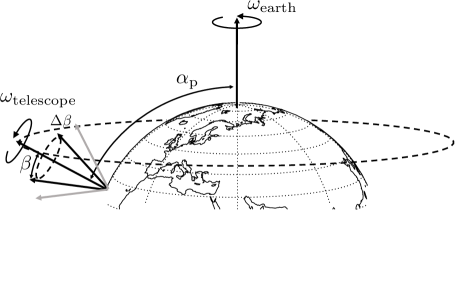
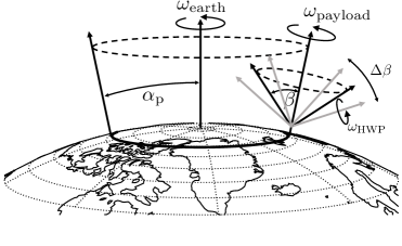
Figure 1: Observing strategy of the two instruments. Left: the LSPE-Strip telescope spins around the local zenith at an adjustable angle $\beta$. The spin velocity is set at 1 r.p.m. Right: the LSPE-SWIPE payload spin axis precesses around the North Pole, with precession angle equal to the co-latitude $\alpha_{\text{p}}$, with a velocity that is a combination of the daily Earth rotation with the natural wind drift. The telescope spins around the local zenith at an angle $\beta$ which can vary as $\Delta\beta$. The polarized signal is modulated by an Half-Wave Plate spinning at $\omega_{\text{HWP}}$. Numerical values are reported in table 13.

SWIPE is expected to have a fixed sky coverage of about $38\%$ of the Northern Sky, with the precise value depending on the choice of the launching station and effective trajectory. The sky fraction observed by LSPE-Strip can be adjusted by changing the telescope zenith angle [30], resulting in different sensitivity per sky pixel at the end of the survey. The final Strip strategy will be defined to trade-off the sky coverage with the noise per pixel distribution and to maximize the overlap between the sky regions observed by the two LSPE instruments.

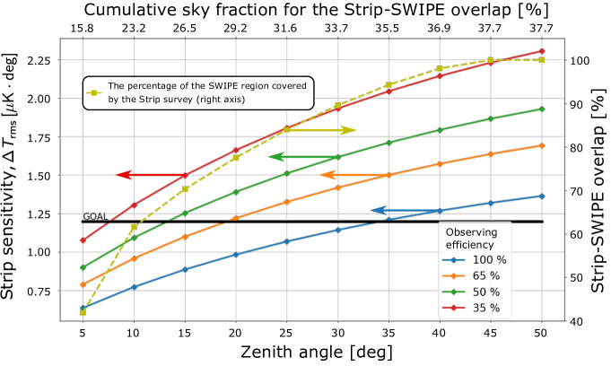
Figure 2: LSPE-Strip map sensitivity (left axis) as a function of the zenith angle (bottom axis) and observing efficiency (colors). The black line (left axis) represents the value of the map sensitivity as reported in table 1. The dashed gold line shows the Strip-SWIPE overlap percentage (right axis). The top axis reports the corresponding cumulative sky fraction. The arrows point, for each curve, towards the corresponding ordinate axis.

The baseline configuration of the Strip observation strategy assumes a constant zenith angle $\beta=$20\text{\thinspace}\mathrm{\SIUnitSymbolDegree}$$. Such configuration yields a map average noise $\sigma_{Q,U}=$102\text{\thinspace}\mathrm{\SIUnitSymbolMicro}\mathrm{K}\thinspace\mathrm{a}\mathrm{r}\mathrm{c}\mathrm{m}\mathrm{i}\mathrm{n}$$ at 43 GHz. Assuming two years of observation time, we can calculate the sensitivity with respect to this baseline value as a function of the zenith angle and of the usable fraction of time ( observing efficiency). This is shown in figure 2, together with the percentage of overlap, and the total sky fraction as a function of the zenith angle.

In the analysis reported in this paper, we assume a standard coverage for SWIPE, with a launch from Longyearbyen. In this case, the optimal overlap is obtained with a Strip zenith angle of $\beta=$35\text{\thinspace}\mathrm{\SIUnitSymbolDegree}$$, resulting in a full-frequency coverage over 37% of the sky, as shown in figure 3. The map noise is in this case $\sigma_{Q,U}=$130\text{\thinspace}\mathrm{\SIUnitSymbolMicro}\mathrm{K}\thinspace\mathrm{a}\mathrm{r}\mathrm{c}\mathrm{m}\mathrm{i}\mathrm{n}$$ at 43 GHz, with a wider coverage, providing the best trade-off for final results reported in sections 5. The two cases for Strip zenith angle $\beta=20$^∘ and $\beta=35$^∘ are listed in table1 as nominal and this-paper, respectively.

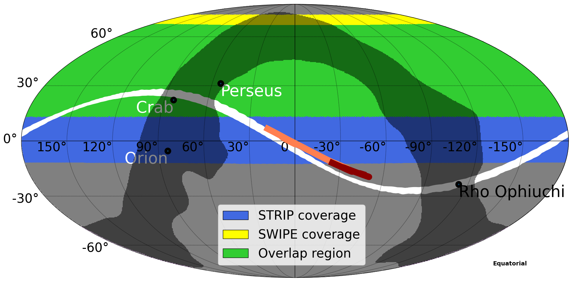
Figure 3: Map in Equatorial coordinates of the Strip-SWIPE coverage. The yellow area represents the SWIPE sky coverage; the blue area represents the Strip sky coverage, in the case of 35^∘zenith angle; the green area shows the overlap and the grey area represent a Galactic mask that covers 30% of the whole sky. The Stripcoverage ranges from -7 to 63^∘in latitude, and the SWIPE coverage from 13 to 77^∘. The map also shows the position of the Crab and Orion nebula, of the Perseus molecular cloud and the trajectories of Jupiter (orange), Saturn (dark red) and the Moon (white) from April 2021 to April 2023.

2.2 LSPE-Strip

LSPE-Strip is a coherent polarimeter array that will observe the microwave sky from the Teide Observatory in Tenerife in two frequency bands centred at $43\text{\thinspace}\mathrm{GHz}$ (Q-band, 49 receivers) and $95\text{\thinspace}\mathrm{GHz}$ (W-band, 6 receivers) through a dual-reflector crossed-Dragone telescope of $\sim$1.5\text{\thinspace}\mathrm{m}$$ projected aperture.

The Strip array uses coherent technology exploiting low noise high electron mobility transistor (HEMT) amplifiers, together with high-performance wave-guide components. The instrument is cooled to $20\text{\thinspace}\mathrm{K}$ by a two-stage Gifford-McMahon (GM) cooling system and integrated at the focal plane of the telescope that is able to rotate continuously in azimuth. The polarimeter’s design allows Strip to directly measure the Stokes $Q$ and $U$ parameters through a double- demodulation scheme that is explained in section 2.2.3. This design ensures excellent rejection of $1/f$ noise from amplifier gain fluctuations as well as of temperature-to-polarization leakage, without the need to introduce extra optical elements to modulate the polarized signal.

The main objective of Strip is to accurately measure Galactic synchrotron emission in the LSPE sky region in Q-band. Recent studies [31] show that the polarized synchrotron emission is significantly structured and characterized by non-trivial variations in its spectral index. Deep measurements at $43\text{\thinspace}\mathrm{GHz}$, complemented by lower frequency data, are crucial to constrain synchrotron contamination in the foreground minimum accounting for spectral index variations. Furthermore, achieving a resolution of $\sim 20$ arcmin will provide key information on the spatial properties of synchrotron foreground.

The W-band array, composed of 6 modules, will complement the Q-band data in monitoring the atmospheric load and fluctuations (mostly due to water vapor) during the Strip observations. Atmospheric effects in Q-band can be effectively monitored by measurements in W-band, where the water vapor component is significantly higher. Note anyway that at the Teide Observatory the atmospheric contamination of Q-band data is clearly dominated by O₂, which is stable spatially and with time. Yet the W-band channels will help to mitigate Q-band atmospheric fluctuations, expected to be of the order of $\sim 2$ K.

2.2.1 Observation site

Strip will be deployed at the Teide Observatory in Tenerife, at an altitude of $2400\text{\thinspace}\mathrm{m}$ above sea level, coordinates: $28\mathrm{°}⁤18\mathrm{\prime }⁤00\mathrm{″}$ N, $16\mathrm{°}⁤30\mathrm{\prime }⁤35\mathrm{″}$ W. The site provides excellent observing conditions and has been well-tested for astronomical observations for more than 30 years. The median precipitable water vapour is $3.5\text{\thinspace}\mathrm{mm}$, reaching values below $2\text{\thinspace}\mathrm{mm}$ during 30% of the time [32]. The inversion layer lies below the observatory for approximately 80% of the time.

The observatory has a long tradition in CMB research, including past experiments like the Tenerife radiometers [33], the IAC-Bartol [34], the JBO-IAC two-element interferometer [35], the COSMOSOMAS experiment [36] and the Very Small Array interferometer (VSA [37]). The Strip telescope will be installed inside an aluminium ground screen to limit interference and ground-spill. The telescope will be protected by a sliding roof that will cover the whole enclosure.

In addition to serving as low frequency monitor for LSPE, Strip also will complement two existing CMB experiments in Tenerife, QUIJOTE [38] and GroundBIRD [39], by observing in different frequency bands: 10–$40\text{\thinspace}\mathrm{GHz}$ for QUIJOTE, 40–$95\text{\thinspace}\mathrm{GHz}$ for Strip, and 145–$225\text{\thinspace}\mathrm{GHz}$ for GroundBIRD. All three Tenerife projects (QUIJOTE, LSPE-Strip and GroundBIRD) aim at measuring approximately the same area in the Northern sky and at degree scales, opening the possibility of future combined analyses, including useful redundancy for cross-checks of systematic effects. Strip measurements are currently scheduled to start during Summer 2022 and last two years.

The Strip telescope will scan the sky at a constant zenith angle, nominally 20^∘, with 1 r.p.m. azimuthal spin rate. This strategy will allow us to minimize atmospheric effects and to cover about 38% of the Northern sky, thus ensuring a large overlap with the SWIPE observations. After two years of operations with 50% observing efficiency we will reach a sensitivity of $\sim 102\text{\thinspace}\mathrm{\SIUnitSymbolMicro}\mathrm{K}_{CMB}\thinspace\mathrm{a}\mathrm{r}\mathrm{c}\mathrm{m}\mathrm{i}\mathrm{n}$ at $43\text{\thinspace}\mathrm{GHz}$ and $\sim 777\text{\thinspace}\mathrm{\SIUnitSymbolMicro}\mathrm{K}_{CMB}\thinspace\mathrm{a}\mathrm{r}\mathrm{c}\mathrm{m}\mathrm{i}\mathrm{n}$ at $95\text{\thinspace}\mathrm{GHz}$ (see section 2.1, table 1 and figure 2 for more details). The observing efficiency does not account for down time due to the Moon, glitches, Radio-Frequency Interference (RFI), or other unpredictable instrument-specific anomalies, thus moving our estimate somewhat on the optimistic side. A breakdown of our estimated data loss is given in the footnote of table 1.

2.2.2 Telescope and mount structure

The Strip telescope consists of two reflectors, a parabolic primary mirror and hyperbolic secondary mirror, arranged in a Dragonian cross-fed design, originally developed for the CLOVER experiment [40]. This configuration preserves polarization purity on the optical axis and gives low aberrations across a wide, flat focal plane. The projected diameter of the main reflector is $1.5\text{\thinspace}\mathrm{m}$ and the entire system has an equivalent focal length of $2700\text{\thinspace}\mathrm{mm}$, resulting in $\sim$ f/1.8.

The telescope is surrounded by a co-moving baffle made of aluminum plates coated by a millimetre-wave absorber, which reduces the contamination due to stray light. The optical assembly is installed on top of an alt-azimuth mount, which allows the rotation of the telescope around two perpendicular axes to change the azimuth and elevation angle. An integrated rotary joint will transmit power and data to the telescope and the instrument, and will allow a continuous spin as required by the scanning strategy. A general view of the Strip system is shown in figure 4.

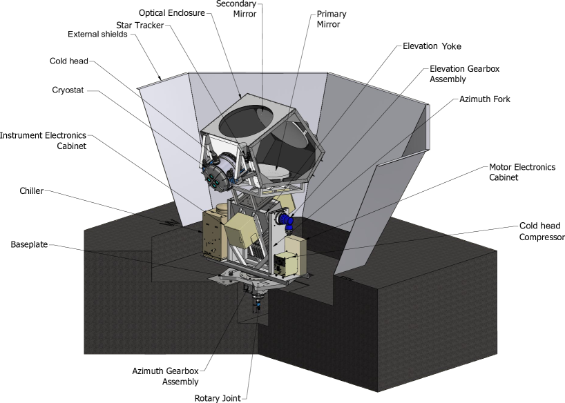
Figure 4: LSPE-Strip optical system overview. The mirrors are held inside a co-moving optical enclosure.

The telescope provides an angular resolution of $\sim$20^′ in the Q-band and $\sim$10^′ in the W-band. The feedhorn array is placed in the focal region, ensuring no obstruction of the field of view. All the modules are optimally oriented according to the shape of the focal surface, with illumination centred on the primary mirror. The two mirrors determine the main beam shapes of the Strip detectors, while the shielding structures affect the near and far sidelobes [41].

Optical performance.

We have modeled the optical assembly with the GRASP software and the model includes the nominal reflectors, the focal plane unit, the IR filters, and the shielding structures. The model is also able to reproduce the dual circular polarization antenna-feed system [42].

We have simulated the main beam radiation patterns using the Physical Optics (PO) method, which is needed to correctly model the detector patterns in the far field. Given the off-axis configuration, the main beams are characterized by several parameters, such as the angular resolution, the ellipticity, the main beam directivity, and the cross-polar discrimination factor (XPD).

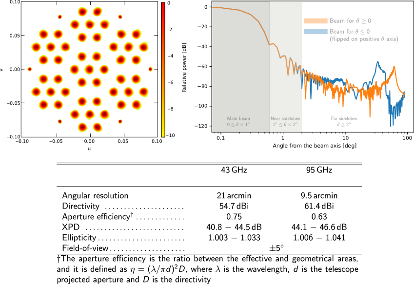
Figure 5: Left: footprint of the LSPE-Strip main beams in the $(u,v)$ plane (large beams, 43 GHz, small beams, 95 GHz). Right: beam cut for $\phi=0$ of the central horn. We have flipped the beam section for $\theta<0$ on the positive axis to better highlight the asymmetries. The $(u,v)$ variables are defined as $u=\sin(\theta)\cos(\phi)$, $v=\sin(\theta)\sin(\phi)$, where $(\theta,\phi)$ are standard spherical coordinates, with the center of the telescope pointing towards $\theta=0$. The inset table reports the averaged main optical parameters.

Sidelobes have been computed using the Multi-Reflector Geometrical Theory of Diffraction (MrGTD). While less accurate than PO, this ray-tracing technique is much more efficient and it is able to predict the full-sky radiation pattern of complex optical systems. The $4\pi$ radiation patterns show unevenly distributed features that are due to multiple reflections inside the shielding structure and rays entering the feedhorns without any interaction with the reflectors. Each contribution has been analyzed separately and then combined in an integrated model beam. We find that the level of sidelobes at angles larger than $1\text{\thinspace}\mathrm{\SIUnitSymbolDegree}$ is less than $-55\text{\thinspace}\mathrm{d}\mathrm{B}$ at $43\text{\thinspace}\mathrm{GHz}$ and less than $-65\text{\thinspace}\mathrm{d}\mathrm{B}$ at $95\text{\thinspace}\mathrm{GHz}$.

In the top-left panel of figure 5 we show the footprint of the Strip main beams in the $(u,v)$ plane. We can see the 49 Q-band beams grouped in seven hexagonal structures of seven beams each and the six outer W-band beams. In the top-right panel of the same figure we show a cut corresponding to $\phi=0$ of the central beam. We have flipped the beam section for $\theta<0$ on the positive axis to better highlight the asymmetries. The bottom inset table displays the average main optical parameters.

2.2.3 Instrument and cryogenics

The Strip focal plane array of corrugated feedhorns is placed inside the dewar surrounded by a radiative shield cooled to $80\text{\thinspace}\mathrm{K}$ by the cooler first stage (see the left panel of figure 6).

Copper thermal straps connect the focal plane and the cooler cold head allowing the polarimeter chain to be cooled down to $20\text{\thinspace}\mathrm{K}$. The cryostat window is an ultra-high molecular weight polyethylene (UHMWPE) window with a diameter of 586 mm and a thickness of 56.34 mm. We stop the IR radiation from the $300\text{\thinspace}\mathrm{K}$ environment with 13 polytetrafluoroethylene (PTFE) filters with anti-reflection coating at $150\text{\thinspace}\mathrm{K}$. We have one filter for each horn at $95\text{\thinspace}\mathrm{GHz}$ (diameter 52 mm and thickness 23 mm) and one filter for each 7-horns module at $43\text{\thinspace}\mathrm{GHz}$ (diameter 170 mm and thickness 23 mm). The filters are attached to the 100 K thermal shield in front of the 20 K feedhorn array.

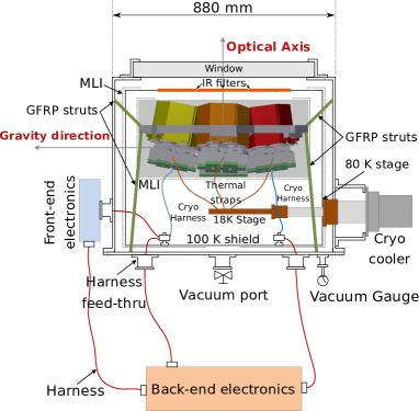
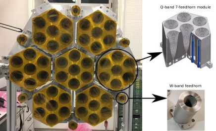
Figure 6: Left: schematic drawing of the Strip instrument. The focal plane array is inside the cryostat surrounded by the $80\text{\thinspace}\mathrm{K}$ shield and thermally connected to the cooler cold head. Note that this drawing does not include the W-band horns that are visible in the real picture on the right. Right: the complete Strip focal plane array with 49 feedhorns in Q band and 6 feedhorns in W band. We also show a cutaway of one Q-band module (top) and the detailed view of one of the six W-band feedhorns (bottom).

The detector assembly is based on coherent polarimeters connected to an optical chain constituted of corrugated feedhorns, each coupled to a polarizer-orthomode transducer (OMT) system at 43 GHz and to a septum polarizer at 95 GHz [43].

Feedhorns.

The feedhorns are designed implementing a dual profile to obtain an optimal illumination of the secondary with a limited feed size, and are manufactured in aluminum using the platelet technique [44]. The right panel of figure 6 shows a picture of the entire Strip focal plane, with the 49 Q-band feedhorns arranged in 7-unit modules surrounded by the six W-band feedhorns. A cutaway of one of the Q-band modules and a detailed view of one of the W-band feedhorns are also presented. In the cutaway it is possible to appreciate the platelet structure of the module and the tightening screws that allowed to assemble the horns without the need of bonding material or thermal brazing. In figure 7 we show the corrugation profile of the Strip feedhorns in both frequency bands and a summary table of the main parameters.

Figure 7: Corrugation profile of Q- and W-band Strip feedhorns. The inset table summarizes the main feed parameters.

Polarizers and OMTs.

Each feedhorn is connected to a polarizer system that converts the two orthogonal components of the electric field, $(E_{x},E_{y})$ into right- and left-circular polarization components, $\left[(E_{x}+i\thinspace E_{y})/\sqrt{2},(E_{x}-i\thinspace E_{y})/\sqrt{2}\right]$, which propagate through the polarimeter module. This conversion is obtained differently in Q- and W-band.

In Q-band we convert linear to circular polarization using a groove polarizer [45] connected to a platelet OMT [46]. In figure 8 we show the complete set of Q-band polarizers (left panel) and OMTs (right panel) implemented in the Strip focal plane. This solution allowed us to obtain a very good measured performance in terms of transmission ($\gtrsim$-0.5\text{\thinspace}\mathrm{d}\mathrm{B}$$), reflection ($<$-25\text{\thinspace}\mathrm{d}\mathrm{B}$$) and cross-talk ($\sim$-40\text{\thinspace}\mathrm{d}\mathrm{B}$$).

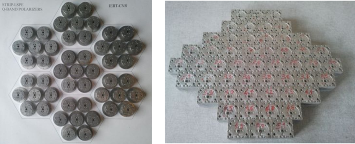
Figure 8: Left: the 49 Strip Q-band polarizers arranged according the 7-module feedhorn footprint. Right: the 49 Strip Q-band platelet OMTs

Each W-band channel incorporates a septum polarizer characterized by a reflection of $<$-20\text{\thinspace}\mathrm{d}\mathrm{B}$$ and a leakage of intensity to polarization of the order of $\sim-$13\text{\thinspace}\mathrm{d}\mathrm{B}$$. The detailed design and performance of these components, originally used by the QUIET $95\text{\thinspace}\mathrm{GHz}$ instrument [47], can be found in [48].

Polarimeters.

The Strip Q-band channel uses a combination of the original 19 QUIET Q-band modules [49] and additional 30 units that were developed according to the same design. The W-band channel uses 6 QUIET polarimeters selected among those with the best performance. The diagram in figure 9 shows the operation principle. If two circularly polarized signals propagate through a symmetric $180^{\circ}$ hybrid, the power detected at its output is a combination of $I$ and $Q$ Stokes parameters, with $Q$ having opposite signs at the two detectors. The detected power at the output of a second, 90^∘ hybrid coupler yields a combination of $I$ and $U$, with $U$ appearing with opposite signs. The design takes full advantage of the coherent nature of the signal, implementing a double demodulation scheme to minimize residual systematic effects. This strategy allows Strip to recover both $Q$ and $U$ from a single measurement, after combining the two linearly polarized components of the input field, $E_{x}$ and $E_{y}$, into left and right circular polarization components.

Figure 9: The Strip polarimeter’s operation principle. The figure also shows the main mathematical relationships among the detected power at the four diodes, $P_{Q_{1,2}},P_{U_{1,2}}$, the Stokes parameters defined in the polarizer reference frame, $I,Q,U$ and the polarimeter noise temperature, $T_{\mathrm{noise}}$.

Ahead of the first hybrid, two multi-stage Indium Phosphide (InP) HEMT amplifiers provide about $50\text{\thinspace}\mathrm{d}\mathrm{B}$ amplification while two phase switches shift the signal phase between 0^∘ and 180^∘, and allow demodulation.

There are two different kinds of demodulation. A fast ($\sim$4\text{\thinspace}\mathrm{kHz}$$) demodulation, provided by one of the two phase switches that flips the signs of $Q$ and $U$ at each of the four diodes (see figure 9), removes effectively the effect of amplifier gain fluctuations. A slow ($50\text{\thinspace}\mathrm{H}\mathrm{z}$) demodulation, provided by the second switch that flips the sign between detector pairs, removes any $I\rightarrow Q,U$ leakage arising from asymmetries in the phase switches attenuation. Note that it is irrelevant which of the two phase switches is “fast” and which one is “slow”.

The correlation units are packaged into square brass modules about $1\text{\thinspace}\mathrm{c}\mathrm{m}$ thick and with a footprint of $\sim 5\times$5\text{\thinspace}\mathrm{c}\mathrm{m}^{2}$$ in Q-band and $\sim 2.5\times$2.5\text{\thinspace}\mathrm{c}\mathrm{m}^{2}$$ in W-band. Each complete polarimetric chain from the feed to the detectors will be cooled down to $20\text{\thinspace}\mathrm{K}$ by the Strip cryogenic system.

Electronics.

The Strip electronics provides the full biasing and acquisition of the 55 polarimeters on the focal plane. It consists of 7 pairs of boards that drive and acquire data from 8 polarimeters each. Each pair contains one bias board and one Data AcQuisition and logic board (DAQ), shown in the left panel of figure 10.

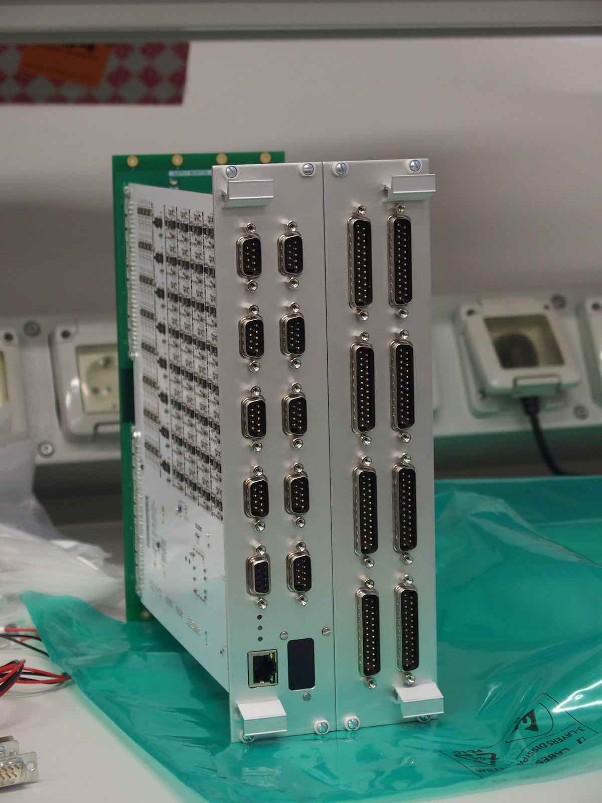
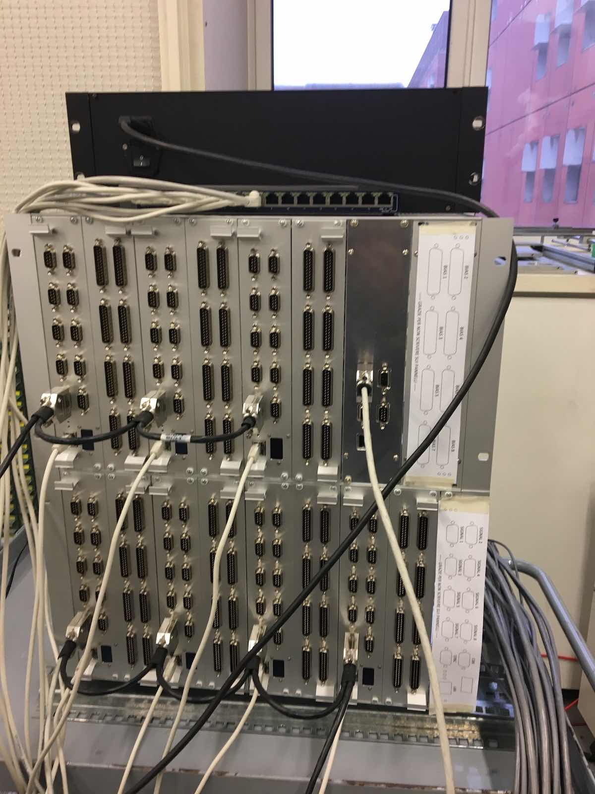
Figure 10: Left: one of the 7 modules of Strip electronics composed of one bias board on the right and one data acquisition and logic board (DAQ). Both are connected to a back-plane (in green) for stabilized power supply and data exchange between the two boards. Right: the two 6U $19\text{\thinspace}\mathrm{i}\mathrm{n}\mathrm{c}\mathrm{h}\mathrm{e}\mathrm{s}$ racks containing the Strip electronics during the final tests.

The bias voltages are set and monitored by the bias board that controls the HEMT low noise amplifiers (LNAs) and phase switches. All the phase switches of all the 7 board pairs are synchronized by a master-clock signal generated and distributed by the GPS and Master-Clock board through a dedicated daisy-chain cable. The bias board can operate the LNAs in open- or closed-loop. In open loop the drain and gate voltages of every transistor are set according to an optimum configuration found during the unit- and system-level tests, and the drain current is simply monitored through the bias house-keeping. In this case bias voltages are susceptible to variations of the focal plane temperature. In closed loop we set the drain voltages and currents, and a completely analogue loop adjusts the gate voltages to keep the desired currents. The closed loop mode is useful in case of excessive temperature instability and its use will be particularly important during the commissioning phase.

The DAQ boards have two functions: they interact with the main computer via telemetry-telecommands and acquire the data generated by the four detectors of each polarimeter. Each board controls 8 polarimeters and receives and stores their bias settings from the main computer via Ethernet network. In this way, the operations can autonomously restart in case of communication loss after a black-out. The bias settings are then passed to the bias board. Each DAQ board acquires data from 32 detectors at a rate of $1\text{\thinspace}\mathrm{M}\mathrm{H}\mathrm{z}$, demodulates the scientific data at the fast phase switch rate ($4\text{\thinspace}\mathrm{k}\mathrm{H}\mathrm{z}$), prepares the data packets with scientific signals, housekeeping data and time tags obtained from the GPS/master clock and sends the data via Ethernet to the main computer for storage.

A field programmable gate array (FPGA) on the DAQ board carries out the mathematical operations as well as the digital-to-analog (DAC) and analog-to-digital (ADC) conversions, while a microcontroller handles the communication with the main computer, decodes and routes the commands towards the FPGA and assembles the data packets. The data stream produced by the seven DAQ boards is $\sim$2\text{\thinspace}\mathrm{M}\mathrm{b}\mathrm{/}\mathrm{s}$$, well below the maximum Ethernet capability.

The full electronics occupies two 6U $19\text{\thinspace}\mathrm{i}\mathrm{n}\mathrm{c}\mathrm{h}\mathrm{e}\mathrm{s}$ racks (right panel of figure 10) that will be positioned close to the dewar and protected by two IP55 grade cabinets.

2.3 LSPE-SWIPE

LSPE-SWIPE (Short-Wavelength Instrument for the Polarization Explorer) is a mm-wave polarimeter operated onboard a stratospheric balloon. The general idea of SWIPE is to use a cryogenic rotating Half-Wave Plate to modulate the incoming polarized radiation and to maximize the sensitivity to CMB polarization at large scales using a very wide focal plane populated with multi-moded bolometers.

The spectral coverage of SWIPE has been optimized to be very sensitive to CMB polarization with one broad-band channel matching the peak of CMB brightness ($145\text{\thinspace}\mathrm{G}\mathrm{H}\mathrm{z}$, 30% bandwidth), and to be able to monitor and separate the signals from interstellar dust (the main polarized foreground at this frequency) by means of two ancillary, narrower channels at 210 and $240\text{\thinspace}\mathrm{G}\mathrm{H}\mathrm{z}$. These are dedicated to measuring the slope of the specific brightness of interstellar dust.

The focal planes of SWIPE are large enough that a total of 8800 modes of the incoming radiation are collected by the multi-moded 326 detectors, thus boosting the sensitivity of the polarimeter to unprecedented levels for such a comparatively low number of detectors. The detectors arrays are cooled to $0.3\text{\thinspace}\mathrm{K}$ by a large wet cryostat, which also cools the polarization modulator and the entire telescope.

The cryostat is mounted in a frame, the gondola, providing accommodation for an attitude control system, the power system and electronics. The gondola interfaces to the flight train of the stratospheric balloon through an azimuth pivot allowing for azimuth spin and/or scan. A general view of the SWIPE instrument is shown in figure 11.

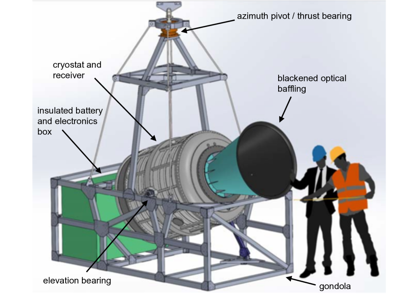
Figure 11: LSPE-SWIPE overview. The instrument is contained in a large liquid Helium cryostat, which also contains the optical elements, including the HWP based Stokes polarimeter. The on-board electronics and the Lithium batteries based power system are contained in an Aerogel insulated box, to optimize thermal balance.

LSPE-SWIPE measurements are currently scheduled for Winter 2022/23.

2.3.1 Winter polar balloon flight

LSPE-SWIPE is designed to fly on a stratospheric long-duration balloon in the arctic winter. Stratospheric balloon altitudes (about $35\text{\thinspace}\mathrm{k}\mathrm{m}$ above sea level) are needed to avoid most of the atmospheric emission, which is relevant at $145\text{\thinspace}\mathrm{G}\mathrm{H}\mathrm{z}$ and very important at higher frequencies. A winter launch guarantees the possibility to exploit the absence of the Sun and cover a large fraction of the sky by spinning the full payload, allowing efficient exploration of the CMB polarization anisotropy at large angular scales. It also ensures higher stability of the observing conditions, due both to the thermal stability of the instrument and to the lowest residual turbulence in the atmosphere.

The instrument is designed for a 15-day long flight. This long duration is needed to reach the sensitivity that matches the scientific goal of the LSPE experiment. Options for launching in the polar night are at the moment only possible from the Northern Hemisphere, due to the logistics difficulties related to the access to Antarctic regions during austral winter. In particular, two possible launching stations are Longyearbyen, in the Svalbard islands (Norway), with a latitude above 78.2^∘N, and Kiruna (Sweden) at a latitude of 67.8^∘N. Several launches have been performed from Longyearbyen, with different balloon and payload sizes, both in Summer and in Winter over the last few years. Kiruna offers an established alternative, although at lower latitudes. Stratospheric balloon flights are organized by the Swedish Space Corporation in the Esrange Space Center.

In order to assess the feasibility of winter polar northern hemisphere flights, we have developed a trajectory simulator, based on the publicly available data from The Research Data Archive (RDA), managed by the Data Support Section (DSS) of the Computational and Information Systems Laboratory (CISL) at National Center for Atmospheric Research (NCAR). With these data is possible: (1) to simulate balloon trajectories in the past years, for a statistical analysis of flight opportunities; (2) to predict trajectory in the near future, based on a stratospheric wind model, with a prediction of 225 hours in the future; and (3) to compare historical predictions and historical data, to assess prediction reliability.

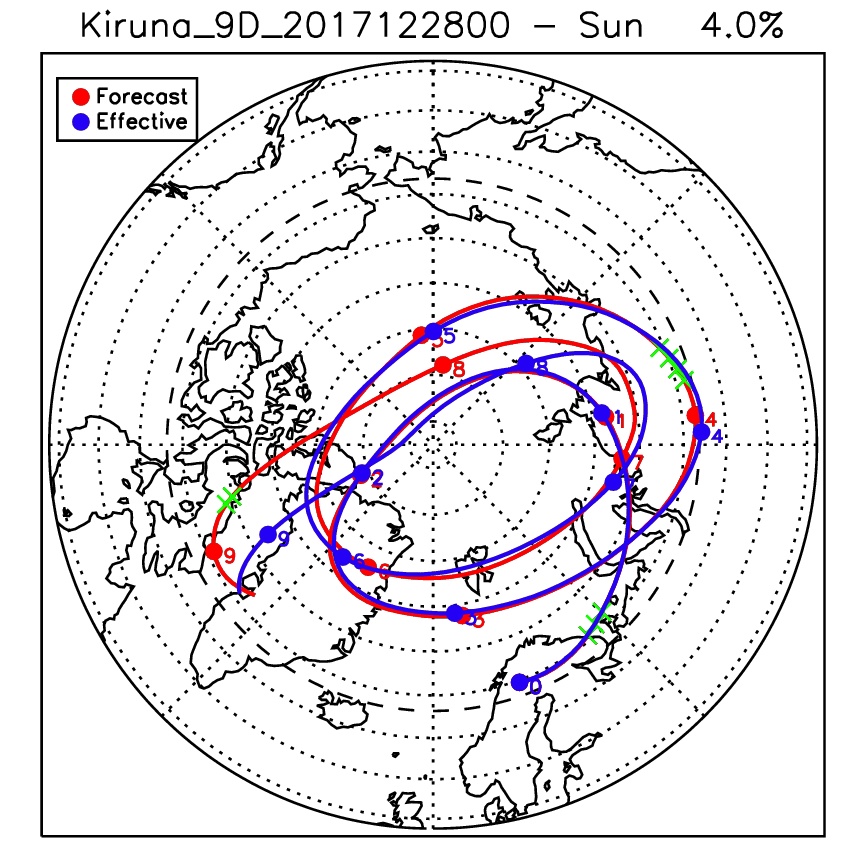
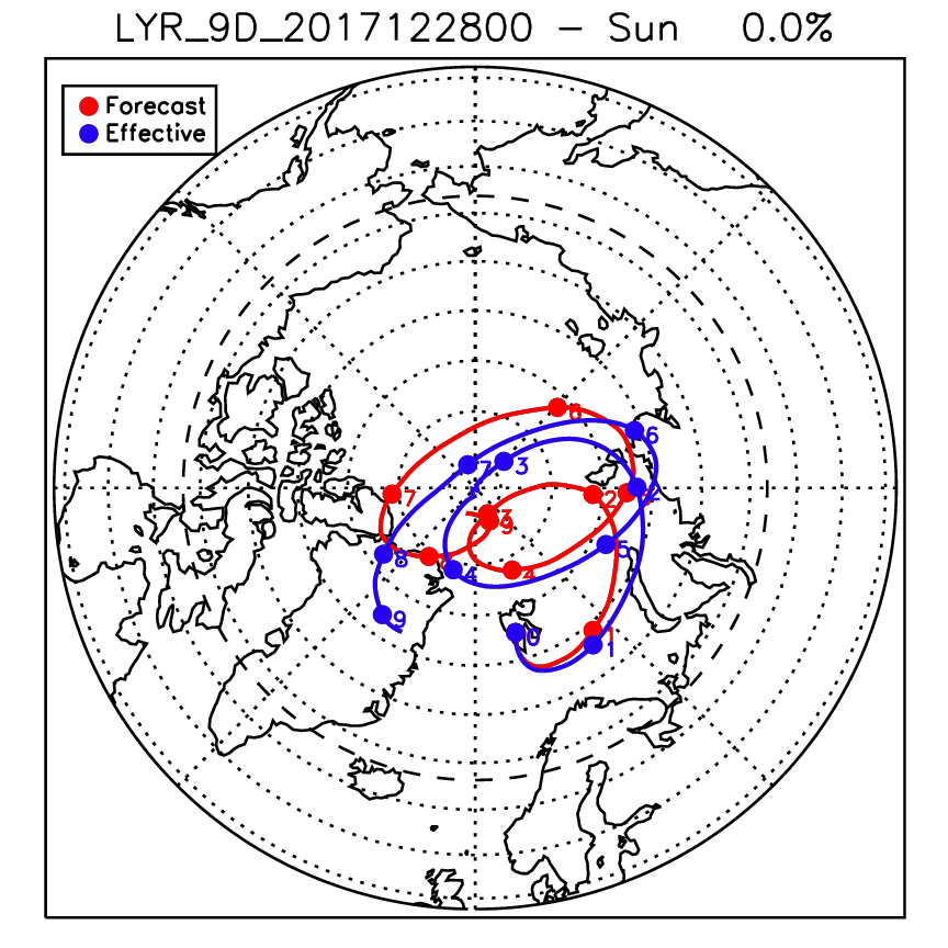
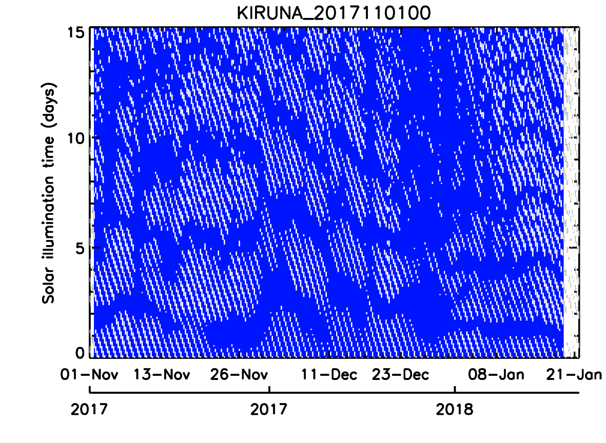
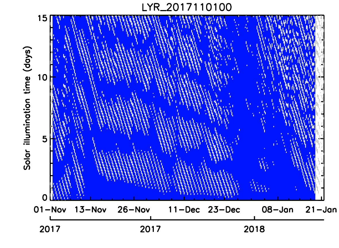
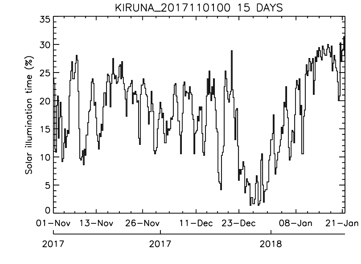
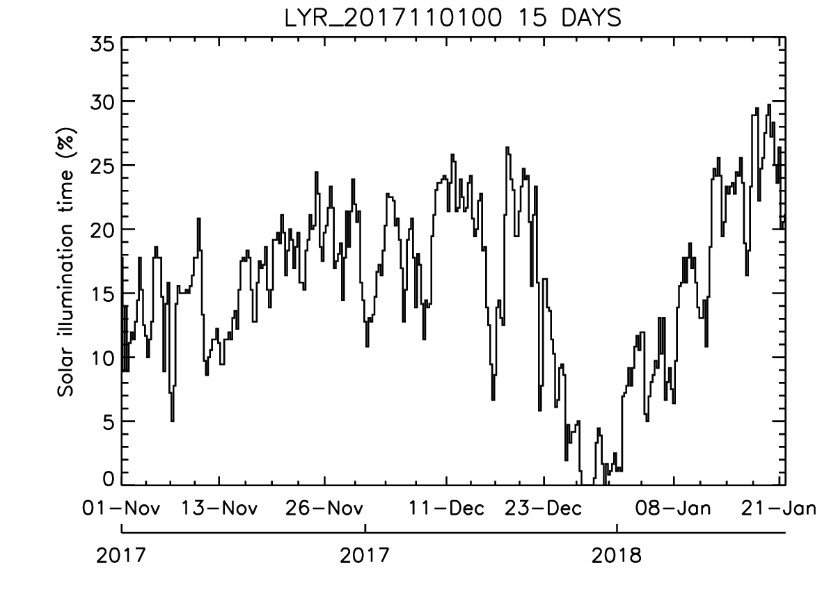
Figure 12: Winter polar northern hemisphere trajectories and statistical analysis. Left column plots are for a launch from Kiruna and right plots from Longyearbyen. Top: in red a simulated trajectory based on historical forecast, for 9 days after a launch on December 28, 2017; in blue the simulated trajectory based on historical data, for the same launch day. Dots represent 24 hours steps. The green dot indicates hours with solar illumination on the payload (Sun higher than $-$4\text{\thinspace}{}^{\circ}$$ above the horizon). The trajectory based on wind prediction is very well reproduced by the trajectory based on real wind data. Center: the panels show an analysis of full winter 2017/18. The abscissa axes indicate the launch date. The ordinate axes indicate the days of flight. For every hour of flight, a blue dot represents an hour in the dark, while a white dot represents an hour with solar illumination. A fully blue vertical area indicates a launch day with full flight in the dark. Bottom: the plots report the fraction of time with solar illumination given a launch day.

Figure 12 illustrates a snapshot of trajectories’ statistical analysis, that will be included in a separate paper. The simulation tool has also been validated by comparison of predictions with real trajectories, for Summer and Winter flights. The payload recovery is essential in the case of LSPE-SWIPE, due to the detectors’ data-rate higher than the possible telemetry rate. From the top panels of figure 12 it is clear that the typical winter trajectory is followed with a much higher speed with respect to summer trajectories. For this reason, the probability to have the payload stalled over the ocean is low, increasing the recovery chances, with unpredictable difference between the two considered launch sites.

Such a long duration flight in the winter, while being appealing from the scientific point of view, is very demanding in terms of power system and thermal balance. A series of technological test flights has been carried out over the years, as reported in [50, 51, 52, 53, 54]. All the LSPE-SWIPE parts are designed to cope with temperatures as low as $-90\text{\thinspace}\mathrm{\SIUnitSymbolCelsius}$, except the battery pack and part of the electronics, which are contained in a thermally insulated box.

2.3.2 Power supply

For a long-duration night-time flight, a relatively cheap, consolidated, high energy-density power-supply solution is based on lithium batteries. The total power budget of the SWIPE instrument is $\sim$370\text{\thinspace}\mathrm{W}$$, and the energy necessary for the entire mission is $\sim$0.48\text{\thinspace}\mathrm{G}\mathrm{J}$$. This is stored in a stack of $\sim$ 3500 cells (each $14\text{\thinspace}\mathrm{A}\mathrm{h}$ @ $3.3\text{\thinspace}\mathrm{V}$). Due to the low internal resistance of these cells, and the fact that their capacity decreases at low temperatures, it is necessary to keep the cells warm (at a temperature $>$0\text{\thinspace}\mathrm{\SIUnitSymbolCelsius}$$) during the flight. This is obtained by hosting the batteries in the same box hosting the electronics of the experiment, and in good thermal contact. The box is insulated from the cold external environment by a blanket made of three layers of metal reflective foil separated by two thick ($\sim$2.5\text{\thinspace}\mathrm{c}\mathrm{m}$$) layers of aerogel. According to the thermal model, with $200\text{\thinspace}\mathrm{W}$ of power dissipated in the electronics inside the box, and an external temperature of $200\text{\thinspace}\mathrm{K}$, the internal temperature is maintained at $280\text{\thinspace}\mathrm{K}$. A prototype of this power and thermal insulation system was flown in a winter arctic balloon in December 2017 [54], and further tests are planned for the future.

2.3.3 Gondola and pointing system

The gondola is a simple riveted frame of aluminum beams, hosting all the components of the payload and of the flight system, and structurally optimized to withstand an acceleration of 10 g (${\rm g}={\rm gravitational}$ acceleration) at the opening of the parachute after the flight termination. The telescope attitude is controlled by the attitude control system (ACS). Its main purpose is to spin in azimuth the entire gondola. The azimuth pivot separates the payload from the flight chain, and is based on thrust bearings and a torque motor. The motor torques directly against the flight chain, to obtain an azimuth spin rate up to $10\text{\thinspace}{}^{\circ}\mathrm{/}\mathrm{s}$, much faster than the nominal rate of $0.7\text{\thinspace}{}^{\circ}\mathrm{/}\mathrm{s}$ .

Mechanically and electrically, the system is very similar to the ones used in ARGO [55], BOOMERanG [56, 57], Archeops [58], OLIMPO [59, 60, 61], and described in detail in [62, 63, 64]. Given the measured friction of the thrust ball bearing, we expect to use up to $\sim$70\text{\thinspace}\mathrm{W}$$ to rotate the $\sim$2000\text{\thinspace}\mathrm{k}\mathrm{g}$$ payload at the $10\text{\thinspace}{}^{\circ}\mathrm{/}\mathrm{s}$ scan speed. The azimuth speed is sensed by a laser-gyroscope, the signal of which is compared to the desired spin rate, in a feedback loop controlling the current in the torque motor. The elevation of the boresight can be changed by tilting the entire cryostat, using a geared DC motor driving a linear actuator with linear recirculating ball bearing. The pointing reconstruction is based on a high altitude GPS receiver to obtain geographical coordinates and on two orthogonal fast star sensors [65], the same successfully used for the Archeops flight [66], for the celestial coordinates of the boresight. The system allows for pointing reconstruction with $\sim$ arcmin accuracy.

2.3.4 Cryostat

SWIPE makes use of a custom-designed main cryostat with a bath of $250\text{\thinspace}\mathrm{l}\mathrm{i}\mathrm{t}\mathrm{e}\mathrm{r}\mathrm{s}$ of superfluid helium, connected to the external low-pressure environment to operate at $1.6\text{\thinspace}\mathrm{K}$. The cryostat shell, the internal shields and the LHe tank are all made of aluminum alloys, to reduce their mass, as developed for the cryostats used in the ARGO [67], BOOMERanG [68], PILOT [69] and OLIMPO [70] balloon-borne instruments. Two vapor-cooled intermediate shields, separated by super-insulation blankets, are used to minimize the radiative heat load on the LHe bath. The main cryostat provides the base temperature to cool down the polarization modulator and the optical system, and to operate a ³He evaporator [71]. The latter cools down to $0.3\text{\thinspace}\mathrm{K}$ the two focal plane arrays, as required to operate the SWIPE bolometric detectors. The hold time forecast for the LHe in the main cryostat is $\sim$20\text{\thinspace}\mathrm{d}\mathrm{a}\mathrm{y}\mathrm{s}$$, while the ³He refrigerator has a hold time of $\sim$7\text{\thinspace}\mathrm{d}\mathrm{a}\mathrm{y}\mathrm{s}$$, and can be recycled in flight. In order to minimize the radiative load on the detectors, the 600 mm diameter window has been designed in a similar way as the one used by the EBEX group [72], and, less recently, in [73] and in [74]. In practice, a thick UHMWPE [75] window used for laboratory tests is removed at float, leaving only a very thin ($\ll\lambda$) Mylar window to withstand the small pressure difference between the cryostat vacuum and the stratospheric pressure. The thick window also implements a highly reflective filter to operate the receiver on the ground under radiative loadings representative of the stratospheric environment. Just before the termination of the flight, the motor unit is remotely operated again to put the thick window back in place for a relatively safe receiver landing.

2.3.5 Optical system

The optical system of LSPE-SWIPE (figure 13) consists in a single-lens, $490\text{\thinspace}\mathrm{m}\mathrm{m}$ aperture refractor telescope, focusing incoming radiation on two large curved focal planes, split by a large wire grid (WG) polarizer. Polarization modulation is obtained by a cryogenic $500\text{\thinspace}\mathrm{m}\mathrm{m}$ wide rotating Half-Wave Plate which is placed skywards of the lens, below the window and the warm thermal filters. The large plano-convex lens, attached to the 1.6 K stage of the cryostat, is made of High Density Polyethylene (HDPE), ensuring a very good transmittance across the bands and limited dielectric losses at high frequencies. Typical dielectric properties of HDPE are a refractive index $n=1.52$ and a loss tangent of $\sim 5\times 10^{-4}$. The baseline optical design is based on these numbers, but further optimization will be performed after characterizing at low temperatures a sample from the same batch that will be actually used to build the lens. A layer of anti-reflection coating based on porous PTFE will be deployed on the lens surfaces in order to minimize reflection losses. Full-aperture IR-blocking filters are arranged on each available thermal sink along the path from the window to the lens. Two more such filters are placed at 1.6 K on the path to the focal plane directly below the lens. These are designed to cut most of the radiation emitted out of band by the HWP, its rotation mechanism and the lens itself. The final stage of spectral selection and band refinement is performed directly on the $300$ mK stage, where small-aperture packs of bandpass and low-pass filters are mounted on the mouths of the pixel horns. Each focal plane is populated with 163 multi-moded horn antennas, each feeding a spider-web Transition Edge Sensor (TES) bolometer.

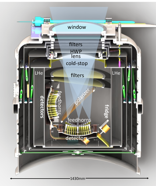
Figure 13: LSPE-SWIPE cryostat and optical system. Radiation enters from the top window, passes across filters, HWP, lens, cold-stop, and other filters. It then is split by the large wire grid and collected in the two curved focal planes.

The configuration fulfills our requirements with a low cross-polarization ($<1\%$) and a controlled instrumental polarization (including an absorption component $<0.04\%$ and an extremely low, and stable, emitted component by the use of a cold telescope). These values are reached at the edge of the corrected focal plane for all the 3 bands and they are negligible on axis. Besides the 490 mm diameter lens the system adopts a 460 mm diameter cold aperture stop close to the lens (corresponding to an entrance pupil of 487 mm diameter) and located on the opposite side of the lens with respect to the polarization modulator. The FOV, 20^∘ wide, is split by a $500\text{\thinspace}\mathrm{m}\mathrm{m}$ diameter 45^∘ tilted wire grid in 2 curved focal planes (CFP_T and _R) $300\text{\thinspace}\mathrm{m}\mathrm{m}$ in diameter, with a resulting focal ratio of 1.75. The full optical system is kept at cryogenic temperature in the LSPE-SWIPE cryostat, in order to minimize its radiative loading on the detectors and to mitigate the signals due to the thermal emittance of the rotating HWP.

The design rationale of the SWIPE focal plane is based on a trade-off between the sensitivity and the angular resolution of the instrument, by trying to maximize the power collection efficiency of each detector at the selected resolution. This requirement clearly sets a constraint for the size of the focal plane region which must be covered by a single detector, and ultimately determines the collection area of an individual sensitive element of the receiver. In order to further improve the pixel efficiency, detectors are coupled to their corresponding focal plane pixel through multi-moded feedhorns [76]: large-aperture smooth-walled conical horn antennas feed the detectors by matching freespace radiation to multi-moded circular waveguides located at the horn throat. The waveguides select a frequency-dependent number of propagating modes (i.e. solutions to the propagation problem as constrained by the boundary conditions set by the waveguide geometry) so that for any given geometrical aperture of the horn, higher-order waves contribute in shaping the beam response of the horns. This results in a more flat-top (and broader) beam profile, with an overall higher illumination efficiency of the system pupil, and therefore a higher pixel throughput within the portion of its field of view which is used to collect radiation from the sky.

Under the assumption that radiation detection is based on purely incoherent processes on the detector absorber, the phase relation among the coupled modes is not relevant to determine the coupling efficiency. Therefore, electromagnetic modeling of the horn-waveguide assembly can be easily performed by solving one reverse-propagation problem per each of the coupled modes selected by the waveguide. A far-field calculation of the field solution at the horn aperture then yields the individual contribution of each mode to the horn response, and the full multi-moded response is then computed as a power summation over the coupled modes. This operation has been performed through the Ansys HFSS software, and the calculated beam profile for the SWIPE horns is shown in figure 14. Here the contributions from the individual modes have been evenly weighted, as expected under energy equipartition conditions, and confirmed by numerical simulation of the absorber/cavity sub-system (see section 2.3.7). A measurement of the feed angular response is reported in [77].

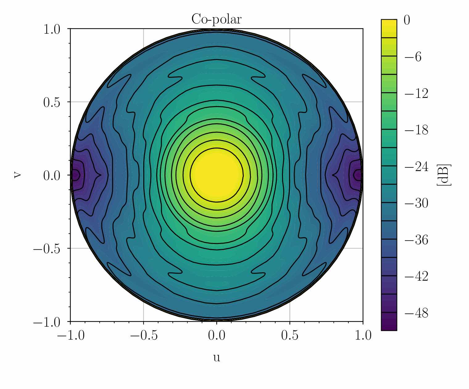
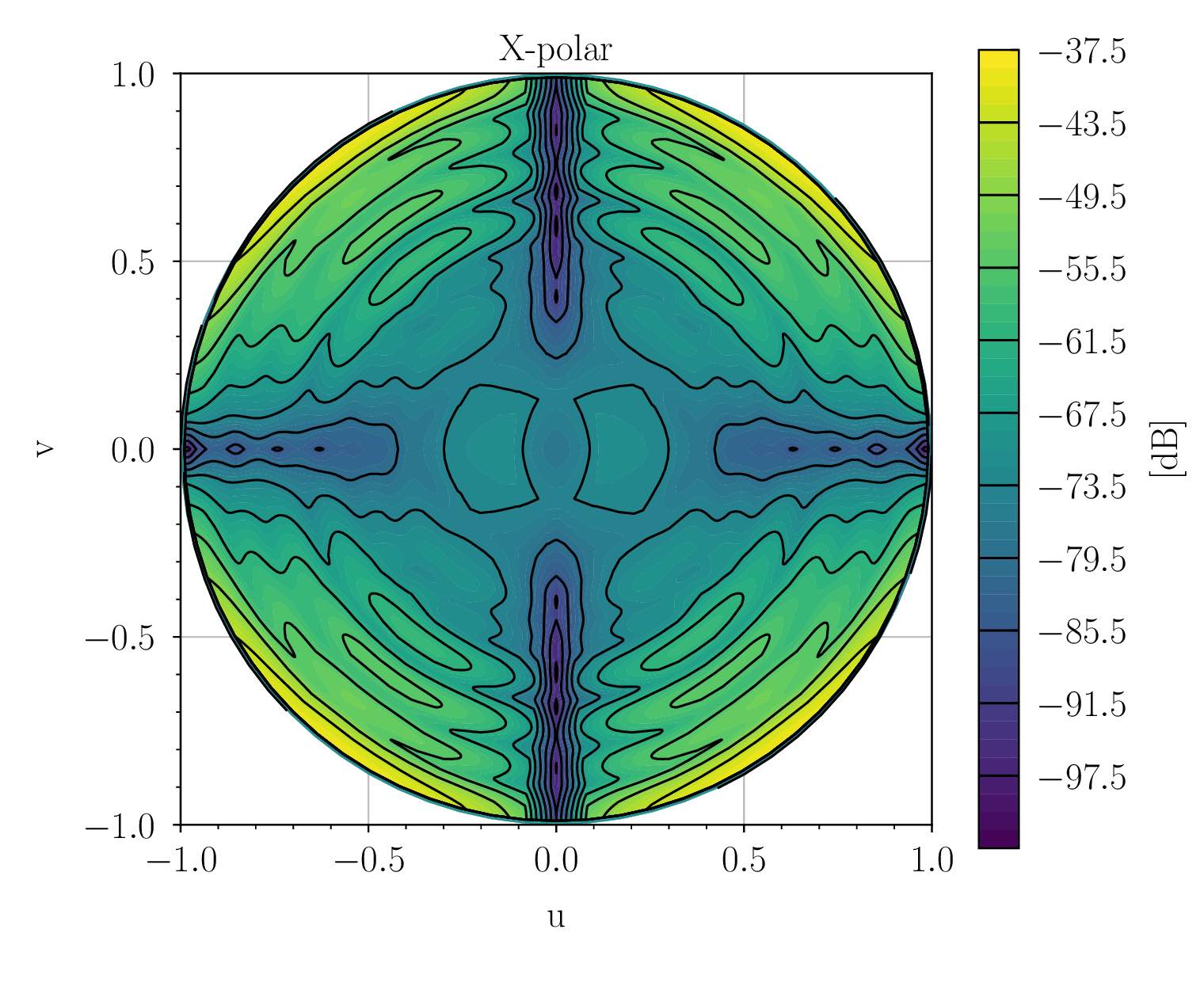
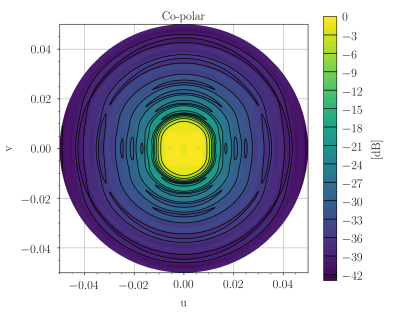
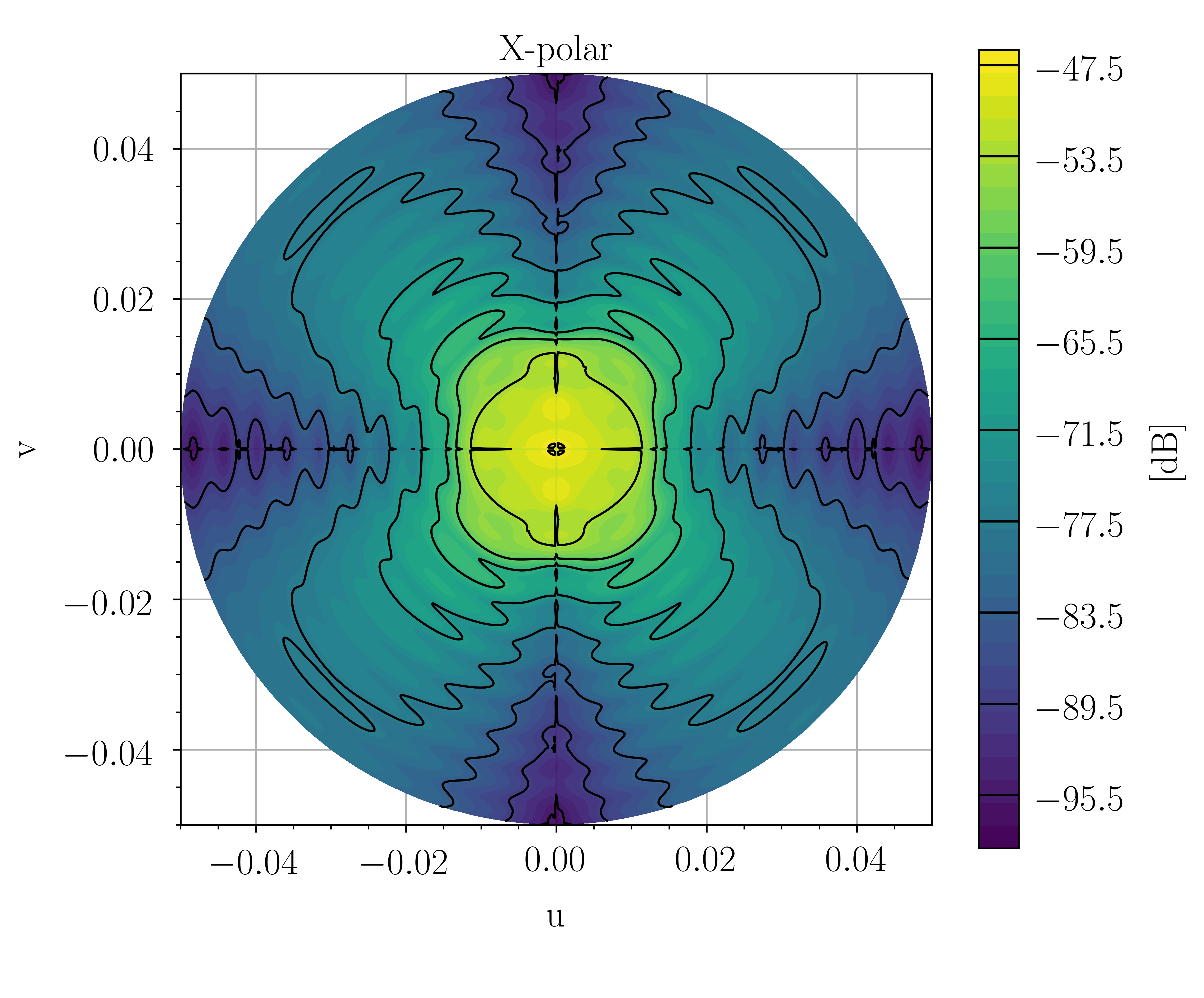
Figure 14: Top panels: simulated beam response of the SWIPE multi-moded horns. Radiation is propagated into the far field with linear polarization parallel to the $v$ axis in the plane of the horn aperture, corresponding to the $\phi=$90\text{\thinspace}\mathrm{\SIUnitSymbolDegree}$$ axis in the far field. Bottom panels: simple physical optics simulation of the SWIPE telescope main beam, for a pixel at the center of the focal plane. The simulation includes the feed pattern shown above, the aperture stop and the HDPE lens. A perfectly absorbing tube and no further obstructions apart from the cold aperture stop have been assumed. Co-polar and cross-polar patterns have been calculated according to Ludwig’s third definition in [78] and are mapped as a function of $u=\sin(\theta)\cos(\phi)$ and $v=\sin(\theta)\sin(\phi)$, where $(\theta,\phi)$ are the standard spherical coordinates, and the telescope bore-sight is pointing at $\theta=0$. Contours are shown every $3\text{\thinspace}\mathrm{d}\mathrm{B}$ for the co-polar patterns and every $6\text{\thinspace}\mathrm{d}\mathrm{B}$ for the cross-polar patterns.

Integration of the numerically evaluated profile times the horn effective area yields a value very close to $A_{\text{eff}}\Omega_{\text{tot}}=N_{\text{modes}}(r_{\text{wg}},\nu)\lambda^{2}$, where $N_{\text{modes}}(r_{\text{wg}},\nu)$ is the number of propagating wave solutions (i.e. modes with imaginary wavenumber) in a cylindrical waveguide of radius $r_{\text{wg}}$ at frequency $\nu$, and $\lambda$ is the free-space wavelength of monochromatic radiation. This result is expected in the few-modes regime and under equipartition conditions, where each coupled mode provides the same fraction of the total working throughput. In addition, since we use a full-field polarizer to split polarization in two independent focal planes, the polarization properties of the individual pixel assembly are irrelevant for the end-to-end performance evaluation. Therefore, no concern arises due to the co-polar and cross-polar response behavior of the horns.

In order to simplify the design and production cycle of the horns, no additional optimization is performed at the pixel level. Instead, further suppression of power at large angles from the sky is obtained by heavily over-illuminating the cold aperture stop (with an edge taper of $-10\text{\thinspace}\mathrm{d}\mathrm{B}$ at $145\text{\thinspace}\mathrm{G}\mathrm{H}\mathrm{z}$). The multi-moded beam of each horn thus ensures a very uniform illumination pattern of the telescope lens, maximizing the aperture efficiency of the telescope, while unwanted power pickup in the horn sidelobes is mitigated through implementation of cold, stable, highly absorptive surfaces inside the telescope tube. Additional large-angle pickup due to strong beam truncation at the aperture will be mitigated through an absorptive external baffle.

This multi-moded approach ensures an optimal trade-off between the need for a conspicous number of independent focal plane elements and the net sensitivity of the individual pixels. This comes at the price of a lower angular resolution of the receiver, which is acceptable since the main observational target of SWIPE is polarization detection at large scales, from $\sim$$$ to one third of the full sky.

2.3.6 Polarization modulator

In order to modulate the polarized component of the signal, LSPE-SWIPE adopts a Stokes polarimeter based on a Half-Wave Plate built of metal mesh metamaterials. This technology has been developed by the Astronomy Instrumentation Group at the Department of Physics and Astronomy of the Cardiff University [79]. The mesh HWP consists of anisotropic metal grids, stacked together and embedded into polypropylene, which mimic the behaviour of a birefringent plate [80, 81]. The geometry and the spacing of the grids are chosen in such a way to provide high in-band transmission (above 95%) and high polarization modulation efficiency (at 98% level) across all the bands.

Due to the requirements of cryogenic temperature and continuous rotation of the HWP, we selected a superconducting magnetic bearing (SMB) [82, 83, 84] as the technology to spin the HWP and to modulate the polarized signal at a sufficiently high rate ( the nominal values for SWIPE are $0.5\text{\thinspace}\mathrm{H}\mathrm{z}$ for HWP spin rate and $2\text{\thinspace}\mathrm{H}\mathrm{z}$ modulation rate, as derived in appendix A ). An innovative frictionless clamp/release device [85], based on electromagnetic actuators, keeps the rotor in position at room temperature, and releases it below the superconductive transition temperature, when magnetic levitation works properly. A simple method to measure the temperature and levitation height of the HWP rotating at cryogenic temperatures was developed specifically for LSPE-SWIPE [86].

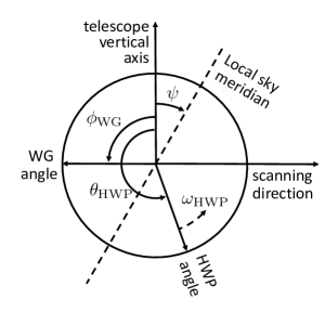
Figure 15: LSPE-SWIPE Stokes polarimeter angles as seen from the boresight. The dashed line is the instantaneous local sky meridian; the telescope vertical axis is tilted by an angle $\psi$ with respect to the sky meridian, and is orthogonal to the scanning direction. The wire grid inside the cryostat is oriented at an angle $\phi_{\text{WG}}$ orthogonal to the vertical axis; the HWP is spinning with angular velocity $\omega_{\text{HWP}}$, and forms an angle $\theta_{\text{HWP}}=\omega_{\text{HWP}}t$ with the telescope vertical axis.

In an ideal Stokes polarimeter, the power hitting the detector can be computed as the first element of the Stokes vector obtained from the combination of Mueller matrices, taking into account both the rotating HWP and the WG polarizer:

$$S_{\text{out}}=M_{\text{rot}}^{-1}(\phi_{\text{WG}})M_{\text{WG}}M_{\text{rot}}(\phi_{\text{WG}})M_{\text{rot}}^{-1}(\theta_{\text{HWP}})M_{\text{HWP}}M_{\text{rot}}(\theta_{\text{HWP}})M_{\text{rot}}(\psi)S_{\text{sky}}$$

where $S_{\text{sky}}$ is the Stokes vector $(I,Q,U,V)$ of the observed direction in the sky; $M_{\text{rot}}$ is the rotation Mueller matrix; $M_{\text{HWP}}$ is the HWP Mueller matrix; $M_{\text{WG}}$ is the wire grid Mueller matrix; $\psi$ is the angle between the local meridian and the telescope vertical axis; $\theta_{\text{HWP}}=\omega_{\text{HWP}}t$ is the rotation angle, with respect to telescope vertical axis, of the HWP which rotates with $\omega_{\text{HWP}}$ angular velocity; $\phi_{\text{WG}}$ is the wire grid rotation angle with respect to telescope vertical axis ($0\mathrm{°}$ or $90\mathrm{°}$ in the case of SWIPE, for reflected and transmitted radiation); and $S_{\text{out}}$ is the resulting Stokes vector, of which the $I_{\text{out}}$ term is the power hitting the detector. Figure 15 illustrates the angles definition. Expanding the equation, we have

$$I_{\text{out}}=\frac{1}{2}\left(AI_{\text{sky}}(\hat{n}(t))+BQ_{\text{sky}}(\hat{n}(t))+CU_{\text{sky}}(\hat{n}(t))\right)$$ (2.1)

with

$$A = 1$$

$$B = \cos(4\omega_{\text{HWP}}t+2(\psi(t)-\phi_{\text{WG}}))$$

$$C = \sin(4\omega_{\text{HWP}}t+2(\psi(t)-\phi_{\text{WG}}))$$

where $\hat{n}(t)$ is the observed direction, and we have made explicit the time dependence.

The HWP angular velocity is constrained by the detectors’ time constant, while the payload scanning speed is constrained by the telescope angular response. The derivation of baseline parameter for LSPE-SWIPE is described in Appendix A, and the results are reported in table 13. Notably, the scanning speed is $\omega_{\text{payload}}\simeq$0.7\text{\thinspace}\mathrm{\SIUnitSymbolDegree}\thinspace\mathrm{s}^{-1}$$ and the HWP angular velocity is $\omega_{\text{HWP}}=$3.14\text{\thinspace}\mathrm{r}\mathrm{a}\mathrm{d}\thinspace\mathrm{s}^{-1}$$.

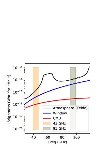
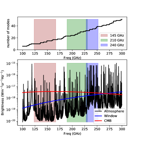
Figure 16: Left: LSPE-Strip bands and expected brightness from atmosphere, cryostat window and CMB. Top-right: LSPE-SWIPE number of modes coupled to the multi-moded optical assembly, as function of frequency. The three bands centered at 145, 210, $240\text{\thinspace}\mathrm{G}\mathrm{H}\mathrm{z}$ are also shown. Bottom-right: LSPE-SWIPE bands and expected brightness from atmosphere at balloon altitude, cryostat window and CMB. For both Strip and SWIPE the brightness values don’t include telescope and coupling efficiency.

2.3.7 Detectors

LSPE-SWIPE adopts TES detectors. In order to take advantage of the multi-moded coupling, radiative power propagated from the feedhorns into the mode-filtering waveguides must be absorbed by the detector with as low an impedance mismatch as possible for all the propagated modes. One way to fulfill this requirement is to compress the effective wavelengths of the coupled modes into a narrower bandwidth by progressively re-enlarging the waveguide cross-section into a larger terminated cavity (flared waveguide), where a 15 mm large spider-web absorber collects the power for detection by the TES. This solution has been validated through HFSS, providing a mode-dependent, frequency-dependent $S_{11}$ scattering parameter evaluation of the pixel assembly along the path from the waveguide to the absorber. The relative $S_{11}$-parameter dispersion for the $150\text{\thinspace}\mathrm{G}\mathrm{H}\mathrm{z}$ band is about 2% over the coupled modes and frequencies, with an average return loss of $-$22.6\text{\thinspace}\mathrm{d}\mathrm{B}$$ when the cavity termination is set to a quarter of the average free-space wavelength of the band collected by the detector, and the absorber impedance is $\sim$300\text{\thinspace}\mathrm{\SIUnitSymbolOhm}$$. This result, to be validated also through experimental verification of the pixel performance, is used here to support the hypothesis that the main impact of the broadband performance evaluation for SWIPE is the variable number of modes $N_{\text{modes}}(r_{\text{wg}},\nu)$ coupled by the waveguide when fed with broadband radiation. Figure 16 illustrates the coupled modes as a function of frequency, and the selected bands; in the bottom-right panel, it shows the power entering the system, with contribution from the CMB, the atmosphere and the cryostat window (for Strip in the bottom-left panel). These are the input to the noise calculation analysis reported in section 3.2 and in table 4.

The TES bolometer is a single Si chip $15\times$15\text{\thinspace}\mathrm{m}\mathrm{m}^{2}$$ with Au absorber deposited on a central free-standing Si₃N₄ membrane, $1\text{\thinspace}\mathrm{\SIUnitSymbolMicro}\mathrm{m}$ thick and $10\text{\thinspace}\mathrm{m}\mathrm{m}$ diameter. After the TES and Au absorber film have been grown, the membrane is first etched in the shape of a 8 mm diameter circular spider-web supported by 32 narrow legs and then suspended by means of Deep Reactive Ion Etching of the silicon beneath. The TES is located aside the circular spider-web and is in strong electronic contact with the external perimeter of the gold absorber. The TES consists of 120 nm of a Au-Ti bilayer, which is manufactured taking care to maintain a process temperature profile below $100\text{\thinspace}\mathrm{\SIUnitSymbolCelsius}$, to ensure a superconducting to normal transition at $T_{c}=500-$550\text{\thinspace}\mathrm{m}\mathrm{K}$$. In fact, it has been observed that high process temperatures reduce $T_{c}$ towards its bulk value of $350-$400\text{\thinspace}\mathrm{m}\mathrm{K}$$, as demonstrated in [87]. These operating temperatures represent an optimal compromise between the SWIPE’s bath temperature of $300\text{\thinspace}\mathrm{m}\mathrm{K}$ and the detector saturation limits due to the high optical power (order of $10\text{\thinspace}\mathrm{p}\mathrm{W}$) of the multi-mode configuration. The thermal conductance $G$, in the range of $65-$100\text{\thinspace}\mathrm{p}\mathrm{W}\thinspace\mathrm{K}^{-1}$$, was measured in the first prototypes that have been operated at a base temperatures of about $350\text{\thinspace}\mathrm{m}\mathrm{K}$. The effective time constants in the Electro-Thermal Feedback (ETF) regime were evaluated from the frequency response to a sinusoidal sweep excitation to be $20-$33\text{\thinspace}\mathrm{m}\mathrm{s}$$, about a factor $2-3$ larger than the ones expected by the model. In these working points the thermal fluctuation noise equivalent power, NEP, is about $3\text{\times}{10}^{-17}\text{\thinspace}\mathrm{W}\thinspace\mathrm{H}\mathrm{z}^{-1/2}$ (see section 3.2 for details).

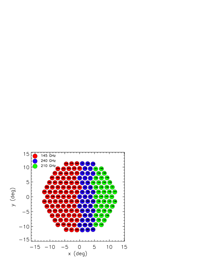
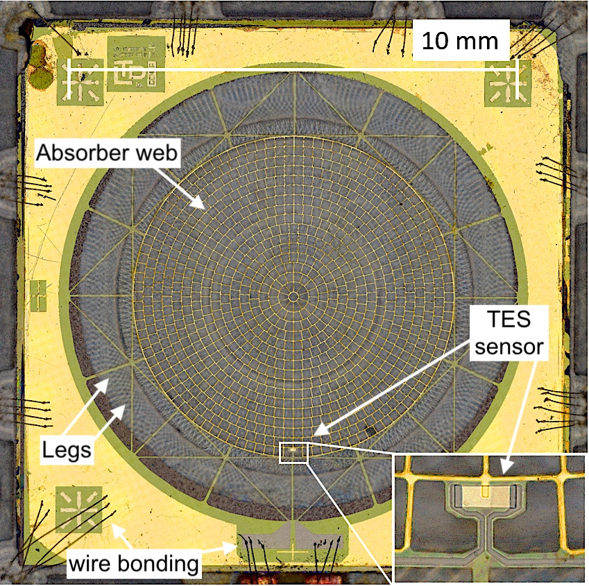
Figure 17: Left: distribution of detectors in one of the two equivalent focal planes. The payload rotates so that the scanning direction is along the x-axis. Right: a LSPE-SWIPE large spider-web TES bolometer integrated in the backshort of the microwave cavity.

The left panel of figure 17 shows the distribution of detectors in one of the two equivalent focal planes. The payload rotates so that the scanning direction is along the $x$ axis in the figure. The right panel of figure 17 shows the LSPE-SWIPE large spider-web TES bolometer integrated in the backshort of the microwave cavity.

2.3.8 Readout

The 326 TES bolometers are read-out by Superconducting Quantum Interference Devices (SQUIDs) using a Frequency-Domain Multiplexing scheme (FDM), with each DC-SQUID sensing 16 TES [88]. In the FDM scheme a group of detectors is readout with a single SQUID by connecting in parallel several RLC chains in which R is given by the TES variable resistance, and the LC filters define different frequencies. A single signal containing all the different frequencies is therefore needed to bias all TESs simultaneously. The detectors modulate the signal which is in turn sent to the SQUID input, amplified and demodulated by digital electronics. The multiplexing tones are in the range from 100 kHz to 2 MHz, to be faster than the bolometers’ response but below the cut-off frequency of the readout, the latter determined mainly by the length of the cables inside the cryostat. In this range we can safely accommodate 16 tones that readout TESs coupled to detectors at all the three bands. Some channels are coupled to blind detectors and/or calibration resistor to monitor gain fluctuations of the readout chain.

The readout electronic chain is composed of a cold section inside the cryostat, at the same temperature of the detectors, and a warm section, outside the cryostat. The entire chain is composed, going from the lowest to the highest temperature, of the LC filters and the bias resistors board, the SQUIDs boxes, the SQUID control unit and the warm electronics (see figure 18).

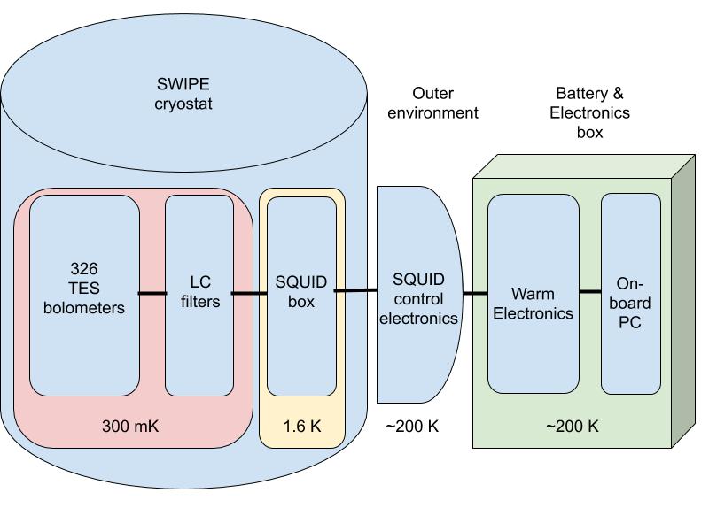
Figure 18: Schematic of the LSPE-SWIPE readout with the indication of the temperatures of the different stages.

LC filters. The LC filters necessary to the frequency domain multiplexing are assembled on dedicated boards placed at $300\text{\thinspace}\mathrm{m}\mathrm{K}$ in close proximity to the TESs. The filters are composed of a niobium inductor fabricated by optical lithography coupled to a commercial Surface Mount Device (SMD) capacitor [89]. Given the inductance $L\approx$15\text{\thinspace}\mathrm{\SIUnitSymbolMicro}\mathrm{H}$$, the capacitors are chosen in order to give resonance frequencies in the $200\text{\thinspace}\mathrm{k}\mathrm{H}\mathrm{z}$ to $2\text{\thinspace}\mathrm{M}\mathrm{H}\mathrm{z}$ range. Bolometers are connected to the LC board with shielded twisted pair wires. Furthermore the TES bias resistor is also placed on the board to minimize Johnson noise. Each board hosts three LC chains to read a quarter of focal plane. Four such boards are used for each focal plane for a total of eight boards.

SQUID boxes. Each LC board is connected with a custom low-inductance flat cable to a SQUID box placed at $1.6\text{\thinspace}\mathrm{K}$. Each box is used to thermalize and shield three SQUIDs, for a total of 24 SQUIDs for the two focal planes. SQUIDs convert the modulated current signal into a modulated and amplified voltage signal which in turn is sent to a further amplification stage outside the cryostat. The SQUIDs that are baselined for LSPE/SWIPE are 6-stage SQUID arrays from VTT (model K3B) with critical current $I_{c}\approx$65\text{\thinspace}\mathrm{\SIUnitSymbolMicro}\mathrm{A}$$, input inductance $2$ nH and a transimpedance of $30$ to $50\text{\thinspace}\mathrm{V}\thinspace\mathrm{A}^{-1}$ typically. The flux coupling and noise are $36\text{\thinspace}\mathrm{\SIUnitSymbolMicro}\mathrm{A}\thinspace\Phi_{\mathrm{0}}^{-1}$ and $\lesssim$0.1\text{\thinspace}\mathrm{\SIUnitSymbolMicro}\Phi_{\mathrm{0}}\thinspace\mathrm{H}\mathrm{z}^{-1/2}$$ respectively ($\Phi_{0}$ being the magnetic flux quantum). Two different coupling strengths can be selected for the feedback coil: $M_{f}^{-1}\simeq$40\text{\thinspace}\mathrm{\SIUnitSymbolMicro}\mathrm{A}\thinspace\Phi_{\mathrm{0}}^{-1}$$ and $M_{f}^{-1}\simeq$90\text{\thinspace}\mathrm{\SIUnitSymbolMicro}\mathrm{A}\thinspace\Phi_{\mathrm{0}}^{-1}$$.

SQUID Control Units. The SQUID control units (SCUs) are placed outside the cryostat and perform the main following tasks: (i) they provide the SQUID bias signal (which will be set at the SQUID operating temperature and will be tuned in flight); (ii) they linearize SQUID response by means of a flux-locked loop (FLL hereafter); and (iii) they host the amplification stage needed to amplify the SQUID output voltage before the digitizing stage. The desired amplification is achieved in two stages, in order to obtain the desired bandwidth and to minimize the noise referred to the amplifier’s input. The SQUID output is first amplified by a very low noise preamplifier based on a discrete JFET (IF3602) input differential cascode architecture, followed by a low noise CMOS operational amplifier (OPA301). The equivalent input noise density is $0.6\text{\thinspace}\mathrm{n}\mathrm{V}\thinspace\mathrm{H}\mathrm{z}^{-1/2}$ and the bandwidth extends up to at least 2 MHz [90].

Warm readout. The warm readout boards contain the ADCs (LTM9001IV) and the DACs (LTC1668IG) that are used to generate the sum of sinusoids to bias the TES detectors and to digitize the modulated output. They in turn perform the digital demodulation and the data compression. They perform these operations by means of a system-on-module board hosting a FPGA and an ARM microprocessor (MitySOM 5CSX System-On-Module). Each board, with a single SOC, runs two readout chains, therefore the complete readout system is composed of a total of 12 boards in a 6U standard, placed in a custom aluminum crate that provides the mechanical support and dissipates the generated heat. Each warm readout board builds the packets that are sent to the on-board computer to be assembled in one single event.

3 Sensitivity of instruments

Realistic simulations of the observations are obtained for LSPE by means of noise estimation for Strip and SWIPE, and propagated from time-ordered data to maps using the instrument simulators described in detail in Appendix B.

3.1 LSPE-Strip noise estimation

We model the noise of the Strip polarimeters as the sum of a white noise plus a $1/f^{\alpha}$ component, so that the post-detection power spectrum can be written as:

$$P(f)=\sigma^{2}\left[1+\left(\frac{f_{\mathrm{knee}}}{f}\right)^{\alpha}\right],$$ (3.1)

where the knee frequency, $f_{\mathrm{knee}}$, is the frequency where the white noise and the $1/f^{\alpha}$ components contribute equally ($P(f_{\mathrm{knee}})=2\sigma^{2}$). Previous experience (QUIET, WMAP, Planck-LFI) shows that this simple model provides a very good first-order description of the noise properties of HEMT-based coherent devices. The standard deviation of the white noise component of the $Q$ and $U$ Stokes parameters measured by each Strip polarimeter in antenna temperature is given by:

$$\Delta T_{\mathrm{r.m.s.}}=\frac{1}{\sqrt{2}}\frac{T_{\mathrm{sys}}}{\sqrt{\Delta\nu\thinspace\tau}},$$ (3.2)

where $T_{\mathrm{sys}}$ is the total intensity detected by the polarimeters (sky signals, emissions from the optical components and receiver noise temperature), $\Delta\nu$ is the receiver bandwidth and $\tau$ is the integration time. The factor $1/\sqrt{2}$ in equation 3.2 results from the polarimeter correlation architecture and it is explained in [91] and section 4 of [92]. In table 2 we detail the budget leading to the current estimate of the average receiver white noise performance.

	$43\text{\thinspace}\mathrm{G}\mathrm{H}\mathrm{z}$	$95\text{\thinspace}\mathrm{G}\mathrm{H}\mathrm{z}$
Sky signals in antenna temperature
Atmospheric emission at Zenith $\left($\text{\thinspace}\mathrm{K}_{RJ}$\right)^{1}$	$16.3$	$19.0$
CMB $\left($\text{\thinspace}\mathrm{K}_{RJ}$\right)$	$1.8$	$1.1$
Noise contributions
Mirror emission $\left($\text{\thinspace}\mathrm{K}_{RJ}$\right)^{2}$	$3.0$	$3.0$
Window $\left($\text{\thinspace}\mathrm{K}_{RJ}$\right)^{3}$	$3.0$	$8.0$
Filters $\left($\text{\thinspace}\mathrm{K}_{RJ}$\right)^{3}$	$2.0$	$3.0$
Feed system $\left($\text{\thinspace}\mathrm{K}_{RJ}$\right)^{4}$	$0.5$	$0.5$
Polarimeter noise $\left($\text{\thinspace}\mathrm{K}_{RJ}$\right)^{5}$	$34.0$	$104.2$
System temperature6, $T_{\mathrm{sys}}$ $\left($\text{\thinspace}\mathrm{K}_{RJ}$\right)$	$61.7$	$140.0$
1-second sensitivity per polarimeter7
Antenna temperature $\left($\text{\thinspace}\mathrm{\SIUnitSymbolMicro}\mathrm{K}_{RJ}\thinspace\mathrm{s}^{1/2}$\right)$	$514.6$	$1139.5$
Thermod. temperature $\left($\text{\thinspace}\mathrm{\SIUnitSymbolMicro}\mathrm{K}_{CMB}\thinspace\mathrm{s}^{1/2}$\right)$	$539.7$	$1431.4$

¹Simulated with am Atmospheric Model code, based on partial water vapor measurements
²Assumes $300\text{\thinspace}\mathrm{K}$ physical temperature and 1% mirror emissivity
³Estimated using electromagnetic simulations ($60\text{\thinspace}\mathrm{m}\mathrm{m}$ window thickness)
⁴Assumes $20\text{\thinspace}\mathrm{K}$ physical temperature and $\sim$0.1\text{\thinspace}\mathrm{d}\mathrm{B}$$ insertion loss
⁵Measured during unit-level tests
⁶Calculated assuming a constant zenith angle of $20\text{\thinspace}\mathrm{\SIUnitSymbolDegree}$ during the whole survey.
⁷Calculated assuming the receiver bandwidth reported in table 1 and a constant zenith angle of $20\text{\thinspace}\mathrm{\SIUnitSymbolDegree}$ during the whole survey.

Table 2: White noise sensitivity budget of Strip polarimeters

We now discuss briefly the low-frequency properties of the noise spectrum and show how the expected impact from $1/f^{\alpha}$ noise components is small. In our measurements we expect two main sources of noise fluctuations on long time scales: (i) fluctuations in the receiver gain and (ii) variations in the atmospheric load. Both contribute to the $1/f^{\alpha}$ shape of the noise spectrum at low frequencies. Strip polarimeters have a very low susceptibility to gain fluctuations and $1/f^{\alpha}$ noise contributes in polarization only at frequencies less than few tens of mHz.

This stability is the result of the differential nature of the receiver that allows one to recover the $Q$ and $U$ Stokes parameters by differentiating signals having essentially the same intensity, thus effectively canceling out common modes. The penalty is that these detectors are practically blind to the CMB total intensity, as these measurements retain all the common-mode fluctuations and are characterized by knee frequencies of the order of several Hz.

If we assume zero or negligible polarization in the atmospheric signal, then we can neglect, to first order, also the effect of $1/f^{\alpha}$ fluctuations in the atmospheric load. These will contaminate polarization measurements only through any leakage from total intensity to polarization that could be present in our receivers and that will be caused mainly by asymmetries in the polarizer-OMT system. Considering that our current estimates from OMT laboratory measurements [46] indicate a leakage of the order of $\sim 0.01\%$ this effect is likely to be negligible. We are currently working on a simulation framework that will model the expected fluctuations in the atmosphere brightness temperature and their effect of the sky polarization measurement and will allow us to quantify the impact of this systematic effect.

3.2 LSPE-SWIPE noise estimation

The LSPE-SWIPE detector’s noise is given by the combination of photon noise, detector thermal noise, readout electronics noise, and the effect of cosmic rays.

The photon noise is computed assuming that the incoming radiation is the composition of: (i) the CMB, a $2.725\text{\thinspace}\mathrm{K}$ black-body; (ii) the residual atmosphere, as computed from the am Atmospheric Model [93] assuming a pessimistic residual ambient pressure of $10\text{\thinspace}\mathrm{mbar}$ and a zenith angle of $45\text{\thinspace}\mathrm{\SIUnitSymbolDegree}$; (iii) the cryostat window, as a $240\text{\thinspace}\mathrm{K}$ grey-body with emissivity computed assuming a layer of Mylar [94], thickness $t=$1\text{\thinspace}\mathrm{m}\mathrm{i}\mathrm{l}$$ ($\sim$25.4\text{\thinspace}\mathrm{\SIUnitSymbolMicro m}$$) with $n_{r}=1.57$ and loss tangent $\tan\delta=2.25\times 10^{-3}$. The window emissivity is computed as $\varepsilon_{\text{window},\nu}=1-\exp(-2\pi n_{r}(t/\lambda)\tan\delta)$, where $\lambda$ is the wavelength [95]. The loading from the IR filters, lens, HWP and other cryogenic elements is computed to be negligible with respect to CMB, window and atmosphere. Following [96], for each component, the power on the detector is computed as

$$P=\int f_{\nu}\eta A\Omega I_{\nu}d\nu$$ (3.3)

where $f_{\nu}$ defines the filter pass-band; $\eta$ is the instrument efficiency, which includes a factor 0.5 to take into account the selection of one polarization by means of the wire grid; $I_{\nu}$ is the spectral brightness ($\text{\thinspace}\mathrm{W}\thinspace\mathrm{m}^{-2}\thinspace\mathrm{s}\mathrm{r}^{-1}\thinspace\mathrm{H}\mathrm{z}^{-1}$) of the component; $A\Omega$ is the throughput, estimated as $N_{\text{modes}}\lambda^{2}$, with $N_{\text{modes}}$ the number of electromagnetic modes coupled to each detector. The photon noise equivalent power in $\text{\thinspace}\mathrm{W}\thinspace\mathrm{H}\mathrm{z}^{-1/2}$ of a beam filling source is computed as:

$$\text{NEP}^{2}_{\text{ph}}=2\int f_{\nu}\eta A\Omega I_{\nu}h\nu\left(1+\frac{f_{\nu}\eta c^{2}I_{\nu}}{h\nu^{3}}\right)d\nu.$$ (3.4)

The total photon noise $\text{NEP}_{\text{ph-total}}$ is the quadrature sum of the photon noise from the CMB, $\text{NEP}_{\text{ph-CMB}}$, the atmosphere, $\text{NEP}_{\text{ph-atm}}$, and the window $\text{NEP}_{\text{ph-window}}$.

The detector’s thermal noise also depends on the power load. The higher the load, the higher must be the thermal conductivity $G$ which links the detector to the thermal bath, in order to avoid the transitioning of the TES to normal state. Following [97], the detector’s thermal noise is computed as

$$\text{NEP}_{\text{detector}}=\sqrt{4k_{B}T_{c}^{2}GF}$$ (3.5)

where $k_{B}$ is the Boltzmann constant, $T_{c}=$550\text{\thinspace}\mathrm{m}\mathrm{K}$$ is the critical temperature, and $F=\left[0.5;1\right]$ takes into account non-equilibrium effects in TES (we assume a pessimistic $F=1$). The optimal thermal conductivity is

$$G=\frac{nP_{\text{sat}}T_{c}^{n-1}}{T_{c}^{n}-T_{\text{bath}}^{n}}$$ (3.6)

where $n=3.2$ takes into account the thermal dependence of the conductivity, $T_{\text{bath}}=$300\text{\thinspace}\mathrm{m}\mathrm{K}$$ is the temperature of the thermal bath, and $P_{\text{sat}}=2.5\thinspace P_{\text{total}}$ is the saturation power, with a 2.5 safety factor ($P_{\text{total}}$ being the total optical power on the detector). Given that the detectors are all built with the same characteristics, we set the detector noise (equation 3.5) using the highest value among the thermal conductivity of the 3 bands, $G_{\text{max}}$. With this highest value, we compute the typical detector noise, NET${}_{\text{detector,max}}$. Combining equation 3.5 with 3.6 and 3.3, it can be noted that $\text{NEP}_{\text{detector}}$ is proportional to $(A\Omega)^{1/2}$.

Source	Value	Value at SQUID	Factor to	Note	Noise on detector
	at source	input $\left($\text{\thinspace}\mathrm{p}\mathrm{A}\thinspace\mathrm{H}\mathrm{z}^{-1/2}$\right)$	SQUID input		$\left($\text{\thinspace}\mathrm{a}\mathrm{W}\thinspace\mathrm{H}\mathrm{z}^{-1/2}$\right)$
SQUID noise	$10\text{\thinspace}\mathrm{p}\mathrm{A}\thinspace\mathrm{H}\mathrm{z}^{-1/2}$	$10$	1	(a)	10
DAC LTC1668	$50\text{\thinspace}\mathrm{p}\mathrm{A}\thinspace\mathrm{H}\mathrm{z}^{-1/2}$	$<5$	$1/10$	(b)	$<5$
Preamplifier	$0.6\text{\thinspace}\mathrm{n}\mathrm{V}\thinspace\mathrm{H}\mathrm{z}^{-1/2}$	$6$	$\sim 100$ V/A	(c)	6
Cabling	$0.3\text{\thinspace}\mathrm{n}\mathrm{V}\thinspace\mathrm{H}\mathrm{z}^{-1/2}$	$3$	$\sim 100$ V/A	(c)	3
Bias resistor	$2.6\text{\thinspace}\mathrm{p}\mathrm{A}\thinspace\mathrm{H}\mathrm{z}^{-1/2}$	2.6	1	(d)	$\sim 2.5-4.0$
Total				(e)	$15-20$

Table 3: Contribution of selected readout electronics noise source s to the NEP budget. (a) Typical noise of SQUID arrays currently being considered for the LSPE readout, given by the flux noise multiplied by the SQUID input coil coupling; (b) the DAC noise is reduced at the SQUID input by a suitable resistive divider; (c) the noise of the warm preamplifier is referenced to the SQUID input by using the SQUID transimpedence; the number reported here is the typical for the 6-series array SQUID being considered for the readout; (d) current noise of the bias resistor at $300\text{\thinspace}\mathrm{m}\mathrm{K}$, with $R_{b}=$0.1\text{\thinspace}\mathrm{\SIUnitSymbolOhm}$$, and assuming the normal state resistance $R_{N}=$1.0\text{\thinspace}\mathrm{\SIUnitSymbolOhm}$$, and a TES resistance around $R_{N}/2$ in ETF; (e) assumes a TES responsivity of $-\sqrt{2}/V_{\rm bias}$ with $V_{\rm bias}\approx 1-2$ $\text{\thinspace}\mathrm{\SIUnitSymbolMicro}\mathrm{V}$: the noise at squid input has to be divided by the responsivity to get the NEP at detector.

Band (GHz)	145	210	240
bandwidth	30%	20%	10%
$N_{\text{modes}}$1	[10;13.1;17]	[23;27.0;32]	[32;34.5;39]
$A\Omega$ $\left($\text{\thinspace}\mathrm{m}^{2}\thinspace\mathrm{s}\mathrm{r}$\right)$	$N_{\text{modes}}\lambda^{2}$
efficiency $\eta$	0.3	0.25	0.25
Power on cryostat entrance
$P_{\text{CMB}}$ $\left($\text{\thinspace}\mathrm{p}\mathrm{W}$\right)$	9.1	7.7	3.9
$P_{\text{atm}}$ $\left($\text{\thinspace}\mathrm{p}\mathrm{W}$\right)$	0.9	1.9	9.8
$P_{\text{window}}$ $\left($\text{\thinspace}\mathrm{p}\mathrm{W}$\right)$	1.0	2.8	2.4
$P_{\text{total}}$ $\left($\text{\thinspace}\mathrm{p}\mathrm{W}$\right)$	11.0	12.4	16.1
Power on detector
$P_{\text{total-detector}}$ $\left($\text{\thinspace}\mathrm{p}\mathrm{W}$\right)$	3.3	3.1	4.0
Noise on detector
NEP${}_{\text{ph-CMB}}$ $\left($\text{\thinspace}\mathrm{a}\mathrm{W}\thinspace\mathrm{H}\mathrm{z}^{-1/2}$\right)$	23.5	23.3	17.6
NEP${}_{\text{ph-atm}}$ $\left($\text{\thinspace}\mathrm{a}\mathrm{W}\thinspace\mathrm{H}\mathrm{z}^{-1/2}$\right)$	8.4	12.3	34.1
NEP${}_{\text{ph-window}}$ $\left($\text{\thinspace}\mathrm{a}\mathrm{W}\thinspace\mathrm{H}\mathrm{z}^{-1/2}$\right)$	7.8	14.2	13.9
NEP${}_{\text{ph-total}}$ $\left($\text{\thinspace}\mathrm{a}\mathrm{W}\thinspace\mathrm{H}\mathrm{z}^{-1/2}$\right)$	26.1	29.9	40.8
$G$ $\left($\text{\thinspace}\mathrm{p}\mathrm{W}\thinspace\mathrm{K}^{-1}$\right)$	56.1	52.7	68.4
$G_{\text{max}}$ $\left($\text{\thinspace}\mathrm{p}\mathrm{W}\thinspace\mathrm{K}^{-1}$\right)$	68.4
NEP${}_{\text{detector}}$ $\left($\text{\thinspace}\mathrm{a}\mathrm{W}\thinspace\mathrm{H}\mathrm{z}^{-1/2}$\right)$	30.6	29.7	33.8
NEP${}_{\text{detector,max}}$ $\left($\text{\thinspace}\mathrm{a}\mathrm{W}\thinspace\mathrm{H}\mathrm{z}^{-1/2}$\right)$	33.8
NEP${}_{\text{readout}}$ $\left($\text{\thinspace}\mathrm{a}\mathrm{W}\thinspace\mathrm{H}\mathrm{z}^{-1/2}$\right)$	20
NEP${}_{\text{total}}$ $\left($\text{\thinspace}\mathrm{a}\mathrm{W}\thinspace\mathrm{H}\mathrm{z}^{-1/2}$\right)$	47.2	49.4	56.6
Optical noise
NEP${}_{\text{optical-total}}$ $\left($\text{\thinspace}\mathrm{a}\mathrm{W}\thinspace\mathrm{H}\mathrm{z}^{-1/2}$\right)$	157	197	226
NET $\left($\text{\thinspace}\mathrm{\SIUnitSymbolMicro}\mathrm{K}_{CMB}\thinspace\mathrm{s}^{1/2}$\right)$	11.4	12.3	26.2
margin $m$ $\left(\%\right)$	5	20	20
NET${}_{\text{eff}}$ $\left($\text{\thinspace}\mathrm{\SIUnitSymbolMicro}\mathrm{K}_{CMB}\thinspace\mathrm{s}^{1/2}$\right)$	12.6	15.6	31.4
1The number of modes varies across the band (see figure 16), with less modes in the lower side of the band, and more modes in the higher side. The three values in the square brackets indicate the number of modes at the minimum frequency of each band, the average across the band, and number at the maximum frequency of each band.

Table 4: LSPE-SWIPE detectors radiative power and noise estimation. See text for details.

The readout electronics chain is designed to keep its noise NEP${}_{\rm readout}\lesssim$20\text{\thinspace}\mathrm{a}\mathrm{W}\thinspace\mathrm{H}\mathrm{z}^{-1/2}$$, sub-dominant with respect to photon noise $\text{NEP}_{\text{ph-total}}$ and detector thermal noise $\text{NEP}_{\text{detector}}$. The known noise sources are first evaluated at their origin, then converted to values at the SQUID input by applying the appropriate conversion factors, and finally converted to equivalent noise on the detector by means of the TES current responsivity $R_{I}$. To do so, we take into account the low frequency limit of $R_{I}$ in the case of strong electro-thermal feedback, i.e. $R_{I}\simeq-\sqrt{2}/V_{\rm bias}$, where $V_{\rm bias}$ is the TES bias voltage, and the $\sqrt{2}$ factor originates from the AC bias in the multiplexing scheme (see the discussion in the appendix of [98] for further details). The numbers quoted in table 3 are obtained assuming the expected voltage bias of $V_{\rm bias}\approx 1-$2\text{\thinspace}\mathrm{\SIUnitSymbolMicro}\mathrm{V}$$. We take into consideration the following noise sources: the SQUID current noise, the DAC current noise, the SQUID preamplifier noise and the Johnson noise of bias resistor and cabling between the cold (inside the cryostat) and the warm (outside) section of the electronics. In table 3 we quote their typical values together with the factor needed for comparison at the SQUID input. See [99] for further details on the assumed noise model. The total readout current noise NEP_readout is computed as the quadrature sum of these contributions.

The total noise equivalent power, NEP${}_{\text{total}}$, is computed by quadrature sum of the photon noise from different sources, the detector thermal noise and the readout noise. The optical noise, which converts the noise on the detector to noise at the instrument aperture, taking efficiency into account, is computed as

$$\text{NEP}_{\text{optical-total}}=\text{NEP}_{\text{total}}/\eta$$

Results of this calculation are converted to $\text{\thinspace}\mathrm{\SIUnitSymbolMicro}\mathrm{K}_{CMB}\thinspace\mathrm{s}^{1/2}$ as:

$$\text{NET}=\frac{T_{\text{CMB}}}{\int f_{\nu}A\Omega B(T_{\text{CMB}})\frac{xe^{x}}{e^{x}-1}dx}\frac{\text{NEP}_{\text{optical-total}}}{\sqrt{2}}$$ (3.7)

where $B(T_{\text{CMB}})$ is the CMB black-body brightness, $x=h\nu/(k_{B}T_{\text{CMB}})$ is the reduced frequency, and the factor $1/\sqrt{2}$ takes into account the conversion from $\text{\thinspace}\mathrm{\SIUnitSymbolMicro}\mathrm{K}_{CMB}\thinspace\mathrm{H}\mathrm{z}^{-1/2}$ to $\text{\thinspace}\mathrm{\SIUnitSymbolMicro}\mathrm{K}_{CMB}\thinspace\mathrm{s}^{1/2}$. Notably, the photon noise NEP (as the thermal noise) is proportional to $(A\Omega)^{1/2}$, while the NET is inverse proportional to $(A\Omega)^{1/2}$ and thus to $N_{\text{modes}}^{1/2}$. This is the advantage of multi-moded detectors: higher photon noise, which relaxes the detector noise requirement, and lower NET. Background and noise calculation results are reported in table 4. In order to take into account possible effects such as contamination by cosmic rays (see next section), atmospheric background variation, detectors yield, detector excess noise, and other unexpected effects, we also report the margin $m$ value and the effective noise,

$$\text{NET}_{\text{eff}}=\text{NET}(1+m),$$

which we use as input in the instrument simulator, for the results reported in section 5. The margin $m$ is not the same for all channels, due to the largest uncertainty in the atmospheric modeling in the highest frequencies. In SWIPE, the $1/f$ noise term has negligible impact, due to the polarization modulation by means of the HWP. Measurements of the detector noise power spectra show the typical behaviour of $1/f$ evident at low frequency, on top of a flat spectrum, with an high frequency roll-off due to the detectors’ time constants cut-off.

3.2.1 Cosmic rays rate

TES detectors are sensitive to any form of energy deposited on the absorber, including the effect of cosmic rays. The flux of primary cosmic rays in the upper atmosphere is fairly well known, as well as its dependence on the latitude and on the solar cycles. We evaluated the expected rate of interactions by cosmic rays in the upper atmosphere (altitude $40\text{\thinspace}\mathrm{k}\mathrm{m}$) along the orbit of SWIPE by using the measured fluxes and simulating the interactions of primary protons and alphas on the SWIPE cryostat, instrument and focal plane. An energy-integrated flux of $1.5\text{\thinspace}\mathrm{p}\mathrm{a}\mathrm{r}\mathrm{t}\mathrm{i}\mathrm{c}\mathrm{l}\mathrm{e}\mathrm{s}\thinspace\mathrm{c}\mathrm{m}^{-2}\thinspace\mathrm{s}^{-1}$ is obtained at the minimum of the solar activity cycle, decreasing by a factor $\approx 2.5$ at the solar activity maximum.

We assume that cosmic rays release a signal in the bolometers whenever they interact with the gold-plated spider-web structure. By using the geometrical characteristics of our spider-web bolometers (diameter $8\text{\thinspace}\mathrm{m}\mathrm{m}$, fill factor $8\%$) we estimate an interaction rate of $60\text{\thinspace}\mathrm{m}\mathrm{H}\mathrm{z}$ per bolometer, giving roughly a $1\text{\thinspace}\mathrm{H}\mathrm{z}$ rate of interaction per readout chain, given that the bolometers are multiplexed in groups of 16. The $60\text{\thinspace}\mathrm{m}\mathrm{H}\mathrm{z}$ rate is reasonable once compared with the (inverse of the) bolometer time constant, nevertheless suitable algorithms for cosmic ray hit identification and removal must be implemented. These algorithms also subtract the long tail after the glitch in the data. In a typical case, after a glitch, it is impossible to recover the first part of the tail, equal to $[5;10]\thinspace\tau_{\text{LP}}$. With a rate of one event every $16.7\text{\thinspace}\mathrm{s}$ and a time constant $\tau_{\text{LP}}=$30\text{\thinspace}\mathrm{m}\mathrm{s}$$, this correspond to removing between 1 and 2% of the data, well within our margins.

4 Systematic effects and calibration

In this section we present the most relevant systematic effects for the two instruments, with particular focus on the systematic effects critical for the measurement of the CMB polarization. We also set requirements on the knowledge of the most important instrumental parameters, and discuss the calibration plans.

4.1 LSPE-Strip systematic effects

Here we provide a brief summary of the Strip susceptibility to systematic effects, deferring to forthcoming papers a more detailed treatment.

Systematic effects budget.

We start by setting a top-level requirement on the maximum uncertainty from systematic effects on a single sky pixel having the size of the Q-band optical angular resolution. In general we want this uncertainty to be much less than that imposed by the white noise. Following the approach already adopted for Planck-LFI [100, 101] we set this limit to 5% of the white noise level as a goal and 10% of the white noise level as a requirement. In table 5 we provide a list of systematic effects that could affect Strip polarimetric measurements and goal/requirement values for the upper limit in the systematic uncertainty. The detailed breakdown has been defined according to our best current knowledge of the instrumental properties.

Strip systematic effect	Goal	Requirement
	($\text{\thinspace}\mathrm{\SIUnitSymbolMicro}\mathrm{K}$)	($\text{\thinspace}\mathrm{\SIUnitSymbolMicro}\mathrm{K}$)
$I\rightarrow Q/U$ leakage	0.030	0.050
$Q\rightarrow U$ and $U\rightarrow Q$ leakage	0.020	0.030
Polarization angle uncertainty	0.010	0.030
$1/f$ noise	0.015	0.050
Far sidelobes	0.030	0.060
Pointing	0.010	0.030
Scan synchronous signals	0.010	0.030
Other periodic signals	0.001	0.003
Calibration-dependent effects	0.010	0.030
Total (quadrature sum1)	0.053	0.114
1The quadrature sum results from the assumption that the various effects are uncorrelated. This assumption will be tested by detailed end-to-end simulations that are currently ongoing and that will be reported in a dedicated paper.

Table 5: Strip systematic effects budget. The numbers indicate the maximum systematic uncertainty on a pixel size equal to the angular resolution.

Polarimetric effects.

Strip polarimeters are based on the QUIET design , which provides significant advantage: (i) the $Q$ and $U$ Stokes parameters are measured directly for each horn in the focal plane, instead of being recovered through the inversion of a condition matrix, (ii) the system is unaffected by gain and bandpass mismatches between the two acquisition lines of the same polarimeter, as well by as unbalances in phase switch states, and (iii) $1/f$ noise and other common-mode effects are efficiently removed from $Q$/$U$ timelines thanks to double demodulation.

The most important polarization effect in the polarimetric chain is the leakage from total intensity to polarization that is caused by non ideal performance of the polarizer-OMT assembly. In particular the transmission imbalance, $\delta L_{\mathrm{pol}}$, of the two electrical ports of the polarizer cause a leakage $\mathcal{L}_{I\rightarrow Q}=\delta L_{\mathrm{pol}}$, while the OMT cross-polarization, $X_{\mathrm{OMT}}$, causes a leakage $\mathcal{L}_{I\rightarrow Q}=2\sqrt{X_{\mathrm{OMT}}}$. Considering the combined effect of $\delta L_{\mathrm{pol}}$ and $X_{\mathrm{OMT}}$ we obtain $\mathcal{L}_{I\rightarrow Q}=\delta L_{\mathrm{pol.}}+2L_{\mathrm{pol}}\sqrt{X_{\mathrm{OMT}}}$, where $L_{\mathrm{pol}}$ is the polarizer average transmission.

If we consider the averaged measured OMT and polarizer cross-polarization and amplitude imbalance, $X_{\mathrm{OMT}}\sim-55$ dB and $\delta L_{\mathrm{pol}}\sim 0.01$ dB, we obtain a leakage term $\mathcal{L}_{I\rightarrow Q}\sim 0.5\%$. Notice that we have negligible leakage from $I$ to $U$, as also reported in [49]. The reader will find further details about the polarimeter mathematical model and polarizer-OMT measurements is a series of technical papers about Strip that is currently in preparation for submission to JINST.

Another possible source of systematic effects is the difference in the bandpass among the various polarimeters. In fact, the polarimeters average the incoming signal over the bandpass, so that if the bandpasses are different and the source is not a black-body (as it contains, for example, the Galactic synchrotron emission) we have a residual systematic effect in the final, averaged map. We have performed simulations using bandpasses measured in the laboratory, a synthetic sky with CMB, Galactic synchrotron and dust emissions, and Monte Carlo realizations of the instrumental noise. Our results show that the angular power spectrum of the residual effect in polarization is about three orders of magnitude below the noise level, so that we can neglect it.

Other imperfections are either compensated for by design (e.g. gain unbalance), or generate a leakage between $U$ and $Q$ that we estimate to be $\lesssim 1\%$ on the basis of the measured and simulated parameters of the various components in the polarimetric chain.

Thermal/electrical fluctuations.

Variations in temperature and bias voltages will generate common-mode fluctuations in the total intensity signal that will be canceled by the double demodulation. Only temperature variations in the feedhorn-OMT system can, in principle, leave a small residual in the $Q$ and $U$ parameters because of the leakage from intensity to polarization caused by the front-end cross-polarization. This residual effect is expected to be negligible and we will control its impact during data analysis by exploiting the instrument temperature housekeeping data.

Fluctuations in the atmosphere.

The atmosphere impacts CMB polarization measurements from the ground in two ways: (i) its average brightness temperature increases the white noise level of the measurements and (ii) it is a source of low-frequency noise due to the correlation structures in the water vapor bubbles [102].

Regarding the atmospheric load, we have estimated an average brightness temperature of $16.3\text{\thinspace}\mathrm{K}$ at $43\text{\thinspace}\mathrm{G}\mathrm{H}\mathrm{z}$ and $19.0\text{\thinspace}\mathrm{K}$ at $95\text{\thinspace}\mathrm{G}\mathrm{H}\mathrm{z}$ (see table 2). This estimate is based on simulations carried out with the am Atmospheric Model code using precipitable water vapor (PWV) measurements collected in 2018.

Brightness temperature fluctuations in the atmosphere are caused by PWV variations that follow the typical sub-tropical seasonal modulation. The effect of these fluctuations are canceled to first order in the polarization data by the pseudo correlation architecture of the Strip polarimeters. A small fraction of these intensity fluctuations, however, leaks into $Q$ and $U$ because of the non-zero cross polarization of the polarizer-OMT assembly. Although this fraction is small ($\sim 0.5\%$) we are developing a Monte Carlo simulations to estimate their impact on polarization measurements (see appendix C).

Stray-light.

We define stray-light as the overall signal detected by the instrument from directions outside the main beam. The origin of these signals, detected by the optics sidelobes, can be astrophysical (e.g. the Galaxy), terrestrial (the emissions from the ground) and instrumental (e.g. the emissions from the telescope enclosure shields). The sidelobes can contribute to a spurious polarization in two ways: (i) by detecting directly a polarized signal far from the main beam (from the sky, from the Earth and from the Sun) and (ii) by converting a total intensity emission to polarization due to the cross-polar response of the telescope-feed system.

Regarding the first point, our preliminary estimates based on the simulated beam far sidelobes show that spurious polarization detected directly from the sky is less than $\sim$3\text{\thinspace}\mathrm{n}\mathrm{K}$$ and, therefore, negligible. The assessment of the polarized input from the Earth is more difficult, because of the lack of data on the polarization properties of the microwave Earth emissions. Using Earth brightness temperature data measured at $37\text{\thinspace}\mathrm{G}\mathrm{H}\mathrm{z}$ by the Special Sensor Microwave/Imager instrument on board the Defense Meteorological Satellite Program we estimated an upper limit of $0.1\text{\thinspace}\mathrm{K}$ of polarized emission from the Earth potentially entering the telescope far sidelobes. We also estimated that with the current shielding this contribution should be maintained below $\sim$0.05\text{\thinspace}\mathrm{\SIUnitSymbolMicro}\mathrm{K}$$ in the scientific data.

To avoid Sun contamination during daytime we will discard data where the Sun is at an angular distance less than $10\text{\thinspace}\mathrm{\SIUnitSymbolDegree}$ from the telescope line-of-sight. Our simulations show that this fraction corresponds to about 15% of the data and is included in our duty cycle computation. When the Sun is farther than $10\text{\thinspace}\mathrm{\SIUnitSymbolDegree}$ its emission will be detected by the beam far sidelobes that are at the level of about $-$100\text{\thinspace}\mathrm{d}\mathrm{B}$$, enough to dilute this signal to negligible levels.

Regarding the intensity-to-polarization leakage caused by the Strip optics we have considered the input from the sky and from temperature variations in the optical enclosure. Considering the $44\text{\thinspace}\mathrm{G}\mathrm{H}\mathrm{z}$ Planck sky maps combined with the $-$40\text{\thinspace}\mathrm{d}\mathrm{B}$$ upper limit of the cross-polar beam (see inset table of figure 5) we find that the sky contributes with a spurious polarization of $\sim$0.01\text{\thinspace}\mathrm{\SIUnitSymbolMicro}\mathrm{K}$$. The polarization systematic effect induced by optical enclosure temperature fluctuations is not a concern, provided that we will be able to measure and decorrelate these fluctuations from the data.

Main beam asymmetry.

Asymmetry in the main beams is a source of leakage from intensity to polarization that can be corrected in the power spectra, provided that one knows the main beams with percent precision down to about $-$25\text{\thinspace}\mathrm{d}\mathrm{B}$$. In Strip we further control this effect “in hardware”, thanks to the very symmetric optical response of the telescope crossed-Dragonian design that guarantees an average beam ellipticity less than 1% with a corresponding cross-polar discrimination better than $-$40\text{\thinspace}\mathrm{d}\mathrm{B}$$ (see, again, the inset table of figure 5).

Pointing effects.

Strip will implement a night optical star tracker that will allow us to reconstruct the pointing with a precision of $15\text{\thinspace}{}^{\prime\prime}$ or better, resulting in negligible pointing systematic effects. As a reference, the precision reached by Planck for the $44\text{\thinspace}\mathrm{G}\mathrm{H}\mathrm{z}$ LFI channel was for the pointing reconstructed from the nominal Jupiter scans and for the pointing reconstructed from the deep Jupiter scans [101, section 5.3]. This precision was enough to guarantee the scientific performance and the impact of errors in the pointing reconstruction could be considered negligible [103, figure 8].

Calibration effects.

An important source of systematic effects is the uncertainty in the instrument calibration parameters: (i) the photometric calibration (also named “responsivity”) that converts the raw time-ordered-data into brightness temperature units, (ii) the beam pattern and (iii) the polarization angle, that defines the reference frame in which $Q$ and $U$ are measured by the polarimeters. We summarize our calibration strategies in section. 4.2.

To first order we will manage calibration effects “in-hardware”, i.e., by achieving high precision in the measurement of the instrument calibration parameters. We will measure the photometric constant with a relative precision better than 1% exploiting a combination of natural and artificial sources, and the main beams down to $-$25\text{\thinspace}\mathrm{d}\mathrm{B}$$ using a source placed on an Unmanned Aerial Vehicle (UAV).

The polarization angle is known from the mechanical disposition of the feedhorns in the focal plane and its uncertainty is limited by mechanical tolerances and thermo-elastic variations during cooldown. Previous experience with Planck-LFI [104, section 2.1.3] show that this uncertainty is less than $0.5\text{\thinspace}\mathrm{\SIUnitSymbolDegree}$.

In figure 19 [adapted from 105] we show our estimate of the impact of photometric calibration and polarization angle uncertainty on the power spectra measured by Strip. The colored areas highlight the effect of $\pm 10\%$ uncertainty in the photometric calibration (a highly conservative estimate), while the bundle of purple and green lines is the result of a Monte Carlo simulation of a $\pm$1\text{\thinspace}\mathrm{\SIUnitSymbolDegree}$$ uncertainty in the polarization angle. From this figure we see that the expected level of contamination is much less than the synchrotron power spectra (yellow and blue curves) and they are therefore negligible considering the role of the 43 GHz channel that is to remove synchrotron contamination from the data of the high frequency channels.

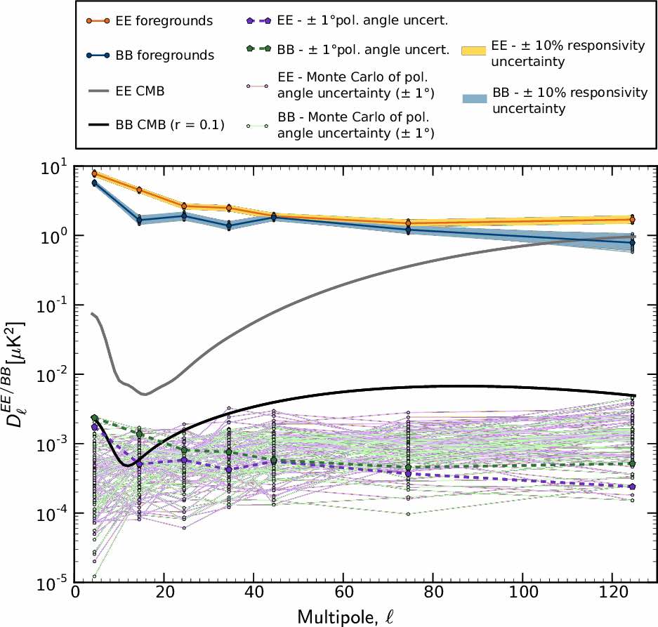
Figure 19: Power spectra evaluating the impact of polarization angle and photometric calibration uncertainty on Strip measurements.

4.2 LSPE-Strip calibration

We briefly describe here how we will measure the three main instrumental calibration parameters: (i) the photometric constant, (ii) the beam pattern and (iii) the polarization angle.

Photometric calibration.

We distinguish here two steps in the determination of the photometric constant: (i) “absolute calibration”, i.e. the determination of the absolute value of the photometric constant and, (ii) “relative calibration”, the measurement of time variations in the instrument responsivity caused by gain fluctuations.

Because the architecture of the Strip polarimeters does not allow stable measurements in total intensity, for absolute calibration we must rely on bright polarized sources with known flux. The Crab Nebula is undoubtedly the best flux calibrator at these frequencies and we have shown that with one day of data it is possible to achieve a precision $\lesssim 10\%$, while a few weeks will be enough to approach a precision of $2-3\%$ [106].

Regarding relative calibration, we will measure instrumental gain changes with a stable signal generated by two thermally stabilized microwave generators (one in Q-band and the other in W-band) installed in the optical assembly. Fluctuations currently measured in our laboratory are less than 0.2%, which will allow us to achieve a relative calibration with an overall precision better than 1%.

Beam calibration.

The presence of 1/$f$ noise in the total intensity data measured by Strip limits our ability to exploit natural point-sources, like Jupiter, to calibrate the main beams. Therefore, we have developed an artificial calibrator system based on a microwave source placed on an unmanned aerial vehicle (UAV) [107] that will fly over the Strip telescope during the commissioning campaign, and will allow us to measure the main beams with the required precision (1% at $-$25\text{\thinspace}\mathrm{d}\mathrm{B}$$).

Polarization angle.

The Strip polarimeters measure directly the Stokes parameters $Q$ and $U$ in a coordinate system defined by the mechanical layout of the polarizer-OMT assembly [46] and, ultimately, by the orientation of the OMT output waveguides. This means that the knowledge of the polarization angle is determined by the mechanical design and limited to about $0.5\text{\thinspace}\mathrm{\SIUnitSymbolDegree}$ by mechanical tolerances and by possible thermoelastic variations during cooldown.

4.3 LSPE-SWIPE systematic effects and calibration

The minimization and control of systematic effects is a critical aspect for instrumentation designed for measurement of the CMB B-mode polarization. In this section we discuss the main potential systematic effects in LSPE-SWIPE, we estimate their impact into the scientific target, and set the requirement on relevant instrumental parameters. Specifically, (i) in section 4.3.1 we set some basic requirements from unavoidable instrumental properties, order of magnitude estimation, and literature results; (ii) in section 4.3.2 we derive requirements for polarization angle and time response knowledge running the pixel-based tensor-to-scalar ratio estimation pipeline (detailed in section 5.2) for a coherent rotation of the polarization in the sky; (iii) in section 4.3.3 we derive requirements on the systematic effects produced by the HWP at the frequency of the plate rotation, and its harmonics, including a requirement on the knowledge of the HWP angular velocity and of the HWP angle, in terms of random error and systematic offset; this is obtained by a full end-to-end simulation of the LSPE-SWIPE observation, using the instrument simulator, prior of running the tensor-to-scalar ratio estimation pipeline; (iv) finally in section 4.3.4 we summarize the requirements and briefly describe the calibration philosophy.

4.3.1 LSPE-SWIPE optical parameters requirements

LSPE-SWIPE is designed to minimize instrumental polarization. This is the spurious signal resulting from the measurement of unpolarized radiation. In the case of CMB, the amount of unpolarized radiation coming from the sky is overwhelming with respect to the polarized signal, minimizing instrumental polarization is the most important driver of instrument design. In the case of SWIPE, some level of instrumental polarization is inevitably generated by the cryostat window, in case of incident radiation not orthogonal to the window surface itself. This is due to multiple reflections in an isotropic dielectric slab [108]. For the off-axis detectors, considering the physical properties of the thin window reported in section 3.2, this instrumental polarization will be up to 0.04%. Despite being a small value, it will produce a constant polarized signal at the level of $1\text{\thinspace}\mathrm{m}\mathrm{K}$ from the unpolarized CMB monopole, up to $2\text{\thinspace}\mathrm{\SIUnitSymbolMicro}\mathrm{K}$ spurious polarization from CMB dipole, and less than $25\text{\thinspace}\mathrm{n}\mathrm{K}$ from CMB anisotropy. The high constant signal is treated as an offset, removed in the data analysis. Its stability depends on the stability of the gain of the electronics and of the responsivity of the detectors and the effect of the instability is not synchronous with the observed sky. The detailed removal technique is described in section 4.3.3. Beyond this inevitable term, instrumental polarization is reduced by system design, with an optical system close to on-axis, avoiding mirrors in favor of lenses, and using the polarization modulator as the first optical element (except window and thermal filters), thus relaxing significantly the requirements on the following optical components.

The second parameter to be considered is cross-polarization, defined as the response of a polarimeter to an input signal polarized in direction orthogonal to the nominal polarimeter direction. Cross-polarization results in leakage of E-mode into B-mode. Our requirement is that the maximum acceptable level of cross-polarization is below 2%. This is achieved again by means of an accurate optical design, as described in section 2.3.5.

The third parameter to be considered is the ellipticity of the main beam (detector angular response in the sky). Spinning of the Half-Wave Plate allows the system to observe the same sky region with the same beam orientation, and different polarimeter orientation. This strongly mitigates the ellipticity requirement, which was tested with simulations up to 25% without a relevant impact, and differential ellipticity among different detectors.

Correct measurement of the angles of the polarimeters is crucial to avoid leakage from E-mode into B-mode, and to avoid contamination in the measurement of fundamental physics effects such as cosmic birefringence. In this context, our system is characterized by the presence of a single, large wire grid polarizer, defining the reference system for polarization measurements. With this design the system is similar to an ideal polarimeter, and the angle of the single large wire grid polarimeter can be accurately measured. The requirement on the polarimeter angle measurement is set in the next section.

Spectral matching among detectors has been historically a problem for instruments without a polarization modulator, just comparing two independent measurements of the orthogonal polarization components. In LSPE-SWIPE we use a Stokes polarimeter, where the same detector measures both polarizations, alternated by means of the rotating HWP. In this configuration the most important requirement is that the waveplate has high modulation efficiency over the detection bandwidth of the focal plane it serves. In our system a single waveplate covers all the bands from 120 to $260\text{\thinspace}\mathrm{G}\mathrm{H}\mathrm{z}$. This requires over 70% bandwidth for the waveplate, a goal certainly reachable with significant accuracy, by means of metamaterials [see 109].

Other relevant effects are the impact of polarized optical sidelobes, and the terms in the optical system Muller matrix converting radiation intensity into polarization. These effects are potentially critical for polarization estimation, even in presence of a HWP, and must be controlled by an effort in the calibration of the integrated system and in the data analysis. We note that simulations and data analysis of BICEP-2 [110] have shown that the polarized sidelobes induce a contamination at a level 400 times below the $r=0.1$ target, thus also below the target of LSPE-SWIPE which has a very similar shielding scheme. Regarding the spurious terms in the Mueller matrix, the critical elements are $M^{4\theta}_{IQ}$ and $M^{4\theta}_{IU}$ that induce a leakage modulated at $4\omega_{\text{HWP}}t$ in equation 2.1. It has been shown [111] that a 10^∘ tilted plate can induce these kind of terms at the level of $10^{-4}$, which contaminates the B-mode below the level relevant for LSPE-SWIPE; the Atacama B-mode Search (ABS) experiment [112] has measured intensity to polarization leakage of order $7\times 10^{-4}$, corresponding to a systematic error contribution of $r<0.01$, even without attempting to measure and remove the leakage signal [113]. It is also possible to measure some of these parameters, and compensate their effect adopting a mapmaking such as the one described in [114], which includes the spurious terms in the mapmaking equation. This approach requires a level of calibration of the intensity-to-polarization terms in the Mueller matrix terms $M_{IQ/U}^{4\theta}$ of the order of $10^{-4}$, which we set as a calibration requirement.

4.3.2 Polarization angle and detector time response requirements

One of most problematic systematic effects for any B-mode probe is the presence of a systematic error $\Delta\alpha$ in the polarization angle reconstruction. Such an error induces a $Q$ to $U$ rotation, and an E to B-mode leakage [115]:

$$\left\{\begin{aligned} C_{\ell}^{EE,obs}=C_{\ell}^{EE}\cos^{2}(2\Delta\alpha)+C_{\ell}^{BB}\sin^{2}(2\Delta\alpha)\\ C_{\ell}^{BB,obs}=C_{\ell}^{BB}\cos^{2}(2\Delta\alpha)+C_{\ell}^{EE}\sin^{2}(2\Delta\alpha).\end{aligned}\right.$$ (4.1)

In order to set the requirement on the knowledge of SWIPE wire grid and polarization angle, we have run an estimation of the likelihood of $r$, as described in section 5.2, for a sky with a rotation of the E, B space as in equation 4.1.

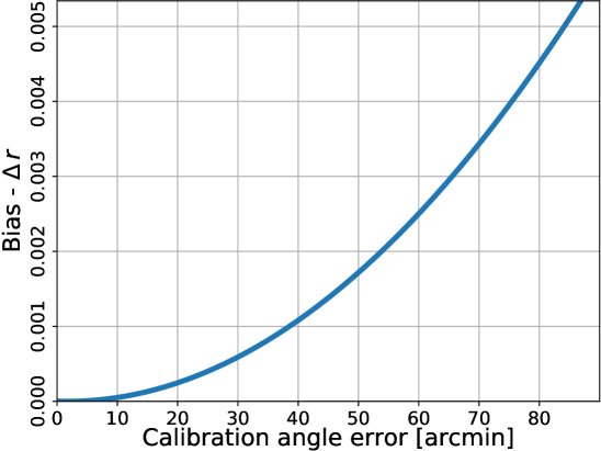
Figure 20: Bias in $r$ due to a rotation in the polarization angles. The bias is computed by adding a rotation to the polarization angles, and estimating the tensor-to-scalar ratio $r$ from pixel based likelihood as described in section 5.2.

The result is reported in figure 20, in terms of a bias in $r$, if the recovered polarization is rotated by a given angle. In the case of LSPE-SWIPE the rotation may be due to a rotation of the Wire Grid, by an angle $\Delta\phi_{\text{WG}}$ or by a rotation of the HWP, by an angle $2\Delta\theta_{\text{HWP}}$. From figure 20, we can set the requirements:

$$\Delta\phi_{\text{WG}}<$40\text{\thinspace}\mathrm{\SIUnitSymbolArcminute}$/\sqrt{2}=$28\text{\thinspace}\mathrm{\SIUnitSymbolArcminute}$$$ (4.2)

$$\Delta\theta_{\text{HWP}}<$20\text{\thinspace}\mathrm{\SIUnitSymbolArcminute}$/\sqrt{2}=$14\text{\thinspace}\mathrm{\SIUnitSymbolArcminute}$$$

so that the uncorrelated combination of the two errors is $\Delta\alpha=$40\text{\thinspace}\mathrm{\SIUnitSymbolArcminute}$$, which produces a bias $\Delta r\sim 0.001$, corresponding to 10% of the uncertainty in $r$. These requirements are valid for the angles’ knowledge, in the case that this is the only uncertainty in the system. In section 4.3.3 we consider the combination of a number of systematic effects, relevant for the measurement of the polarization. With that joint analysis, we set more stringent requirements as reported in table 6.

The TES detectors of SWIPE have an intrinsic time response. Their temporal transfer function $H(\omega)$ can be approximated by a single pole low pass filter, as in equation A.1. As described in appendix D, an error in the knowledge of the temporal transfer function phase has the same effect of an error on the knowledge of the HWP angle. The requirements on transfer function phase and the time constant knowledge can then be derived from the requirement on the angles reconstruction. In appendix D, we derive:

$$\Delta\Phi\simeq$42\text{\thinspace}\mathrm{\SIUnitSymbolArcminute}$=12\times 10^{-3}\thinspace\text{rad}$$

$$\Delta\tau_{\text{LP}}\simeq$1.5\text{\thinspace}\mathrm{m}\mathrm{s}$$$

where $\Delta\Phi$ is the error in the knowledge of the temporal transfer function phase in the range $[3\div 5]\omega_{\text{HWP}}$, and $\Delta\tau_{\text{LP}}$ is the corresponding error in the knowledge of the detector’s time constant; Also in this case, the requirement will be more stringent if considered jointly with other effects, as presented in table 6. The HWP angle error and the error on the phase of the time transfer function can be disentangled and calibrated by spinning the HWP at different angular velocities, or different directions, both in flight and during ground calibration.

4.3.3 HWP synchronous systematic effects: mitigation and requirements

Besides errors in the polarization angle reconstruction, discussed in the previous section, another critical contamination in HWP based polarimeters is the generation of spurious signals at the frequency of the plate rotation, or its harmonics. Small differences ($\sim 10^{-3}$) in the absorption coefficients along the ordinary and extraordinary axes of the HWP produce a polarized emission. This radiation is modulated at twice the HWP spin frequency, $2f_{\text{HWP}}$, when it is transmitted by the polarizer but could also be reflected by the polarizer, and back by the HWP, and induce a spurious signal at $4f_{\text{HWP}}$, the same frequency as the sky polarized signal [116]. By simulations, the $2f_{\text{HWP}}$ contribution produces an equivalent temperature fluctuation of $\sim 1-$10\text{\thinspace}\mathrm{m}\mathrm{K}_{CMB}$$ while the $4f_{\text{HWP}}$ contribution is $<$5\text{\thinspace}\mathrm{\SIUnitSymbolMicro}\mathrm{K}_{CMB}$$ if the HWP temperature is kept below $10\text{\thinspace}\mathrm{K}$. This last term is completely negligible in comparison to the instrumental polarization requirement set at 0.04%, corresponding to a polarization signal of $1\text{\thinspace}\mathrm{m}\mathrm{K}$. These spurious signals must be removed by dedicated data analysis techniques. For the case of SWIPE, we developed a specific pipeline to deal with any spurious term synchronous with the HWP spin frequency and harmonics. This is based on application of notch filters, centered at the contaminated frequencies, and an iterative map-making to recover the removed signal, as described in Appendix E. In order to assess the efficacy of this technique, we performed a set of simulations, using a multi-notch filter, i.e. a chain of notch filters, each with different central frequency. The payload rotation period is set to $8.6\text{\thinspace}\mathrm{m}\mathrm{i}\mathrm{n}$ in accordance with equation A.2 and the notch filters width is set to $\Delta f=$1\text{\thinspace}\mathrm{m}\mathrm{H}\mathrm{z}$$. HWP synchronous systematic effects are introduced at $\text{1}f_{\text{HWP}}$, $\text{2}f_{\text{HWP}}$,$\text{3}f_{\text{HWP}}$, $\text{4}f_{\text{HWP}}$ and $\text{5}f_{\text{HWP}}$ with amplitude $10\text{\thinspace}\mathrm{m}\mathrm{K}$, $10\text{\thinspace}\mathrm{m}\mathrm{K}$, $1\text{\thinspace}\mathrm{m}\mathrm{K}$, $1\text{\thinspace}\mathrm{m}\mathrm{K}$ and $1\text{\thinspace}\mathrm{m}\mathrm{K}$ respectively. The same frequencies are used as centers of a stack of 5 notch filters. Notably, the application of these 5 notch filters and the iterative map-making impact the polarization map with a r.m.s of the residual map of order $5\text{\times}{10}^{-12}\text{\thinspace}\mathrm{K}_{CMB}$, showing that the procedure has unitary transfer function at all angular scales.

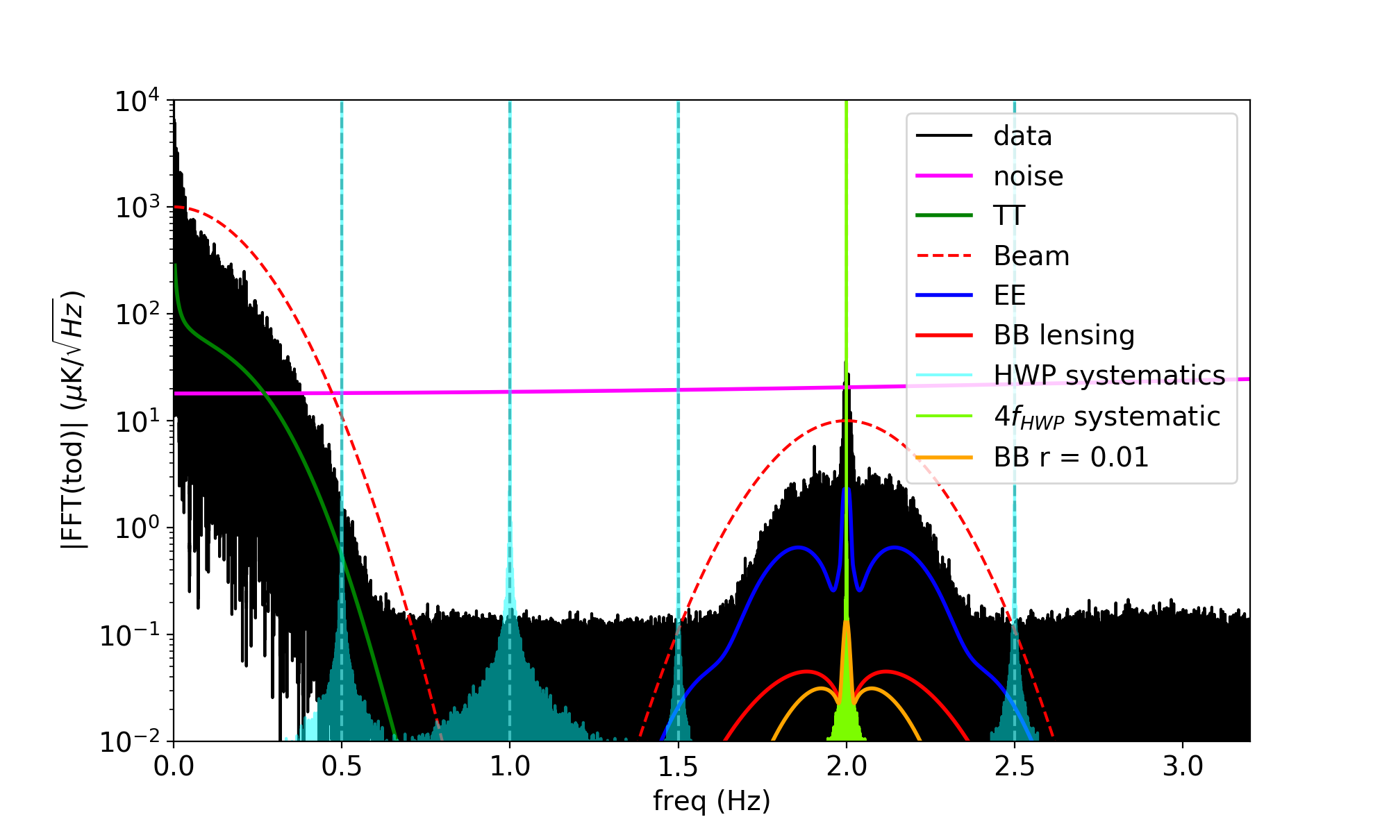
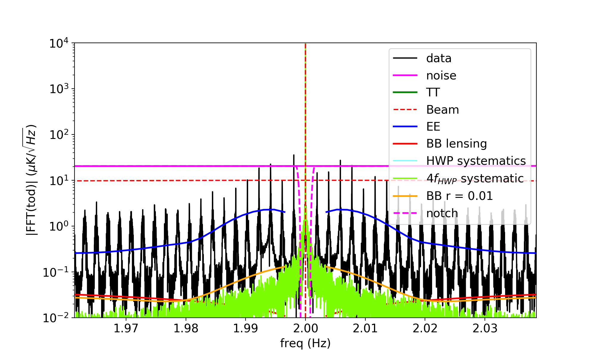
Figure 21: LSPE-SWIPE frequency spectrum (top), and zoom-in near modulation frequency (bottom), for a 16 hours noise-free CMB-only simulated timestream. The black curve represents the data; CMB temperature data are centered around 0 frequency, and polarization data around $4f_{\text{HWP}}$. The magenta line is the noise for a single detector at $145\text{\thinspace}\mathrm{G}\mathrm{H}\mathrm{z}$. The magenta dashed line, is the noise multiplied by the notch filter. Vertical dashed lines represent harmonics of the HWP spin frequency. The dark green curve is the expected signal for a temperature CMB angular power spectrum, blue curve for E-mode power spectrum, red for B-mode ( lensing only) and orange for inflationary B-mode. The light-green curve, visible in the bottom plot, is a systematic effect at $4f_{\text{HWP}}$, with an amplitude of $1\text{\thinspace}\mathrm{m}\mathrm{K}$, spread in frequency due to the uncertainty in the HWP angular velocity $\sigma_{\omega_{\text{HWP}}}/\omega_{\text{HWP}}=0.6\times 10^{-6}$. The cyan clear curves are the systematic effects at 1, 2, 3, 5$f_{\text{HWP}}$, as discussed in section 4.3.3. Since the signal is quasi-periodic, with period $T_{\text{payload}}$, its Fourier transform peaks at the modulation frequency $4f_{\text{HWP}}$ and then in frequency shifts equal to $\Delta f=1/T_{\text{payload}}$, clearly visible in the bottom figure.

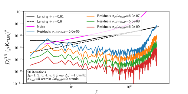
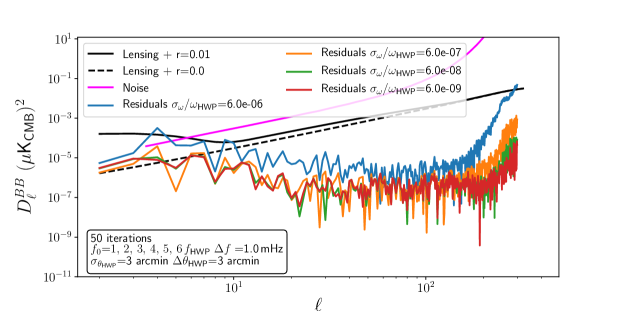
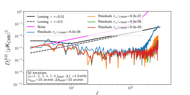
Figure 22: Impact of HWP synchronous systematic effects at $\text{1}f_{\text{HWP}}$, $\text{2}f_{\text{HWP}}$, $\text{3}f_{\text{HWP}}$, $\text{4}f_{\text{HWP}}$ and $\text{5}f_{\text{HWP}}$, with amplitude $10\text{\thinspace}\mathrm{m}\mathrm{K}$, $10\text{\thinspace}\mathrm{m}\mathrm{K}$, $1\text{\thinspace}\mathrm{m}\mathrm{K}$, $1\text{\thinspace}\mathrm{m}\mathrm{K}$, and $1\text{\thinspace}\mathrm{m}\mathrm{K}$ respectively. Black lines: B-mode angular power spectra for $r=0$ (dashed) and $r=0.01$ (continuous). Coloured lines: residual of B-mode power spectra of simulated map with HWP synchronous systematic effects and notch filters, with respect to simulated map without systematic effects nor filters. The three panels are for the cases: (top) with HWP synchronous systematic effects, and HWP instability; (mid) with HWP synchronous systematic effects, HWP instability, $\Delta\theta_{\text{HWP}}=$3\text{\thinspace}\mathrm{\SIUnitSymbolArcminute}$$ and $\sigma_{\theta_{\text{HWP}}}=$3\text{\thinspace}\mathrm{\SIUnitSymbolArcminute}$$; (bottom) with HWP synchronous systematic effects, HWP instability, $\Delta\theta_{\text{HWP}}=$10\text{\thinspace}\mathrm{\SIUnitSymbolArcminute}$$ and $\sigma_{\theta_{\text{HWP}}}=$10\text{\thinspace}\mathrm{\SIUnitSymbolArcminute}$$; in all panels, there are 4 continuous lines, corresponding to different levels of HWP instability with angular speed uncertainty: $\sigma_{\omega_{\text{HWP}}}/\omega_{\text{HWP}}=[0.6\times 10^{-8},0.6\times 10^{-7},0.6\times 10^{-6},0.6\times 10^{-5}]$. The magenta line is the noise power spectrum after component separation.

In order to have a more realistic simulation, this contamination has been combined with:

• an error in the measurement of the HWP angle. This is defined by the uncertainty with which we can readout the HWP angle. This is described by the parameter $\sigma_{\theta_{\text{HWP}}}$. We have explored $\sigma_{\theta_{\text{HWP}}}=[0,3,10]~{}$\text{\thinspace}\mathrm{\SIUnitSymbolArcminute}$$. Our measurement precision, with Kalman filter approach , is of order $\sigma_{\theta_{\text{HWP}}}\leq$0.1\text{\thinspace}\mathrm{\SIUnitSymbolArcminute}$$;

• an offset in the knowledge of the HWP angle. This is described by the parameter $\Delta\theta_{\text{HWP}}$. We explored the values $\Delta\theta_{\text{HWP}}=[0,3,10]~{}$\text{\thinspace}\mathrm{\SIUnitSymbolArcminute}$$;

• an instability in the HWP rotation rate, modeled as a noise in the angular velocity of the HWP. This is described in terms of relative error by the parameter $\sigma_{\omega_{\text{HWP}}}/\omega_{\text{HWP}}$. The angular velocity samples are simulated as

  $$\omega_{i}=\omega_{HWP}\left(1+\frac{\sigma_{\omega_{\text{HWP}}}}{\omega_{\text{HWP}}}n_{i}\sqrt{\frac{f_{\text{sampling}}}{f_{\text{HWP}}/\text{dpr}}}\right)$$ (4.3)

  where $n_{i}$ is a sample of a normal distributed random number, $f_{\text{sampling}}$ is the simulation sampling rate (100 Hz in our case), $f_{\text{HWP}}$ is the HWP rotation frequency, and ${\rm dpr}=64$ is the number of angle measurements of the HWP in a revolution. The ratio $f_{\text{sampling}}/(f_{\text{HWP}}/\text{dpr})$ corresponds to the number of simulated samples between two subsequent HWP measured positions (data per revolution). The simulation with equation 4.3 results in the same angular drift between two HWP angle measurements, independently of the sampling rate of the simulation. We explored the values $\sigma_{\omega_{\text{HWP}}}/\omega_{\text{HWP}}=[0,0.6\times 10^{-8},0.6\times 10^{-7},0.6\times 10^{-6},0.6\times 10^{-5}]$. Using the Kalman filter approach, we have measured a precision in the determination of the HWP angular velocity of order $\sigma_{\omega_{\text{HWP}}}/\omega_{\text{HWP}}=2\times 10^{-6}$.

The major contribution from HWP spin rate instability is due to the fact that the various HWP synchronous effects are not at a single frequency anymore, but are spread in frequency due to the instability, thus reducing the efficacy of the notch filter; this is partially compensated by measuring this instability, and filtering in the angle domain instead of the time domain, but with some limitation coming from the uncertainty in the angular velocity measure, $\sigma_{\omega_{\text{HWP}}}/\omega_{\text{HWP}}$.

Figure 21 illustrates the LSPE-SWIPE frequency spectrum of a $16\text{\thinspace}\mathrm{h}\mathrm{r}\mathrm{s}$ noise-free timeline, for simulations of CMB and systematic effects (see caption for details). Figure 22 presents the results of this analysis in terms of B-mode angular power spectra. The black lines are the B-mode angular power spectra in case of $r=0$ and $r=0.01$, which is the limit of our sensitivity. The coloured lines represent the residual power spectra of the case with systematic effects and notch filter, versus the ideal case, without systematic effects nor filters. Notably, in this figure we consider a combination of several systematic effects: instrumental polarization, HWP angle errors, HWP angle offset, uncertainty in the measurement of the HWP angular velocity. Applying the $r$ estimation pipeline (see section 5.2) to the maps contaminated by the combinations of systematic effects just described, we obtain a bias in $r$ as reported in figure 23. The maps used to produce values in this figure are simulated with $\sigma_{\theta_{\text{HWP}}}=$10\text{\thinspace}\mathrm{\SIUnitSymbolArcminute}$$; $\Delta\theta_{\text{HWP}}=$10\text{\thinspace}\mathrm{\SIUnitSymbolArcminute}$$; synchronous systematic effects at [1,2,3,4,5] $f_{\text{HWP}}$ with amplitude [10,10,1,1,1] $\text{\thinspace}\mathrm{m}\mathrm{K}$ respectively; and $\sigma_{\omega}/\omega_{\text{HWP}}$ as in the abscissas.

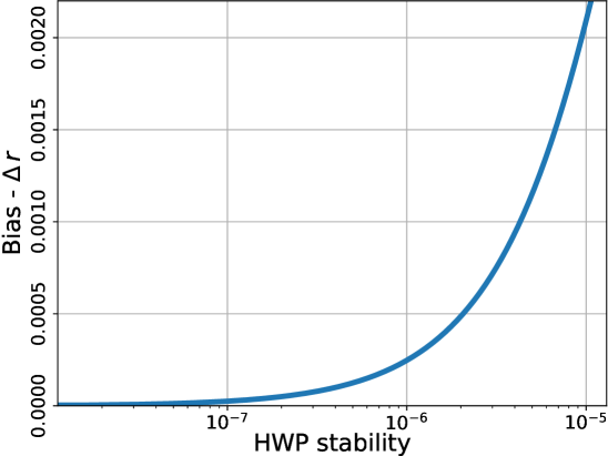
Figure 23: Bias in $r$ due to instability of the HWP, combined with instrumental polarization, HWP angle offset, and HWP angle measurement error.

4.3.4 LSPE-SWIPE calibration

From the analysis reported in section 4.3 and subsections, we set the requirements reported in table 6, for the most critical systematic effects for LSPE-SWIPE polarization measurement, considered jointly. In the table the B-mode r.m.s contamination is computed from the r.m.s. of the anisotropy (for intensity to polarization leakage) or from the r.m.s. of the E-mode (for the E- to B-mode leakage) multiplied by the leakage factor. The r.m.s. is computed from the angular power spectrum as

$$\sqrt{\langle\Delta T^{2}\rangle}=\sqrt{\frac{1}{4\pi}\sum(2\ell+1)C_{\ell}B_{\ell}^{2}}$$

The r.m.s values reported in the table are computed for a uniform systematic effect on the full focal plane. In practice each detector will have a different effect, and for some of the systematic effects cancelations will occur due to redundancy. On the mission data, the impact of the residual systematic effects will be assessed by estimation of the bias in the angular power spectra, by means of end-to-end Monte Carlo simulations.

LSPE-SWIPE Parameter	Requirement	B-mode	reference
		(r.m.s.)
Instrumental polarization1,2	$<4\times 10^{-4}$	18 nK${}_{\text{CMB}}$	4.3.1
Cross polarization2	$<0.02$	10 nK${}_{\text{CMB}}$	4.3.1
Polarization angle recovery	$<$40\text{\thinspace}\mathrm{\SIUnitSymbolArcminute}$$	12 nK${}_{\text{CMB}}$	4.3.2
WG angle error	$\Delta\phi_{\text{WG}}<$20\text{\thinspace}\mathrm{\SIUnitSymbolArcminute}$$	6 nK${}_{\text{CMB}}$	4.3.2, 4.3.3
HWP angle offset	$\Delta\theta_{\text{HWP}}<$10\text{\thinspace}\mathrm{\SIUnitSymbolArcminute}$$	6 nK${}_{\text{CMB}}$	4.3.2, 4.3.3
HWP angle noise	$\sigma_{\theta_{\text{HWP}}}<$10\text{\thinspace}\mathrm{\SIUnitSymbolArcminute}$$	6 nK${}_{\text{CMB}}$	4.3.2, 4.3.3
Time constant knowledge2	$\Delta{\tau_{\text{LP}}}<$1.0\text{\thinspace}\mathrm{m}\mathrm{s}$$	6 nK${}_{\text{CMB}}$	4.3.2, 4.3.3
HWP angular velocity measurement	$\sigma_{\omega_{\text{HWP}}}/\omega_{\text{HWP}}<5\times 10^{-6}$	6 nK${}_{\text{CMB}}$	4.3.3
Mueller matrix $I\rightarrow Q/U$ terms knowledge	$\Delta{M^{4\theta}_{IQ}},\Delta{M^{4\theta}_{IU}}<10^{-4}$	6 nK${}_{\text{CMB}}$	[111, 112]
1 This is an inevitable term given by the effect of the radiation crossing the cryostat window with a tilted angle, and is so large only for the most off-axis detectors. The equivalent B-mode r.m.s. value is obtained multiplying the CMB anisotropy r.m.s by the coefficient, divided by $\sqrt{2}$, assuming equal E-, B-mode distribution.
2 The r.m.s. contribution is for a single detector and is not expected to be correlated among detectors. The impact will be reduced due to redundancy and cancelations.

Table 6: LSPE-SWIPE main systematic effects and calibration requirements. These requirements are derived considered the various effects jointly. $\Delta$-s represent maximum offsets between true and measured values, $\sigma$-s represent fluctuations between the true values and the measured ones. The B-mode r.m.s. contamination is computed from leakage of intensity or E-mode r.m.s into B-mode. This is only an order of magnitude estimation of the real impact into $r$ estimation, given that the real contamination depends on the distribution of the leakage in the B-mode angular power spectrum. Some of these results are derived by a order of magnitude analysis in section 4.3.1, some from literature papers, while the most critically related to the use of the HWP are derived from the simulations described in sections 4.3.2 and 4.3.3 (see the reference column).

As in the case of Strip, the SWIPE calibration will be performed in multiple stages:

1. at sub-system level: components will be tested individually in order to define specific properties. These components include optical filters, HWP, horns, detectors, readout electronics;

2. at system level: the integrated system, will undergo a long list of calibration tests on the ground. These include test of the polarization properties of the integrated system as a function of frequency, band-integrated polarization properties, angle dependent polarization properties, band-pass definition, angular response (by means of a far field thermal source). It is worth noting that the properties of the instrument are not expected to change from ground to the stratosphere, given that the thermal configuration is the same; the major change will be in the different background which is expected to modify the detector responsivity, to be confirmed in flight;

3. during observation: the payload will undergo a limited number of tests for verification of the ground-based calibration parameters. In particular, these tests will be updating detector responsivity, updating the pointing direction of each detector with respect to the telescope reference frame, and confirming polarization properties of the system, by observation of the Crab nebula [117], and by minimization of the E-B modes correlation.

5 Results

In this section we describe the component separation and the likelihood methods, and we forecast the main results of LSPE in terms of cosmological parameters. It is assumed that the systematic effects are within the requirements defined in section 4. In each of the maps the noise is estimated using the NETs from tables 2 and 4, projected into maps by means of the instrument simulators described in appendix B.

5.1 Component separation

Component separation is a key element in CMB data analysis, and it turns out to be particularly challenging for the extraction of CMB polarization (see e.g. [118, 119, 120]). In particular, diffuse Galactic dust and synchrotron emissions are the most relevant foregrounds in polarization. For the analysis presented in this paper, we consider the component separation apparatus represented by the ForeGroundBuster, which is currently used to assess the foreground cleaning capabilities of a number of CMB B-mode probes [121, 122]. The method fits, in each pixel observed by both Strip and SWIPE, for CMB signal, amplitude and spectral index of synchrotron, temperature, amplitude and spectral index of dust. In our analysis, we include thermal dust and synchrotron as polarized foregrounds. We exploit the publicly available package Python Sky Model (PySM) which generates full sky simulated foregrounds in intensity and polarization, and consider the d0s0 configuration outlined below [123]. The synchrotron spectral brightness is modeled as a power law in frequency with a constant spectral index $\beta_{s}=-3$: $I_{s}(\nu,\hat{n})=A_{s}(\hat{n})(\nu/\nu_{0})^{\beta_{s}}$, where $A_{s}(\hat{n})$ is the synchrotron amplitude. The dust component is modeled as a grey body, i.e. an almost thermal component at a temperature of $T_{d}=20$ K, heated back by starlight which is represented as an emissivity factor scaling as a power law in frequency, with spectral index $\beta_{d}=1.54$: $I_{d}(\nu,\hat{n})=\tau_{0}(\hat{n})(\nu/\nu_{0})^{\beta_{d}}B(\nu,T_{d})$. The component separation procedure is performed only in polarization and recovers the value of the spectral indices $\beta_{s},\beta_{d}$ which are not varying in the sky, as well as the amplitude of the synchrotron signal $A_{s}(\hat{n})$ and dust optical depth $\tau_{0}(\hat{n})$, which vary with the sky direction. The assumption of uniform spectral indices could lead to biases on the estimation of the tensor-to-scalar ratio. This is true, in particular, for experiments targeting $r\simeq 10^{-3}$, for which the estimation of the foreground parameters must be done in the various regions of the sky independently. For experiments targeting higher values of $r$, such as LSPE, the impact of this spatial variation is expected to be less dramatic, leading to a bias lower than or comparable to the statistical uncertainties. This result is confirmed by the SO paper [16], section 3.4.2, in particular in Table 4, where the first row of the table reports the case of fitting a sky model built with varying spectral indices, assuming uniform spectral indices in the reconstruction. This results in a bias in $r$ of order $\Delta r\simeq 2\times 10^{-3}$.

In addition to the LSPE bands, we also consider the observations of the Planck satellite between 30 and $353\text{\thinspace}\mathrm{G}\mathrm{H}\mathrm{z}$ [3], and the ones of QUIJOTE at $11\text{\thinspace}\mathrm{G}\mathrm{H}\mathrm{z}$ [38, 124]. At each of the frequencies corresponding to these probes, and separately for the $Q$ and $U$ Stokes parameters, we generate and add foregrounds and CMB using the PySM, and also add noise realizations according to the SWIPE, Strip, Planck and QUIJOTE sensitivities. We convolve all maps with a Gaussian beam in order to reach a common $85\text{\thinspace}\mathrm{a}\mathrm{r}\mathrm{c}\mathrm{m}\mathrm{i}\mathrm{n}$ FWHM, which corresponds to the largest beam associated to the LSPE channels. All maps are generated using HEALPix at $N_{\text{side}}=128$. We did not consider any pixel-pixel correlation property of the noise. The data model which is implemented in ForeGroundBuster and used in this paper is $d(\nu)\equiv\mathsf{A}s+n$, where $d(\nu)$ contains measured signal at each frequency $\nu$, $s$ are the maps of the different components, $\mathsf{A}$ is the mixing matrix which contains the parametric model to fit, and $n$ represents the noise in the maps. The parametric component separation process consists in obtaining an estimate $\tilde{s}=\mathsf{W}d$ of the components, by means of a kernel operator $\mathsf{W}$. Therefore, the key element of component separation is the $\mathsf{W}$ matrix, which is the linear operator that mixes the frequency maps in the component maps, taking into account the sensitivity and the contribution of each frequency to each astrophysical component. The elements $W_{i,j}$ of the $\mathsf{W}$ matrix (often referred as weights) admit negative values for frequencies that must be subtracted in order to solve for the astrophysical component. Frequency bands and weights for each component are shown in table 7.

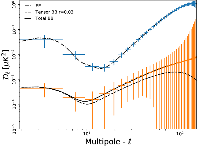
Figure 24: CMB E-mode (blue) and B-mode (orange) power spectra averaged over 1000 simulations after Component separation in the baseline case of table 7.

From this table it is clear that the 145 GHz channel is the most important one for reconstructing the CMB, clearly adding sensitivity to the currently available datasets. The table also quantitatively shows relevance of higher and lower frequency bands for fitting and subtracting foregrounds. As an illustration, figure 24 shows the polarization CMB power spectra [125] obtained averaging 1000 simulations after component separation.

In table 8, we show a minimal case, where we have used just the $30\text{\thinspace}\mathrm{G}\mathrm{H}\mathrm{z}$ channel of Planck and LSPE frequencies. Moreover, table 9 shows the accuracy of the component separation in terms of dust and synchrotron spectral indices.

Band (GHz)	Probes	wCMB $\scriptstyle\times 10^{3}$	wDust $\scriptstyle\times 10^{3}$	wSynch $\scriptstyle\times 10^{3}$
11	QUIJOTE	$-$1.1	0.24	56
30	Planck	2.5	$-$1.1	18
43	Strip	4.4	$-$1.9	8.0
44	Planck	1.9	$-$0.82	3.2
70	Planck	2.8	$-$1.1	0.86
100	Planck	14	$-$5.3	0.41
143	Planck	26	$-$7.4	$-$2.2
145	SWIPE	1200	$-$330	$-$110
210	SWIPE	$-$130	200	5.6
217	Planck	$-$7.1	8.5	0.48
240	SWIPE	$-$150	130	14
353	Planck	$-$9.9	6.5	1.2

Table 7: Component separation weights for each component in each channel.

Band (GHz)	Probes	wCMB $\scriptstyle\times 10^{3}$	wDust $\scriptstyle\times 10^{3}$	wSynch $\scriptstyle\times 10^{3}$
30	Planck	$-$15	2.7	870
43	Strip	$-$2.6	$-$0.45	390
145	SWIPE	1400	$-$410	$-$1600
210	SWIPE	$-$190	240	28
240	SWIPE	$-$200	160	340

Table 8: Component separation weights for each component in each channel.

Parameter	Mean	$\sigma$
$\beta_{d}$	1.539	0.001
$\beta_{s}$	$-$2.999	0.002

Table 9: Dust and synchrotron spectral indices obtained by parametric component separation. The component separation algorithm fits for a single value in each map. The uncertainties are derived from the standard deviation of 1000 realizations of the noise in the maps.

5.2 Likelihood

The likelihood used in the parameter estimation is based on maps of Stokes parameters $T,Q,U$ in HEALPix format. For the temperature map we assume perfect component separation outside a Galactic masks with $2\text{\thinspace}\mathrm{\SIUnitSymbolMicro}\mathrm{K}$ per pixel of white noise. The polarization maps after the component separation procedure, described in the previous section, are modeled as a sum of CMB signal, instrumental Gaussian noise and foreground Gaussian residuals. This modeling is consistent with analyses performed on current data at large angular scales [126] and with forecasts performed on other forthcoming data [16]. In this scenario the full likelihood expression reads

$$\mathcal{P}(\vec{m}|C_{\ell})=\frac{1}{2\pi|\mathsf{C}(C_{\ell})|^{1/2}}\exp\left(-\frac{1}{2}\vec{m}^{\mathsf{T}}\thinspace\left[\mathsf{C}(C_{\ell})\right]^{-1}\vec{m}\right)\thinspace,$$ (5.1)

where $\vec{m}\equiv{T,Q,U}$ is the data vector and $\mathsf{C}$ is total covariance matrix defined as the sum of signal and noise parts as

$$\mathsf{C}(C_{\ell})=\sum_{\ell=2}^{\ell_{\rm max}}\sum_{XY}\frac{2\ell+1}{4\pi}\thinspace B_{\ell}^{2}C_{\ell}^{XY}\mathsf{P}_{\ell}^{XY}+\mathsf{N},$$ (5.2)

here $B_{\ell}$ is the beam window function, $\mathsf{P}_{\ell}^{XY}$ are the associated Legendre polynomials, as defined in [127], and $\mathsf{N}$ is the pixel-pixel noise covariance matrix.

In order to speed up the computation we perform the likelihood evaluation on lower resolution maps, still able to keep the full potentiality of LSPE maps. We consider two resolutions, HEALPix $N_{\mathrm{side}}=16$ ($\ell_{\text{max}}=32$), with a Gaussian beam of $\text{FWHM}=$440\text{\thinspace}\mathrm{\SIUnitSymbolArcminute}$$, which allows us to measure the E-mode reionization peak used for optical depth $\tau$ estimation in section 5.3, and HEALPix $N_{\mathrm{side}}=64$ ($\ell_{\text{max}}=128$), with a Gaussian beam of $\text{FWHM}=$110\text{\thinspace}\mathrm{\SIUnitSymbolArcminute}$$, capable of measuring both the reionization and recombination peaks of the B-mode spectrum, used for tensor-to-scalar ratio $r$ and cosmic birefringence estimation in sections 5.4 and 5.5.

The likelihood analysis is performed simultaneously on a Monte Carlo of 1000 CMB, noise and residual foreground realizations. For each realization we estimate the reionization optical depth $\tau$ and the tensor-to-scalar ratio $r$. For each instrumental configuration the LSPE uncertainty on $\tau$ and $r$ is computed taking the average over the 1000 realizations of the $\log\left(\mathcal{P}(\vec{m}|C_{\ell})\right)$. In this way we efficiently take care of the scatter due to cosmic variance and instrumental noise. The other $\Lambda$CDM parameters are not sampled in this analysis, nonetheless we verified that opening the parameter exploration to full $\Lambda$CDM, and including a high-$\ell$ likelihood with noise performance compatible with Planck, provides equivalent results.

5.3 Reionization optical depth constraints

Measuring the polarization at very large scales, in particular the so-called reionization bump, allows constraining the Thompson scattering optical depth $\tau$. LSPE provides a cosmic variance limited measure of the polarization signal at very large scales ($\ell\mathrel{\raise 1.72218pt\hbox{\hbox to0.0pt{$<$\hss}\lower 5.16663pt\hbox{$\sim$}}}20$) on $\sim 35\%$ of the sky. For the analysis presented here we conservatively consider a smaller portion, $f_{\rm sky,cmb}\simeq 25\%$, removing regions close to the Galactic plane potentially contaminated by residual foregrounds. The LSPE sensitivity over such a sky fraction overcomes the current best estimates provided by Planck HFI, i.e. $\tau=0.059\pm 0.006$ [128], reaching $1-\sigma$ error on $\tau$ of $\sim 0.004$.

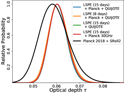
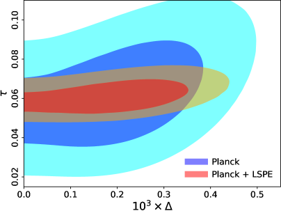
Figure 25: Left: posterior probability for optical depth $\tau$. The colored lines show different component separation configurations, see text for details. The black line shows the current best estimate on $\tau$. Right: Joint posterior probability for scale parameter $\Delta$ in ($\text{\thinspace}\mathrm{M}\mathrm{p}\mathrm{c}^{-1}$) and optical depth $\tau$. Blue and cyan are 68% and 95% CL for Planck; red and orange for Planck and LSPE.

The constraints on the reionization optical depth $\tau$ are reported in table 10 and figure 25 for different data combinations. For Strip we consider $2\text{\thinspace}\mathrm{y}\mathrm{e}\mathrm{a}\mathrm{r}\mathrm{s}$ of observations, for SWIPE we explore two possibilities, $15\text{\thinspace}\mathrm{d}\mathrm{a}\mathrm{y}\mathrm{s}$ (SWIPE 15) or $8\text{\thinspace}\mathrm{d}\mathrm{a}\mathrm{y}\mathrm{s}$ of observation (SWIPE 8). Planck and QUIJOTE are assumed with their nominal observational strategies and only considered in the portion of sky in common with LSPE. The $\tau$ constraints are rather stable showing that even after 8 days of SWIPE observations we reach the mission goal. Furthermore, even in a minimal configuration which considers only LSPE plus Planck $30\text{\thinspace}\mathrm{G}\mathrm{H}\mathrm{z}$ as additional synchrotron tracer, the $\tau$ measure does not change substantially, showing that we are not heavily dependent on the usage of external datasets.

Data Combination	$\sigma_{\tau}$
Strip + SWIPE 15 + QUIJOTE + Planck	0.0037
Strip + SWIPE   8 + QUIJOTE + Planck	0.0040
Strip + SWIPE 15 + QUIJOTE	0.0038
Strip + SWIPE 15 + Planck 30GHz	0.0038

Table 10: Forecasted $1-\sigma$ errors on $\tau$ for different data combinations obtained by marginalizing over $\ln(10^{10}A_{\rm s})$. SWIPE 15 and SWIPE   8 stand respectively for 15 and $8\text{\thinspace}\mathrm{d}\mathrm{a}\mathrm{y}\mathrm{s}$ of mission time, in both cases the effective time used for the sky survey is reduced by $1\text{\thinspace}\mathrm{d}\mathrm{a}\mathrm{y}$ used for calibration and ancillary operations.

LSPE can also provide valuable information on the study of one of the most discussed anomalies related to CMB, i.e. the lack of power at large angular scales in the anisotropy power spectrum [129, 130, 131, 132, 133]. Entering in details about modeling and possible constraining techniques is beyond the scope of this paper. Here we only want to show how, in the context of a specific model such as the one predicting early departure from slow-roll inflation [see e.g. 134, 135], LSPE provides valuable constraints, being able to break completely the remaining degeneracy that such models still have with the reionization optical depth $\tau$ in the current CMB data [136, 137]. As an example, the model described in [138] modifies the primordial scalar power spectrum according to:

$$P_{\Delta}(k)=A_{s}\frac{\left(k/k_{*}\right)^{3}}{\left[\left(k/k_{*}\right)^{2}+\left(\Delta/k_{*}\right)^{2}\right]^{2-\frac{n_{s}}{2}}},$$

where $k$ is the primordial perturbation wavenumber in $\text{\thinspace}\mathrm{M}\mathrm{p}\mathrm{c}^{-1}$, $A_{s}$ and $n_{s}$ are respectively the amplitude and the tilt of scalar perturbations, $k_{*}=$0.05\text{\thinspace}\mathrm{M}\mathrm{p}\mathrm{c}^{-1}$$ is the pivot scale, and $\Delta$ is a characteristic scale which breaks the power-law at very low wavenumbers damping both temperature and polarization power spectra at low multipoles. In this particular case, as shown in right panel of figure 25, LSPE improves the Planck constraint, substantially canceling the degeneracy with $\tau$.

5.4 Tensor-to-scalar ratio constraints

The angular resolution of LSPE and the observational strategy allow measuring simultaneously both the reionization and the recombination peaks of the primordial B-mode spectrum. This makes LSPE an extremely complete and unique instrument observing a region of the sky not entirely visible from the southern hemisphere. Nevertheless the relatively small sky fraction usable, if compared with a satellite mission, limits our sensitivity at very large scales. In table 11 we report the constraints on $r$ for the different data combinations; two input $r$ values have been considered, i.e., $r=0.03$ and $r=0$. The aggregate sensitivity allows detecting $r=0.03$ with $3-\sigma$ significance for different data combinations. In this case limiting the mission time of SWIPE to $8\text{\thinspace}\mathrm{d}\mathrm{a}\mathrm{y}\mathrm{s}$ induces a non-negligible effect, reducing the $r$ significance down to $\sim 2.3\thinspace\sigma$, still within the mission requirements. In the case of no primordial B-mode, the combination of Strip and SWIPE with both Planck and QUIJOTE as foreground tracers sets an upper limit $r<0.015$ at 95% confidence level ($r<0.024$ in the case of $8\text{\thinspace}\mathrm{d}\mathrm{a}\mathrm{y}\mathrm{s}$ of SWIPE observations).

Data Combination	$\sigma_{\rm r}$	95%cl
Strip + SWIPE 15 + QUIJOTE + Planck	0.0093	0.015
Strip + SWIPE   8 + QUIJOTE + Planck	0.013	0.024
Strip + SWIPE 15 + QUIJOTE	0.0098	0.016
Strip + SWIPE 15 + Planck 30GHz	0.010	0.018

Table 11: Expected sensitivity on the tensor-to-scalar ratio $r$. The second column shows $1-\sigma$ errors assuming an input $r=0.03$. The third column shows $95\%$ c.l. upper limits assuming no tensor B-modes (i.e. $r=0$).

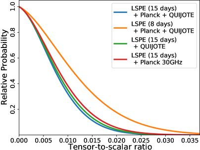
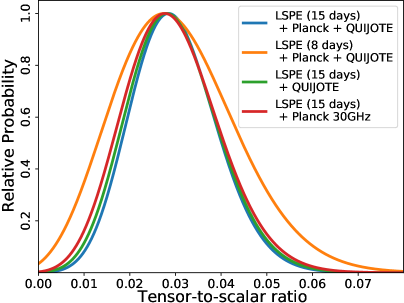
Figure 26: Posterior probability for tensor-to-scalar ratio $r$ in case of $r=0$ (left) and $r=0.03$ (right). The colored lines show different component separation configurations, see text for details.

5.5 Constraints on cosmic birefringence

CMB polarization data can also be used to probe cosmic birefringence (CB), i.e., the in-vacuum rotation of the plane of linear polarization during propagation [139]. In this section we focus on isotropic birefringence rotation, see e.g., [140, 141, 142, 143, 144, 145]. For those measurements the calibration of the polarization angle of polarimeters is a key aspect, since miscalibration of such angle is completely degenerate with the rotation induced by CB, see section 4.3.2 and references therein. Assuming negligible calibration error on the polarization angle, we can constrain CB angle, $\alpha_{\text{CB}}$, with the same technique used to constrain $\tau$ and $r$, i.e. a pixel-based approach for the likelihood estimation. Another possible approach is to use the so called D-Estimators, as defined in e.g. [144], which employ TB and EB power spectra. In table 12 we report constraints of $\alpha_{\text{CB}}$ for different data combinations for both the approaches mentioned above, in figure 27 we show the posteriors obtained with the pixel-based method. LSPE data will constrain uniform birefringence angle down to $0.2\text{\thinspace}\mathrm{\SIUnitSymbolDegree}$, improving by a factor $3$ the current best estimate [145].

Data Combination	$\sigma_{\alpha_{\text{CB}}}^{\rm PB}$	$\sigma_{\alpha_{\text{CB}}}^{\rm DE}$
Strip + SWIPE 15 + QUIJOTE + Planck	0.22	0.19
Strip + SWIPE   8 + QUIJOTE + Planck	0.30	0.29
Strip + SWIPE 15 + QUIJOTE	0.23	0.21
Strip + SWIPE 15 + Planck $30\text{\thinspace}\mathrm{G}\mathrm{H}\mathrm{z}$	0.24	0.22

Table 12: Forecasted sensitivity on the cosmic birefringence angle $\alpha_{\text{CB}}$ in degrees. The second and third columns show $1-\sigma$ errors obtained with the pixel-based approach and D-Estimators approach, respectively.

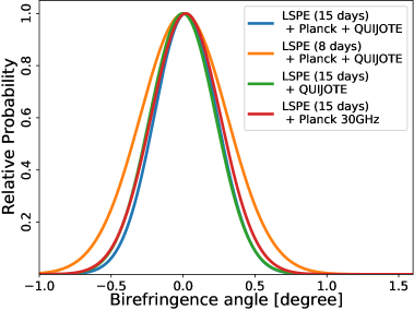
Figure 27: Posterior probability for cosmic birefringence angle obtained with the pixel-based likelihood.

6 Conclusion

The Large Scale Polarization Explorer is a program dedicated to the measurement of the CMB polarization and its B-mode component in particular. We have presented the instruments’ design and a detailed forecast of its performance. LSPE can put an upper limit to the tensor-to-scalar ratio at the level of $r<0.015$ at 95% confidence level, and can detect a signal corresponding to $r=0.03$ with 99.7% confidence. Moreover, LSPE can improve constraints on other parameters, like the optical depth of the Universe to the CMB, $\tau$, and the rotation angle originated by a cosmic birefringence. This analysis is obtained by a full set of end-to-end simulations, including detailed noise estimation, instrument observations (for each detector), contamination by foregrounds, map-making, component separation with realistic foreground residuals, and cosmological parameter extraction with pixel-based likelihood. The assumption about systematic effects is that their contribution can be reduced to below the noise level by means of stringent requirements at design level and by system level calibration. We also present techniques for the control and removal of HWP synchronous systematic effects, including the case of HWP rotational instability.

With its rotating HWP, LSPE-SWIPE represents an important pathfinder of the forthcoming LiteBIRD mission from the point of view of the instrument requirements, instrument design, calibration, control of systematic effects, and data analysis.

Appendix A LSPE-SWIPE scanning and modulation parameters

Parameter	variable	value
Precession period	$T_{\text{Earth}}$	$\sim$24\text{\thinspace}\mathrm{h}\mathrm{r}\mathrm{s}$$
Precession velocity	$\omega_{\text{Earth}}$	$\sim$73\text{\thinspace}\mathrm{\SIUnitSymbolMicro}\mathrm{r}\mathrm{a}\mathrm{d}\thinspace\mathrm{s}^{-1}$$
Precession angle1	$\alpha_{\text{p}}$	$\sim 12-$23\text{\thinspace}\mathrm{\SIUnitSymbolDegree}$$
Payload spin period	$T_{\text{payload}}$	$8.6\text{\thinspace}\mathrm{m}\mathrm{i}\mathrm{n}$
Payload spin rate	$f_{\text{payload}}$	$1.93\text{\thinspace}\mathrm{m}\mathrm{H}\mathrm{z}$
Payload spin velocity	$\omega_{\text{payload}}$	$12.1\text{\thinspace}\mathrm{m}\mathrm{r}\mathrm{a}\mathrm{d}\thinspace\mathrm{s}^{-1}$ $\simeq$$0.7\text{\thinspace}\mathrm{\SIUnitSymbolDegree}\thinspace\mathrm{s}^{-1}$
Zenith angle	$\beta$	$45\text{\thinspace}\mathrm{\SIUnitSymbolDegree}$
Altitude range (combined with FOV)2	$\Delta\beta$	$\pm$10\text{\thinspace}\mathrm{\SIUnitSymbolDegree}$\pm$10\text{\thinspace}\mathrm{\SIUnitSymbolDegree}$$
Max in sky speed3	$\omega_{\text{payload}}\sin\beta_{\text{max}}$	$\sim$0.63\text{\thinspace}\mathrm{\SIUnitSymbolDegree}\thinspace\mathrm{s}^{-1}$$
HWP period	$T_{\text{HWP}}$	$2.0\text{\thinspace}\mathrm{s}$
HWP rate	$f_{\text{HWP}}$	$0.5\text{\thinspace}\mathrm{H}\mathrm{z}$
HWP velocity	$\omega_{\text{HWP}}$	$3.14\text{\thinspace}\mathrm{r}\mathrm{a}\mathrm{d}\thinspace\mathrm{s}^{-1}$
Modulation period	$T_{\text{mod}}=T_{\text{HWP}}/4$	$0.5\text{\thinspace}\mathrm{s}$
Modulation rate	$f_{\text{mod}}=4f_{\text{HWP}}$	$2.0\text{\thinspace}\mathrm{H}\mathrm{z}$
Modulations per FWHM4	$N_{\text{mod}}$	4.5

¹Depending on launch latitude
²The first interval is due to telescope altitude range, the second to the FOV aperture
³Maximum scanning speed of a detector in the sky
⁴Number of modulation periods in a beam FWHM

Table 13: LSPE-SWIPE baseline parameters of observation and modulation strategy. See figure 1, right panel, for reference.

The driving parameter to define the modulator spin rate is the lowest value between detector time constant, cut-off frequency and maximum modulation frequency. The TES developed for LSPE-SWIPE have a typical time constant $\tau_{\text{LP}}=$30\text{\thinspace}\mathrm{m}\mathrm{s}$$. To first approximation, this can be modeled as a single pole low-pass filter, with transfer function

$$H(\omega)=\frac{1}{1+j\omega\tau_{\text{LP}}}=\frac{1}{1+j2\pi f\tau_{\text{LP}}},$$ (A.1)

($\omega$ being the angular frequency here) with cut-off frequency $f_{\tau_{\text{LP}}}=1/(2\pi\tau_{\text{LP}})=$5.3\text{\thinspace}\mathrm{H}\mathrm{z}$$. The HWP can spin up to $f_{\text{HWP}}=$1.5\text{\thinspace}\mathrm{H}\mathrm{z}$$, which corresponds to a modulation frequency $f_{\text{mod}}=4f_{\text{HWP}}=$6\text{\thinspace}\mathrm{H}\mathrm{z}$$. The limiting term is then the detector’s time constant. In order to limit the sensitivity degradation due to the low-pass filtering, considering that most of the polarization signal lies in the $[3,5]f_{\text{HWP}}$ range, we set the HWP spin rate to $f_{\text{HWP}}=$0.5\text{\thinspace}\mathrm{H}\mathrm{z}$$. Most of the polarization signal lies then in the $[1.5,2.5]$ Hz range. The transfer function attenuation at $f_{\text{max}}=$2.5\text{\thinspace}\mathrm{H}\mathrm{z}$$ is

$$|H(f_{\text{max}})|=\frac{1}{\sqrt{1+(2\pi f_{\text{max}}\tau_{\text{LP}})^{2}}}=0.9$$

In order to set the payload angular velocity, we approximate the angular response as a Gaussian profile with standard deviation $\sigma_{b}=\theta_{\text{FWHM}}/(2{\sqrt{2\ln 2}})$; given a scanning speed $\omega_{\text{payload}}$, we convert the angular width into a temporal width $\sigma_{t}=\sigma_{b}/(\omega_{\text{payload}}\sin\beta_{\text{max}})$ where $\sin\beta_{\text{max}}=0.9$ accounts for the altitude projection effect; this can be converted into a frequency width

$$\sigma_{f}=\frac{1}{2\pi\sigma_{t}}=\frac{\omega_{\text{payload}}\sin\beta_{\text{max}}}{2\pi\sigma_{b}};$$

we require that $3\sigma_{f}\leq f_{\text{HWP}}$, so that 99.7% of the signal lies in the $[3,5]\thinspace f_{\text{HWP}}$ range. The condition is then:

$$3\frac{\omega_{\text{payload}}\sin\beta_{\text{max}}}{2\pi\sigma_{b}} \leq f_{\text{HWP}}$$

$$\omega_{\text{payload}} \leq\frac{2\pi\sigma_{b}f_{\text{HWP}}}{3\sin\beta_{\text{max}}}=$0.695\text{\thinspace}\mathrm{\SIUnitSymbolDegree}\thinspace\mathrm{s}^{-1}$$$

$$T_{\text{payload}} \geq 8.6\thinspace\text{min}.$$ (A.2)

As a baseline, we adopt $T_{\text{payload}}=8.6$ min. A beam FWHM is covered $N_{\text{mod}}$ times the HWP modulation period, with

$$N_{\text{mod}}=\frac{\theta_{\text{FWHM}}}{\omega_{\text{payload}}\sin\beta_{\text{max}}}4f_{\text{HWP}}=4.5$$

The complete list of observing parameters for LSPE-SWIPE is reported in table 13.

Appendix B Instrument simulators

Simulators are key elements for instrument design and for data analysis. In the design phase, they allow to predict the scientific performance of the instruments and the impact of systematic effects. In the data analysis phase, they allow to run Monte Carlo realizations of the observations, which are necessary to estimate instrumental biases, to measure transfer functions, and to propagate uncertainties.

The instrument simulator of LSPE-Strip is written in the Julia language [148] and takes advantage of Message Passing Interface (MPI) libraries to parallelize the computation. It is a modular package containing the following components:

• Instrument database containing the configuration of the focal plane and the characteristics of each polarimetric chain to be integrated in the instrument;

• Pointing generation: starting from the configuration and behavior in time of the telescope motors, it produces a timestream of pointing information;

• White noise and $1/f$ noise generation;

• Destriping;

• Map-making.

Being based on a dynamic language like Julia, every module can either be called interactively in a Jupyter notebook or run on a High Performance Computing (HPC) cluster.

The instrument simulator of LSPE-SWIPE consists in a parallel Fortran-90 code which takes as input:

• the number of detectors;

• the detector’s positions in the focal plane;

• the detector’s noise, in terms of NET and $1/f$ knee frequency;

• the mission starting date and duration;

• the angular response in the sky of each detector, as a 2d matrix; this is convolved in pixel space, in a radius specified also as input parameter;

• the HWP operation strategy (stepping, spinning, spinning rate, stepping period);

• the level of HWP synchronous systematic effects, as a signal in $\text{\thinspace}\mathrm{\SIUnitSymbolMicro}\mathrm{K}_{CMB}$ at the HWP spinning frequency and its harmonics;

• HWP angle offset, angular velocity instability, and error in angle measurement;

• timeline filter (high-pass, low-pass, band-pass, notch-filter);

• map-making algorithm details, as simple re-binning, or iterative destriping.

It generates in output:

• timeline of each detector;

• maps of each detector;

• map of combined detectors;

• coverage map;

• noise covariance $3\times 3$ matrix for each observed pixel.

Both simulators can take as input sky maps of any kind. In the analysis presented in this paper, the sky maps have been generated with HEALPix code, for CMB maps, and PySM for foregrounds maps, as detailed in section 5.1. The atmospheric noise is not included in the simulations, but only the atmospheric background power and the corresponding white noise. Noise correlation among different detectors can be included in the SWIPE simulator, but are not included in this analysis. Similarly, realistic beams (angular response) of the telescope can be used, including sidelobes, but only symmetrical main-beams have been considered in this work. In particular for SWIPE, the presence of the HWP strongly attenuates the impact of beam asymmetries. On the other side, beam sidelobes are potentially strong sources of contamination if not properly measured or modeled, and removed from timelines and maps.

Appendix C Atmospheric fluctuations estimation for Strip

The atmospheric fluctuations are very difficult to model and forecast. For this reason, a statistical approach is mandatory. Since we are interested in assessing the atmospheric transparency and its medium-time fluctuations (seasonal and day/night cycles), the atmospheric model has to rely on the statistical fluctuations of the PWV, TS (Surface Temperature), and $P_{0}$ (Surface Pressure). For each hour of each month, we have created the cumulative distribution functions (CDFs) of weather parameters used by the am software to evaluate the atmospheric brightness temperature. To build the CDFs we have used the ERA-5 reanalysis dataset, which estimates the atmosphere’s history using a numerical model to assimilate historical measurements. We then use the simulation-framework Cmb Atmospheric Library (CAL [149]), to estimate the contribution of the seasonal atmospheric fluctuations. In figure 28 we show the statistical water vapor seasonal and daily fluctuations that result from 40 years, hourly time sampled, of ERA-5 reanalysis data. The PWV fluctuations are presented at two different CL: 50% and 95%. The first one is the most representative because it does not contain the samples with bad weather conditions, when the telescope does not observe, while the second one represents the average Tenerife atmosphere behavior.

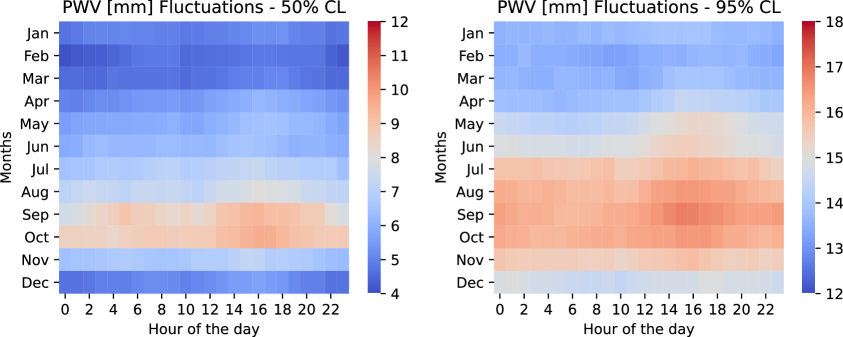
Figure 28: Daily and seasonal fluctuations of the PWV in mm above Pico del Teide - Tenerife. We can appreciate the low daily PWV fluctuations compared to the seasonal ones.

We are working on completing the final results about the fluctuation of the atmospheric temperature. This argument will be the main topic of a dedicated paper that will be released in late 2021.

Appendix D LSPE-SWIPE time response knowledge requirements

The TES detectors of LSPE-SWIPE have an intrinsic time response. Their temporal transfer function $H(\omega)$ can be approximated by a single pole low pass filter, as in equation A.1. More precisely, the time transfer function is characterized by an amplitude, $|H|$ (gain effect) and a phase $\Phi(H)$ (time delay effect). The time delay is

$$\Delta t=\frac{\Phi(H)}{\omega},$$

where $\omega=2\pi f$ is the signal angular frequency of interest, 3 to $5\omega_{\text{HWP}}$ in our case. During this time, the HWP moves of an angle

$$\Delta\theta_{\text{HWP}}=\omega_{\text{HWP}}\Delta t=\Phi(H)\frac{\omega_{\text{HWP}}}{\omega}.$$

This time delay is deconvolved in the analysis pipeline. An error in the knowledge of the transfer function phase has the same effect of an error on the knowledge of the HWP angle. Given the requirement on the HWP angle knowledge, $\Delta\theta_{\text{HWP}}$, we can set the requirement on the knowledge of the transfer function phase as:

$$\Delta\Phi=\frac{\omega}{\omega_{\text{HWP}}}\Delta\theta_{\text{HWP}}=3\Delta\theta_{\text{HWP}}=$42\text{\thinspace}\mathrm{\SIUnitSymbolArcminute}$=12\times 10^{-3}\thinspace\text{rad}$$ (D.1)

where we have considered that the frequencies of interest range from $3f_{\text{HWP}}$. We can express this requirement in terms of the level of knowledge of the time constant $\tau_{\text{LP}}$ of a single pole low-pass filter, considering that $\tan\Phi=-\omega\tau_{\text{LP}}$. An error on the time constant $\Delta{\tau_{\text{LP}}}$ generates an error on the phase

$$\Delta\Phi=\frac{\omega}{(\omega\tau_{\text{LP}})^{2}+1}\Delta{\tau_{\text{LP}}}.$$

Inverting

$$\Delta{\tau_{\text{LP}}}=\frac{(\omega\tau_{\text{LP}})^{2}+1}{\omega}\Delta\Phi=\frac{(\omega\tau_{\text{LP}})^{2}+1}{\omega_{\text{HWP}}}\Delta\theta_{\text{HWP}},$$

where we have used equation D.1. With a time constant $\tau_{\text{LP}}=$30\text{\thinspace}\mathrm{m}\mathrm{s}$$ and a frequency in the 1.5 to $2.5\text{\thinspace}\mathrm{H}\mathrm{z}$ range, this means a requirement:

$$\Delta{\tau_{\text{LP}}}\simeq$1.5\text{\thinspace}\mathrm{m}\mathrm{s}$$$ (D.2)

(relative error $\Delta{\tau_{\text{LP}}}/\tau_{\text{LP}}=5\%$). Also in this case, the requirement will be more stringent if considered jointly with other effects.

Appendix E LSPE-SWIPE iterative map-making

We briefly describe the notch filters and iterative map-making used by the SWIPE instrument simulator pipeline to remove systematic effects appearing at the HWP spin frequency and harmonicsm, and recover the filtered signal.

The notch filters are defined as

$$F(f)=\begin{cases}1&\text{if $f\leq f_{1}$}\\ 0.5\left(1+\cos\left(\pi\frac{f-f_{1}}{f_{2}-f_{1}}\right)\right)&\text{if $f_{1}<f\leq f_{2}$}\\ 0&\text{if $f_{2}<f\leq f_{3}$}\\ 0.5\left(1-\cos\left(\pi\frac{f-f_{3}}{f_{4}-f_{3}}\right)\right)&\text{if $f_{3}<f\leq f_{4}$}\\ 1&\text{if $f>f_{4}$}\\ \end{cases}$$ (E.1)

where $f_{1}=f_{0}-2\Delta f$, $f_{2}=f_{0}-\Delta f$, $f_{3}=f_{0}+\Delta f$, and $f_{4}=f_{0}+2\Delta f$ are the frequencies where the filter starts to drop, reaches 0, starts to rise, reaches 1 respectively; $f_{0}$ is the notch filter frequency, and $\Delta f$ is the notch filter width. In simulations, we set $f_{0}$ to the HWP spin frequency and harmonics, and $\Delta f=$1\text{\thinspace}\mathrm{m}\mathrm{H}\mathrm{z}$$, lower than the payload default spin rate, set at $1.93\text{\thinspace}\mathrm{m}\mathrm{H}\mathrm{z}$ (table 13). The notch filter applied at 4 times the HWP spin rate, $4f_{\text{HWP}}$, can remove part of the signal at the largest scales in the sky. This happens despite the fact that the payload spin rate is above the notch filter width. In fact, the sky signal is not exactly periodic, and part of it is spread in the interval $[4f_{\text{HWP}}\pm f_{\text{payload}}]$ , i.e. within the spin rate frequency from modulation frequency. This signal is recovered by an iterative mapmaking process.

In the following, $P$ is the pointing matrix, $M_{P}$ is the rebinning matrix; $\otimes$ means a filtering. The iterative procedure is applied to the timeline $d_{j}$ of the $j$-th detector:

• each timeline is notch-filtered to remove the contamination $\tilde{d}_{j}=F\otimes d_{j}$;

• all filtered timelines are combined in a first map, by simple rebin $m_{0}=\sum_{j}M_{P}\tilde{d}_{j}$;

• here starts the iteration, from $i=0$;

• a synthetic timeline is produced for each detector: $h_{j}=Pm_{i}$;

• the synthetic timeline is filtered by $1-F$, to recover the missing signal: $\tilde{h}_{j,i}=(1-F)\otimes h_{j,i}$;

• the filtered synthetic timeline is added to the filtered original timeline: $d_{j,i}=\tilde{d}_{j}+\tilde{h}_{j,i}$;

• a new map is produced: $m_{i+1}=\sum_{j}M_{P}\tilde{d}_{j,i}$, and the procedure is iterated.

Testing different numbers of iterations, we have found that 50 iterations represents a good trade-off between computational time and residual signal in the map with filtered timelines.

References

- [1] U. Seljak and M. Zaldarriaga, Signature of gravity waves in the polarization of the microwave background, Phys. Rev. Lett. 78 (1997) 2054.
- [2] M. Kamionkowski and E.D. Kovetz, The Quest for B Modes from Inflationary Gravitational Waves, Annu. Rev. Astron. Astr. 54 (2016) 227.
- [3] Planck Collaboration, N. Aghanim, Y. Akrami, F. Arroja, M. Ashdown, J. Aumont et al., Planck 2018 results. I. Overview and the cosmological legacy of Planck, A&A 641 (2020) A1 [1807.06205].
- [4] M. Tristram, A.J. Banday, K.M. Górski, R. Keskitalo, C.R. Lawrence, K.J. Andersen et al., Planck constraints on the tensor-to-scalar ratio, A&A 647 (2021) A128 [2010.01139].
- [5] P.A.R. Ade, Z. Ahmed, R.W. Aikin, K.D. Alexander, D. Barkats, S.J. Benton et al., Constraints on Primordial Gravitational Waves Using Planck, WMAP, and New BICEP2/Keck Observations through the 2015 Season, Phys. Rev. Lett. 121 (2018) 221301 [1810.05216].
- [6] M. Archidiacono, A. Cooray, A. Melchiorri and S. Pandolfi, Cmb neutrino mass bounds and reionization, Phys. Rev. D 82 (2010) 087302.
- [7] R. Allison, P. Caucal, E. Calabrese, J. Dunkley and T. Louis, Towards a cosmological neutrino mass detection, Phys. Rev. D 92 (2015) 123535.
- [8] J.A. Grayson, P.A.R. Ade, Z. Ahmed, K.D. Alexander, M. Amiri, D. Barkats et al., BICEP3 performance overview and planned Keck Array upgrade, in Millimeter, Submillimeter, and Far-Infrared Detectors and Instrumentation for Astronomy VIII, W.S. Holland and J. Zmuidzinas, eds., vol. 9914 of Society of Photo-Optical Instrumentation Engineers (SPIE) Conference Series, p. 99140S, July, 2016, DOI [1607.04668].
- [9] L. Moncelsi, P.A.R. Ade, A. Z, M. Amiri, D. Barkats, R.B. Thakur et al., Receiver development for BICEP Array, a next-generation CMB polarimeter at the South Pole, in Millimeter, Submillimeter, and Far-Infrared Detectors and Instrumentation for Astronomy X, J. Zmuidzinas and J.-R. Gao, eds., vol. 11453, pp. 189 – 206, International Society for Optics and Photonics, SPIE, 2020, DOI.
- [10] K. Harrington, T. Marriage, A. Ali, J.W. Appel, C.L. Bennett, F. Boone et al., The Cosmology Large Angular Scale Surveyor, in Millimeter, Submillimeter, and Far-Infrared Detectors and Instrumentation for Astronomy VIII, W.S. Holland and J. Zmuidzinas, eds., vol. 9914 of Society of Photo-Optical Instrumentation Engineers (SPIE) Conference Series, p. 99141K, July, 2016, DOI [1608.08234].
- [11] A. Suzuki, P. Ade, Y. Akiba, C. Aleman, K. Arnold, C. Baccigalupi et al., The Polarbear-2 and the Simons Array Experiments, J. Low Temp. Phys. 184 (2016) 805 [1512.07299].
- [12] J.T. Sayre, C.L. Reichardt, J.W. Henning, P.A.R. Ade, A.J. Anderson, J.E. Austermann et al., Measurements of B -mode polarization of the cosmic microwave background from 500 square degrees of SPTpol data, Phys. Rev. D 101 (2020) 122003 [1910.05748].
- [13] B.A. Benson, P.A.R. Ade, Z. Ahmed, S.W. Allen, K. Arnold, J.E. Austermann et al., SPT-3G: a next-generation cosmic microwave background polarization experiment on the South Pole telescope, in Millimeter, Submillimeter, and Far-Infrared Detectors and Instrumentation for Astronomy VII, W.S. Holland and J. Zmuidzinas, eds., vol. 9153, pp. 552 – 572, International Society for Optics and Photonics, SPIE, 2014, DOI.
- [14] S. Aiola, E. Calabrese, L. Maurin, S. Naess, B.L. Schmitt, M.H. Abitbol et al., The Atacama Cosmology Telescope: DR4 maps and cosmological parameters, J. Cosmol. Astropart. P. 2020 (2020) 047 [2007.07288].
- [15] S.K. Choi, M. Hasselfield, S.-P.P. Ho, B. Koopman, M. Lungu, M.H. Abitbol et al., The Atacama Cosmology Telescope: a measurement of the Cosmic Microwave Background power spectra at 98 and 150 GHz, J. Cosmol. Astropart. P. 2020 (2020) 045 [2007.07289].
- [16] P. Ade, J. Aguirre, Z. Ahmed, S. Aiola, A. Ali, D. Alonso et al., The Simons Observatory: science goals and forecasts, J. Cosmol. Astropart. P. 2019 (2019) 056 [1808.07445].
- [17] S. Oguri, J. Choi, T. Damayanthi, M. Hattori, M. Hazumi, H. Ishitsuka et al., GroundBIRD: Observing Cosmic Microwave Polarization at Large Angular Scale with Kinetic Inductance Detectors and High-Speed Rotating Telescope, J. Low Temp. Phys. 184 (2016) 786.
- [18] J.C. Hamilton, L. Mousset, E.S. Battistelli, M.A. Bigot-Sazy, P. Chanial, R. Charlassier et al., QUBIC I: Overview and ScienceProgram, arXiv e-prints (2020) arXiv:2011.02213 [2011.02213].
- [19] The CMB-S4 Collaboration, :, K. Abazajian, G.E. Addison, P. Adshead, Z. Ahmed et al., CMB-S4: Forecasting Constraints on Primordial Gravitational Waves, arXiv e-prints (2020) arXiv:2008.12619 [2008.12619].
- [20] R. Gualtieri, J.P. Filippini, P.A.R. Ade, M. Amiri, S.J. Benton, A.S. Bergman et al., SPIDER: CMB Polarimetry from the Edge of Space, J. Low Temp. Phys. 193 (2018) 1112 [1711.10596].
- [21] N.N. Gandilo, P.A.R. Ade, D. Benford, C.L. Bennett, D.T. Chuss, J.L. Dotson et al., The Primordial Inflation Polarization Explorer (PIPER), in Millimeter, Submillimeter, and Far-Infrared Detectors and Instrumentation for Astronomy VIII, W.S. Holland and J. Zmuidzinas, eds., vol. 9914 of Society of Photo-Optical Instrumentation Engineers (SPIE) Conference Series, p. 99141J, July, 2016, DOI [1607.06172].
- [22] S. Hanany, M. Alvarez, E. Artis, P. Ashton, J. Aumont, R. Aurlien et al., PICO: Probe of Inflation and Cosmic Origins, in Bulletin of the American Astronomical Society, vol. 51, p. 194, Sept., 2019 [1908.07495].
- [23] M. Hazumi, P.A.R. Ade, Y. Akiba, D. Alonso, K. Arnold, J. Aumont et al., LiteBIRD: A Satellite for the Studies of B-Mode Polarization and Inflation from Cosmic Background Radiation Detection, J. Low Temp. Phys. 194 (2019) 443.
- [24] H. Sugai, P.A.R. Ade, Y. Akiba, D. Alonso, K. Arnold, J. Aumont et al., Updated Design of the CMB Polarization Experiment Satellite LiteBIRD, J. Low Temp. Phys. (2020) [2001.01724].
- [25] P. de Bernardis, S. Aiola, G. Amico, E. Battistelli, A. Coppolecchia, A. Cruciani et al., SWIPE: a bolometric polarimeter for the Large-Scale Polarization Explorer, in Millimeter, Submillimeter, and Far-Infrared Detectors and Instrumentation for Astronomy VI, vol. 8452 of Proc. SPIE, p. 84523F, Sept., 2012, DOI [1208.0282].
- [26] S. Aiola, G. Amico, P. Battaglia, E. Battistelli, A. Baó, P. de Bernardis et al., The Large-Scale Polarization Explorer (LSPE), in Ground-based and Airborne Instrumentation for Astronomy IV, vol. 8446 of Proc. SPIE, p. 84467A, Sept., 2012, DOI.
- [27] M. Bersanelli, A. Mennella, G. Morgante, M. Zannoni, G. Addamo, A. Baschirotto et al., A coherent polarimeter array for the Large Scale Polarization Explorer (LSPE) balloon experiment, in Ground-based and Airborne Instrumentation for Astronomy IV, vol. 8446 of Proc. SPIE, p. 84467C, Sept., 2012, DOI [1208.0164].
- [28] L. Lamagna, G. Addamo, P.A.R. Ade, C. Baccigalupi, A.M. Baldini, P.M. Battaglia et al., Progress report on the Large Scale Polarization Explorer, J. Low Temp. Phys. (2020) arXiv:2005.01187 [2005.01187].
- [29] F. Incardona, Observing the polarized Cosmic Microwave Background from the Earth : scanning strategy and polarimeters test for the LSPE / STRIP instrument, Ph.D. thesis, University of Milan, 2020.
- [30] F. Incardona, M. Benetti, M. Bersanelli, C. Franceschet, D. Maino, A. Mennella et al., Preliminary scanning strategy analysis for the LSPE-STRIP instrument, in Society of Photo-Optical Instrumentation Engineers (SPIE) Conference Series, vol. 10708, p. 107082F, Jul, 2018, DOI.
- [31] N. Krachmalnicoff, E. Carretti, C. Baccigalupi, G. Bernardi, S. Brown, B.M. Gaensler et al., S-PASS view of polarized Galactic synchrotron at 2.3 GHz as a contaminant to CMB observations, Astron. Astrophys. 618 (2018) A166 [1802.01145].
- [32] J.A. Castro-Almazán, C. Muñoz-Tuñón, B. García-Lorenzo, G. Pérez-Jordán, A.M. Varela and I. Romero, Precipitable Water Vapour at the Canarian Observatories (Teide and Roque de los Muchachos) from routine GPS, in Observatory Operations: Strategies, Processes, and Systems VI, vol. 9910 of Society of Photo-Optical Instrumentation Engineers (SPIE) Conference Series, p. 99100P, Jul, 2016, DOI.
- [33] C.M. Gutiérrez, R. Rebolo, R.A. Watson, R.D. Davies, A.W. Jones and A.N. Lasenby, The Tenerife Cosmic Microwave Background Maps: Observations and First Analysis, Astrophys. J. 529 (2000) 47 [astro-ph/9903196].
- [34] B. Femenía, R. Rebolo, C.M. Gutiérrez, M. Limon and L. Piccirillo, The Instituto de Astrofísica de Canarias-Bartol Cosmic Microwave Background Anisotropy Experiment: Results of the 1994 Campaign, Astrophys. J. 498 (1998) 117 [astro-ph/9711225].
- [35] D.L. Harrison, J.A. Rubiño-Martin, S.J. Melhuish, R.A. Watson, R.D. Davies, R. Rebolo et al., A measurement at the first acoustic peak of the cosmic microwave background with the 33-GHz interferometer, Mon. Not. Roy. Astron. Soc. 316 (2000) L24 [astro-ph/0004357].
- [36] S. Fernández-Cerezo, C.M. Gutiérrez, R. Rebolo, R.A. Watson, R.J. Hoyland, S.R. Hildebrandt et al., Observations of the cosmic microwave background and galactic foregrounds at 12-17GHz with the COSMOSOMAS experiment, Mon. Not. Roy. Astron. Soc. 370 (2006) 15 [astro-ph/0601203].
- [37] R.A. Watson, P. Carreira, K. Cleary, R.D. Davies, R.J. Davis, C. Dickinson et al., First results from the Very Small Array - I. Observational methods, Mon. Not. Roy. Astron. Soc. 341 (2003) 1057 [astro-ph/0205378].
- [38] J.A. Rubiño-Martín, R. Rebolo, M. Aguiar, R. Génova-Santos, F. Gómez-Reñasco, J.M. Herreros et al., The QUIJOTE-CMB experiment: studying the polarisation of the galactic and cosmological microwave emissions, in Ground-based and Airborne Telescopes IV, vol. 8444 of Society of Photo-Optical Instrumentation Engineers (SPIE) Conference Series, p. 84442Y, Sep, 2012, DOI.
- [39] K. Lee, J. Choi, R.T. Génova-Santos, M. Hattori, M. Hazumi, S. Honda et al., GroundBIRD: A CMB Polarization Experiment with MKID Arrays, Journal of Low Temperature Physics 200 (2020) 384 [2011.07705].
- [40] A.C. Taylor, Clover - A B-mode polarization experiment, New Astron. Rev. 50 (2006) 993 .
- [41] C. Franceschet, S. Realini, A. Mennella, G. Addamo, A. Baú, P.M. Battaglia et al., The STRIP instrument of the Large Scale Polarization Explorer: microwave eyes to map the Galactic polarized foregrounds, in Millimeter, Submillimeter, and Far-Infrared Detectors and Instrumentation for Astronomy IX, vol. 10708 of Society of Photo-Optical Instrumentation Engineers (SPIE) Conference Series, p. 107081G, Jul, 2018, DOI.
- [42] S. Realini, C. Franceschet and A. Mennella, Modelling the radiation pattern of a dual circular polarization system, J. Instrum. 14 (2019) P03005.
- [43] O.A. Peverini, G. Virone, F. Del Torto, C. Franceschet, F. Villa, M. Lumia et al., Q-band antenna-feed system for the Large Scale Polarization Explorer balloon experiment, in 2015 International Conference on Electromagnetics in Advanced Applications (ICEAA), pp. 883–886, IEEE, sep, 2015, DOI.
- [44] F. Del Torto, M. Bersanelli, F. Cavaliere, A. De Rosa, O. D’Arcangelo, C. Franceschet et al., W-band prototype of platelet feed-horn array for CMB polarisation measurements, J. Instrum. 6 (2011) 6009 [1107.1157].
- [45] S.Y. Eom and Y.B. Korchemkin, A New Comb Circular Polarizer Suitable for Millimeter-Band Application, ETRI Journal 28 (2006) 656.
- [46] G. Virone, O.A. Peverini, M. Lumia, G. Addamo and R. Tascone, Platelet Orthomode Transducer for Q-Band Correlation Polarimeter Clusters, IEEE T. Microw. Theory 62 (2014) 1487.
- [47] QUIET Collaboration, D. Araujo, C. Bischoff, A. Brizius, I. Buder, Y. Chinone et al., Second season QUIET observations: Measurements of the cosmic microwave background polarization power spectrum at 95 GHz, Astrophys. J. 760 (2012) [1207.5034].
- [48] Y.-L. Chen, T. Chiueh and H.-F. Teng, A 77-118 GHz RESONANCE-FREE SEPTUM POLARIZER, Astrophys. J., Suppl. Ser. 211 (2014) 11.
- [49] QUIET Collaboration, C. Bischoff, A. Brizius, I. Buder, Y. Chinone, K. Cleary et al., First Season QUIET Observations: Measurements of Cosmic Microwave Background Polarization Power Spectra at 43 GHz in the Multipole Range , Astrophys. J. 741 (2011) 111 [1012.3191].
- [50] A. Iarocci, P. Benedetti, F. Caprara, A. Cardillo, F. di Felice, G. di Stefano et al., PEGASO: An ultra light long duration stratospheric payload for polar regions flights, Adv. Space Res. 42 (2008) 1633.
- [51] S. Peterzen, S. Masi, P. Dragoy, R. Ibba and D. Spoto, Long Duration Balloon flights development. (Italian Space Agency), Mem. Soc. Astron. Italiana 79 (2008) 792.
- [52] Masi, Silvia, Coppolecchia, A., Battistelli, E., de Bernardis, P., Columbro, F., D´Alessandro, G. et al., Balloon-borne cosmic microwave background experiments, EPJ Web Conf. 209 (2019) 01046.
- [53] P. de Bernardis, S. Masi and OLIMPO and LSPE Teams, Precision CMB measurements with long-duration stratospheric balloons: activities in the Arctic, in Astrophysics from Antarctica, M.G. Burton, X. Cui and N.F.H. Tothill, eds., vol. 288 of IAU Symposium, pp. 208–213, Jan., 2013, DOI.
- [54] F. Piacentini, A. Coppolecchia, P. de Bernardis, G. Di Stefano, A. Iarocci, L. Lamagna et al., Winter long duration stratospheric balloons from Polar regions, arXiv e-prints (2018) arXiv:1810.05565 [1810.05565].
- [55] P. de Bernardis, E. Aquilini, A. Boscaleri, M. de Petris, M. Gervasi, L. Martinis et al., ARGO: a balloon-borne telescope for measurements of the millimeter diffuse sky emission, Astron. Astrophys. 271 (1993) 683.
- [56] B.P. Crill, P.A.R. Ade, D.R. Artusa, R.S. Bhatia, J.J. Bock, A. Boscaleri et al., BOOMERANG: A Balloon-borne Millimeter-Wave Telescope and Total Power Receiver for Mapping Anisotropy in the Cosmic Microwave Background, Astrophys. J., Suppl. Ser. 148 (2003) 527 [astro-ph/0206254].
- [57] S. Masi, P.A.R. Ade, J.J. Bock, J.R. Bond, J. Borrill, A. Boscaleri et al., Instrument, method, brightness, and polarization maps from the 2003 flight of BOOMERanG, Astron. Astrophys. 458 (2006) 687 [astro-ph/0507509].
- [58] A. Benoît, P. Ade, A. Amblard, R. Ansari, E. Aubourg, J. Bartlett et al., Archeops: a high resolution, large sky coverage balloon experiment for mapping cosmic microwave background anisotropies, Astropart. Phys. 17 (2002) 101 [astro-ph/0106152].
- [59] S. Masi, M. Calvo, L. Conversi, P. de Bernardis, M. de Petris, G. de Troia et al., A balloon-borne survey of the mm/sub-mm sky: OLIMPO, in 17th ESA Symposium on European Rocket and Balloon Programmes and Related Research, B. Warmbein, ed., vol. 590 of ESA Special Publication, pp. 581–586, Aug., 2005.
- [60] A. Paiella, A. Coppolecchia, L. Lamagna, P. Ade, E. Battistelli, M.G. Castellano et al., Kinetic inductance detectors for the OLIMPO experiment: design and pre-flight characterization, J. Cosmol. Astropart. P. 2019 (2019) 039.
- [61] S. Masi, P. de Bernardis, A. Paiella, F. Piacentini, L. Lamagna, A. Coppolecchia et al., Kinetic Inductance Detectors for the OLIMPO experiment: in-flight operation and performance, J. Cosmol. Astropart. P. 2019 (2019) 003 [1902.08993].
- [62] A. Boscaleri, V. Venturi and R. Colzi, Time-domain computer simulation program as first step of a full digital high-precision pointing system for platform in balloon-borne remote sensing, in Infrared Technology XVI, I.J. Spiro, ed., vol. 1341, pp. 58 – 65, International Society for Optics and Photonics, SPIE, 1990, DOI.
- [63] A. Boscaleri, A time domain design technique for high precision full digital pointing system in balloon-borne remote infrared sensing, in Acquisition, Tracking, and Pointing IV, S. Gowrinathan, ed., vol. 1304, International Society for Optics and Photonics, SPIE, 1990, DOI.
- [64] A. Boscaleri, V. Venturi and D. Tirelli, The ARGO experiment pointing system as an example for other single-axis platform pointing systems, Meas. Sci. Technol. 5 (1994) 190.
- [65] F. Nati, P. de Bernardis, A. Iacoangeli, S. Masi, A. Benoit and D. Yvon, A fast star sensor for balloon payloads, Rev. Sci. Instrum. 74 (2003) 4169.
- [66] J.F. Macías-Pérez, G. Lagache, B. Maffei, K. Ganga, A. Bourrachot, P. Ade et al., Archeops in-flight performance, data processing, and map making, Astron. Astrophys. 467 (2007) 1313 [astro-ph/0603665].
- [67] P. Palumbo, E. Aquilini, P. Cardoni, P. de Bernardis, A. De Ninno, L. Martinis et al., Balloon-borne 3He cryostat for millimetre bolometric photometry, Cryogenics 34 (1994) 1001.
- [68] S. Masi, P. Cardoni, P. de Bernardis, F. Piacentini, A. Raccanelli and F. Scaramuzzi, A long duration cryostat suitable for balloon borne photometry, Cryogenics 39 (1999) 217.
- [69] J.P. Bernard, P. Ade, Y. André, J. Aumont, L. Bautista, N. Bray et al., PILOT: a balloon-borne experiment to measure the polarized FIR emission of dust grains in the interstellar medium, Exp. Astron. 42 (2016) 199.
- [70] A. Coppolecchia, L. Lamagna, S. Masi, P. Ade, G. Amico, E. Battistelli et al., The long duration cryogenic system of the olimpo balloon-borne experiment: design and in-flight performance, Cryogenics (2020) 103129.
- [71] G. Coppi, P. de Bernardis, A.J. May, S. Masi, M. McCulloch, S.J. Melhuish et al., Developing a long duration 3He fridge for the LSPE-SWIPE instrument, in Proc. SPIE, vol. 9912 of Society of Photo-Optical Instrumentation Engineers (SPIE) Conference Series, p. 991265, SPIE (2016), DOI.
- [72] K. Zilic, A. Aboobaker, F. Aubin, C. Geach, S. Hanany, N. Jarosik et al., A double vacuum window mechanism for space-borne applications, Rev. Sci. Instrum. 88 (2017) .
- [73] G. dall’Oglio, P. de Bernardis, S. Masi and F. Melchiorri, Measurement of the 3K Cosmic Background Noise in the Far Infrared, in Early Evolution of the Universe and its Present Structure, G.O. Abell and G. Chincarini, eds., vol. 104 of IAU Symposium, p. 135, Jan., 1983.
- [74] J.F. Macías-Pérez, G. Lagache, B. Maffei, K. Ganga, A. Bourrachot, P. Ade et al., Archeops in-flight performance, data processing, and map making, Astron. Astrophys. 467 (2007) 1313 [astro-ph/0603665].
- [75] G. D’Alessandro, A. Paiella, A. Coppolecchia, M.G. Castellano, I. Colantoni, P. de Bernardis et al., Ultra high molecular weight polyethylene: Optical features at millimeter wavelengths, Infrared Phys. Technol. 90 (2018) 59 [1803.05228].
- [76] S. Legg, L. Lamagna, G. Coppi, P. de Bernardis, G. Giuliani, R. Gualtieri et al., Development of the multi-mode horn-lens configuration for the LSPE-SWIPE B-mode experiment, in Millimeter, Submillimeter, and Far-Infrared Detectors and Instrumentation for Astronomy VIII, vol. 9914 of Proceeding SPIE, p. 991414, July, 2016, DOI.
- [77] F. Columbro, P.G. Madonia, L. Lamagna, E.S. Battistelli, A. Coppolecchia, P. de Bernardis et al., Swipe multi-mode pixel assembly design and beam pattern measurements at cryogenic temperature, J. Low Temp. Phys. 199 (2020) 312.
- [78] A.C. Ludwig, The definition of cross polarization., IEEE T. Antenn. Propag. 21 (1973) 116.
- [79] G. Pisano, C. Tucker, P.A.R. Ade, P. Moseley and M.W. Ng, Metal mesh based metamaterials for millimetre wave and thz astronomy applications, in 2015 8th UK, Europe, China Millimeter Waves and THz Technology Workshop (UCMMT), pp. 1–4, 2015, DOI.
- [80] G. Pisano, M. Ng, V. Haynes and B. Maffei, A broadband metal-mesh half-wave plate for millimetre wave linear polarisation rotation, in Progress In Electromagnetics Research M, vol. 25, pp. 101–114, 2012, DOI.
- [81] G. Pisano, P. Ade, C. Tucker and M.W. Ng, Large bandwidth mesh half-wave plates for millimetre and thz wave astronomy, in 2015 40th International Conference on Infrared, Millimeter, and Terahertz waves (IRMMW-THz), pp. 1–1, 2015.
- [82] T. Matsumura, H. Kataza, S. Utsunomiya, R. Yamamoto, M. Hazumi and N. Katayama, Design and performance of a prototype polarization modulator rotational system for use in space using a superconducting magnetic bearing, IEEE Trans. Appl. Supercond. 26 (2016) 1.
- [83] B. Johnson, F. Columbro, D. Araujo, M. Limon, B. Smiley, G. Jones et al., A large-diameter hollow-shaft cryogenic motor based on a superconducting magnetic bearing for millimeter-wave polarimetry, Rev. Sci. Instrum. 88 (2017) .
- [84] F. Columbro, P. de Bernardis, L. Lamagna, S. Masi, A. Paiella, F. Piacentini et al., A polarization modulator unit for the mid- and high-frequency telescopes of the LiteBIRD mission, vol. 11443 of Society of Photo-Optical Instrumentation Engineers (SPIE) Conference Series, p. 114436Z, Dec., 2020, DOI.
- [85] F. Columbro, P. de Bernardis and S. Masi, A clamp and release system for superconductive magnetic bearings, Rev. Sci. Instrum. 89 (2018) .
- [86] P. de Bernardis, F. Columbro, S. Masi, A. Paiella and G. Romeo, A simple method to measure the temperature and levitation height of devices rotating at cryogenic temperatures, Rev. Sci. Instrum. 91 (2020) 045118 [https://doi.org/10.1063/5.0005498].
- [87] D. Vaccaro, B. Siri, A.M. Baldini, M. Biasotti, F. Cei, V. Ceriale et al., Tuning the of Titanium Thin Films for Transition-Edge Sensors by Annealing in Argon, J. Low Temp. Phys. 193 (2018) 1122.
- [88] D. Vaccaro, A.M. Baldini, F. Cei, L. Galli, M. Grassi, D. Nicolò et al., "The FDM readout for the LSPE/SWIPE TES bolometers", in Millimeter, Submillimeter, and Far-Infrared Detectors and Instrumentation for Astronomy IX, J. Zmuidzinas and J.-R. Gao, eds., vol. 10708, pp. 732 – 742, International Society for Optics and Photonics, Proc. SPIE, 2018, DOI.
- [89] D. Vaccaro, A. Baldini, F. Cei, L. Galli, M. Grassi, D. Nicolò et al., A frequency domain multiplexing system to readout the TES bolometers on the LSPE/SWIPE experiment, Nucl. Instrum. Meth. A 936 (2019) 169.
- [90] F. Fontanelli, M. Biasotti, A. Bevilacqua and F. Siccardi, The front-end electronics of the LSPE-SWIPE experiment, in Space Telescopes and Instrumentation 2016: Optical, Infrared, and Millimeter Wave, H.A. MacEwen, G.G. Fazio, M. Lystrup, N. Batalha, N. Siegler and E.C. Tong, eds., vol. 9904, pp. 1633 – 1638, International Society for Optics and Photonics, Proc. SPIE, 2016, DOI.
- [91] C. Bischoff, A. Brizius, I. Buder, Y. Chinone, K. Cleary, R.N. Dumoulin et al., THE Q/U IMAGING EXPERIMENT INSTRUMENT, Astrophys. J. 768 (2013) 9.
- [92] K. Cleary, Coherent polarimeter modules for the QUIET experiment, in Society of Photo-Optical Instrumentation Engineers (SPIE) Conference Series, vol. 7741 of Society of Photo-Optical Instrumentation Engineers (SPIE) Conference Series, jul, 2010, DOI.
- [93] S. Paine, The am atmospheric model, Sept., 2019. 10.5281/zenodo.3406496.
- [94] M.N. Afsar, K.A. Korolev, L. Subramanian and I.I. Tkachov, Complex Dielectric Measurements of Materials at Q- Band, V- Band and W- Band Frequencies with High Power Sources, in 2005 IEEE Instrumentationand Measurement Technology Conference Proceedings, vol. 1, pp. 82–87, 2005.
- [95] J.W. Lamb, Miscellaneous data on materials for millimetre and submillimetre optics, J. Infrared. Millim. W. 17 (1996) 1997.
- [96] J.M. Lamarre, Photon noise in photometric instruments at far-infrared and submillimeter wavelengths, Appl. Opt. 25 (1986) 870.
- [97] R. Gualtieri, E.S. Battistelli, A. Cruciani, P. de Bernardis, M. Biasotti, D. Corsini et al., Multi-mode TES Bolometer Optimization for the LSPE-SWIPE Instrument, J. Low Temp. Phys. 184 (2016) 527 [1602.07744].
- [98] M. Dobbs et al., Frequency Multiplexed SQUID Readout of Large Bolometer Arrays for Cosmic Microwave Background Measurements, Rev. Sci. Instrum. 83 (2012) 073113 [1112.4215].
- [99] A. Tartari, A.M. Baldini, F. Cei, L. Galli, M. Grassi, D. Nicolò et al., Development and testing of the fdm read-out of the tes arrays aboard the lspe/swipe balloon-borne experiment, J. Low Temp. Phys. 199 (2020) 212.
- [100] Planck Collaboration III, Planck 2013 results. III. LFI systematic uncertainties, Astron. Astrophys. 571 (2014) A3 [1303.5064].
- [101] Planck Collaboration, P.A.R. Ade, J. Aumont, C. Baccigalupi, A.J. Banday, R.B. Barreiro et al., Planck 2015 results. III. LFI systematic uncertainties, Astron. Astrophys. 594 (2016) A3.
- [102] S. Church, Predicting residual levels of atmospheric sky noise in ground-based observations of the cosmic background radiation, Mon. Not. Roy. Astron. Soc. 272 (1995) 551.
- [103] Planck Collaboration, P.A.R. Ade, N. Aghanim, M. Ashdown, J. Aumont, C. Baccigalupi et al., Planck 2015 results. IV. Low Frequency Instrument beams and window functions, Astron. Astrophys. 594 (2016) A4.
- [104] Planck Collaboration III, Planck 2015 results. III. LFI systematic uncertainties, Astron. Astrophys. 594 (2016) A3 [1507.08853].
- [105] N. Krachmalnicoff, Challenges for Present and Future Cosmic Microwave Background Observations: Systematic Effects and Foreground Emission in Polarization, Ph.D. thesis, University of Milan, 2015.
- [106] G. Montresor, A responsivity calibration strategy for the LSPE-STRIP balloon experiment, Master’s thesis, University of Milan, 2012.
- [107] F. Paonessa, G. Virone, L. Ciorba, G. Addamo, M. Lumia, G. Dassano et al., Design and verification of a Q-Band test source for UAV-based radiation pattern measurements, IEEE Trans. Instrum. Meas. 69 (2020) 9366.
- [108] M. Salatino, P. de Bernardis and S. Masi, Modeling transmission and reflection mueller matrices of dielectric half-wave plates, Journal of Infrared, Millimeter, and Terahertz Waves 38 (2017) 215.
- [109] G. Pisano, G. Savini, P.A.R. Ade, V. Haynes and W.K. Gear, Achromatic half-wave plate for submillimeter instruments in cosmic microwave background astronomy: experimental characterization, Appl. Opt. 45 (2006) 6982.
- [110] Y.D. Takahashi, P.A.R. Ade, D. Barkats, J.O. Battle, E.M. Bierman, J.J. Bock et al., Characterization of the BICEP Telescope for High-precision Cosmic Microwave Background Polarimetry, Astrophys. J 711 (2010) 1141 [0906.4069].
- [111] H. Imada, T. Matsumura, R. Takaku, G. Patanchon, H. Ishino, Y. Sakurai et al., Instrumentally induced spurious polarization of a multi-layer half wave plate for a cmb polarization observation, pp. 61–67, Jan., 2018.
- [112] A. Kusaka, J. Appel, T. Essinger-Hileman, J.A. Beall, L.E. Campusano, H.-M. Cho et al., Results from the Atacama B-mode Search (ABS) experiment, J. Cosmol. Astropart. P. 2018 (2018) 005 [1801.01218].
- [113] T. Essinger-Hileman, A. Kusaka, J.W. Appel, S.K. Choi, K. Crowley, S.P. Ho et al., Systematic effects from an ambient-temperature, continuously rotating half-wave plate, Rev. Sci. Instrum. 87 (2016) 094503 [1601.05901].
- [114] S.A. Bryan, T.E. Montroy and J.E. Ruhl, Modeling dielectric half-wave plates for cosmic microwave background polarimetry using a Mueller matrix formalism, Appl. Opt. 49 (2010) 6313 [1006.3359].
- [115] L. Pagano, P. de Bernardis, G. de Troia, G. Gubitosi, S. Masi, A. Melchiorri et al., CMB polarization systematics, cosmological birefringence, and the gravitational waves background, Phys. Rev. D 80 (2009) 043522 [0905.1651].
- [116] F. Columbro, E.S. Battistelli, A. Coppolecchia, G. D’Alessandro, P. de Bernardis, L. Lamagna et al., The short wavelength instrument for the polarization explorer balloon-borne experiment: Polarization modulation issues, Astron. Nachr. 340 (2019) 83 [1904.01891].
- [117] J. Aumont, J.F. Macías-Pérez, A. Ritacco, N. Ponthieu and A. Mangilli, Absolute calibration of the polarisation angle for future CMB B-mode experiments from current and future measurements of the Crab nebula, Astron. Astrophys. 634 (2020) A100 [1911.03164].
- [118] M. Tucci, E. Martínez-González, P. Vielva and J. Delabrouille, Limits on the detectability of the CMB B-mode polarization imposed by foregrounds, Mon. Not. Roy. Astron. Soc. 360 (2005) 935 [https://academic.oup.com/mnras/article-pdf/360/3/935/3206389/360-3-935.pdf].
- [119] A. Buzzelli, M. Migliaccio, G. de Gasperis, P. de Bernardis, S. Masi and N. Vittorio, Impact of polarized foregrounds on LSPE-SWIPE observations, in J. Phys. Conf. Ser., vol. 956, p. 012002, Jan., 2018, DOI.
- [120] Planck Collaboration, Y. Akrami, M. Ashdown, J. Aumont, C. Baccigalupi, M. Ballardini et al., Planck 2018 results. IV. Diffuse component separation, Astron. Astrophys. 641 (2020) A4 [1807.06208].
- [121] P. Campeti, D. Poletti and C. Baccigalupi, Principal component analysis of the primordial tensor power spectrum, J. Cosmol. Astropart. P. 1909 (2019) 055 [1905.08200].
- [122] R. Stompor, J. Errard and D. Poletti, Forecasting performance of CMB experiments in the presence of complex foreground contaminations, Phys. Rev. D94 (2016) 083526 [1609.03807].
- [123] B. Thorne, J. Dunkley, D. Alonso and S. Naess, The Python Sky Model: software for simulating the Galactic microwave sky, Mon. Not. Roy. Astron. Soc. 469 (2017) 2821 [1608.02841].
- [124] J.A. Rubiño-Martín, Planck Collaboration and QUIJOTE Collaboration, Cosmology with the Cosmic Microwave Background: Latest Results from the PLANCK satellite and the QUIJOTE experiment, in Highlights on Spanish Astrophysics X, B. Montesinos, A. Asensio Ramos, F. Buitrago, R. Schödel, E. Villaver, S. Pérez-Hoyos et al., eds., pp. 32–43, Mar., 2019.
- [125] LSST Dark Energy Science collaboration, A unified pseudo- framework, Mon. Not. Roy. Astron. Soc. 484 (2019) 4127 [1809.09603].
- [126] Planck Collaboration V, Planck 2018 results. V. Power spectra and likelihoods, Astron. Astrophys., submitted (2019) [1907.12875].
- [127] M. Tegmark and A. de Oliveira-Costa, How to measure CMB polarization power spectra without losing information, Phys. Rev. D64 (2001) 063001 [astro-ph/0012120].
- [128] L. Pagano, J.-M. Delouis, S. Mottet, J.-L. Puget and L. Vibert, Reionization optical depth determination from Planck HFI data with ten percent accuracy, Astron. Astrophys. 635 (2020) A99 [1908.09856].
- [129] C. Monteserin, R.B.B. Barreiro, P. Vielva, E. Martinez-Gonzalez, M.P. Hobson and A.N. Lasenby, A low CMB variance in the WMAP data, Mon. Not. Roy. Astron. Soc. 387 (2008) 209 [0706.4289].
- [130] M. Cruz, P. Vielva, E. Martinez-Gonzalez and R.B. Barreiro, Anomalous variance in the WMAP data and Galactic Foreground residuals, Mon. Not. Roy. Astron. Soc. 412 (2011) 2383 [1005.1264].
- [131] A. Gruppuso, P. Natoli, F. Paci, F. Finelli, D. Molinari, A. De Rosa et al., Low Variance at large scales of WMAP 9 year data, J. Cosmol. Astropart. P. 1307 (2013) 047 [1304.5493].
- [132] D.J. Schwarz, C.J. Copi, D. Huterer and G.D. Starkman, CMB Anomalies after Planck, Class. Quant. Grav. 33 (2016) 184001 [1510.07929].
- [133] U. Natale, A. Gruppuso, D. Molinari and P. Natoli, Is the lack of power anomaly in the CMB correlated with the orientation of the Galactic plane?, J. Cosmol. Astropart. P. 1912 (2019) 052 [1908.10637].
- [134] E. Dudas, N. Kitazawa, S.P. Patil and A. Sagnotti, CMB Imprints of a Pre-Inflationary Climbing Phase, J. Cosmol. Astropart. P. 1205 (2012) 012 [1202.6630].
- [135] N. Kitazawa and A. Sagnotti, Pre-inflationary clues from String Theory?, J. Cosmol. Astropart. P. 1404 (2014) 017 [1402.1418].
- [136] A. Gruppuso, N. Kitazawa, N. Mandolesi, P. Natoli and A. Sagnotti, Pre-Inflationary Relics in the CMB?, Phys. Dark Univ. 11 (2016) 68 [1508.00411].
- [137] A. Gruppuso, N. Kitazawa, M. Lattanzi, N. Mandolesi, P. Natoli and A. Sagnotti, The Evens and Odds of CMB Anomalies, Phys. Dark Univ. 20 (2018) 49 [1712.03288].
- [138] A. Gruppuso and A. Sagnotti, Observational Hints of a Pre–Inflationary Scale?, Int. J. Mod. Phys. D24 (2015) 1544008 [1506.08093].
- [139] S.M. Carroll, G.B. Field and R. Jackiw, Limits on a Lorentz and Parity Violating Modification of Electrodynamics, Phys. Rev. D 41 (1990) 1231.
- [140] G.-C. Liu, S. Lee and K.-W. Ng, Effect on cosmic microwave background polarization of coupling of quintessence to pseudoscalar formed from the electromagnetic field and its dual, Phys. Rev. Lett. 97 (2006) 161303 [astro-ph/0606248].
- [141] B. Feng, M. Li, J.-Q. Xia, X. Chen and X. Zhang, Searching for CPT Violation with Cosmic Microwave Background Data from WMAP and BOOMERANG, Phys. Rev. Lett. 96 (2006) 221302 [astro-ph/0601095].
- [142] G. Gubitosi, L. Pagano, G. Amelino-Camelia, A. Melchiorri and A. Cooray, A Constraint on Planck-scale Modifications to Electrodynamics with CMB polarization data, J. Cosmol. Astropart. P. 0908 (2009) 021 [0904.3201].
- [143] A. Gruppuso, M. Gerbino, P. Natoli, L. Pagano, N. Mandolesi, A. Melchiorri et al., Constraints on cosmological birefringence from Planck and Bicep2/Keck data, J. Cosmol. Astropart. P. 1606 (2016) 001 [1509.04157].
- [144] A. Gruppuso, G. Maggio, D. Molinari and P. Natoli, A note on the birefringence angle estimation in CMB data analysis, J. Cosmol. Astropart. P. 1605 (2016) 020 [1604.05202].
- [145] Planck Collaboration Int. XLIX, Planck intermediate results. XLIX. Parity-violation constraints from polarization data, Astron. Astrophys. 596 (2016) A110 [1605.08633].
- [146] Y. Minami, H. Ochi, K. Ichiki, N. Katayama, E. Komatsu and T. Matsumura, Simultaneous determination of the cosmic birefringence and miscalibrated polarization angles from CMB experiments, Prog. Theor. Exp. Phys. 2019 (2019) 083E02 [1904.12440].
- [147] Y. Minami, Determination of miscalibrated polarization angles from observed CMB and foreground power spectra: Application to partial-sky observation, Prog. Theor. Exp. Phys. 2020 (2020) 063E01 [2002.03572].
- [148] J. Bezanson, A. Edelman, S. Karpinski and V.B. Shah, Julia: A fresh approach to numerical computing, SIAM review 59 (2017) 65.
- [149] S. Mandelli, T. Kisner, R. Keskitalo, A. Zonca and G. Puglisi, cmbgroundbased/cal: First official release - v1.0, Jan., 2021. 10.5281/zenodo.4439199.
- [150] K.M. Górski, E. Hivon, A.J. Banday, B.D. Wandelt, F.K. Hansen, M. Reinecke et al., HEALPix: A Framework for High-Resolution Discretization and Fast Analysis of Data Distributed on the Sphere, Astrophys. J. 622 (2005) 759 [astro-ph/0409513].