A Discriminative Technique for Multiple-Source Adaptation

Abstract

We present a new discriminative technique for the multiple-source adaptation, MSA, problem. Unlike previous work, which relies on density estimation for each source domain, our solution only requires conditional probabilities that can easily be accurately estimated from unlabeled data from the source domains. We give a detailed analysis of our new technique, including general guarantees based on Rényi divergences, and learning bounds when conditional Maxent is used for estimating conditional probabilities for a point to belong to a source domain. We show that these guarantees compare favorably to those that can be derived for the generative solution, using kernel density estimation. Our experiments with real-world applications further demonstrate that our new discriminative MSA algorithm outperforms the previous generative solution as well as other domain adaptation baselines.

1 Introduction

Learning algorithms are applied to an increasingly broad array of problems. For some tasks, large amounts of labeled data are available to train very accurate predictors. But, for most new problems or domains, no such supervised information is at the learner’s disposal. Furthermore, labeling data is costly since it typically requires human inspection and agreements between multiple expert labelers. Can we leverage past predictors learned for various domains and combine them to devise an accurate one for a new task? Can we provide guarantees for such combined predictors? How should we define that combined predictor? These are some of the challenges of multiple-source domain adaptation.

The problem of domain adaptation from multiple sources admits distinct instances defined by the type of source information available to the learner, the number of source domains, and the amount of labeled and unlabeled data available from the target domain (Mansour et al., 2008, 2009; Hoffman et al., 2018; Pan and Yang, 2010; Muandet et al., 2013; Xu et al., 2014; Hoffman et al., 2012; Gong et al., 2013a, b; Zhang et al., 2015; Ganin et al., 2016; Tzeng et al., 2015; Motiian et al., 2017b, a; Wang et al., 2019b; Konstantinov and Lampert, 2019; Liu et al., 2015; Saito et al., 2019; Wang et al., 2019a). The specific instance we are considering is one where the learner has access to multiple source domains and where, for each domain, they only have at their disposal a predictor trained for that domain and some amount of unlabeled data. No other information about the source domains, in particular no labeled data is available. The target domain or distribution is unknown but it is assumed to be in the convex hull of the source distributions, or relatively close to that. The multiple-source adaptation (MSA) problem consists of combining relatively accurate predictors available for each source domain to derive an accurate predictor for any such new mixture target domain. This problem was first theoretically studied by Mansour et al. (2008, 2009) and subsequently by Hoffman et al. (2018), who further provided an efficient algorithm for this problem and reported the results of a series of experiments with that algorithm and favorable comparisons with alternative solutions.

As pointed out by these authors, this problem arises in a variety of different contexts. In speech recognition, each domain may correspond to a different group of speakers and an acoustic model learned for each domain may be available. Here, the problem consists of devising a general recognizer for a broader population, a mixture of the source domains (Liao, 2013). Similarly, in object recognition, there may be accurate models trained on different image databases and the goal is to come up with an accurate predictor for a general domain, which is likely to be close to a mixture of these sources (Torralba and Efros, 2011). A similar situation often appears in sentiment analysis and various other natural language processing problems where accurate predictors are available for some source domains such as TVs, laptops and CD players, each previously trained on labeled data, but no labeled data or predictor is at hand for the broader category of electronics, which can be viewed as a mixture of the sub-domains (Blitzer et al., 2007; Dredze et al., 2008).

An additional motivation for this setting of multiple-source adaptation is that often the learner does not have access to labeled data from various domains for legitimate reasons such as privacy or storage limitation. This may be for example labeled data from various hospitals, each obeying strict regulations and privacy rules. But, a predictor trained on the labeled data from each hospital may be available. Similarly, a speech recognition system trained on data from some group may be available but the many hours of source labeled data used to train that model may not be accessible anymore, due to the very large amount of disk space it requires. Thus, in many cases, the learner cannot simply merge all source labeled data to learn a predictor.

Main contributions. In Section 3, we present a new discriminative technique for the MSA problem, Previous work showed that a distribution-weighted combination of source predictors benefited from favorable theoretical guarantees (Mansour et al., 2008, 2009; Hoffman et al., 2018). However, that generative solution requires an accurate density estimation for each source domain, which, in general, is a difficult problem. Instead, our solution only needs conditional probabilities, which is easier to accurately estimate from unlabeled data from the source domains. We also describe an efficient DC-programming optimization algorithm for determining the solution of our discriminative technique, which is somewhat similar to but distinct from that of previous work, since it requires a new DC-decomposition.

In Section 4, we give a new and detailed theoretical analysis of our technique, starting with new general guarantees that depend on the Rényi divergences between the target distribution and mixtures of the true source distributions, instead of mixtures of estimates of those distributions (Section 3). We then present finite sample learning bounds for our new discriminative solution when conditional Maxent is used for estimating conditional probabilities. We also give a new and careful analysis of the previous generative solution, when using kernel density estimation, including the first finite sample generalization bound for that technique. We show that the theoretical guarantees for our discriminative solution compare favorably to those derived for the generative solution in several ways. While we benefit from some of the analysis in previous work (Hoffman et al., 2018), our proofs and techniques for both solutions are new and non-trivial.

We further report the results of several experiments with our discriminative algorithm both with a synthetic dataset and several real-world applications (Section 5). Our results demonstrate that, in all tasks, our new solution outperforms the previous work’s generative solution, which had been shown itself to surpass empirically the accuracy of other domain adaptation baselines Hoffman et al. (2018). They also indicate that our discriminative technique requires fewer samples to achieve a high accuracy than the previous solution, which matches our theoretical analysis.

Related work. There is a very broad literature dealing with single-source and multiple-source adaptation with distinct scenarios. Here, we briefly discuss the most related previous work, in addition to (Mansour et al., 2008, 2009; Hoffman et al., 2018). The idea of using a domain classifier to combine domain-specific predictors has been suggested in the past. Jacobs et al. (1991) and Nowlan and Hinton (1991) considered an adaptive mixture of experts model, where there are multiple expert networks, as well as a gating network to determine which expert to use for each input. The learning method consists of jointly training the individual expert networks and the gating network. In our scenario, no labeled data is available, expert networks are pre-trained separately from the gating network, and our gating network admits a specific structure. Hoffman et al. (2012) learned a domain classifier via SVM on all source data combined, and predicted on new test points with the weighted sum of domain classifier’s scores and domain-specific predictors. Such linear combinations were later shown by Hoffman et al. (2018) to perform poorly in some cases and not to benefit from strong guarantees. More recently, Xu et al. (2018) deployed multi-way adversarial training to multiple source domains to obtain a domain discriminator, and also used a weighted sum of discriminator’s scores and domain-specific predictors to make predictions. Zhao et al. (2018) considered a scenario where labeled samples are available, unlike our scenario, and learned a domain classifier to approximate the discrepancy term in a MSA generalization bound, and proposed the MDAN model to minimize the bound.

We start with a description of the learning scenario we consider and the introduction of notation and definitions relevant to our analysis (Section 2).

2 Learning Scenario

We consider the MSA problem in the general stochastic scenario studied by Hoffman et al. (2018) and adopt the same notation.

Let ${\mathscr{X}}$ denote the input space, ${\mathscr{Y}}$ the output space. We will identify a domain with a distribution over ${\mathscr{X}}\times{\mathscr{Y}}$. There are $p$ source domains ${\mathscr{D}}_{1},\ldots,{\mathscr{D}}_{p}$. As in previous work, we adopt the assumption that the domains share a common conditional probability ${\mathscr{D}}(\cdot|x)$ and thus ${\mathscr{D}}_{k}(x,y)={\mathscr{D}}_{k}(x){\mathscr{D}}(y|x)$, for all $(x,y)\in{\mathscr{X}}\times{\mathscr{Y}}$ and $k\in[p]$. This is a natural assumption in many common machine learning tasks. For example, in image classification, the label of a picture as a dog may not depend much on whether the picture is from a personal collection or a more general dataset. Nevertheless, as discussed in Hoffman et al. (2018), this condition can be relaxed and, here too, all our results can be similarly extended to a more general case where the conditional probabilities vary across domains. Since not all $k$ conditional probabilities are equally accurate on the single $x$, better target accuracy can be obtained by combining the ${\mathscr{D}}_{k}(x)$s in an $x$-dependent way.

For each domain ${\mathscr{D}}_{k}$, $k\in[p]$, the learner has access to some unlabeled data drawn i.i.d. from the marginal distribution ${\mathscr{D}}_{k}$ over ${\mathscr{X}}$, as well as to a predictor $h_{k}$. We consider two types of predictor functions $h_{k}$, and their associated loss functions $\ell$ under the regression model (R) and the probability model (P) respectively:

$$h_{k}\colon{\mathscr{X}}\to\mathbb{R} \ell\colon\mathbb{R}\times{\mathscr{Y}}\to\mathbb{R}_{+}$$ (R)

$$h_{k}\colon{\mathscr{X}}\times{\mathscr{Y}}\to[0,1] \ell\colon[0,1]\to\mathbb{R}_{+}$$ (P)

In the probability model, the predictors are assumed to be normalized: $\sum_{y\in{\mathscr{Y}}}h(x,y)=1$ for all $x\in{\mathscr{X}}$. We will denote by $\mathcal{L}({\mathscr{D}},h)$ the expected loss of a predictor $h$ with respect to the distribution ${\mathscr{D}}$:

$$\mathcal{L}({\mathscr{D}},h) =\operatorname*{\mathbb{E}}_{(x,y)\sim{\mathscr{D}}}\big{[}\ell(h(x),y)\big{]}\quad\text{(\emph{R})},$$

$$\mathcal{L}({\mathscr{D}},h) =\operatorname*{\mathbb{E}}_{(x,y)\sim{\mathscr{D}}}\big{[}\ell(h(x,y))\big{]}\quad\text{(\emph{P})}.$$

Our theoretical results are general and only assume that the loss function $\ell$ is convex, continuous. But, in the regression model, we will be particularly interested in the squared loss $\ell(h(x),y)=(h(x)-y)^{2}$ and, in the probability model, the cross-entropy loss (or $\log$-loss) $\ell(h(x,y))=-\log h(x,y)$.

We will also assume that each source predictor $h_{k}$ is $\epsilon$-accurate on its domain for some $\epsilon>0$, that is, $\forall k\in[p],\mathcal{L}({\mathscr{D}}_{k},h_{k})\leq\epsilon$. Our assumption that the loss of $h_{k}$ is bounded, implies that $\ell(h_{k}(x),y)\leq M$ or $\ell(h_{k}(x,y))\leq M$, for all $(x,y)\in{\mathscr{X}}\times{\mathscr{Y}}$ and $k\in[p]$.

Let $\Delta=\{\lambda=(\lambda_{1},\ldots,\lambda_{p})\colon\sum_{k=1}^{p}\lambda_{k}=1,\lambda_{k}\geq 0\}$ denote the simplex in $\mathbb{R}^{p}$, and let $\mathcal{D}=\{{\mathscr{D}}_{\lambda}\colon{\mathscr{D}}_{\lambda}=\sum_{k=1}^{p}\lambda_{k}{\mathscr{D}}_{k},\lambda\in\Delta\}$ be the family of all mixtures of the source domains, that is the convex hull of ${\mathscr{D}}_{k}$s.

Since not all $k$ source predictors are necessarily equally accurate on the single input $x$, better target accuracy can be obtained by combining the $h_{k}(x)$s dependent on $x$. The MSA problem for the learner is exactly how to combine these source predictors $h_{k}$ to design a predictor $h$ with small expected loss for any unknown target domain ${\mathscr{D}}_{T}$ that is an element of $\mathcal{D}$, or any unknown distribution ${\mathscr{D}}_{T}$ close to $\mathcal{D}$.

Our theoretical guarantees are presented in terms of Rényi divergences, a broad family of divergences between distributions generalizing the relative entropy. The Rényi Divergence is parameterized by $\alpha\in[0,+\infty]$ and denoted by ${\mathsf{D}}_{\alpha}$. The $\alpha$-Rényi Divergence between two distributions ${\mathscr{P}}$ and ${\mathscr{Q}}$ is defined by:

$${\mathsf{D}}_{\alpha}({\mathscr{P}}\parallel{\mathscr{Q}})=\frac{1}{\alpha-1}\log\mspace{-2.0mu}\Bigg{[}\sum_{(x,y)\in{\mathscr{X}}\times{\mathscr{Y}}}\mspace{-20.0mu}{\mathscr{P}}(x,y)\left[\frac{{\mathscr{P}}(x,y)}{{\mathscr{Q}}(x,y)}\right]^{\alpha-1}\Bigg{]}\mspace{-3.0mu},$$

where, for $\alpha\in\{0,1,+\infty\}$, the expression is defined by taking the limit (Arndt, 2004). For $\alpha=1$, the Rényi divergence coincides with the relative entropy. We will denote by ${\mathsf{d}}_{\alpha}({\mathscr{P}}\parallel{\mathscr{Q}})$ the exponential of ${\mathsf{D}}_{\alpha}({\mathscr{P}}\parallel{\mathscr{Q}})$:

$${\mathsf{d}}_{\alpha}({\mathscr{P}}\parallel{\mathscr{Q}})=\Bigg{[}\sum_{(x,y)\in{\mathscr{X}}\times{\mathscr{Y}}}\frac{{\mathscr{P}}^{\alpha}(x,y)}{{\mathscr{Q}}^{\alpha-1}(x,y)}\Bigg{]}^{\frac{1}{\alpha-1}}.$$

In the following, to alleviate the notation, we abusively denote the marginal distribution of a distribution ${\mathscr{D}}_{k}$ defined over ${\mathscr{X}}\times{\mathscr{Y}}$ in the same way and rely on the arguments for disambiguation, e.g. ${\mathscr{D}}_{k}(x)$ vs. ${\mathscr{D}}_{k}(x,y)$.

3 Discriminative MSA solution

In this section we present our new solution for the MSA problem and give an efficient algorithm for determining its parameter. But first we describe the previous solution.

3.1 Previous Generative Technique

In previous work, it was shown that, in general, standard convex combinations of source predictors can perform poorly (Mansour et al., 2008, 2009; Hoffman et al., 2018): in some problems, even when the source predictors have zero loss, no convex combination can achieve a loss below some constant for a uniform mixture of the source distributions. Instead, a distribution-weighted solution was proposed to the MSA problem. That solution relies on density estimates $\widehat{\mathscr{D}}_{k}$ for the marginal distributions $x\mapsto{\mathscr{D}}_{k}(x)$, which are obtained via techniques such as kernel density estimation, for each source domain $k\in[p]$ independently.

Given such estimates, the solution is defined as follows in the regression and probability models, for all $(x,y)\in{\mathscr{X}}\times{\mathscr{Y}}$:

$$\widehat{h}_{z}(x) =\sum_{k=1}^{p}\frac{z_{k}\widehat{\mathscr{D}}_{k}(x)}{\sum_{j=1}^{p}z_{j}\widehat{\mathscr{D}}_{j}(x)}h_{k}(x),$$ (1)

$$\widehat{h}_{z}(x,y) =\sum_{k=1}^{p}\frac{z_{k}\widehat{\mathscr{D}}_{k}(x)}{\sum_{j=1}^{p}z_{j}\widehat{\mathscr{D}}_{j}(x)}h_{k}(x,y),$$ (2)

with $z\in\Delta$ is a parameter determined via an optimization problem such that $h_{z}$ admits the same loss for all ${\mathscr{D}}_{k}$. We are assuming here that the estimates verify $\widehat{\mathscr{D}}_{k}(x)>0$ for all $x\in{\mathscr{X}}$ and therefore that the denominators are positive. Otherwise, a small positive number $\eta>0$ can be added to the denominators of the solutions, as in previous work. We are adopting this assumption only to simplify the presentation. For the probability model, the joint estimates $\widehat{\mathscr{D}}_{k}(x,y)$ used in (Hoffman et al., 2018) can be equivalently replaced by marginal ones $\widehat{\mathscr{D}}_{k}(x)$ since all domain distributions share the same conditional probabilities.

Since this previous work relies on density estimation, we will refer to it as a generative solution to the MSA problem, in short, GMSA. The technique benefits from the following general guarantee (Hoffman et al., 2018), where we extend the Rényi divergences to divergences between a distribution ${\mathscr{D}}$ and a set of distributions $\mathcal{D}$ and write ${\mathsf{D}}_{\alpha}({\mathscr{D}}\parallel\mathcal{D})=\min_{{\mathscr{D}}\in\mathcal{D}}{\mathsf{D}}_{\alpha}({\mathscr{D}}\parallel{\mathscr{D}})$.

Theorem 3.1.

For any $\delta>0$, there exists a $z\in\Delta$ such that the following inequality holds for any $\alpha>1$ and arbitrary target distribution ${\mathscr{D}}_{T}$:

$$\mathcal{L}({\mathscr{D}}_{T},\widehat{h}_{z})\leq\left[(\widehat{\epsilon}+\delta)\,{\mathsf{d}}_{\alpha}({\mathscr{D}}_{T}\parallel\widehat{\mathcal{D}})\right]^{\frac{\alpha-1}{\alpha}}M^{\frac{1}{\alpha}},$$

where $\widehat{\epsilon}=\max_{k\in[p]}\Big{[}\epsilon\,{\mathsf{d}}_{\alpha}(\widehat{\mathscr{D}}_{k}\parallel{\mathscr{D}}_{k})\Big{]}^{\frac{\alpha-1}{\alpha}}M^{\frac{1}{\alpha}}$, and $\widehat{\mathcal{D}}=\left\{\sum_{k=1}^{p}\lambda_{k}\widehat{\mathscr{D}}_{k}\colon\lambda\in\Delta\right\}$.

The bound depends on the quality of the density estimates via the Rényi divergence between $\widehat{\mathscr{D}}_{k}$ and ${\mathscr{D}}_{k}$, for each $k\in[p]$, and the closeness of the target distribution ${\mathscr{D}}_{T}$ to the mixture family $\widehat{\mathcal{D}}$. For $\alpha=+\infty$, for ${\mathscr{D}}_{T}$ close to $\widehat{\mathcal{D}}$ and accurate estimates of ${\mathscr{D}}_{k}$, ${\mathsf{d}}_{\alpha}({\mathscr{D}}_{T}\parallel\widehat{\mathcal{D}})$ and ${\mathsf{d}}_{\alpha}(\widehat{\mathscr{D}}_{k}\parallel{\mathscr{D}}_{k})$ are close to one and the upper bound is as a result close to $\epsilon$. That is, with good density estimates, the error of $h_{z}$ is no worse than that of the source predictors $h_{k}$s. However, obtaining good density estimators is a difficult problem and in general requires large amounts of data. In the following section, we provide a new and less data-demanding solution based on conditional probabilities.

3.2 New Discriminative Technique

Let ${\mathscr{D}}$ denote the distribution over ${\mathscr{X}}$ defined by ${\mathscr{D}}(x)=\frac{1}{p}\sum_{k=1}^{p}{\mathscr{D}}_{k}(x)$. We will assume and can enforce that ${\mathscr{D}}$ is the distribution according to which we can expect to receive unlabeled samples from the $p$ sources to train our discriminator. We will denote by ${\mathscr{Q}}$ the distribution over ${\mathscr{X}}\times[p]$ defined by ${\mathscr{Q}}(x,k)=\frac{1}{p}{\mathscr{D}}_{k}(x)$, whose ${\mathscr{X}}$-marginal coincides with ${\mathscr{D}}$: ${\mathscr{Q}}(x)={\mathscr{D}}(x)$.

Our new solution relies on estimates $\widehat{\mathscr{Q}}(k|x)$ of the conditional probabilities ${\mathscr{Q}}(k|x)$ for each domain $k\in[p]$, that is the probability that point $x$ belongs to source $k$. Given such estimates, our new solution to the MSA problem is defined as follows in the regression and probability models, for all $(x,y)\in{\mathscr{X}}\times{\mathscr{Y}}$:

$$\widehat{g}_{z}(x) =\sum_{k=1}^{p}\frac{z_{k}\widehat{\mathscr{Q}}(k|x)}{\sum_{j=1}^{p}z_{j}\widehat{\mathscr{Q}}(j|x)}h_{k}(x),$$ (3)

$$\widehat{g}_{z}(x,y) =\sum_{k=1}^{p}\frac{z_{k}\widehat{\mathscr{Q}}(k|x)}{\sum_{j=1}^{p}z_{j}\widehat{\mathscr{Q}}(j|x)}h_{k}(x,y),$$ (4)

with $z\in\Delta$ being a parameter determined via an optimization problem. As for the GMSA solution, we are assuming here that the estimates verify $\widehat{\mathscr{Q}}(k|x)>0$ for all $x\in{\mathscr{X}}$ and therefore that the denominators are positive. Otherwise, a small positive number $\eta>0$ can be added to the denominators of the solutions, as in previous work. We are adopting this assumption only to simplify the presentation. Note that in the probability model, $\widehat{g}_{z}(x,y)$ is normalized since $h_{k}$s are normalized: $\sum_{y\in{\mathscr{Y}}}g_{z}(x,y)=1$ for all $x\in{\mathscr{X}}$.

Since our solution relies on estimates of conditional probabilities of domain membership, we will refer to it as a discriminative solution to the MSA problem, DMSA in short.

Observe that, by the Bayes’ formula, the conditional probability estimates $\widehat{\mathscr{Q}}(k|x)$ induce density estimates $\widehat{\mathscr{D}}_{k}(x)$ of the marginal distributions $x\mapsto{\mathscr{D}}_{k}(x)$:

$$\widehat{\mathscr{D}}_{k}(x)=\frac{\widehat{\mathscr{Q}}(k|x){\mathscr{D}}(x)}{\widehat{\mathscr{Q}}(k)}$$ (5)

where $\widehat{\mathscr{Q}}(k)=\sum_{x\in{\mathscr{X}}}\widehat{\mathscr{Q}}(k|x){\mathscr{D}}(x)$. For an exact estimate, that is $\widehat{\mathscr{Q}}(k|x)={\mathscr{Q}}(k|x)$, the formula holds with $\widehat{\mathscr{Q}}(k)=\sum_{x\in{\mathscr{X}}}{\mathscr{Q}}(x,k)=\frac{1}{p}$. In light of this observation, we can establish the following connection between the GMSA and DMSA solutions.

Proposition 3.2.

Let $\widehat{h}_{z}$ be the GMSA solution using the estimates $\widehat{\mathscr{D}}_{k}$ defined in (5). Then, for any $z\in\Delta$, we have $\widehat{h}_{z}=\widehat{g}_{z^{\prime}}$ with $z^{\prime}_{k}=\frac{z_{k}/\widehat{\mathscr{Q}}(k)}{\sum_{j=1}^{p}z_{j}/\widehat{\mathscr{Q}}(j)}$, for all $k\in[p]$.

Proof 3.3.

First consider the regression model. By definition of the GMSA solution, we can write:

$$\widehat{h}_{z}(x) =\sum_{k=1}^{p}\frac{z_{k}\frac{\widehat{\mathscr{Q}}(k|x){\mathscr{D}}(x)}{\widehat{\mathscr{Q}}(k)}}{\sum_{j=1}^{p}z_{j}\frac{\widehat{\mathscr{Q}}(j|x){\mathscr{D}}(x)}{\widehat{\mathscr{Q}}(j)}}h_{k}(x)$$

$$=\sum_{k=1}^{p}\frac{\frac{z_{k}}{\widehat{\mathscr{Q}}(k)}\widehat{\mathscr{Q}}(k|x)}{\sum_{j=1}^{p}\frac{z_{j}}{\widehat{\mathscr{Q}}(j)}\widehat{\mathscr{Q}}(j|x)}h_{k}(x)=g_{z^{\prime}}(x).$$

The probability model’s proof is syntactically the same.

In view of this result, the DMSA technique benefits from a guarantee similar to GMSA (Theorem 3.1), where for DMSA the density estimates are based on the conditional probability estimates $\widehat{\mathscr{Q}}(k|x)$. We refer readers to the full version of the paper for all the proofs.

Theorem 3.4.

For any $\delta>0$, there exists a $z\in\Delta$ such that the following inequality holds for any $\alpha>1$ and arbitrary target distribution ${\mathscr{D}}_{T}$:

$$\mathcal{L}({\mathscr{D}}_{T},\widehat{g}_{z})\leq\left[(\widehat{\epsilon}+\delta)\,{\mathsf{d}}_{\alpha}({\mathscr{D}}_{T}\parallel\widehat{\mathcal{D}})\right]^{\frac{\alpha-1}{\alpha}}M^{\frac{1}{\alpha}},$$

where $\widehat{\epsilon}=\max_{k\in[p]}\Big{[}\epsilon\,{\mathsf{d}}_{\alpha}(\widehat{\mathscr{D}}_{k}\parallel{\mathscr{D}}_{k})\Big{]}^{\frac{\alpha-1}{\alpha}}M^{\frac{1}{\alpha}}$, and $\widehat{\mathcal{D}}=\left\{\sum_{k=1}^{p}\lambda_{k}\widehat{\mathscr{D}}_{k}\colon\lambda\in\Delta\right\}$, with $\widehat{\mathscr{D}}_{k}(x,y)=\frac{\widehat{\mathscr{Q}}(k|x){\mathscr{D}}(x,y)}{\widehat{\mathscr{Q}}(k)}$.

3.3 Optimization Algorithm

By Proposition 3.2, to determine the parameter $z^{\prime}$ guaranteeing the bound of Theorem 3.4 for $\widehat{g}_{z^{\prime}}$, it suffices to determine the parameter $z$ that yields the guarantee of Theorem 3.1 for $\widehat{h}_{z}$, when using the estimates $\widehat{\mathscr{D}}_{k}=\frac{\widehat{\mathscr{Q}}(k|x){\mathscr{D}}(x)}{\widehat{\mathscr{Q}}(k)}$. As shown by Hoffman et al. (2018), the parameter $z$ is the one for which $\widehat{h}_{z}$ admits the same loss for all source domains, that is $\mathcal{L}(\widehat{\mathscr{D}}_{k},\widehat{h}_{z})=\mathcal{L}(\widehat{\mathscr{D}}_{k^{\prime}},\widehat{h}_{z})$ for all $k,k^{\prime}\in[p]$, where $\widehat{\mathscr{D}}_{k}$ is the joint distribution derived from $\widehat{\mathscr{D}}_{k}$: $\widehat{\mathscr{D}}_{k}(x,y)=\widehat{\mathscr{D}}_{k}(x){\mathscr{D}}(y|x)=\frac{\widehat{\mathscr{Q}}(k|x){\mathscr{D}}(x,y)}{\widehat{\mathscr{Q}}(k)}$, with ${\mathscr{D}}(x,y)=\frac{1}{p}\sum_{k=1}^{p}{\mathscr{D}}_{k}(x,y)$. Note, $\widehat{\mathscr{D}}(x,y)$ is abusively denoted the same way as $\widehat{\mathscr{D}}(x)$ to avoid the introduction of additional notation, but the difference in arguments should suffice to help distinguish the two distributions.

Thus, using $\widehat{g}_{z^{\prime}}=\widehat{h}_{z}$, to find $z$, and subsequently $z^{\prime}$, it suffices to solve the following optimization problem in $z$:

$$\min_{z\in\Delta}\max_{k\in[p]}\quad\mathcal{L}(\widehat{\mathscr{D}}_{k},\widehat{g}_{z^{\prime}})-\mathcal{L}(\widehat{\mathscr{D}}_{z},\widehat{g}_{z^{\prime}}),$$ (6)

where $z^{\prime}_{k}=\frac{z_{k}/\widehat{\mathscr{Q}}(k)}{\sum_{j=1}^{p}z_{j}/\widehat{\mathscr{Q}}(j)}$ and $\widehat{\mathscr{D}}_{z}=\sum_{k=1}^{p}z_{k}\widehat{\mathscr{D}}_{k}$. As in previous work, this problem can be cast as a DC-programming (difference-of-convex) problem and solved using the DC algorithm (Tao and An, 1997, 1998; Sriperumbudur and Lanckriet, 2012). However, we need to derive a new DC-decomposition here, both for the regression and the probability model, since the objective is distinct from that of previous work. A detailed description of that DC-decomposition and its proofs, as well as other details of the algorithm are given in the full version of the paper.

4 Learning Guarantees

In this section, we prove favorable learning guarantees for the predictor $\widehat{g}_{z}$ returned by DMSA, when using conditional maximum entropy to derive domain estimates ${\mathscr{Q}}(k|x)$. We first extend Theorem 3.1 and present a general theoretical guarantee which holds for DMSA and GMSA (Section 4.1). Next, in Section 4.2, we give a generalization bound for conditional Maxent and use that to prove learning guarantees for DMSA. We then analyze GMSA using kernel density estimation (Section 4.3), and show that DMSA benefits from significantly more favorable learning guarantees than GMSA.

4.1 General Guarantee

Theorem 3.1 gives a guarantee in terms of a Rényi divergence of ${\mathscr{D}}_{T}$ and $\widehat{\mathcal{D}}$, which depends on the empirical estimates. Instead, we derive a bound in terms of a Rényi divergence of ${\mathscr{D}}_{T}$ and $\mathcal{D}$ and, as with Theorem 3.1, the Rényi divergences between the distributions ${\mathscr{D}}_{k}$ and their estimates $\widehat{\mathscr{D}}_{k}$.

To do so, we first prove an inequality that can be viewed as a triangle inequality result for Rényi divergences.

Proposition 4.1.

Let ${\mathscr{P}}$, ${\mathscr{Q}}$, ${\mathscr{R}}$ be three distributions on ${\mathscr{X}}\times{\mathscr{Y}}$. Then, for any $\gamma\in(0,1)$ and any $\alpha>\gamma$, the following inequality holds:

$$\Big{[}{\mathsf{d}}_{\alpha}({\mathscr{P}}\parallel{\mathscr{Q}})\Big{]}^{\alpha-1}\leq\Big{[}{\mathsf{d}}_{\frac{\alpha}{\gamma}}({\mathscr{P}}\parallel{\mathscr{R}})\Big{]}^{\alpha-\gamma}\Big{[}{\mathsf{d}}_{\frac{\alpha-\gamma}{1-\gamma}}({\mathscr{R}}\parallel{\mathscr{Q}})\Big{]}^{\alpha-1}.$$

This result is used in combination with Theorem 3.1 to establish the following.

Theorem 4.2.

For any $\delta>0$, there exists $z\in\Delta$ such that the following inequality holds for any $\alpha>1$ and arbitrary target distribution ${\mathscr{D}}_{T}$:

$$\mathcal{L}({\mathscr{D}}_{T},\widehat{g}_{z})\leq[(\widehat{\epsilon}+\delta)\,\widehat{\mathsf{d}}^{\prime}]^{\frac{\alpha-1}{\alpha}}[{\mathsf{d}}_{{2\alpha}}({\mathscr{D}}_{T}\parallel\mathcal{D})]^{\frac{2\alpha-1}{2\alpha}}M^{\frac{1}{\alpha}},$$

where $\widehat{\epsilon}=(\epsilon\widehat{\mathsf{d}})^{\frac{\alpha-1}{\alpha}}M^{\frac{1}{\alpha}}$, $\widehat{\mathsf{d}}=\max_{k\in[p]}{\mathsf{d}}_{\alpha}(\widehat{\mathscr{D}}_{k}\parallel{\mathscr{D}}_{k})$, and $\widehat{\mathsf{d}}^{\prime}=\max_{k\in[p]}{\mathsf{d}}_{{2\alpha-1}}({\mathscr{D}}_{k}\parallel\widehat{\mathscr{D}}_{k})$, with $\widehat{\mathscr{D}}_{k}=\frac{\widehat{\mathscr{Q}}(k|x){\mathscr{D}}(x)}{\widehat{\mathscr{Q}}(k)}$.

The theorem holds similarly for GMSA with $\widehat{\mathscr{D}}_{k}$ a direct estimate of ${\mathscr{D}}_{k}$. This provides a strong performance guarantee for GMSA or DMSA when the target distribution ${\mathscr{D}}_{T}$ is close to the family of mixtures of the source distributions ${\mathscr{D}}_{k}$, and when $\widehat{\mathscr{D}}_{k}$ is a good estimate of ${\mathscr{D}}_{k}$.

4.2 Conditional Maxent

The distribution ${\mathscr{D}}=\frac{1}{p}\sum_{k=1}^{p}{\mathscr{D}}_{k}$ over ${\mathscr{X}}\times{\mathscr{Y}}$ naturally induces the distribution ${\mathscr{Q}}$ over ${\mathscr{X}}\times[p]$ defined for all $(x,k)$ by ${\mathscr{Q}}(x,k)=\frac{1}{p}D_{k}(x)$. Let $S=((x_{1},k_{1}),\ldots,(x_{m},k_{m}))$ be a sample of $m$ labeled points drawn i.i.d.​ from ${\mathscr{Q}}$.

Let $\Phi\colon{\mathscr{X}}\times[p]\to\mathbb{R}^{N}$ be a feature mapping with bounded norm, $\|\Phi\|\leq r$, for some $r>0$. Then, the optimization problem defining the solution of conditional Maxent (or multinomial logistic regression) with the feature mapping $\Phi$ is given by

$$\min_{w\in\mathbb{R}^{N}}\mu\|w\|^{2}-\frac{1}{m}\sum_{i=1}^{m}\log\mspace{1.0mu}{\mathsf{p}}_{w}[k_{i}|x_{i}],$$ (7)

where $\mspace{1.0mu}{\mathsf{p}}_{w}$ is defined by $\mspace{1.0mu}{\mathsf{p}}_{w}[k|x]=\frac{1}{Z(x)}\exp(w\cdot\Phi(x,k))$, with $Z(x)=\sum_{k\in[p]}\exp(w\cdot\Phi(x,k))$, and where $\mu\geq 0$ is a regularization parameter. Then, conditional Maxent benefits from the following theoretical guarantee.

Theorem 4.3.

Let $\widehat{w}$ be the solution of problem (7) and $w^{*}$ the population solution of the conditional Maxent optimization problem:

$$w^{*}=\operatorname*{\rm argmin}_{w\in\mathbb{R}^{N}}\,\mu\lVert w\rVert^{2}-\operatorname*{\mathbb{E}}_{(x,k)\sim{\mathscr{Q}}}\big{[}\log\mspace{1.0mu}{\mathsf{p}}_{w}[k|x]\big{]}.$$

Then, for any $\delta>0$, with probability at least $1-\delta$, for any $(x,k)\in{\mathscr{X}}\times[p]$, the following inequality holds:

$$\Big{\lvert}\log\mspace{1.0mu}{\mathsf{p}}_{\widehat{w}}[k|x]-\log\mspace{1.0mu}{\mathsf{p}}_{w^{*}}[k|x]\Big{\rvert}\leq\frac{2\sqrt{2}\mspace{1.0mu}r^{2}}{\mu\sqrt{m}}\left[1+\sqrt{\log(1/\delta)}\right].$$

The theorem shows that the pointwise log-loss of the conditional Maxent solution $\mspace{1.0mu}{\mathsf{p}}_{\widehat{w}}$ is close to that of the best-in-class $\mspace{1.0mu}{\mathsf{p}}_{w^{*}}$ modulo a term in $O(1/\sqrt{m})$ that does not depend on the dimension of the feature space.

4.3 Comparison of the Guarantees for DMSA and GMSA

We now use Theorem 4.2 and the bound of Theorem 4.3 to give a theoretical guarantee for DMSA used with conditional Maxent. We show that it is more favorable than a guarantee for GMSA using kernel density estimation.

Theorem 4.4 (DMSA).

There exists $z\in\Delta$ such that for any $\delta>0$, with probability at least $1-\delta$ the following inequality holds DMSA used with conditional Maxent, for an arbitrary target mixture ${\mathscr{D}}_{T}$:

$$\mathcal{L}({\mathscr{D}}_{T},\widehat{g}_{z}) \leq\epsilon\,p\,e^{\frac{6\sqrt{2}r^{2}}{\mu\sqrt{m}}\left[1+\sqrt{\log(1/\delta)}\right]}\,{\mathsf{d}}^{*}\,{\mathsf{d}}^{\prime*},$$

$$\text{with}\quad{\mathsf{d}}^{*} =\sup_{x\in{\mathscr{X}}}{\mathsf{d}}_{\infty}\left({\mathscr{Q}}^{*}[\cdot|x]\parallel{\mathscr{Q}}(\cdot|x)\right),$$

$${\mathsf{d}}^{\prime*} =\sup_{x\in{\mathscr{X}}}{\mathsf{d}}^{2}_{\infty}\left({\mathscr{Q}}(\cdot|x)\parallel{\mathscr{Q}}^{*}[\cdot|x]\right),$$

where ${\mathscr{Q}}^{*}(\cdot|x)=\mspace{1.0mu}{\mathsf{p}}_{w^{*}}[\cdot|x]$ is the population solution of conditional Maxent problem (statement of Theorem 4.3).

The theorem shows that the expected error of DMSA with conditional Maxent is close to $\epsilon$ modulo a factor that varies as $e^{1/\sqrt{m}}$, where $m$ is the size of the total unlabeled sample received from all $p$ sources, and factors ${\mathscr{Q}}^{*}$ and ${\mathscr{Q}}^{\prime*}$ that measure how closely conditional Maxent can approximate the true conditional probabilities with infinite samples.

Next, we prove learning guarantees for GMSA with densities estimated via kernel density estimation (KDE). We assume that the same i.i.d. sample $S=((x_{1},k_{1}),\ldots,(x_{m},k_{m}))$ as with conditional Maxent is used. Here, the points labeled with $k$ are used for estimating ${\mathscr{D}}_{k}$ via KDE. Since the sample is drawn from ${\mathscr{Q}}$ with ${\mathscr{Q}}(x,k)=\frac{1}{p}{\mathscr{D}}_{k}$, the number of samples points $m_{k}$ labeled with $k$ is very close to $\frac{m}{p}$. $\widehat{\mathscr{D}}_{k}$ is learned from $m_{k}$ samples, via KDE with a normalized kernel function $K_{\sigma}(\cdot,\cdot)$ that satisfies $\int_{x\in{\mathscr{X}}}K_{\sigma}(x,x^{\prime})\,dx=1$ for all $x^{\prime}\in{\mathscr{X}}$.

Theorem 4.5 (GMSA).

There exists $z\in\Delta$ such that, for any $\delta>0$, with probability at least $1-\delta$ the following inequality holds for GMSA used KDE, for an arbitrary target mixture ${\mathscr{D}}_{T}$:

$$\mathcal{L}({\mathscr{D}}_{T},\widehat{h}_{z})\leq\epsilon^{\frac{1}{4}}M^{\frac{3}{4}}e^{\frac{6\kappa}{\sqrt{2(m/p)}}\sqrt{\log p+\log(1/\delta)}}{\mathsf{d}}^{*}{\mathsf{d}}^{\prime*},$$

with $\kappa=\max_{x,x^{\prime},x^{\prime\prime}\in{\mathscr{X}}}\frac{K_{\sigma}(x,x^{\prime})}{K_{\sigma}(x,x^{\prime\prime})}$, and

$${\mathsf{d}}^{*} =\max_{k\in[p]}\operatorname*{\mathbb{E}}_{x\sim{\mathscr{D}}_{k}}[{\mathsf{d}}_{+\infty}\big{(}K_{\sigma}(\cdot,x)\parallel{\mathscr{D}}_{k}\big{)}],$$

$${\mathsf{d}}^{\prime*} =\max_{k\in[p]}\operatorname*{\mathbb{E}}_{x\sim{\mathscr{D}}_{k}}[{\mathsf{d}}_{+\infty}\big{(}{\mathscr{D}}_{k}\parallel K_{\sigma}(\cdot,x)\big{)}].$$

In comparison with the guarantee for DMSA, the bound for GMSA admits a worse dependency on $\epsilon$. Furthermore, while the dependency of the learning bound of DMSA on the sample size is of the form $O(e^{1/\sqrt{m}})$ and thus decreases as a function of the full sample size $m$, that of GMSA is of the form $O(e^{1/\sqrt{m/p}})$ and only decreases as a function of the per-domain sample size. This further reflects the benefit of our discriminative solution since the estimation of the conditional probabilities is based on conditional Maxent trained on the full sample. Finally, the bound of GMSA depends on $\kappa$, a ratio that can be unbounded for Gaussian kernels commonly used for KDE.

The generalization guarantees for DMSA depends on two critical terms that measure the divergence between the population solution of conditional Maxent and the true domain classifier ${\mathscr{Q}}(\cdot|x)$:

$${\mathsf{d}}_{+\infty}\big{(}{\mathscr{Q}}^{*}(\cdot|x)\parallel{\mathscr{Q}}(\cdot|x)\big{)}\quad\text{and}\quad{\mathsf{d}}_{+\infty}\big{(}{\mathscr{Q}}(\cdot|x)\parallel{\mathscr{Q}}^{*}(\cdot|x)\big{)}.$$

When the feature mapping for conditional Maxent is sufficiently rich, for example when it is the reproducing kernel Hilbert space (RKHS) associated to a Gaussian kernel, one can expect the two divergences to be close to one. The generalization guarantees for GMSA  also depend on two divergence terms:

$${\mathsf{d}}_{+\infty}\big{(}K_{\sigma}(\cdot,x)\parallel{\mathscr{D}}_{k}\big{)}\quad\text{and}\quad{\mathsf{d}}_{+\infty}\big{(}{\mathscr{D}}_{k}\parallel K_{\sigma}(\cdot,x)\big{)}.$$

Compared to learning a domain classifier $\widehat{\mathscr{Q}}(\cdot|x)$, it is more difficult to chose a good density kernel $K_{\sigma}(\cdot,\cdot)$ to ensure that the divergence between marginal distributions is small, which shows another benefit of DMSA.

The next section shows that, in addition to these theoretical advantages, DMSA also benefits from more favorable empirical results.

Table 1: MSE on the sentiment analysis dataset. Single source baselines, K, D, B, E, the uniform combination unif, GMSA, and DMSA.

	Sentiment Analysis Test Data
	K	D	B	E	KD	BE	DBE	KBE	KDB	KDB	KDBE
K	1.42$\pm$0.10	2.20$\pm$0.15	2.35$\pm$0.16	1.67$\pm$0.12	1.81$\pm$0.07	2.01$\pm$0.10	2.07$\pm$0.08	1.81$\pm$0.06	1.76$\pm$0.06	1.99$\pm$0.06	1.91$\pm$0.05
D	2.09$\pm$0.08	1.77$\pm$0.08	2.13$\pm$0.10	2.10$\pm$0.08	1.93$\pm$0.07	2.11$\pm$0.07	2.00$\pm$0.06	2.11$\pm$0.06	1.99$\pm$0.06	2.00$\pm$0.06	2.02$\pm$0.05
B	2.16$\pm$0.13	1.98$\pm$0.10	1.71$\pm$0.12	2.21$\pm$0.07	2.07$\pm$0.11	1.96$\pm$0.07	1.97$\pm$0.06	2.03$\pm$0.06	2.12$\pm$0.07	1.95$\pm$0.08	2.02$\pm$0.06
E	1.65$\pm$0.09	2.35$\pm$0.11	2.45$\pm$0.14	1.50$\pm$0.07	2.00$\pm$0.09	1.97$\pm$0.09	2.10$\pm$0.08	1.86$\pm$0.05	1.83$\pm$0.07	2.15$\pm$0.07	1.99$\pm$0.06
unif	1.50$\pm$0.06	1.75$\pm$0.09	1.79$\pm$0.10	1.53$\pm$0.07	1.63$\pm$0.06	1.66$\pm$0.08	1.69$\pm$0.06	1.61$\pm$0.05	1.60$\pm$0.05	1.68$\pm$0.05	1.65$\pm$0.05
GMSA	1.42$\pm$0.10	1.88$\pm$0.11	1.80$\pm$0.10	1.51$\pm$0.07	1.65$\pm$0.08	1.66$\pm$0.07	1.73$\pm$0.05	1.58$\pm$0.04	1.60$\pm$0.05	1.70$\pm$0.04	1.65$\pm$0.04
DMSA (ours)	1.42$\pm$0.08	1.76$\pm$0.07	1.70$\pm$0.11	1.46$\pm$0.07	1.59$\pm$0.06	1.58$\pm$0.07	1.64$\pm$0.05	1.53$\pm$0.04	1.55$\pm$0.04	1.63$\pm$0.04	1.59$\pm$0.04

5 Experiments

We evaluated our DMSA technique on the same datasets as those used in (Hoffman et al., 2018), as well as with the UCI adult dataset. Since Hoffman et al. (2018) has shown that GMSA empirically outperforms various alternative MSA solutions, in this section, we mainly focus on demonstrating improvements over GMSA under the same experimental setups.

Sentiment analysis. To evaluate the DMSA solution under the regression model, we used the sentiment analysis dataset (Blitzer et al., 2007), which consists of product review text and rating labels taken from four domains: books (B), dvd (D), electronics (E), and kitchen (K), with $2\mathord{,}000$ samples for each domain. We adopted the same training procedure and hyper-parameters as those used by Hoffman et al. (2018) to obtain base predictors: first define a vocabulary of $2\mathord{,}500$ words that occur at least twice in each of the four domains, then use this vocabulary to define word-count feature vectors for every review text, and finally train base predictors for each domain using support vector regression. We use the same word-count features to train the domain classifier via logistic regression. We randomly split the $2\mathord{,}000$ samples per domain into $1\mathord{,}600$ train and $400$ test samples for each domain, and learn the base predictors, domain classifier, density estimations, and parameter $z$ for both MSA solutions on all available training samples. We repeated the process 10 times, and report the mean and standard deviation of the mean squared error on various target test mixtures in Table 1.

We compared our technique, DMSA, against each source predictor, $h_{k}$, the uniform combination of the source predictors (unif), $\frac{1}{p}\sum_{k=1}^{p}h_{k}$, and GMSA with kernel density estimation. Each column in Table 1 corresponds to a different target test mixture, as indicated by the column name: four single domains, and uniform mixtures of two, three, and four domains, respectively. Our distribution-weighted method DMSA outperforms all baseline predictors across almost all test domains. Observe that, even when the target is a single source domain, such as K, B, E, our method can still outperform the predictor which is trained and tested on the same domain, showing the benefits of ensembles. Moreover, DMSA improves upon GMSA by a wide margin on all test mixtures, which demonstrates the advantage of using a domain classifier over estimated densities in the distribution-weighted combination.

Recognition tasks with the cross-entropy loss. To evaluate the DMSA solution under the probability model, we considered a digit recognition task consists of three datasets: Google Street View House Numbers (SVHN), MNIST, and USPS. For each individual domain, we trained a convolutional neural network (CNN) with the same setup as in Hoffman et al. (2018), and used the output from the softmax score layer as our base predictors $h_{k}$. Furthermore, for every input image, we extracted the last layer before softmax from each of the base networks and concatenated them to obtain the feature vector for training the domain classifier. We used the full training sets per domain to train the source model, and used $6\mathord{,}000$ samples per domain to learn the domain classifier. Finally, for our DC-programming algorithm, we used a $1\mathord{,}000$ image-label pairs from each domain, thus a total of $3\mathord{,}000$ labeled pairs to learn the parameter $z$.

We compared our method DMSA against each source predictor ($h_{k}$), the uniform combination, unif, a network jointly trained on all source data combined, joint, and GMSA with kernel density estimation. Since the training and testing datasets are fixed, we simply report the numbers from the original GMSA paper. We evaluated these baselines on each of the three test datasets, on combinations of two test datasets, and on all test datasets combined. The results are reported in Table 2. Once again, DMSA outperforms all baselines on all test mixtures, and when the target is a single test domain, DMSA admits a comparable performance to the predictor that is trained and tested on the same domain. And, as in the sentiment analysis experiments, DMSA outperforms GMSA by a wide margin on all test domains.

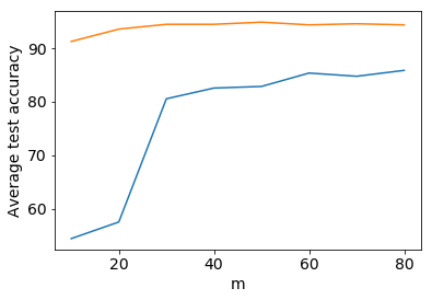
Figure 1: Average test accuracy of GMSA (blue) and DMSA (orange) on the digits dataset as a function of the number of samples used in domain adaptation.

To illustrate the efficiency of DMSA  we further evaluated DMSA and GMSA on the digits dataset when only a small amount of data is available for domain adaptation. We varied $m$, the number of samples per domain and evaluated both DMSA and GMSA, see Figure 1. As expected, DMSA consistently outperforms GMSA, thus matching our theoretical analysis that DMSA can succeed with fewer samples.

Table 2: Digit Dataset Accuracy. DMSA outperforms each single-source domain model, unif, joint, and most importantly GMSA, on various target mixtures.

	Digits Test Data
	svhn	mnist	usps	mu	su	sm	smu	mean
CNN-s	92.3	66.9	65.6	66.7	90.4	85.2	84.2	78.8
CNN-m	15.7	99.2	79.7	96.0	20.3	38.9	41.0	55.8
CNN-u	16.7	62.3	96.6	68.1	22.5	29.4	32.9	46.9
CNN-unif	75.7	91.3	92.2	91.4	76.9	80.0	80.7	84.0
CNN-joint	90.9	99.1	96.0	98.6	91.3	93.2	93.3	94.6
GMSA	91.4	98.8	95.6	98.3	91.7	93.5	93.6	94.7
DMSA (ours)	92.3	99.2	96.6	98.8	92.6	94.2	94.3	95.4

Adult dataset. We also experimented with the UCI adult dataset (Blake, 1998). It contains $32,561$ training samples with numerical and categorical features, each representing a person. The task consists of predicting if the person’s income exceeds $50,000$ dollars. Following (Mohri et al., 2019), we split the dataset into two domains, the doctorate, Doc, domain and non-doctorate, NDoc, domain and used categorical features for training linear classification models. We froze these models and experimented with domain adaptation. Here, we repeatedly sampled $400$ training samples from each domain for training, keeping the test set fixed.

The results are in Table 3. DMSA achieves higher accuracy compared to GMSA on the NDoc domain and also in the average of two domains. The difference in performance is not statistically significant for the Doc domain as it has very few test samples.

Table 3: Linear models for adult dataset. The experiments are averaged over $100$ runs.

Test data	Doc	NDoc	Doc-NDoc
GMSA	70.2 $\pm$ 1.2	76.4 $\pm$ 1.6	73.3 $\pm$ 0.8
DMSA	70.0 $\pm$ 0.8	80.5 $\pm$ 0.5	75.3 $\pm$ 0.4

We finally conducted simulations on a small synthetic dataset to illustrate the difference between GMSA and DMSA. We used the sklearn toolkit for these experiments. Let ${\mathscr{D}}_{1}$ and ${\mathscr{D}}_{2}$ be Gaussian mixtures in one dimensions as follows: ${\mathscr{D}}_{1}=0.9\cdot N(-20,8)+0.1\cdot N(0,0.1)$ and ${\mathscr{D}}_{2}=0.75\cdot N(3,0.1)+0.25\cdot N(5,0.1)+0.05\cdot N(0,0.1)$, see Figure 2. The two domains are similar around $0$ but are disjoint otherwise. Let the labeling function $f(x)=-1\text{ if }x\in[-0.5,0.5]\cup[3.5,\infty)$. The example is designed such that if their estimates are good, then both GMSA and DMSA would achieve close to $100\%$ accuracy. We first sampled $1000$ examples and trained a linear separator $h_{k}$ for each domain $k$. For GMSA, we trained kernel density estimators and chose the bandwidth based on a five-fold cross-validation. For DMSA, we trained a conditional Maxent threshold classifier. We first illustrate the kernel density estimate using $1000$ samples in Figure 2. For $x\in[-0.5,0.5]$, ${\mathscr{D}}_{1}(x)>{\mathscr{D}}_{2}(x)$, but the kernel density estimates satisfy $\widehat{\mathscr{D}}_{2}(x)\geq\widehat{\mathscr{D}}_{1}(x)$, which shows the limitations of kernel density estimation with a single bandwidth. On the other hand, DMSA selected a threshold around $0.3$ for distinguishing between ${\mathscr{D}}_{1}$ and ${\mathscr{D}}_{2}$ and achieves accuracy around $100\%$. We varied the number of examples available for domain adaptation and compared GMSA and DMSA. For simplicity we found the best $z$ using exhaustive search for both GMSA and DMSA. The results show that DMSA consistently outperforms GMSA on both the domains and hence on all convex combinations, see Figure 3. The results also show that DMSA converges quickly in accordance with our theory.

Figure 2: Left: Illustration of the true densities and kernel density estimates for GMSA for domains ${\mathscr{D}}_{1}$ and ${\mathscr{D}}_{2}$ with $1000$ samples. The labeling function $f(x)=-1$ in the green regions and $1$ otherwise. Right: Same estimates zoomed in at $x=0$.

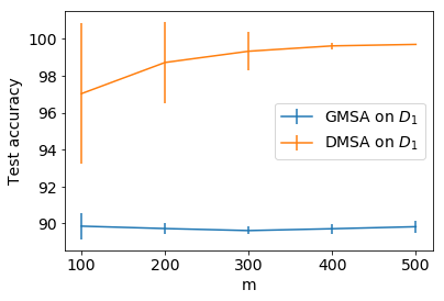
Figure 3: Comparison of GMSA and DMSA on the synthetic dataset. DMSA performs better than GMSA on both the domains and hence on any convex combination. The experiments are averaged over $10$ runs. The error bars show one standard deviation.

6 Conclusion

We presented a new algorithm for the important problem of multiple-source adaptation, which commonly arises in applications. Our algorithm was shown to benefit from favorable theoretical guarantees and a superior empirical performance, compared to previous work. Moreover, our algorithm is practical: it is straightforward to train a multi-class classifier in the setting we described and our DC-programming solution is very efficient.

Providing a robust solution for the problem is particularly important for under-represented groups, whose data is not necessarily well-represented in the classifiers to be combined and trained on source data. Our solution demonstrates improved performance even in the cases where the target distribution is not included in the source distributions. We hope that continued efforts in this area will result in more equitable treatment of under-represented groups.

References

- Arndt (2004) Christoph Arndt. Information Measures: Information and its Description in Science and Engineering. Signals and Communication Technology. Springer Verlag, 2004.
- Blake (1998) Catherine Blake. UCI repository of machine learning databases. https://archive.ics.uci.edu/ml/index.php, 1998.
- Blitzer et al. (2007) John Blitzer, Mark Dredze, and Fernando Pereira. Biographies, bollywood, boom-boxes and blenders: Domain adaptation for sentiment classification. In ACL, pages 440–447, 2007.
- Dredze et al. (2008) Mark Dredze, Koby Crammer, and Fernando Pereira. Confidence-weighted linear classification. In ICML, volume 307, pages 264–271, 2008.
- Ganin et al. (2016) Yaroslav Ganin, Evgeniya Ustinova, Hana Ajakan, Pascal Germain, Hugo Larochelle, François Laviolette, Mario Marchand, and Victor Lempitsky. Domain-adversarial training of neural networks. The Journal of Machine Learning Research, 17(1):2096–2030, 2016.
- Gong et al. (2013a) Boqing Gong, Kristen Grauman, and Fei Sha. Connecting the dots with landmarks: Discriminatively learning domain-invariant features for unsupervised domain adaptation. In ICML, volume 28, pages 222–230, 2013a.
- Gong et al. (2013b) Boqing Gong, Kristen Grauman, and Fei Sha. Reshaping visual datasets for domain adaptation. In NIPS, pages 1286–1294, 2013b.
- Hoffman et al. (2012) Judy Hoffman, Brian Kulis, Trevor Darrell, and Kate Saenko. Discovering latent domains for multisource domain adaptation. In ECCV, volume 7573, pages 702–715, 2012.
- Hoffman et al. (2018) Judy Hoffman, Mehryar Mohri, and Ningshan Zhang. Algorithms and theory for multiple-source adaptation. In Advances in Neural Information Processing Systems, pages 8246–8256, 2018.
- Jacobs et al. (1991) Robert A Jacobs, Michael I Jordan, Steven J Nowlan, and Geoffrey E Hinton. Adaptive mixtures of local experts. Neural computation, 3(1):79–87, 1991.
- Konstantinov and Lampert (2019) Nikola Konstantinov and Christoph Lampert. Robust learning from untrusted sources. In International Conference on Machine Learning, pages 3488–3498, 2019.
- Liao (2013) Hank Liao. Speaker adaptation of context dependent deep neural networks. In ICASSP, pages 7947–7951, 2013.
- Liu et al. (2015) Jianwei Liu, Jiajia Zhou, and Xionglin Luo. Multiple source domain adaptation: A sharper bound using weighted Rademacher complexity. In Technologies and Applications of Artificial Intelligence (TAAI), 2015 Conference on, pages 546–553. IEEE, 2015.
- Mansour et al. (2008) Yishay Mansour, Mehryar Mohri, and Afshin Rostamizadeh. Domain adaptation with multiple sources. In NIPS, pages 1041–1048, 2008.
- Mansour et al. (2009) Yishay Mansour, Mehryar Mohri, and Afshin Rostamizadeh. Multiple source adaptation and the rényi divergence. In Proceedings of UAI, pages 367–374, 2009.
- Mohri et al. (2019) Mehryar Mohri, Gary Sivek, and Ananda Theertha Suresh. Agnostic federated learning. In International Conference on Machine Learning, pages 4615–4625. PMLR, 2019.
- Motiian et al. (2017a) Saeid Motiian, Quinn Jones, Seyed Iranmanesh, and Gianfranco Doretto. Few-shot adversarial domain adaptation. In Advances in Neural Information Processing Systems, pages 6670–6680, 2017a.
- Motiian et al. (2017b) Saeid Motiian, Marco Piccirilli, Donald A Adjeroh, and Gianfranco Doretto. Unified deep supervised domain adaptation and generalization. In Proceedings of the IEEE International Conference on Computer Vision, pages 5715–5725, 2017b.
- Muandet et al. (2013) Krikamol Muandet, David Balduzzi, and Bernhard Schölkopf. Domain generalization via invariant feature representation. In ICML, volume 28, pages 10–18, 2013.
- Nowlan and Hinton (1991) Steven J Nowlan and Geoffrey E Hinton. Evaluation of adaptive mixtures of competing experts. In Advances in neural information processing systems, pages 774–780, 1991.
- Pan and Yang (2010) Sinno Jialin Pan and Qiang Yang. A survey on transfer learning. IEEE Trans. Knowl. Data Eng., 22(10):1345–1359, 2010.
- Saito et al. (2019) Kuniaki Saito, Donghyun Kim, Stan Sclaroff, Trevor Darrell, and Kate Saenko. Semi-supervised domain adaptation via minimax entropy. In Proceedings of the IEEE International Conference on Computer Vision, pages 8050–8058, 2019.
- Sriperumbudur and Lanckriet (2012) Bharath K. Sriperumbudur and Gert R. G. Lanckriet. A proof of convergence of the concave-convex procedure using Zangwill’s theory. Neural Computation, 24(6):1391–1407, 2012.
- Tao and An (1997) Pham Dinh Tao and Le Thi Hoai An. Convex analysis approach to DC programming: theory, algorithms and applications. Acta Mathematica Vietnamica, 22(1):289–355, 1997.
- Tao and An (1998) Pham Dinh Tao and Le Thi Hoai An. A DC optimization algorithm for solving the trust-region subproblem. SIAM Journal on Optimization, 8(2):476–505, 1998.
- Torralba and Efros (2011) Antonio Torralba and Alexei A. Efros. Unbiased look at dataset bias. In CVPR, pages 1521–1528, 2011.
- Tzeng et al. (2015) Eric Tzeng, Judy Hoffman, Trevor Darrell, and Kate Saenko. Simultaneous deep transfer across domains and tasks. In Proceedings of the IEEE International Conference on Computer Vision, pages 4068–4076, 2015.
- Wang et al. (2019a) Boyu Wang, Jorge Mendez, Mingbo Cai, and Eric Eaton. Transfer learning via minimizing the performance gap between domains. In Advances in Neural Information Processing Systems, pages 10645–10655, 2019a.
- Wang et al. (2019b) Tao Wang, Xiaopeng Zhang, Li Yuan, and Jiashi Feng. Few-shot adaptive faster r-cnn. In Proceedings of the IEEE Conference on Computer Vision and Pattern Recognition, pages 7173–7182, 2019b.
- Xu et al. (2018) Ruijia Xu, Ziliang Chen, Wangmeng Zuo, Junjie Yan, and Liang Lin. Deep cocktail network: Multi-source unsupervised domain adaptation with category shift. In Proceedings of the IEEE Conference on Computer Vision and Pattern Recognition, pages 3964–3973, 2018.
- Xu et al. (2014) Zheng Xu, Wen Li, Li Niu, and Dong Xu. Exploiting low-rank structure from latent domains for domain generalization. In ECCV, volume 8691, pages 628–643, 2014.
- Zhang et al. (2015) Kun Zhang, Mingming Gong, and Bernhard Schölkopf. Multi-source domain adaptation: A causal view. In AAAI, pages 3150–3157, 2015.
- Zhao et al. (2018) Han Zhao, Shanghang Zhang, Guanhang Wu, José MF Moura, Joao P Costeira, and Geoffrey J Gordon. Adversarial multiple source domain adaptation. In Advances in neural information processing systems, pages 8559–8570, 2018.