Geodesic stability and Quasi normal modes via Lyapunov exponent for Hayward Black Hole

Abstract

We derive proper-time Lyapunov exponent $(\lambda_{p})$ and coordinate-time Lyapunov exponent $(\lambda_{c})$ for a regular Hayward class of black hole. The proper-time corresponds to $\tau$ and the coordinate time corresponds to $t$. Where $t$ is measured by the asymptotic observers both for for Hayward black hole and for special case of Schwarzschild black hole. We compute their ratio as $\frac{\lambda_{p}}{\lambda_{c}}=\frac{(r_{\sigma}^{3}+2l^{2}m)}{\sqrt{(r_{\sigma}^{2}+2l^{2}m)^{3}-3mr_{\sigma}^{5}}}$ for time-like geodesics. In the limit of $l=0$ that means for Schwarzschild black hole this ratio reduces to $\frac{\lambda_{p}}{\lambda_{c}}=\sqrt{\frac{r_{\sigma}}{(r_{\sigma}-3m)}}$. Using Lyponuov exponent, we investigate the stability and instability of equatorial circular geodesics. By evaluating the Lyapunov exponent, which is the inverse of the instability time-scale, we show that, in the eikonal limit, the real and imaginary parts of quasi-normal modes (QNMs) is specified by the frequency and instability time scale of the null circular geodesics. Furthermore, we discuss the unstable photon sphere and radius of shadow for this class of black hole.

Received (Day Month Year)Revised (Day Month Year)

1 Introduction

An elementary set of unstable circular orbits about a Schwarzschild black hole (BH) are consequences of the non-linearity of general theory of relativity. Their instability could be measured by a positive Lyapunov exponent [1]. Albeit the Lyapunov exponent are often related with chaotic dynamics [2, 3], the geodesics about a Schwarzschild BH are not chaotic; the orbits are completely solvable and hence integrable. The unstable geodesic orbits should have positive Lyapunov exponent [4], which has the invariant properties first established in [5]. Lyapunov exponent has a great impact on general relativity for its numerous applications: they are relative and depend on the coordinate system used, they vary from orbit to orbit. In this work, we are interested to focus on analytical formulation of Lyapunov exponent and QNMs in terms of the expressions of the radial equation of circular geodesics about a BH space-time. In this regard an equatorial circular geodesics about a BH may play crucial role in general theory of relativity for classification of the orbits.

Black holes and singularities are approached to be unavoidable predictions of the theory of general relativity (GR). In order to solve the black hole singularity, several phenomenological propositions have been studied in the existing literatures. Bardeen BH [6] was the first model that has proposed as a spherically symmetric compact object with an event horizon and satisfying the weak energy condition. In the year 2006, Hayward [7] proposed the formation and evaporation of a new kind of regular solution in space-time. The static region of a Hayward space-time is similar to Bardeen black hole. In the article [8] , the authors discussed the massive scalar quasinormal modes of the Hayward black hole. In this study, variations of the Hayward solutions have also been studied as Hayward with charge [9] and Rotating Hayward [10].

The authors in [11, 12, 13] derived the Lyapunov exponent to study the instability for the circular null geodesics in terms of the expressions for QNM of spherically symmetric space-time. Here, the main focus is on the null circular geodesics, which play an important role for the Lyapunov exponent. The null circular geodesics is described by the shortest possible orbital period as estimated by the asymptotic observers [14]. The time circular geodesics provide the slowest way to circle the BH, among all the possible circular geodesics.

The QNMs spectrum for stable BH represents an infinite set of complex frequencies, which designates damped oscillations for the amplitude. It is clear that the oscillations with lower level of damping rate is controlled with slow time, whereas oscillations with higher level of damping rate are exponentially terminated [15]. In 1971, Press [16], first introduced the term ‘quasi-normal frequency’. He showed that when a Schwarzschild BH is perturbed it vibrates with an angular frequency $\omega=\frac{\ell}{\sqrt{27}M}$. Where $M$ is BH mass and $\ell$ is spherical symmetric index. He then interpreted it as vibration frequency of BHs. In the same year the lowest QNMs were computed by investigating test particle falling about Schwarzschild BH. So far the QNMs has been explored substantially in diverse field. The WKB method gives an exact estimation of QNM frequency in the eikonal limit. Also WKB method was first introduced by Schutz and Will [17] to analyze the problem of scattering about BH.

The plan of the ar proper time Lyapunov   exponent $\lambda_{p}$ and coordinate time Lyapunov exponent  $\lambda_{c}$ in terms of second order derivative of the effective potential for the radial motion $\dot{r}^{2}$:

$$\lambda_{p} = \pm\sqrt{\frac{(\dot{r}^{2})^{\prime\prime}}{2}},$$ (1)

$$\lambda_{c} = \pm\sqrt{\frac{(\dot{r}^{2})^{\prime\prime}}{2\dot{t}^{2}}}.$$ (2)

In Sec. 3, we describe the equatorial circular geodesics of spherically symmetric regular Hayward BH. Then we calculate the Lyapunov exponent in terms of the timelike circular geodesics and null circular geodesics. We also discuss the gravitational bending of light and photon sphere for this BH.

In Sec. 4, we derive the relation between QNMs  in the eikonal limit and Lyapunov exponent of a static, spherically symmetric regular Hayward BH. In the limit $l=0$, one obtains the QNMs frequency of spherically-symmetric Schwarzschild BH which was first calculated in [26].

Moreover we compute the angular velocity $\Omega_{c}$ of the unstable null geodesics.   Also, we compute the Lyapunov exponent, which investigates the instability of the time-scale of circular orbit [18, 19, 20]   also which is in agreement with analytic WKB approximations   of QNMs  of the Hayward BH in the eikonal limit. Thus the QNMs frequency in the eikonal limit is found to be

$$\omega_{QNM} = j\,\bigg{(}\frac{\sqrt{m\,(r_{c}^{3}-4m\,l^{2})}}{(r_{c}^{3}+2m\,l^{2})}\bigg{)}-i\left(n+\frac{1}{2}\right)\sqrt{\frac{3m^{2}[r_{c}^{5}-6l^{2}(r_{c}^{3}-2m\,l^{2})]}{(r_{c}^{3}+2m\,l^{2})^{3}}},$$ (3)

where $n$ represents the overtone number and $j$ represents the angular momentum of the perturbation.

For schwarzschild BH, the QNMs frequency becomes

$$\omega_{QNM} = j\sqrt{\frac{m}{r_{c}^{3}}}-i\left(n+\frac{1}{2}\right)\frac{\sqrt{3}m}{r_{c}^{2}}.$$ (4)

The real part of the complex QNM frequency can be determined by the angular velocity of the unstable null geodesics and the imaginary part is related to the instability time scale of the orbit. Finally, we briefly discuss about the outcome of this paper   in Sec. 5.

2 Proper time Lyapunov exponent,  Coordinate time Lyapunov exponent and Geodesic stability

The Lyapunov exponent or Lyapunov characteristic exponent of a dynamical system is a measure of the average rate of expansion and contraction of adjacent trajectories in the phase space. A negative Lyapunov exponent designates the convergence between nearby trajectories. A positive Lyapunov exponent determines the divergence between nearby geodesics in which the path of such a system are the most active to change the starting circumstances. The vanishing Lyapunov exponent designates the existence of marginal stability.   The equation of motion in terms of Lyapunov exponents for geodesic stability analysis should be written as

$$\frac{dZ_{i}}{dt}=F_{i}(Z_{j}),$$ (5)

and its linearized form around a certain orbit is

$$\frac{d\delta Z_{i}(t)}{dt}=A_{ij}(t)\delta Z_{j}(t).$$ (6)

Here,

$$A_{ij}(t)=\frac{\partial F_{i}}{\partial Z_{j}}\Bigg{|}_{Z_{i}(t)},$$ (7)

represents the linear stability matrix [18]. Now, the solution of the Eq. (2) can be written as

$$\delta Z_{i}(t)=X_{ij}(t)\delta Z_{j}(0),$$ (8)

where $X_{ij}(t)$ represents the evolution matrix, which leads to

$$\dot{X}_{ij}(t) = A_{im}X_{mj}(t),$$ (9)

with $X_{ij}(0)=\delta_{ij}$. The principal Lyapunov exponent $\lambda$ can be expressed in terms of the eigenvalues $X_{ij}$ as follows:

$$\lambda = \lim_{t\rightarrow\infty}\frac{1}{t}\log\bigg{(}\frac{X_{ij}(t)}{X_{mj}(0)}\bigg{)}.$$ (10)

If there exists a set of $n$ Lyapunov exponents connected with an n-dimensional independent system, then they can be arranged by the size as

$$\lambda_{1}\geq\lambda_{2}\geq\lambda_{3}\geq,.....,\geq\lambda_{n}.$$ (11)

The set of $n$ numbers of $\lambda_{i}$ are known as Lyapunov spectrum.

In an equatorial plane, for any static spherically symmetric space-time, the Lagrangian of a test particle can be written as

$$\mathcal{L}=\frac{1}{2}\bigg{[}g_{tt}\,\dot{t}^{2}+g_{rr}\,\dot{r}^{2}+g_{\phi\phi}\,\dot{\phi}^{2}\bigg{]}.$$ (12)

From the above expression, the canonical momenta can be derived as

$$p_{q}=\frac{\partial\mathcal{L}}{\partial\dot{q}}.$$ (13)

The generalized momenta derived from the above Lagrangian are

$$p_{t} = g_{tt}\dot{t}=-E=\textrm{Const},$$ (14)

$$p_{\phi} = g_{\phi\phi}\dot{\phi}=L=\textrm{Const},$$ (15)

$$p_{r} = g_{rr}\dot{r}.$$ (16)

Here, ‘dot’ represents the differentiation with respect to proper time $(\tau)$. E and L are the energy and angular momentum per unit rest mass of the test particle, respectively.

Now, from Euler-Lagrange’s equation of motion, we can write

$$\frac{dp_{q}}{d\tau}=\frac{\delta\mathcal{L}}{\delta q}.$$ (17)

Linearizing the above equation of motion in two-dimensional phase space with respect to $Z_{i}(t)=(p_{r},r)$, around the circular orbit (taking $r$ as a constant), we get

$$\frac{dp_{r}}{d\tau}=\frac{\partial\mathcal{L}}{\partial q}~{}~{}~{}~{}\textrm{and}~{}~{}~{}~{}\frac{dr}{d\tau}=\frac{p_{r}}{g_{rr}},$$ (18)

and an infinitesimal evolutionary matrix can be expressed as

$$A_{ij}=\left(\begin{array}[]{cc}0&A_{1}\\ A_{2}&0\\ \end{array}\right),$$ (21)

where

$$A_{1} = \frac{d}{dr}\bigg{(}\dot{t}^{-1}\frac{\delta\mathcal{L}}{\delta r}\bigg{)},$$ (22)

$$A_{2} = -(\dot{t}g_{rr})^{-1}.$$ (23)

For the case of circular orbit, the eigenvalues of the matrix are called principal Lyapunov exponent which can be written as

$$\lambda^{2}=A_{1}A_{2}.$$ (24)

Then the Lagrange’s equation of motion leads to

$$\frac{d}{d\tau}\bigg{(}\frac{\partial\mathcal{L}}{\partial\dot{r}}\bigg{)}-\frac{\partial\mathcal{L}}{\partial r}=0,$$ (25)

and

$$\frac{d}{d\tau}\bigg{(}\frac{\partial\mathcal{L}}{\partial\dot{r}}\bigg{)}=\frac{d}{d\tau}(-g_{rr}\dot{r})=-\dot{r}\frac{d}{dr}(-g_{rr}\dot{r}).$$ (26)

Thus, the Lyapunov exponent in terms of square of radial velocity $\dot{r}^{2}$, can be expressed as

$$\frac{\partial\mathcal{L}}{\partial r} = \frac{d}{dr}(-\dot{r}g_{rr})^{2}$$ (27)

$$= -\frac{1}{2g_{rr}}\frac{d}{dr}(\dot{r}^{2}g_{rr}^{2}).$$

Finally, from (24) and (27), the principal Lyapunov exponent can be written as

$$\lambda^{2}=\frac{1}{2}\frac{1}{g_{rr}}\frac{d}{dr}\bigg{[}\frac{1}{g_{rr}}\frac{d}{dr}(\dot{r}g_{rr})^{2}\bigg{]}.$$ (28)

For the case of circular geodesics [21], we have

$$\dot{r}^{2}=(\dot{r}^{2})^{\prime}=0,$$ (29)

where $\dot{r}^{2}$ is the square of radial potential or effective radial potential. From (28), we can obtain the proper time Lyapunov exponent as

$$\lambda_{p}=\pm\sqrt{\frac{(\dot{r}^{2})^{\prime\prime}}{2}},$$ (30)

and the coordinate time Lyapunov [11] can be derived from (28) as follows

$$\lambda_{c}=\pm\sqrt{\frac{(\dot{r}^{2})^{\prime\prime}}{2\dot{t}^{2}}}.$$ (31)

The above Eqs. (30) and (31) for $\lambda_{p}$ and $\lambda_{c}$ are respectively satisfied for any spherically symmetric BH space-times [22, 24, 23]. Now, we shall drop the $\pm$ sign and consider only positive Lyapunov exponent. The circular orbit is stable when $\lambda$ is imaginary, the circular orbit is unstable when $\lambda$ is real and for $\lambda=0$, the circular orbit becomes marginally stable or saddle point.

Due to Pretorius and Khurana [25], we can define the critical exponent as

$$\gamma=\frac{\Omega}{2\pi\lambda}=\frac{T_{\lambda}}{T_{\Omega}},$$ (32)

where $T_{\lambda}$ represents the Lyapunov time scale, $T_{\Omega}$ represents the orbital time scale and $\Omega$ represent the angular velocity, where $T_{\lambda}=\frac{1}{\lambda}$ and $T_{\Omega}=\frac{2\pi}{\Omega}$. Now, the critical exponent can be written in terms of second order derivative of the square of radial velocity $(\dot{r}^{2})$, as

$$\gamma_{p} = \frac{1}{2\pi}\sqrt{\frac{2\Omega^{2}}{(\dot{r}^{2})^{\prime\prime}}},$$ (33)

$$\gamma_{c} = \frac{1}{2\pi}\sqrt{\frac{2{\dot{\phi^{2}}}}{(\dot{r}^{2})^{\prime\prime}}}.$$ (34)

Here, $\phi$ is an angular coordinate. For circular geodesics $(\dot{r}^{2})^{\prime\prime}>0$, which implies instability. Now, we shall determine the equatorial circular geodesics of Hayward space-time.

3 Equatorial Circular Geodesics in Spherically Symmetric metric Hayward Space-time

In this paper, the metric [7] for a static, spherically symmetric space-time can be taken as follows

$$ds^{2} = -f(r)dt^{2}+\frac{dr^{2}}{f(r)}+r^{2}(d\theta^{2}+\sin^{2}\theta d\phi^{2}),~{}~{}~{}~{}$$ (35)

where

$$f(r)=\bigg{(}1-\frac{2mr^{2}}{r^{3}+2l^{2}m}\bigg{)}.$$ (36)

Here, the parameters $l$ and $m$ are positive constants. This is similar to the Bardeen BH, which can be reduced to the Schwarzschild solution for $l=0$, and become flat space-time for m = 0.

The function $f(r)$ is plotted in Fig. 1. One can observe that the geometry is similar to the Schwarzschild BH with a single horizon. Also there could be a single, double or no horizon which depends on the relation between the parameters. Hayward [7] discussed the formation and evaporation of this new kind of regular and non singular BH where the static region is Bardeen-like and the dynamic regions are Vaidya-like and this inspired scientists to construct a compact star model. This motivates us for considering the regular Hayward black holes. .

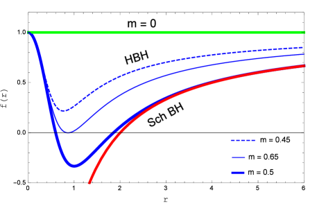
Figure 1: The figure shows the $f(r)$ versus $r$. Here, $l=0.5$ for Hayward BH.

3.1 Circular orbits

To calculate the geodesics in an equatorial plane for space-time of (35), we follow the work of Chandrasekhar [21]. In an equatorial plane, we set $\dot{\theta}=0$ and $\theta=\frac{\pi}{2}$ = constant. Here, we restrict our attention to the equatorial orbits, for which the Lagrangian is given by

$$2\mathcal{L} = \bigg{[}-\bigg{(}1-\frac{2mr^{2}}{r^{3}+2l^{2}m}\bigg{)}\dot{t}^{2}+\frac{\dot{r}^{2}}{\bigg{(}1-\frac{2mr^{2}}{r^{3}+2l^{2}m}\bigg{)}}+r^{2}\dot{\phi}^{2}\bigg{]},$$ (37)

where $\phi$ represents an angular coordinate. By using (13), the generalized momenta can be represented as

$$p_{t} = -\bigg{(}1-\frac{2mr^{2}}{r^{3}+2l^{2}m}\bigg{)}\dot{t}=-E=\textrm{const},$$ (38)

$$p_{\phi} = r^{2}\dot{\phi}=L=\textrm{const},$$ (39)

$$p_{r} = \frac{\dot{r}}{\bigg{(}1-\frac{2mr^{2}}{r^{3}+2l^{2}m}\bigg{)}}.$$ (40)

The Lagrangian is independent on both $t$ and $\phi$, so $p_{t}$ and $p_{\phi}$ are the conserved quantities. Solving Eqs. (38) and (39) for $\dot{t}$ and $\dot{\phi}$, we get

$$\dot{t}=\frac{E}{\bigg{(}1-\frac{2mr^{2}}{r^{3}+2l^{2}m}\bigg{)}}~{}~{}~{}~{}\textrm{and}~{}~{}~{}~{}\dot{\phi}=\frac{L}{r^{2}}.$$ (41)

The normalization of the four velocity vector $(u^{\alpha})$ can be represented as an integral equation for the geodesic motion

$$g_{\alpha\beta}u^{\alpha}u^{\beta}=\xi,$$ (42)

which is equivalent to

$$-E\dot{t}+L\dot{\phi}+\frac{\dot{r}^{2}}{\bigg{(}1-\frac{2mr^{2}}{r^{3}+2l^{2}m}\bigg{)}}=\xi.$$ (43)

Here, $\xi=-1,0,1,$ represents the time-like geodesics, null geodesics and space-like geodesics, respectively. Replacing the values of $\dot{t}$ and $\dot{\phi}$ from (41) in (43), we obtain the radial equation for spherically symmetric space-time:

$$\dot{r}^{2}=E^{2}-\bigg{(}\frac{L^{2}}{r^{2}}-\xi\bigg{)}\bigg{(}1-\frac{2mr^{2}}{r^{3}+2l^{2}m}\bigg{)}.$$ (44)

3.1.1 Time-like geodesics

The radial equation of test particle for time-like circular geodesics [26, 24] is given by

$$\dot{r}^{2} = E^{2}-\bigg{(}1+\frac{L^{2}}{r^{2}}\bigg{)}\bigg{(}1-\frac{2mr^{2}}{r^{3}+2l^{2}m}\bigg{)}.$$ (45)

For circular orbit with constant $r=r_{\sigma}$ and using the condition (29), we get the energy and angular momentum per unit mass of the test particle are

$$E_{\sigma}^{2} = \frac{(r_{\sigma}^{3}+2l^{2}m-2mr_{\sigma}^{2})^{2}}{(r_{\sigma}^{3}+2l^{2}m)^{2}-3mr_{\sigma}^{5}},$$ (46)

$$L_{\sigma}^{2} = \frac{mr_{\sigma}^{4}(r_{\sigma}^{3}-4l^{2}m)}{(r_{\sigma}^{3}+2l^{2}m)^{2}-3mr_{\sigma}^{5}}.$$ (47)

In order to obtain the energy and angular momentum real and finite, the conditions $(r_{\sigma}^{3}+2l^{2}m)^{2}>3mr_{\sigma}^{5}$ and $mr_{\sigma}^{4}(r_{\sigma}^{3}-4l^{2}m)>0$ must be satisfied. Thus the orbital velocity becomes

$$\Omega_{\sigma} = \frac{\dot{\phi}}{\dot{t}}=\frac{\sqrt{m(r_{\sigma}^{3}-4l^{2}m)}}{r_{\sigma}^{3}+2l^{2}m}.$$ (48)

3.1.2 Null geodesics

In case of null geodesics, there is no proper time for photons. Thus, we have to calculate only the coordinate time Lyapunov exponent. The radial equation of the test particle for null circular geodesics is

$$\dot{r}^{2}={V_{ef}}=E^{2}-\frac{L^{2}}{r^{2}}\bigg{(}1-\frac{2mr^{2}}{r^{3}+2l^{2}m}\bigg{)}.$$ (49)

The comparison between the Hayward BH and Schwarzschild BH effective potentials are shown in Fig. 2 for null-circular geodesics. Fig. 2 shows that the effective potential of Hayward BH is smallest compared to Schwarzschild BH.

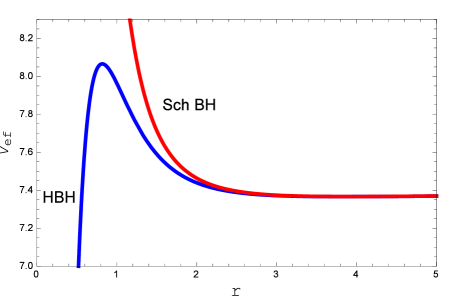
Figure 2: The effective potential $V_{ef}$, for null-circular geodesics in Hayward BH and in Schwarzschild BH is compared. The constants are with $m=1,L=1,E=1$ and for HBH $l=0.5$.

Now, the energy and angular momentum at $r=r_{c}$, for the null geodesics is

$$\frac{E_{c}}{L_{c}}=\pm\sqrt{\frac{(r_{c}^{3}+2l^{2}m-2mr_{c}^{2})}{r_{c}^{2}(r^{3}+2l^{2}m)}}~{}~{}~{}\textrm{and}~{}~{}~{}(r_{c}^{3}+2l^{2}m)^{2}-3mr_{c}^{5}=0.$$ (50)

Let $D_{c}=\frac{L_{c}}{E_{c}}$ be the impact parameter, then the equation (50) reduces to

$$\frac{1}{D_{c}}=\frac{E_{c}}{L_{c}}=\frac{\sqrt{m(r_{c}^{3}-4l^{2}m)}}{(r_{c}^{3}+2l^{2}m)}=\Omega_{c}=\frac{\dot{\phi}}{\dot{t}}.$$ (51)

3.2 Bending of light

A unstable circular photon orbit is called “Photon Sphere”. The unstable photon sphere constitutes the shadow of the BH. From Eq. (39) and Eq. (40) we find

$$\frac{dr}{d\phi}=\frac{\dot{r}}{\dot{\phi}}=\frac{p_{r}\bigg{(}1-\frac{2mr^{2}}{r^{3}+2l^{2}m}\bigg{)}r^{2}}{L}.$$ (52)

Again the Eq. (49) can be written as

$$p_{r}^{2}\bigg{(}1-\frac{2mr^{2}}{r^{3}+2l^{2}m}\bigg{)}=\frac{E^{2}}{(1-\frac{2mr^{2}}{r^{3}+2l^{2}m})}-\frac{L^{2}}{r^{2}}.$$ (53)

We can obtain $p_{r}$ from above equation as

$$p_{r}=\pm\sqrt{\frac{1}{(1-\frac{2mr^{2}}{r^{3}+2l^{2}m})}}\sqrt{\frac{E^{2}}{(1-\frac{2mr^{2}}{r^{3}+2l^{2}m})}-\frac{L^{2}}{r^{2}}}.$$ (54)

Using $p_{r}$ from Eq. (54), we can write the Eq. (52) as follows

$$\frac{dr}{d\phi}=\pm\sqrt{r^{2}\,\bigg{(}1-\frac{2mr^{2}}{r^{3}+2l^{2}m}\bigg{)}}\sqrt{\frac{E^{2}}{L^{2}}\chi^{2}(r)-1},$$ (55)

where,

$$\chi^{2}(r)=\frac{r^{2}}{\left(1-\frac{2mr^{2}}{r^{3}+2l^{2}m}\right)}$$ (56)

A light ray which comes in from infinity, reaches at minimum radius $R$ and again goes back to infinity, the bending angle $(\beta_{bending})$ is given by the formula

$$\beta_{bending}=-\pi+2\int_{R}^{\infty}\frac{dr}{\sqrt{r^{2}\bigg{(}1-\frac{2mr^{2}}{r^{3}+2l^{2}m}\bigg{)}\bigg{(}\frac{E^{2}}{L^{2}}\chi^{2}(r)-1\bigg{)}}}$$ (57)

Since $R$ is the turning point of the trajectory, the condition $\frac{dr}{d\phi}|_{R=0}$ must be hold. Which implies the following equation

$$\chi^{2}(R)=\frac{L^{2}}{E^{2}}.$$ (58)

Then the deflection angle can be written in terms of $R$ as

$$\beta_{bending}=-\pi+2\int_{R}^{\infty}\frac{dr}{\sqrt{r^{2}\bigg{(}1-\frac{2mr^{2}}{r^{3}+2l^{2}m}\bigg{)}\bigg{(}\frac{\chi^{2}(r)}{\chi^{2}(R)}-1\bigg{)}}}$$ (59)

After putting the value of $\chi^{2}(r)$ and $\chi^{2}(R)$, the equation of bending angle of Hayward BH is

$$\beta_{bending}=-\pi+2\int_{R}^{\infty}\frac{dr}{\sqrt{r^{2}\bigg{(}1-\frac{2mr^{2}}{r^{3}+2l^{2}m}\bigg{)}\bigg{(}\frac{r^{2}}{D^{2}\left(1-\frac{2mr^{2}}{r^{3}+2l^{2}m}\right)}-1\bigg{)}}}$$ (60)

where, $D=\frac{L}{E}$ is the impact parameter of the Hayward BH. The exact formula of bending angle is derived in [37] .

3.2.1 Radius of the Shadow

A circular light orbits corresponds to zero velocity and acceleration, so that $\dot{r}=0$ and $\ddot{r}=0$ , implies that $p_{r}=0$ and $\dot{p_{r}}=0$. From  Eq. (53) we obtain

$$\frac{E^{2}}{(1-\frac{2mr^{2}}{r^{3}+2l^{2}m})}-\frac{L^{2}}{r^{2}}=0$$ (61)

Now differentiating Eq. (53) with respect to affine parameter and putting the value of $p_{r}=0$ and $\dot{p_{r}}=0$ we have

$$\frac{E^{2}(8m^{2}l^{2}r-2mr^{4})}{(r^{3}+2l^{2}m-2mr^{2})^{2}}+\frac{2L^{2}}{r^{3}}=0$$ (62)

From equations (61) and (62) we have

$$L^{2}=\frac{r^{2}E^{2}(r^{3}+2l^{2}m)}{(r^{3}+2l^{2}m-2mr^{2})}=\frac{r^{3}E^{2}(2mr^{4}-8m^{2}l^{2}r)}{2(r^{3}+2l^{2}m-2mr^{2})^{2}}$$ (63)

Subtracting these two equations and after some simplification we can obtain an equation for radius of the circular light orbit in the following form

$$\frac{d}{dr}\chi^{2}(r)=0$$ (64)

Hence, from Eq. (64), the equation of photon sphere is at $r=r_{c}$

$$r_{c}^{6}-3m\,r_{c}^{5}+4m\,l^{2}\,r_{c}^{3}+4m^{2}\,l^{4} = 0$$ (65)

Let $r_{ps}=r_{c}$ be the real root of the equation then $r_{ps}$ is the radius of circular photon sphere [37]. Let $R$ be the critical value of the minimum radius. Then we can write $R$ in terms of $r_{ps}$ as follows

$$R=\frac{r_{ps}^{2}(r^{3}_{ps}+2l^{2}m)}{(r^{3}_{ps}+2l^{2}m-2mr_{ps}^{2})}$$ (66)

Here, we consider a light ray which is send from the observer’s position at $r_{c}$ into the past under an angle $\beta$ with respect to the radial direction. Therefore, we have

$$\cot\beta=\frac{1}{\sqrt{r^{2}\bigg{(}1-\frac{2mr^{2}}{r^{3}+2l^{2}m}\bigg{)}}}\frac{dr}{d\phi}|_{R=0}$$ (67)

Again from Eq. (55) we have

$$\frac{dr}{d\phi}=\pm\sqrt{r^{2}\bigg{(}1-\frac{2mr^{2}}{r^{3}+2l^{2}m}\bigg{)}}\sqrt{\frac{\chi^{2}(r)}{\chi^{2}(R)}-1}.$$ (68)

For the angle $\beta$ we have

$$\cot^{2}\beta=\frac{\chi^{2}(r_{c})}{\chi^{2}(R)}-1,$$ (69)

and

$$\sin^{2}\beta=\frac{\chi^{2}(R)}{\chi^{2}(r_{c})}=\frac{D^{2}_{c}(r^{3}_{c}+2l^{2}m-2mr^{2}_{c})}{r_{c}^{2}(r^{3}_{c}+2l^{2}m)}.$$ (70)

The boundary of Shadow $\beta_{shadow}$ is described by light rays which spiral asymptotically towards a circular light orbit at radius $r_{ps}$. Then the angular radius of the shadow is given by

$$\sin^{2}\beta_{shadow}=\frac{\chi^{2}(r_{ps})}{\chi^{2}(r_{c})}=\frac{r^{2}_{ps}(r^{3}_{ps}+2l^{2}m-2mr^{2}_{ps})(r^{3}_{c}+2l^{2}m)}{r_{c}^{2}(r^{3}_{c}+2l^{2}m-2mr^{2}_{c})(r^{3}_{ps}+2l^{2}m)},$$ (71)

where $r_{ps}$ has to be determined from the equation (65).

3.3 Lyapunov exponent

3.3.1 Time-like case

Using Eqs. (30) and (31), the proper time Lyapunov exponent and coordinate time Lyapunov exponent becomes

$$\lambda_{p} = \sqrt{\frac{-m\left[r_{\sigma}^{5}(r_{\sigma}-6m)+22m\,l^{2}\,r_{\sigma}^{3}-32l^{4}\,m^{2}\right]}{(r_{\sigma}^{3}+2l^{2}\,m)\left[(r_{\sigma}^{3}+2m\,l^{2})^{2}-3m\,r_{\sigma}^{5}\right]}},$$ (72)

$$\lambda_{c} = \sqrt{\frac{-m\left(r_{\sigma}^{5}(r_{\sigma}-6m)+22m\,l^{2}\,r_{\sigma}^{3}-32\,l^{4}\,m^{2}\right)}{\left(r_{\sigma}^{3}+2m\,l^{2}\right)^{3}}}.$$ (73)

The time-like circular geodesics is stable when $r_{\sigma}^{5}(r_{\sigma}-6m)+22l^{2}mr_{\sigma}^{3}-32l^{4}m^{2}>0$, that is, $\lambda_{p}$ and $\lambda_{c}$ become imaginary. The time-like circular geodesics is unstable when $r_{\sigma}^{5}(r_{\sigma}-6m)+22l^{2}mr_{\sigma}^{3}-32l^{4}m^{2}<0$, that is, $\lambda_{p}$ and $\lambda_{c}$ become real and the time-like circular geodesics is marginally stable when $r_{\sigma}^{5}\,(r_{\sigma}-6m)+22m\,l^{2}\,r_{\sigma}^{3}-32l^{4}\,m^{2}=0$, that is, $\lambda_{p}$ and $\lambda_{c}$ becomes zero.

Now one can analyze the equation $r_{\sigma}^{6}-6m\,r_{\sigma}^{5}+22m\,l^{2}\,r_{\sigma}^{3}-32l^{4}\,m^{2}=0$ which gives us the radii of innermost stable circular orbit. Since it is a non-trivial equation. One can determine its root numerically for various values of $l$. For example if we choose the value of $l=1$ then one obtains the ISCO radius at $r_{isco}=5.19m$. For $l=2$, we find ISCO radius is at $r_{isco}=1.91m$.

The ratio of proper time Lyapunov exponent and coordinate time Lyapunov exponent is

$$\frac{\lambda_{p}}{\lambda_{c}}=\frac{(r_{\sigma}^{3}+2l^{2}m)}{\sqrt{(r_{\sigma}^{3}+2l^{2}m)^{2}-3mr_{\sigma}^{5}}}.$$ (74)

One could see the variation of $\frac{\lambda_{p}}{\lambda_{c}}$ in graphically (See Fig. 3) for Hayward BH.

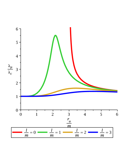
Figure 3: The variation of $\frac{\lambda_{p}}{\lambda_{c}}$ with $\frac{r_{\sigma}}{m}$ for Hayward BH.

It can be easily seen from above Fig.3 that, the ratio of $\lambda_{p}$ and $\lambda_{c}$ varies from orbit to orbit for various values of $\frac{l}{m}$. Also, Fig.3 shows that the ratio $\frac{\lambda_{p}}{\lambda_{c}}$ of Hayward BH is smallest compared to Schwarzschild ($\frac{l}{m}=0$) BH.

Therefore, the reciprocal of critical exponent is given by

$$\frac{1}{\gamma_{p}}=\frac{T_{\Omega}}{T_{\lambda}}=2\pi\sqrt{\frac{-\left[r_{\sigma}^{5}\,(r_{\sigma}-6m)+22m\,l^{2}\,r_{\sigma}^{3}-32l^{4}m^{2}\right](r_{\sigma}^{3}+2l^{2}m)}{(r_{\sigma}^{3}-4l^{2}m)\left[(r_{\sigma}^{3}+2l^{2}m)^{2}-3mr_{\sigma}^{5}\right]}}.$$ (75)

Special case:

For Schwarzschild BH $l=0$, the proper time Lyapunov exponent and coordinate time Lyapunov exponent are given by

$$\lambda_{p}^{Sch}=\sqrt{\frac{-m(r_{\sigma}-6m)}{r_{\sigma}^{3}(r_{\sigma}-3m)}},$$ (76)

$$\lambda_{c}^{Sch}=\sqrt{\frac{-m(r_{\sigma}-6m)}{r_{\sigma}^{4}}}.$$ (77)

The ratio of $\frac{\lambda_{p}}{\lambda_{c}}$ reduces to

$$\frac{\lambda_{p}}{\lambda_{c}} = \sqrt{\frac{r_{\sigma}}{(r_{\sigma}-3m)}}.$$ (78)

The reciprocal of critical exponent for schwarzschild BH is given by

$$\frac{1}{\gamma_{p}}=\frac{T_{\Omega}}{T_{\lambda}}=2\pi\sqrt{\frac{-(r_{\sigma}-6m)}{(r_{\sigma}-3m)}}.$$ (79)

When $r_{\sigma}=4m$, the circular orbit become unstable and critical exponent $(\gamma_{p})$ become $\frac{1}{2\sqrt{2}\pi}$. In this case, Lyapunov time scale $T_{\lambda}=\frac{1}{\lambda}$ will be less than the orbital time scale $T_{\Omega}=\frac{2\pi}{\Omega}$, that is, $T_{\lambda}<T_{\Omega}$ in the approximation of a test particle around a Schwarzschild BH.

3.3.2 Null geodesics

By using Eq. (31) the Lyapunov exponent for null geodesics is given by

$$\lambda_{c}=\sqrt{\frac{3m^{2}\left[r_{c}^{5}-6l^{2}(r_{c}^{3}-2l^{2}m)\right]}{(r_{c}^{3}+2l^{2}m)^{3}}}.$$ (80)

Here we can see that the circular geodesics is unstable as $\lambda_{c}$ is real.

Special case:

For Schwarzschild BH $l=0$, the Lyapunov exponent becomes

$$\lambda_{c}^{Sch}={\frac{\sqrt{3}m}{r_{c}^{2}}}.$$ (81)

It can be easily seen that for $r_{c}=3m$; $\lambda_{c}^{Sch}$ is real which implies that Schwarzschild photon sphere is unstable.

4 Null Circular Geodesic and QNMs for Hayward BH in the Eikonal limit

We consider the usual wave like equation, with an effective potential which was first derived by Iyer and Will [27],

$$\frac{d^{2}Y}{dr_{*}^{2}}+\Psi_{0}Y=0,$$ (82)

where,

$$\Psi_{0} = w^{2}-V_{s}(r)$$ (83)

and

$$V_{s}(r) = \bigg{[}\frac{j(j+1)}{r^{2}}+\frac{2m(r^{3}-4l^{2}m)}{(r^{3}+2l^{2}m)^{2}}\bigg{]}\bigg{(}1-\frac{2mr^{2}}{r^{3}+2l^{2}m}\bigg{)}$$ (84)

Here,where $j$ being the angular harmonic index, $Y$ represents the radial part of the perturbation variable and $r_{*}$ is a convenient “tortoise” coordinate, ranging from $-\infty$ to $+\infty$.

The radial coordinate $r$ and the tortoise coordinate $r_{*}$ are related by the following equation

$$\frac{dr}{dr_{*}} = 1-\frac{2mr^{2}}{r^{3}+2l^{2}m}.$$ (85)

In case of the eikonal limit $(j\rightarrow\infty)$, we get

$$\Psi_{0}\simeq\omega^{2}-\frac{{j^{2}}}{r^{2}}\bigg{(}1-\frac{2mr^{2}}{r^{3}+2l^{2}m}\bigg{)}.$$ (86)

With the help of Eq. (86), we can find the maximum value of $\Psi_{0}$ which occurs at $r=r_{o}$

$$(r_{o}^{3}+2l^{2}m)^{2}-3mr_{o}^{5}=0.$$ (87)

Also from the null circular geodesic at $r=r_{c}$ , we obtain

$$(r_{c}^{3}+2l^{2}m)^{2}-3mr_{c}^{5}=0.$$ (88)

Since the location of the null circular geodesics and the maximum value of $\Psi_{0}$ are coincident at $r_{c}=r_{o}$, then we get the following QNM condition [28, 29]

$$\frac{\Psi_{0}(r_{o})}{\sqrt{-2\Psi_{0}^{{}^{\prime\prime}}(r_{o})}}=i(n+1/2),$$ (89)

where $\Psi_{0}^{{}^{\prime\prime}}\equiv\frac{d^{2}\Psi_{0}}{dr_{*}^{2}}$ and Eq. (89) is evaluated at an extremum of $\Psi_{0}$ (the point $r_{0}$ at which $\frac{d\Psi_{0}}{dr_{*}}=0$).

Now, the formula (89) allows us to conclude that, in case of the large-$j$ limit

$$\omega_{QNM}=j\bigg{(}\frac{\sqrt{m(r_{c}^{3}-4l^{2}m)}}{(r_{c}^{3}+2l^{2}m)}\bigg{)}-i\left(n+\frac{1}{2}\right)\sqrt{\frac{3m^{2}\left[r_{c}^{5}-6l^{2}(r_{c}^{3}-2l^{2}\,m)\right]}{(r_{c}^{3}+2l^{2}m)^{3}}}.$$ (90)

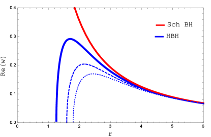
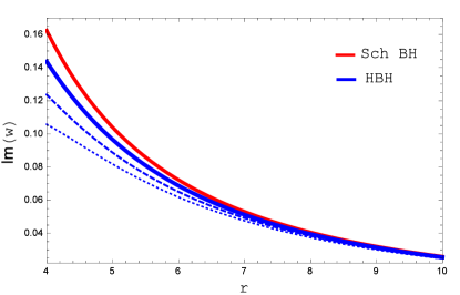
Figure 4: The figure shows QNMs frequency $Re(w)$ versus $r$ (left Panel) and $Im(w)$ versus $r$ (right panel) of HBH and Sch BH ; the other parameters fixed to $m=1$ and $l=0.7(\textrm{solid}),l=1(\textrm{dashed})$ and $l=1.2(\textrm{dotted})$ for HBH.

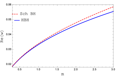
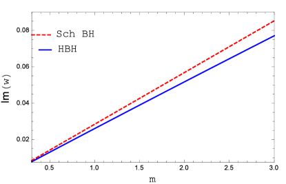
Figure 5: The figure shows QNMs frequency $Re(w)$ versus $m$ (left Panel) and $Im(w)$ versus $m$ (right panel) of HBH and Sch BH ; the other parameter fixed to $l=0.5$ for HBH.

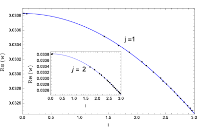
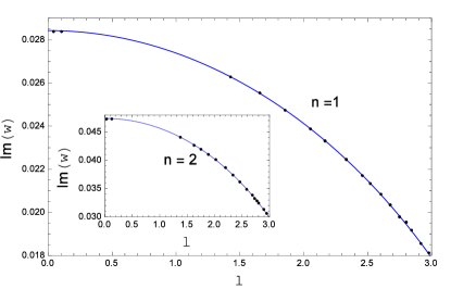
Figure 6: The figure shows QNMs frequency $Re(w)$ versus $l$ (left Panel) and $Im(w)$ versus $l$ (right panel) of Hayward BH; the other parameter fixed to $m=1$ .

Cardoso et al. [11] showed in general sense that this is one of the most important results of QNMs and the significance of the Eq. (90) is that in case of eikonal limit [30], the real and imaginary parts of the QNMs [33, 32, 36, 31] of the spherically symmetric, asymptotically flat Hayward regular BH space-time are given by the frequency and instability time scale of the unstable null circular geodesics.

Special case:

For Schwarzschild BH l = 0, in case of eikonal limit the frequency of QNM is given by

$$\omega_{QNM}=j\,\sqrt{\frac{m}{r_{c}^{3}}}-i\left(n+\frac{1}{2}\right)\frac{\sqrt{3}m}{r_{c}^{2}}.$$ (91)

Hence, by determining the Lyapunov exponent, we established that in case of eikonal limit, the frequency of quasi-normal modes of Schwarzschild BH might be determined by the parameters of the null circular geodesics.

In Fig.4, Re(w) is plotted as a function of $r$ (left panel) by varying $l$. When $l$ increase, the height of the $Re(w)$ decrease. Also $Im(w)$ is plotted as a function of $r$ (right panel) by varying $l$. One can observe that $Im(w)$ decreases when $r$ increases and $Im(w)$ of Hayward BH is the smallest compared to Schwarzschild BH.

The Fig.5, shows that the behavior is similar for Hayward BH and Schwarzschild BH in both cases $Re(w)$ and $Im(w)$ increase when $m$ is increase, respectively. In fact $Im(w)$ is linearly dependent on $m$. Also, the angular velocity and instability time scale of null-circular geodesics of Hayward BH is the smallest compared to Schwarzschild BH regardless of the value of mass, respectively.

In Fig.6, $Re(w)$ is plotted against $l$ (left panel) and $Im(w)$ is plotted against $l$ (right panel). Both of $Re(w)$ and $Im(w)$ are decrease when $l$ increases, that is, the modes decays faster for large $l$. Compared to the Schwarzschild BH ($l=0$) the modes decays faster.

5 Conclusions

We investigated the geodesic stability via Lyapunov exponent for a static, spherically symmetric regular Hayward BH. We have considered both time-like case and null case. Using Lyapunov exponent one can easily determined whether the geodesics is stable or unstable or marginally stable. Also, we computed the QNMs frequency in the geometric-optics approximation (eikonal) limit. We have showed that the real part of QNMs frequency are evaluated by the angular velocity in terms of the unstable circular photon orbit. While the imaginary part is related to the instability time scale of photon orbit.

Moreover, we examined the Lyapunov exponent that could be used to established the instability of equatorial circular geodesics both for time-like and null cases. When the parameter $l=0$, one gets the result of Schwarzschild BH. We derived both the proper time Lyapunov exponent and coordinate time Lyapunov exponent. We have calculated their ratio. We have also calculated the reciprocal of critical exponent. Moreover, we have showed that for any unstable circular orbit, $T_{\Omega}>T_{\lambda}$, that is, orbital time scale is greater than the Lyapunov time scale.

The most important result that we derived is the relation between unstable null circular geodesics and QNMs frequency in the eikonal limit. Moreover we discussed the gravitational bending of light and radius of shadow for this regular BH.

Conflict of interest

The authors declare that they have no conflict of interest.

References

- [1] N. J. Cornish, Phys. Rev D, 64 084011 (2001)
- [2] A.E. Motter, Phys. Rev. Lett. 91 231101 (2003).
- [3] J.R. Dorfman, An Introduction to Chaos in Non equilibrium Statistical Mechanics (Cambridge University Press, Cambridge, 1999); H. A. Posh and W. G. Hoover, J. Phys.: Conf. Ser. 31, 9 (2006).
- [4] Lyapunov, A.M.: The General Problem of the Stability of Motion, Taylor and Francis, London (1992).
- [5] V. Karas, D. Vokrouhlicky, Gen. Relativ. Gravit 24 729 (1992).
- [6] J.M. Bardeen, in: Conference Proceedings of GR5, Tbilisi, USSR p.174. (1968)
- [7] S.A.Hayward, Phys. Rev. Lett. 96 031103 (2006), arXiv:gr-qc/0506126.
- [8] K. Lin, J. Li, S. Yang, Int. J. Theor. Phys. 52 3771 (2013).
- [9] Valeri P. Frolov. Notes on nonsingular models of black holes. Phys. Rev. D 94(10):104056 (2016)
- [10] Muhammed Amir and Sushant G. Ghosh. Rotating Hayward?s regular black hole as particle accelerator. JHEP, 07:015, (2015).
- [11] V. Cardoso, A. S. Miranda, E. Berti, H. Witek, V. T. Zanchin, Phys. Rev. D 79 064016 (2009).
- [12] V. Cardoso, J. P. S. Lemos, Phys. Rev. D 67 084020.
- [13] U. Sperhake, V. Cardoso , F. Pretorius, E. Berti, J.A. Gonzalez Phys. Rev. Lett. 101 161101 (2008).
- [14] S. Hod, Phys. Rev. D 84 104024 (2011).
- [15] R. A. Konoplya, Rev. Mod. phys 83 793 (2011).
- [16] W. H. Press, Astrophys. J. 170 L105L108 (1971).
- [17] B. F. Schutz, C. M. Will, Astrophys. J. 291 L33 (1985).
- [18] N. Cornish, Levin, Class. Quant. Grav. 20 1649 (2003).
- [19] L. Bombelli ,E. Calzetta, Class. Quant. Grav. 9 2573 (1992).
- [20] T. Manna, F. Rahaman, M. Mondal, Modern Physics Letters A 2050034 (2019).
- [21] S. Chandrasekhar, The Mathematical Theory of Black Holes, ( Oxford University Press, New York, 1983).
- [22] P. Pradhan, P. Majumdar, Physics Letters A 375 474-479 (2011).
- [23] M. R. Setare, D. Momeni, Int J Theor Phys 50 106-113 (2011).
- [24] D. Pugliese, H. Quevedo, R. Ruffini, Phys. Rev. D 83 024021 (2011).
- [25] F.Pretorius, D. Khurana, Class. Quant. Grav. 24 S83 (2007)
- [26] P.Pradhan, Pramana 87, 5 (2016).
- [27] S. Iyer, C. M. Will,Phys. Rev. D 35 3621 (1987).
- [28] S. Iyer, Phys. Rev. D 35 3632 (1987).
- [29] E. Berti, V. Cardoso, J. A. Gonzalez, U. Sperhake, M. Hannam, S. Husa, B. Brugmann, Phys. Rev. D 76 064034 (2007).
- [30] J.G.Baker, W.D.Boggs, J.Centrella, B.J. Kelly, S. T. McWilliams, J. R. V. Meter, Phys. Rev. D 78 044046 (2008).
- [31] F. R.T angherlini, Nuovo Cim. 27 636 (1963).
- [32] H. P. Nollert, Class. Quant. grav. 16 R159 (1999).
- [33] K. D.Kokkotas, B. Schmidt, Living Rev. Relativity 2 2 (1999).
- [34] S. W. Wei, Y.X. Liu, Phys. Rev D 89 047502 (2014).
- [35] I.Z.Stefanov, S.S.Yazadjiev, G.G.Gyulchev, Phys. Rev. Lett. 104:251103 (2010).
- [36] A. K. Yadav, M. Mondal, F. Rahaman, arXiv:2004.07956v1 [gr-gc].
- [37] T. Chiba, M. Kimura, Prog. Theor. Exp. Phys., 043E01, (2017)
- [38] S. H. Hendi, A. Nemati, arXiv:1912.06824 [gr-qc].
- [39] R. A. Konoplya and Z. Stuchl k, Phys. Lett.B 771, 597 (2017)
- [40] B. Toshmatov, Z. Stuchl k, B. Ahmedov, and D. Malafarina, Phys. Rev.D, 99, 064043 (2019)
- [41] Z. Stuchl k and J. Schee, Eur. Phys. J. C, 79, 44 (2019)
- [42] J. Schee and Z. Stuchl k, J. Cosmol. Astropart. Phys., 06 048 (2015). P. Pradhan, arXiv:1402.2748