Quantum versus thermal fluctuations in the harmonic chain and experimental implications

Abstract

The nonzero ground-state energy of the quantum mechanical harmonic oscillator implies quantum fluctuations around the minimum of the potential with the mean square value proportional to Planck’s constant. In classical mechanics thermal fluctuations occur when the oscillator is coupled to a heat bath of temperature $T$. At finite temperature quantum statistical mechanics allows the description of the transition from pure quantum fluctuations at $T=0$ to classical thermal fluctuations in the high temperature limit. It was early pointed out by Peierls that the mean square thermal fluctuations in a harmonic chain increase linearly with the distance of the atoms in the chain, destroying long range crystalline order. The corresponding pure quantum fluctuations lead to a much slower logarithmic increase with the distance from the fixed end of the chain. It is also shown that this implies, fo example, the absence of sharp Bragg peaks in x-ray scattering in an infinite chain at zero temperature, which instead show power law behaviour typical for one dimensional quantum liquids (called Luttinger liquids).

I Introduction

This paper addresses the question “what are quantum fluctuations, how do they differ from classical thermal fluctuations and what are measurable consequences?”. In order to simplify the discussion a single particle in a one dimensional external potential is treated before switching to one of the simplest many-body systems, the harmonic chain.

Despite the fact that quantum mechanics and quantum statistical mechanics are used in this paper we start with a short discussion in the framework of classical physics. In classical mechanics a particle of mass $m$ moving in a time independent external potential $V(x)$ has a well defined “ground state” if the potential is everywhere larger than its value at a single (non degenerate) mimimum. The typical example is the harmonic oscillator

$$V(x)=\frac{\lambda}{2}x^{2}=\frac{1}{2}m\omega_{0}^{2}x^{2}$$ (1)

where the particle at rest at the origin corresponds to the ground state. Thermal fluctuations around this position occur if the particle is coupled to a heat bath described by a canonical ensemble. Then the probability distribution to find the particle at position $x$ is given by $w_{T,cl}(x)\sim\exp(-\beta V(x))$, where $\beta=1/(k_{B}T)$ with $k_{B}$ the Boltzmann constant and $T$ the temperature of the bath Huang . The moments $\langle x^{n}\rangle_{T,cl}\equiv\int x^{n}w_{T,cl}(x)dx$ for $n=1,2$ describe the fluctuations around the minimum. As $w$ is an even function $\langle x\rangle_{T,cl}$ vanishes and $\langle x^{2}\rangle_{T,cl}$ directly gives the mean square deviation. In order to obtain $\langle x^{2}\rangle_{T,cl}$ one can either use the fact that a Gaussian probability distribution has the form $w_{G}(x)\sim\exp(-x^{2}/(2\langle x^{2}\rangle))$ or one can use the equipartition theorem of classical statistical mechanics Huang $\langle V\rangle_{T,cl}=k_{B}T/2$ which holds for the quadratic oscillator potential, i.e.

$$\langle x^{2}\rangle_{T,cl}=\frac{k_{B}T}{\lambda}=\frac{k_{B}T}{m\omega^{2}_{0}}\equiv\sigma^{2}_{cl}~{}.$$ (2)

Now we switch to quantum mechanics. The Hamiltonian $\hat{H}$ usually depends on operators $\hat{A},\hat{B},...$ which do not commute. A simple example is a particle in an external potential

$$\hat{H}=\frac{\hat{p}^{2}}{2m}+V(\hat{x})~{},$$ (3)

where the commutation relation $[\hat{x},\hat{p}]=i\hbar\hat{1}$ leads to the uncertainty relation Baym

$$\Delta\hat{x}\Delta\hat{p}\geq\hbar/2~{}.$$ (4)

Here $\Delta\hat{A}\equiv\sqrt{\langle\hat{A}^{2}\rangle_{\Phi}-\langle\hat{A}\rangle^{2}_{\Phi}}$ with $\langle\hat{A}^{n}\rangle_{\Phi}\equiv\langle\Phi|\hat{A}^{n}|\Phi\rangle$ and $|\Phi\rangle$ is the quantum state of the system.

For the harmonic oscillator the uncertainty relation implies quantum fluctuations even in the ground state $|0\rangle$, usually called “zero point motion”. The corresponding probability distribution $w_{0}(x)$ is again Gaussian with vanishing $\langle\hat{x}\rangle_{0}$ (see next section). The mean square fluctuations can be obtained without the explicit form of ground state wavefunction using the virial theorem Merzb . For the eigenstates of the harmonic oscillator it states the equality of the expectation value of the kinetic energy and the potential energy. With the ground state energy $\epsilon_{0}=\hbar\omega_{0}/2$ this implies

$$\langle\hat{x}^{2}\rangle_{0}=\frac{\hbar}{2m\omega_{0}}\equiv\sigma^{2}_{qm}~{}.$$ (5)

In section II we dicuss how the results for the classical thermal fluctuation Eq. (2) and the quantum fluctuation Eq. (5) connect as a function of temperature. Messiah . This discussion is extended to the harmonic chain in section III. In the classical ground state of the chain the $n$-th atom is located at the lattice position $na$ if atom number zero is fixed at the origin. Here $a$ is the lattice constant. It was pointed out early by Peierls Peierls in the classical context that while $\langle x_{n}\rangle_{cl}=na$ holds also at finite temperatures, thermal fluctuations destroy long range order at any finite temperature as the mean square deviations $\langle(x_{n+l}-x_{l}-na)^{2}\rangle$ of the separations of two atoms diverge linearly with $n$ and proportional to the temperature $T$. Therefore crystalline order exists classically only at zero temperature. It is discussed in section III how quantum fluctuations destroy crystalline order even at $T=0$ by a much weaker logarithmic divergence with $n$. It is again discussed how the results for the results for the classical thermal fluctuations and the pure quantum fluctuations connect as a function of temperature. It turns out that the different dependence on the frequency in Eqs. (2) and (5) plays a decisive role.

In the context of harmonic lattices in two dimensions, a similar logarithmic divergence occurs in the calculation of classical thermal fluctuations.Jancovici ; MS The main results presented here for the harmonic chain, including the power law shape of the Bragg peaks, cannot be found in the literature.

II The harmonic oscillator

As a warm-up to analyzing the harmonic chain, we first discuss both the quantum fluctuations and the thermal fluctuations of a single harmonic oscillator. Our treatment uses the ladder operators that are introduced in almost every textbook. Baym ; Merzb ; Messiah

II.1 Ground state properties

The Hamiltonian of a one-dimensional harmonic oscillator reads

$$\hat{H}=\frac{1}{2m}\hat{p}^{2}+\frac{\lambda}{2}\hat{x}^{2},$$ (6)

where $m$ is the mass of the particle and $\lambda$ the spring constant. With the frequency $\omega_{0}=\sqrt{\lambda/m}$ one defines the lowering operator $\hat{a}$ and its adjoint $\hat{a}^{\dagger}$

$$\hat{a}=\sqrt{\frac{m\omega_{0}}{2\hbar}}\hat{x}+\frac{i}{\sqrt{2m\hbar\omega_{0}}}\hat{p}~{};~{}~{}\hat{a}^{\dagger}=\sqrt{\frac{m\omega_{0}}{2\hbar}}\hat{x}-\frac{i}{\sqrt{2m\hbar\omega_{0}}}\hat{p}~{},$$ (7)

which obey the commutation relation $[\hat{a},\hat{a}^{\dagger}]=\hat{1}$. The position operator $\hat{x}$ and the momentum operator $\hat{p}$ read in terms of $a$ and $\hat{a}^{\dagger}$

$$\hat{x}=\sqrt{\frac{\hbar}{2m\omega_{0}}}\left(\hat{a}+\hat{a}^{\dagger}\right);~{}~{}\hat{p}=-i\sqrt{\frac{m\hbar\omega_{0}}{2}}\left(\hat{a}-\hat{a}^{\dagger}\right).$$ (8)

The Hamiltonian $\hat{H}$, then takes the form

$$\hat{H}=\hbar\omega_{0}\left(\hat{a}^{\dagger}\hat{a}+\frac{1}{2}\right)$$ (9)

and its eigenstates $|n\rangle$ and eigenvalues are given by

$$|n\rangle=\frac{(\hat{a}^{\dagger})^{n}}{\sqrt{n!}}|0\rangle~{};~{}~{}\epsilon_{n}=\hbar\omega_{0}\left(n+\frac{1}{2}\right).$$ (10)

The ground state $|0\rangle$ is annihilated by $\hat{a}$, i.e. $\hat{a}|0\rangle=0$ holds. In the position representation $\langle x|\hat{a}|0\rangle=0$ is a linear differential equation which determines the ground state wavefunctionBaym

$$\phi_{0}(x)\equiv\langle x|0\rangle=\left(\frac{m\omega_{0}}{\pi\hbar}\right)^{1/4}\exp{\left(-\frac{m\omega_{0}}{2\hbar}x^{2}\right)}~{}.$$ (11)

In order to calculate ground state expectation values of functions of $\hat{x}$ and $\hat{p}$ one can either use the explicit form of $\phi_{0}(x)$ or the property $\hat{a}|0\rangle=0$ only. As an example we consider the operator $\exp{(-ik\hat{x})}$. Its expectation value is readily calculated in the position representation. It is given by the Fourier transform of $|\phi_{0}(x)|^{2}$ which is obtained by a Gaussian integration. Alternatively one can use Eq. (8) and the Baker-Haussdorff(BH) formula Merzb which will be used also for the harmonic chain. This formula reads

$$e^{\hat{A}+\hat{B}}=e^{\hat{A}}e^{\hat{B}}e^{-\frac{1}{2}[\hat{A},\hat{B}]},~{}~{}\mbox{if}~{}~{}[\hat{A},[\hat{A},\hat{B}]]=0=[\hat{B},[\hat{A},\hat{B}]].$$ (12)

For operators $\hat{A}$ and $\hat{B}$ linear in the ladder operators the requirements are fulfilled. With $v\equiv-ik\sqrt{\hbar/(2m\omega_{0})}$ one obtains

$$\langle 0|e^{-ik\hat{x}}|0\rangle = \langle 0|e^{v\hat{a}^{\dagger}+v\hat{a}}|0\rangle$$ (13)

$$= \langle 0|e^{v\hat{a}^{\dagger}}e^{v\hat{a}}|0\rangle e^{-\frac{1}{2}v^{2}[\hat{a}^{\dagger},\hat{a}]}$$

$$= \exp{\left(-\frac{\hbar k^{2}}{4m\omega_{0}}\right)}~{}.$$

Because of $\hat{a}|0\rangle=0$ which implies $\langle 0|\hat{a}^{\dagger}=0$ the expectation value in the second equality equals $1$. As a test we recover the ground state density $w_{0}(x)$ which is obtained much more simply by squaring $\phi_{0}(x)$. The operator $\hat{\rho}(x)$ of the particle density can be written as an operator valued Dirac delta function

$$\hat{\rho}(x) = |x\rangle\langle x|=\int dx^{\prime}|x^{\prime}\rangle\langle x^{\prime}|\delta(x-x^{\prime})$$ (14)

$$\equiv \delta(x-\hat{x})~{}.$$

Using the representation of the Dirac delta function as a Fourier integral one has to perform a Gaussian integration

$$w_{0}(x) = \langle 0|\delta(x-\hat{x})|0\rangle=\frac{1}{2\pi}\int_{-\infty}^{\infty}e^{ikx}\langle 0|e^{-ik\hat{x}}|0\rangle dk$$ (15)

$$= \left(\frac{m\omega_{0}}{\pi\hbar}\right)^{1/2}\exp{\left(-\frac{m\omega_{0}}{\hbar}x^{2}\right)}~{}.$$

For finite temperatures the corresponding calculation is simpler than via the position representation.

Because of $[\hat{a},\hat{H}]=\omega_{0}\hat{a}$ the time dependence of the lowering operator $\hat{a}$ in the Heisenberg picture takes the simple form Baym

$$\hat{a}(t)=e^{i\hat{H}t/\hbar}\hat{a}e^{-i\hat{H}t/\hbar}=\hat{a}e^{-i\omega_{0}t}~{}.$$ (16)

II.2 Finite temperature properties

We consider the harmonic oscillator in thermal equilibrium described by the canonical ensemble with temperature $T$. As discussed in textbooks on statistical mechanics Huang the expectation value of an observable $A$ in thermal equilibrium is given by

$$\langle\hat{A}\rangle=\frac{\mbox{Tr}(\hat{A}e^{-\beta\hat{H}})}{\mbox{Tr}(e^{-\beta\hat{H}})}=\frac{1}{Z}\sum_{n}\langle E_{n}|\hat{A}|E_{n}\rangle e^{-\beta E_{n}},$$ (17)

where $\beta=1/(k_{B}T)$, the $|E_{n}\rangle$ are the eigenstates of the Hamiltonian and $Z=\mbox{Tr}(e^{-\beta\hat{H}})=\sum_{n}e^{-\beta E_{n}}$ is the partition function.

It is useful to consider expectation values of an important class of operators, $(\hat{a}^{\dagger})^{l}\hat{a}^{n}$, where $l$ and $n$ are integers. As only diagonal matrix elements contribute in Eq. (17) the thermal expectation values $\langle(\hat{a}^{\dagger})^{l}\hat{a}^{n}\rangle$ vanish unless $l=n$. We therefore calculate the expectation values of the operators $\hat{A}_{n}\equiv(\hat{a}^{\dagger})^{n}\hat{a}^{n}$

$$\langle\hat{A}_{n}\rangle = \frac{1}{Z}\mbox{Tr}\left((\hat{a}^{\dagger})^{n}\hat{a}^{n}e^{-\beta\hat{H}}\right)$$ (18)

$$= \frac{1}{Z}\mbox{Tr}\left((\hat{a}^{\dagger})^{n}\hat{a}^{n-1}e^{-\beta\hat{H}}e^{\beta\hat{H}}\hat{a}e^{-\beta\hat{H}}\right)$$

$$= \frac{1}{Z}\mbox{Tr}\left((\hat{a}^{\dagger})^{n}\hat{a}^{n-1}e^{-\beta\hat{H}}\hat{a}e^{-\beta\hbar\omega_{0}}\right)$$

$$= e^{-\beta\hbar\omega_{0}}\frac{1}{Z}\mbox{Tr}\left(\hat{a}(\hat{a}^{\dagger})^{n}\hat{a}^{n-1}e^{-\beta\hat{H}}\right).$$

In the third line the result $\hat{a}e^{-\beta\hbar\omega_{0}}$ for the Heisenberg operator with imaginary argument $\hat{a}(-i\beta\hbar)$ was inserted and in the last equality the cyclic invariance of the trace was used. Next, the $\hat{a}$ on the left of creation operators is moved back to the right. With the operator identity

$$\hat{a}(\hat{a}^{\dagger})^{n}=[\hat{a},(\hat{a}^{\dagger})^{n}]+(\hat{a}^{\dagger})^{n}\hat{a}=n(\hat{a}^{\dagger})^{n-1}+(\hat{a}^{\dagger})^{n}\hat{a}$$ (19)

valid for $n\geq 1$, Eq. (18) goes over to the recursion relation

$$\langle\hat{A}_{n}\rangle = e^{-\beta\hbar\omega_{0}}\left(n\langle\hat{A}_{n-1}\rangle+\langle\hat{A}_{n}\rangle\right)$$ (20)

$$= \frac{n}{e^{\beta\hbar\omega_{0}}-1}\langle\hat{A}_{n-1}\rangle$$

for $n\geq 1$. With the trivial starting point $\langle\hat{A}_{0}\rangle=1$ one obtains for $n=1$ the well known result

$$\langle\hat{a}^{\dagger}\hat{a}\rangle=\frac{1}{e^{\beta\hbar\omega_{0}}-1}\equiv n_{B}(\omega_{0}),$$ (21)

where $n_{B}$ is the Bose function. This result can be obtained more directly using the thermodynamic relation $\langle\hat{H}\rangle=-\partial\log{Z}/\partial\beta$. For general $n>1$ one obtains Wick’s theorem FW for the harmonic oscillator

$$\langle(\hat{a}^{\dagger})^{n}\hat{a}^{m}\rangle=\delta_{nm}n!\langle\hat{a}^{\dagger}\hat{a}\rangle^{n}.$$ (22)

Generalizations of Wick’s theorem play an important role in quantum field theory.

Wick’s theorem, Eq. (22), can be used to obtain the relation

$$\langle e^{\lambda\hat{a}^{\dagger}}e^{\mu\hat{a}}\rangle = \sum_{n=0}^{\infty}\sum_{m=0}^{\infty}\frac{\lambda^{n}\mu^{m}}{n!m!}\langle(\hat{a}^{\dagger})^{n}\hat{a}^{m}\rangle=\sum_{n=0}^{\infty}\frac{(\lambda\mu)^{n}}{n!}\langle\hat{a}^{\dagger}\hat{a}\rangle^{n}$$ (23)

$$= e^{\lambda\mu\langle\hat{a}^{\dagger}\hat{a}\rangle}=e^{\lambda\mu n_{B}(\omega_{0})}~{}.$$

which is used frequently in the following. Operator products like those on the lhs of Eqs. (22) and (23) are called “normal ordered” because all lowering operators, in the field theoretical context called annihilation operators, are to the right of the creation operators $\hat{a}^{\dagger}$. Products like $(\lambda\hat{a}^{\dagger}+\mu\hat{a})^{2}$ are not normal ordered. In the calculation of expectation values of operators of this type one uses the commutation relation $[\hat{a},\hat{a}^{\dagger}]=\hat{1}$ for normal ordering

$$\langle(\lambda\hat{a}^{\dagger}+\mu\hat{a})^{2}\rangle = \langle\lambda^{2}(\hat{a}^{\dagger})^{2}+\lambda\mu(\hat{a}^{\dagger}\hat{a}+\hat{a}\hat{a}^{\dagger})+\mu^{2}\hat{a}^{2}\rangle$$ (24)

$$= \lambda\mu(1+2n_{B}),$$

which yields the important identityMermin

$$\langle e^{\lambda\hat{a}^{\dagger}+\mu\hat{a}}\rangle=\langle e^{\lambda\hat{a}^{\dagger}}e^{\mu\hat{a}}\rangle e^{-[\lambda\hat{a}^{\dagger},\mu\hat{a}]/2}=e^{\langle(\lambda\hat{a}^{\dagger}+\mu\hat{a})^{2}\rangle/2},$$ (25)

where we have used the BH-identity as well as Eqs. (23) and (24).

With this identity one can immediately generalize the calculation of the average density in Eq. (15) using $\langle\exp{(ik\hat{x})}\rangle=\exp{(-k^{2}\langle\hat{x}^{2}\rangle/2)}$. This implies that the average density is Gaussian for all temperatures

$$\langle\delta(x-\hat{x})\rangle=\frac{1}{\sqrt{2\pi\langle\hat{x}^{2}\rangle}}\exp{\left(-\frac{x^{2}}{2\langle\hat{x}^{2}\rangle}\right)},$$ (26)

with

$$\langle\hat{x}^{2}\rangle=\frac{\hbar}{2m\omega_{0}}\left[1+2n_{B}(\omega_{0})\right].$$ (27)

This derivation of the result for the average density at arbitrary temperature is much shorter than the one presented in Ref. 4. At $T=0$ the Bose function $n_{B}(\omega_{0})$ vanishes and one obtains the ground state result Eq.(5). In the high temperature limit $\epsilon\equiv\hbar\omega_{0}/k_{B}T\ll 1$ one obtains $1+2n_{B}(\omega_{0})=1+2(\epsilon+\epsilon^{2}/2+...)^{-1}=2k_{B}T/\hbar\omega_{0}+O(\epsilon)$ and $\langle\hat{x}^{2}\rangle$ goes over to the classical result Eq. (2). The crossover from the pure quantum fluctuations at $T=0$ to the classical thermal fluctuations is shown in Fig. 1. At any nonzero temperature quantum and thermal fluctuations cannot be disentangled, but for $k_{B}T/\hbar\omega_{0}\ll 1$ the fluctuations are “quantum dominated” and for $k_{B}T/\hbar\omega_{0}\gg 1$ they are almost like classical thermal fluctuations.

The generalization of Eq. (27) to the case of the harmonic chain plays an important role in the next section.

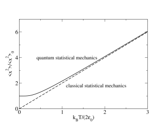
Figure 1: Mean square deviation $\langle\hat{x}^{2}\rangle$ scaled by the ground state value of the harmonic oscillator as function of the scaled temperature $k_{B}T/(\hbar\omega_{0})$.

Using the BH-identity the relation $\langle e^{\hat{A}}\rangle=e^{\langle\hat{A}^{2}\rangle/2}$ of Eq. (25) is easily generalized to

$$\langle e^{\hat{A}}\ e^{\hat{B}}\rangle=e^{(\langle\hat{A}^{2}+\hat{B}^{2}+2\hat{A}\hat{B}\rangle)/2}$$ (28)

for any operators $\hat{A}$ and $\hat{B}$ that are linear in the ladder operators.

III The harmonic chain

We now apply the same principles to a harmonic chain: a one-dimensional chain of $N$ coupled harmonic oscillators (e.g. masses connected by springs). This system is often discussed in classical mechanics courses, because it allows a complete analytical solution. In solid state physics books the harmonic chain usually serves as an introduction to chapters on lattice dynamics of solids AM . The interaction between atoms consists of a short range repulsive and a long range attractive interaction resulting in a two-body interaction potential with a deep minimum. Therefore the atoms are assumed to be confined to their wells and are treated as distinguishable, i.e. the fact whether the atoms are fermions or bosons does not enter the description. In the harmonic approximation the atoms are assumed to perform small oscillations around these minima which leads to linear equations of motion. For low temperatures $T$ quantum effects are important resulting in the Debye law $\sim T^{d}$ for the specific heat, where $d$ is the spatial dimension of the lattice AM . It was pointed out early by Peierls in the classical context that fluctuations have drastic effects for $d\leq 2$, like the loss of long range order Peierls ; Jancovici ; MS . Here we discuss the harmonic chain ($d=1$) in the framework of quantum statistical mechanics.

An exact analytical calculation of correlation functions like the static structure factor AM which appears in the theoretical description of X-ray scattering is possible for the harmonic chain using the operator identities introduced in the context of the harmonic oscillator. Power law behaviour emerges in limiting regions. Similar power laws show up for interacting fermions in one dimension. This is called “Luttinger liquid” behaviour Tomonaga ; Luttinger ; Haldane ; SM .

III.1 Normal modes and ladder operators

In most textbooks chains with periodic boundary conditions are discussed corresponding to particles on a ring AM . For the discussion of the quantum fluctuations it is more convenient to “pin” one end of the chain (“sample holder”). For a chain of equal masses $m$ and spring constants $\lambda$ the Hamiltonian $\hat{H}=\hat{T}+\hat{V}$ reads

$$\hat{H}=\sum_{i=1}^{N}\frac{\hat{p}_{i}^{2}}{2m}+\frac{\lambda}{2}\left[(\hat{x}_{1}-a)^{2}+\sum_{i=1}^{N-1}(\hat{x}_{i+1}-\hat{x}_{i}-a)^{2}\right]$$ (29)

when the left end of the chain is pinned to the origin by a harmonic force of the same strength as the interparticle force . Here $a$ is the separation at which the two-body interaction has its minimum. The potential $V$ vanishes when the $\hat{x}_{n}$ are replaced by the classical ground state positions $na$. If one introduces the displacement operators

$$\hat{u}_{n}\equiv\hat{x}_{n}-na$$ (30)

the operator of the potential energy reads

$$\hat{V}=\frac{\lambda}{2}\left[\hat{u}_{1}^{2}+\sum_{i=1}^{N-1}(\hat{u}_{i+1}-\hat{u}_{i})^{2}\right]\equiv\frac{\lambda}{2}\sum_{n,m}C_{nm}\hat{u}_{n}\hat{u}_{m}~{},$$ (31)

where the last equality defines the matrix ${\bf C}$. In order to obtain the normal modes for this equal mass chain one solves the eigenvalue problem

$${\bf C}{\bf\xi}^{(j)}=C_{j}{\bf\xi}^{(j)}~{}.$$ (32)

and expands the displacement operators $\hat{u}_{n}$ into normal modes $\hat{U}_{j}$ as in the classical case

$$\hat{u}_{n}=\sum_{j=1}^{N}\hat{U}_{j}\xi_{n}^{(j)}~{};~{}~{}~{}~{}~{}\hat{U}_{j}=\sum_{n=1}^{N}\xi_{n}^{(j)}\hat{u}_{n}~{}.$$ (33)

The components $\xi_{n}^{(j)}$ of the orthonormal eigenvectors ${\bf\xi}^{(j)}$ of the real symmetric eigenvalue problem Eq. (32) are chosen real. With the corresponding normal momentum operators $\hat{P}_{j}=\sum_{n=1}^{N}\xi_{n}^{(j)}\hat{p}_{n}$ the Hamiltonian takes the form

$$\hat{H}=\sum_{j=1}^{N}\left[\frac{\hat{P}_{j}}{2m}+\frac{\lambda}{2}C_{j}\hat{U}_{j}^{2}\right]$$ (34)

and $[\hat{U}_{i},\hat{P}_{j}]=i\hbar\delta_{ij}$ holds. In the normal mode basis the system looks like a system of independent harmonic oscillators with eigenfrequencies given by

$$\omega_{j}^{2}=\frac{\lambda}{m}C_{j}\equiv\omega^{2}_{s}C_{j}~{},$$ (35)

where the index “s” indicates the case of a single oscillator (in the previous section $\omega_{s}$ was labeled $\omega_{0}$).

The explicit form of the matrix ${\bf C}$ can be read off Eq. (31). The equations for the components $\xi_{n}^{(j)}$ of the eigenvector ${\bf\xi}^{(j)}$ read for $2\leq n\leq N-1$

$$2\xi_{n}^{(j)}-\xi_{n-1}^{(j)}-\xi_{n+1}^{(j)}=C_{j}\xi_{n}^{(j)}$$ (36)

and the two boundary equations are given by

$$2\xi_{1}^{(j)}-\xi_{2}^{(j)}=C_{j}\xi_{1}^{(j)},~{}~{}~{}\xi_{N}^{(j)}-\xi_{N-1}^{(j)}=C_{j}\xi_{N}^{(j)}~{}.$$ (37)

These equations can be solved with the ansatz

$$\xi_{n}^{(j)}=\xi_{n}(\tilde{k}_{j})\sim\mbox{Re}[e^{i(\tilde{k}_{j}n+\phi_{j})}],$$ (38)

where the $\tilde{k}_{j}$ and $\phi_{j}$ are dimensionless real numbers and “Re” denotes the real part. We formally use this ansatz also for $n=0$ and $n=N+1$. It is shown below that conditions on the $\xi_{n}(\tilde{k}_{j})$ at the boundaries can be formulated such that the two boundary equations take the same form as Eq. (36). Therefore the eigenvalues of ${\bf C}$ follow from the ansatz as

$$C_{j}=2(1-\cos\tilde{k}_{j})=4\sin^{2}(\tilde{k}_{j}/2)$$ (39)

and the $N$ allowed values for $\tilde{k}_{j}$ are determined by the conditions from the boundary equations.

The boundary equation Eq. (37) at the left end of the chain takes the “bulk form” Eq. (36) if one subtracts $\xi_{0}(\tilde{k}_{j})$ on the lhs imposing

$$\xi_{0}(\tilde{k}_{j})=0~{}.$$ (40)

This condition is usually called “fixed boundary condition” (fbc). In order for the eigenvector component to obey this condition one has to to take $\phi_{j}=\pi/2$ in the ansatz, i.e.

$$\xi_{n}(\tilde{k}_{j})\sim\sin(\tilde{k}_{j}n)~{}.$$ (41)

The allowed $\tilde{k}_{j}$-values follow from the boundary equation at the right end of the chain Eq. (37) . It takes the bulk form Eq. (36) by adding $\xi_{N}(\tilde{k}_{j})-\xi_{N+1}(\tilde{k}_{j})$ on the lhs imposing

$$\xi_{N}(\tilde{k}_{j})=\xi_{N+1}(\tilde{k}_{j}).$$ (42)

This is called “open boundary condition” (obc). Using $\sin[\tilde{k}_{j}(N+1)]-\sin(\tilde{k}_{j}N)=2\cos[\tilde{k}_{j}(N+1/2)]\sin(\tilde{k}_{j}/2)$ one obtains the allowed values of $\tilde{k}_{j}$ and the corresponding (squared) eigenfrequencies as

$$\tilde{k}_{j}=\frac{j-1/2}{N+1/2}~{}\pi~{};~{}~{}~{}~{}~{}~{}\omega^{2}_{j}=4\omega^{2}_{s}\sin^{2}(\tilde{k}_{j}/2)~{},$$ (43)

where $j=1,...,N$. The corresponding normalized eigenvectors are given by

$$\xi_{n}^{(j)}=\sqrt{\frac{2}{N+1/2}}~{}\sin(\tilde{k}_{j}n)\equiv A_{N}\sin(\tilde{k}_{j}n)~{}.$$ (44)

The normalization constant $A_{N}$ is obtained using $\sum_{n=1}^{N}\cos(2\tilde{k}_{j}n)=Re\left(\sum_{n=1}^{N}e^{i2\tilde{k}_{j}n}\right)$ and evaluating the geometric series.

In the long wave limit $0<\tilde{k}_{j}\ll 1$ the eigenfrequencies $\omega_{j}=\omega_{s}C_{j}$ depend linearly on the $\tilde{k}_{j}$

$$\omega_{j}=2\omega_{s}\sin(\tilde{k}_{j}/2)\equiv\frac{2c}{a}\sin(ak_{j}/2)\approx ck_{j}.$$ (45)

Here $c=a\omega_{s}$ is the sound velocity and the $k_{j}\equiv\tilde{k}_{j}/a$ are the wave numbers. This “low energy behaviour” is responsible for the divergences of the correlations in the limit $N\to\infty$ studied in the next section. These divergences do not occur if each atom moves in an additional harmonic potential of strength $\lambda_{loc}>0$ centered at its lattice position. It is a simple exercise to show that the corresponding eigenfrequencies are given by $(\lambda_{loc}/m+4\omega^{2}_{s}\sin^{2}(\tilde{k}_{j}/2))^{1/2}$ and stay finite for $\tilde{k}_{j}\to 0$. Except for the discussion in the outlook we keep $\lambda_{loc}=0$ in the following calculations.

As $\omega_{j}^{2}>0$ holds for all eigenfrequencies one can introduce ladder operators as for the case of a single oscillator

$$\hat{a}_{j}=\sqrt{\frac{m\omega_{j}}{2\hbar}}~{}\hat{U}_{j}+\frac{i}{\sqrt{2m\hbar\omega_{j}}}\hat{P}_{j}$$ (46)

and the corresponding $\hat{a}_{j}^{\dagger}$ which obey the commutation relations

$$[\hat{a}_{i},\hat{a}_{j}^{\dagger}]=\delta_{ij}\hat{1}~{},~{}~{}~{}[\hat{a}_{i},\hat{a}_{j}]=0~{}.$$ (47)

Expressed in terms of these ladder operators the Hamiltonian reads

$$\hat{H}=\sum_{j=1}^{N}\left[\hbar\omega_{j}\left(\hat{a}_{j}^{\dagger}\hat{a}_{j}+1/2\right)\right]\equiv\sum_{j=1}^{N}\hat{H}_{j}~{}.$$ (48)

Because of the factorization $e^{-\beta\hat{H}}=\prod_{j=1}^{N}e^{-\beta\hat{H}_{j}}$ the operator relations derived for a single harmonic oscillator can easily be generalized to the harmonic chain.

III.2 Static correlation functions

In terms of the ladder operators of the eigenmodes the operators for the displacements read

$$\hat{u}_{n}=\sum_{j}\sqrt{\frac{\hbar}{2m\omega_{j}}}(\hat{a}_{j}+\hat{a}_{j}^{\dagger})\xi_{n}^{(j)}~{}.$$ (49)

The averages $\langle\hat{u}_{n}\rangle$ vanish, i.e. the average positions $\langle\hat{x}_{n}\rangle=na$ are given by the classical $T=0$ result. Using $\langle a_{j}^{\dagger}\hat{a}_{i}\rangle=\delta_{ij}\langle a_{i}^{\dagger}\hat{a}_{i}\rangle$ one obtains the mean square displacements of the particle positions as

$$\langle\hat{u}_{n}^{2}\rangle=\sum_{j}\frac{\hbar}{2m\omega_{j}}\left[1+2n_{B}(\omega_{j})\right](\xi_{n}^{(j)})^{2}.$$ (50)

As in the introduction we start the discussion with the classical limit $k_{B}T\gg\hbar\omega_{s}$ implying $1+2n_{B}(\omega_{j})\to 2k_{B}T/\hbar\omega_{j}$, for all frequencies $\omega_{j}$, i.e.

$$\langle u_{n}^{2}\rangle_{cl}=k_{B}T\sum_{j}\frac{(\xi_{n}^{(j)})^{2}}{m\omega_{j}^{2}}=\frac{k_{B}T}{m\omega_{s}^{2}}({\bf C}^{-1})_{nn}~{}.$$ (51)

One can either use the explicit form of the eigenfrequencies Eq. (43) and the eigenvector components Eq. (44) to obtain the mean square fluctuations or calculate $({\bf C}^{-1})_{nn}$ directly. The inverse matrix ${\bf C}^{-1}$ can be obtained by a simple observation. The application of ${\bf C}$ to an arbitrary vector ${\bf b}$ can be read off the lhs of Eqs. (36) and (37). For ${\bf b}^{T}_{n}=(1,2,...n-1,n,n,....n)$ one obtains ${\bf Cb}_{n}={\bf e}_{n}$ where ${\bf e}_{n}$ is the $n$-th unit vector. Therefore ${\bf b}_{n}$ is the $n$-th column of ${\bf C}^{-1}$. The diagonal elements are given by $({\bf C}^{-1})_{nn}=n$. Using the sound velocity $c=\omega_{s}a$ this leads to

$$\langle(x_{n}-na)^{2}\rangle_{cl}/a^{2}=\frac{k_{B}T}{mc^{2}}n\equiv\eta_{cl}n$$ (52)

in the classical limit. Here we compare the fluctuations to the squared lattice distance and introduced the dimensionless temperature variable $\eta_{cl}$, which is independent of quantum properties. In order for the harmonic approximation to be applicable $\langle u_{1}^{2}\rangle_{cl}$ should be much smaller than $a^{2}$, i.e. $\eta_{cl}\ll 1$ should hold.

It provides additional insight to consider also the $j$-sum on the rhs of Eq. (51) which is proportional to $\sum_{j}\sin^{2}(\tilde{k}_{j}n)/(4\sin^{2}(\tilde{k}_{j}/2))$. Except for small $n$ the sum is dominated by the $0<\tilde{k}_{j}\ll 1$ contributions. Therefore working in the numerical evaluation with the linearized dispersion, i.e. $2\sin(\tilde{k}_{j}/2)\to\tilde{k}_{j}$, only leads to a small shift compared to the exact result. This can be seen explicitely in the infinite-chain limit $N\to\infty$. In this limit sums of functions of $\tilde{k}_{j}$ go over to integrals $A_{N}^{2}\sum_{j}F(\tilde{k}_{j})\to(2/\pi)\int F(\tilde{k})d\tilde{k}$. Using the linearized dispersion one obtains for $n>0$

$$\langle u^{2}_{n}\rangle_{cl}/a^{2} \approx \frac{2\eta_{cl}}{\pi}\int_{0}^{\pi}\frac{\sin^{2}(\tilde{k}n)}{\tilde{k}^{2}}d\tilde{k}$$

$$= \frac{2\eta_{cl}}{\pi}n\left[\int_{0}^{\infty}\frac{\sin^{2}u}{u^{2}}du-\int_{n\pi}^{\infty}\frac{\sin^{2}u}{u^{2}}du\right]$$

$$\approx \eta_{cl}\left(n-\frac{1}{\pi^{2}}\right)~{}.$$

The integral from $0$ to $\infty$ can be found in tables. In the integral from $n\pi$ to $\infty$ one only makes a small error by replacing $\sin^{2}u$ by its average value $1/2$ if $n$ is sufficiently large. The additional term $-\eta_{cl}/\pi^{2}$ explains the small deviation obtained in the numerical evaluation for a finite chain length.

The deviation $\langle(x_{n}-na)^{2}\rangle_{cl}$ from the lattice position $na$ increases with $n$ without bound in the infinite chain limit. Therefore no crystalline order exists in the classical description at finite temperatures.

The explicit form of ${\bf C}^{-1}$ also leads to $\langle(u_{n}-u_{l})^{2}\rangle_{cl}=\sigma^{2}_{cl}|n-l|$, used later.

We next consider the quantum fluctuations in the ground state. In order to compare the fluctuations to the lattice constant we introduce the $\hbar$-dependent quantum mechanical dimensionless ratio

$$\alpha\equiv\frac{\hbar}{mac}=2\frac{\sigma_{qm}^{2}}{a^{2}}~{}.$$ (54)

If one takes experimental values of three-dimensional crystals in the typical rangeAM $c=4\cdot 10^{3}$m/sec, $a=4\cdot 10^{-10}$m and $m=Am_{\rm proton}$ with $A$ the nucleon number one obtains $\alpha\approx 0.04/A$. In order for the harmonic approximation to be valid the ground state fluctuations of a single particle should be small compared to $a$ which implies $\alpha\ll 1$, fulfilled for not too light elements.

Only the dimensionless ratio $\eta$ defined as

$$\eta\equiv\frac{\eta_{cl}}{\alpha}=\frac{k_{B}T}{\hbar\omega_{s}}$$ (55)

is allowed to be larger than one.

One obtains the ground state quantum fluctuations by putting $n_{B}=0$ in Eq. (50). Dividing by $a^{2}$ this yields

$$\langle\hat{u}_{n}^{2}\rangle_{0}/a^{2}=\frac{\alpha}{N+1/2}\sum_{j=1}^{N}\frac{\sin^{2}(\tilde{k}_{j}n)}{2\sin(\tilde{k}_{j}/2)}~{}.$$ (56)

The numerical evaluation of the sum as a function of $n$ is shown in Fig. 2 for $N=950$ and $N=1000$.

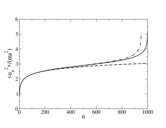
Figure 2: Quantum fluctuations $\langle\hat{u}_{n}^{2}\rangle$ scaled by $\alpha a^{2}$ for $N=1000$ (full curve) and $N=950$ (dashed-dotted curve) as a function of the distance from the fixed left end of the chain. The dashed line shows the logarithmic increase $\log n/(2\pi)+\rm{const.}$ discussed in the text.

Again the sum is dominated by the $0<\tilde{k}_{j}\ll 1$ contributions and therefore working in the numerical evaluation with the linearized dispersion, i.e. $2\sin(\tilde{k}_{j}/2)\to\tilde{k}_{j}$ again only leads to a small shift ($\approx 0.07$) for $\langle u_{n}^{2}\rangle_{cl}/\sigma^{2}_{qm}$ compared to the result with the exact dispersion. The increase with $n$ is much slower than the linear increase in the classical limit. For $n<N/3$ the increase can be well approximated by $const.+(1/\pi)\log n$, i.e. the quantum fluctuations lead to a logarithmic increase. This can be seen analytically in the infinite chain limit

$$\langle\hat{u}_{n}^{2}\rangle_{0}/a^{2} \approx \frac{\alpha}{\pi}\int_{0}^{\pi}\frac{\sin^{2}(\tilde{k}n)}{\tilde{k}}d\tilde{k}$$

$$= \frac{\alpha}{\pi}\left[\int_{0}^{b}\frac{\sin^{2}u}{u}du+\int_{b}^{n\pi}\frac{\sin^{2}u}{u}du\right]$$

$$\approx \alpha\left({\rm const.}+\frac{1}{2\pi}\log n\right)~{},$$

where in the integral from $b(\approx 1)$ to $n\pi$ we again replaced $\sin^{2}u$ by its average value $1/2$. In conjunction with the small value of $\alpha$ the slow logarithmic increase of the fluctuations implies that the long range order due to the quantum fluctuations is destroyed only in very long chains with $N\gg e^{\pi/\alpha}$. A good way to visualize this is to consider the ground-state density. Its operator is given by

$$\hat{\rho}(x) = \sum_{n=1}^{N}\delta(x-\hat{x}_{n})$$

$$= \int_{-\infty}^{\infty}\frac{dk}{2\pi}e^{ikx}\sum_{n=1}^{N}e^{-ik\hat{x}_{n}}\equiv\int_{-\infty}^{\infty}\frac{dk}{2\pi}e^{ikx}\hat{\rho}_{k}~{}.$$

For arbitrary temperatures the expectation value $\langle\hat{\rho}_{k}\rangle$ can be calculated using $\langle e^{\hat{A}}\rangle=e^{\langle\hat{A}^{2}\rangle/2}$. In order to obtain $\langle\hat{\rho}(x)\rangle$ one has to perform the Gaussian integral in Eq. (III.2)

$$\langle\hat{\rho}(x)\rangle=\sum_{n=1}^{N}\frac{1}{\sqrt{2\pi\langle\hat{u}_{n}^{2}\rangle}}e^{-\frac{1}{2}(x-na)^{2}/\langle\hat{u}_{n}^{2}\rangle}.$$ (59)

The ground state density is obtained by using $\langle\hat{u}_{n}^{2}\rangle_{0}$. Whether $\langle\hat{\rho}(x)\rangle_{0}$ shows a visible lattice periodicity depends apart from $N$ very sensitively on the coupling constant $\alpha$. The ground state density near the right end of a chain with $90000$ atoms is shown in Fig. 3 for different values of $\alpha$.

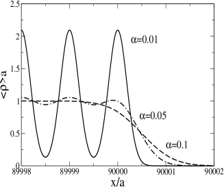
Figure 3: Average ground state density of a chain with $90000$ atoms near the right end of the chain for different values of $\alpha$. For $\alpha=0.01$ (full curve) the lattice structure is still pronounced. It is much weaker for $\alpha=0.05$ (dashed-dotted curve) and no longer visible for $\alpha=0.1$ (dotted curve).

Now, we address the general finite temperature quantum statistical mechanics result Eq. (50) for the mean square fluctuations. Even at small temperatures $\eta=k_{B}T/\hbar\omega_{s}\ll 1$, the very low energy modes $\hbar\omega_{j}\approx\hbar ck_{j}\ll k_{B}T$ are highly excited, i.e. $n_{B}(\omega_{j})\approx k_{B}T/\hbar\omega_{j}$. If $n$ is large enough, there is therefore a contribution to the $k$-sum dominated by the $1/k_{j}^{2}$ behavior leading to a linear in $n$ contribution. For small $n$ and $\eta=k_{B}T/\hbar\omega_{s}\ll 1$ the $T=0$ behaviour dominates. The resulting crossover from logarithmic to linear increase with $n$ is shown in Fig. 4 for different values of the (small) temperature.

In the following subsection the fluctuations $\langle(\hat{u}_{l+n}-\hat{u}_{l})^{2}\rangle$ play an important role which are obtained by replacing $(\xi_{n}^{(j)})^{2}$ in Eq. (50) by $(\xi_{n+l}^{(j)}-\xi_{l}^{(j)})^{2}$. For $l+n$ and $l$ sufficiently far from the boundaries and $|n|$ sufficiently large $\langle(\hat{u}_{l+n}-\hat{u}_{l})^{2}\rangle\approx\langle\hat{u}_{n}^{2}\rangle\$ holds.

Figure 4: Finite temperature quantum statistical mechancis result for $\langle\hat{u}_{n}^{2}\rangle$ scaled by $\alpha a^{2}$ for $N=1000$ and different small temperatures: $\eta=0.001$ (dotted line), $\eta=0.0025$ (full line) $\eta=0.01$ (dashed line) and $\eta=0.05$ (dashed-dotted line).

III.3 Experimental implications

The properties of the chain, like the loss of long range order, can be studied experimentally by the scattering of a test particle with incoming momentum $\vec{p}_{i}$ to a final momentum $\vec{p}_{f}$. If the interaction of the test particle at position $\vec{X}$ with the chain atoms is described by a potential $V_{s}=\sum_{i=1}^{N}v(\vec{X}-\vec{x}_{n})$, the scattering cross section in Born approximation involves matrix elements of the operators $\exp{(i\vec{q}\cdot\hat{\vec{x}_{n}})}$, where $\hbar\vec{q}=\vec{p}_{f}-\vec{p}_{i}$ is the scattering wave vector AM . For the chain of atoms aligned on the $x$-axis only $q\equiv q_{x}$ appears in the static and dynamic structure factor. The static structure factor $S(q)$ which enters the cross section for X-ray scattering in Born approximation reads AM

$$S_{N}(q)\equiv\frac{1}{N}\langle\hat{\rho}_{q}\hat{\rho}_{-q}\rangle=\frac{1}{N}\sum_{n,l=1}^{N}e^{-iqa(n-l)}\langle e^{-iq(\hat{u}_{n}-\hat{u}_{l})}\rangle.$$ (60)

In order to evaluate $S(q)$ we use $\langle e^{\hat{A}}\rangle=e^{\langle\hat{A}^{2}\rangle/2}$ and obtain

$$S_{N}(q)=\frac{1}{N}\sum_{n,l=1}^{N}e^{-iqa(n-l)}e^{-q^{2}\langle(\hat{u}_{n}-\hat{u}_{l})^{2}\rangle/2}.$$ (61)

In a classical description the factor containing the displacements is absent at $T=0$ and the structure factor follows performing the geometric series as

$$S_{N}^{(0)}(q)=\frac{1}{N}\left[\frac{\sin{(qaN/2)}}{\sin{(qa/2)}}\right]^{2}$$ (62)

For finite $N$ this leads to Bragg peaks at $q=2\pi\nu/a\equiv Q_{\nu}$ with peak height $N$ and width $1/N$. Except for $\nu=0$ (forward scattering) the Bragg peaks of the ideal static lattice are weakened by the second exponential factor on the rhs of Eq. (61) which involves expectation values discussed in the previous subsection. In the following we present numerical results for long but finite chains as well as analytical results in various limiting cases.

The double sum in Eq. (61) can be numerically evaluated for finite chains. Results are shown in Fig. (5) for a chain with $N=1000$ atoms and $\alpha=0.02$. As $S_{N}(0)=N$ the region near $q=0$ is suppressed. The dashed-dotted curve for $\eta_{cl}=0.03$ which is closest to the classical limit looks similar to the static structure factor of a simple liquid in three dimensions with a (broadened) peak resulting from the typical nearest neighbour distances Chandler .

This behaviour can be understood analytically in the strict classical limit $\alpha=0$. Then the result for the relative fluctuation of the chain simplifies to $\langle(\hat{u}_{n}-\hat{u}_{l})^{2}\rangle=\eta_{cl}a^{2}|n-l|$ for all distances.

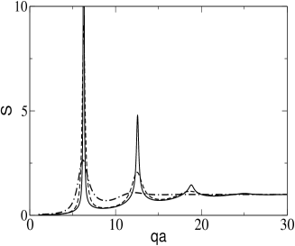
Figure 5: Static structure factor for a chain with $N=1000$ atoms and $\alpha=\hbar/(mca)=0.02$ for various values of $\eta_{cl}=k_{B}T/(mc^{2})$. The dashed-dotted curve for $\eta_{cl}=0.03$ shows “liquid-like” behaviour where only a Bragg peak at $q=2\pi/a$ is clearly seen. For $\eta_{cl}=0.01$ (dashed curve) also the peak at $q=4\pi/a$ is visible. For the full curve with $\eta_{cl}=0.001$ the quantum effects discussed in the text are important.The forward scattering peak with $S_{N}(0)=N$ is suppressed.

Therefore the double sum in Eq. (61) can be reduced to a single sum using

$$\frac{1}{N}\sum_{l,n=1}^{N}G(n-l)=G(0)+2\sum_{m=1}^{N-1}\left(1-\frac{m}{N}\right)G_{e}(m),$$ (63)

where $G_{e}$ is the even part of the arbitrary function $G$. In the limit $N\to\infty$ the geometric series which is convergent for $q\neq 0$ leads to Emery

$$S_{\infty}^{(cl)}(q)=\frac{\sinh(\eta_{cl}q^{2}a^{2}/2)}{\cosh(\eta_{cl}q^{2}a^{2}/2)-\cos(qa)}~{}.$$ (64)

As the limits $N\to\infty$ and $q\to 0$ do not commute the forward scattering peak is lost. Near the Bragg positions $Q_{\nu}$ with nonzero $\nu$, i.e. $qa=2\pi\nu+\tilde{q}a$ and $\tilde{q}a\ll 1$ one can expand the cosine function in the denominator. For $\eta_{cl}Q_{\nu}^{2}a^{2}\ll 1$ this leads to well defined Lorentzian Bragg peaks of width $2\pi^{2}\nu^{2}\eta_{cl}/a$. For finite temperatures this can happen only for small values of $|\nu|$ and already for $\eta_{cl}=0.01$ the structure factor looks liquid-like.

As the quantum parameter $\alpha$ is not strictly zero for the results in Fig. 5 but chosen as $\alpha=0.02$ the dashed-dotted curve has an additional broadening due to quantum fluctuations. Reducing the temperature they become more important for $\eta_{cl}=0.01$ (dotted curve) and prominent for $\eta_{cl}=0.001$ (full curve). The peak height at $q=Q_{1}$ for this parameter value is $\approx 36.7$.

For small values of $\alpha$ and $T=0$ one has to work with very long chains to see the divergent power law shape of the low index Bragg peaks which emerges in the infinite chain limit. In order to determine the divergent contribution one can approximate the sum by using the long distance logarithmic dependence of $\langle(\hat{u}_{l+n}-\hat{u}_{l})^{2}\rangle$ for all distances $|n|>n_{0}$, where $n_{0}>1$ can be chosen arbitrarily. Using $e^{-\beta\log{n}}=1/n^{\beta}$ one obtains for the possibly divergent contribution (indicated by “$div$” on top of the equal sign)

$$S_{\infty}(q)\stackrel{{\scriptstyle div}}{{=}}2\lim_{N\to\infty}\sum_{n=n_{0}}^{N}\cos(qan)\left(1-\frac{n}{N}\right)\frac{1}{n^{\beta(q)}}~{},$$ (65)

where

$$\beta(q)\equiv\frac{\alpha}{2\pi}(aq)^{2}.$$ (66)

At the Bragg positions $q=Q_{\nu}$, the sum is finite for $\beta(Q_{\nu})=2\pi\alpha\nu^{2}>1$ and diverges for $2\pi\alpha\nu^{2}\leq 1$. As we assume $\alpha\ll 1$ the sum $S_{\infty}(Q_{\nu})$ diverges for a few low index Bragg peaks, but is finite for sufficiently large $|\nu|$. In order to determine the divergence with $N$ at the low index Bragg positions $Q_{\nu}$ with $\nu\neq 0$ the sum in Eq.(65) can be converted to an integral which can easily be performed as the cosine factor equals $1$. Both terms have the same divergent behaviour, only the prefactors differ. For $0<\beta(Q_{\nu})<1$ one obtains

$$T=0:~{}~{}~{}~{}~{}~{}~{}~{}~{}~{}S_{N}(Q_{\nu})\sim N^{1-2\pi\alpha\nu^{2}}~{}.$$ (67)

For $\beta(Q_{\nu})<1$ the divergent peak shape for $q=Q_{\nu}+\tilde{q}$ in the small $\tilde{q}a$ limit is also determined by the large $n$ behaviour of the sum. In order to read-off the divergent contribution to $S_{\infty}(Q_{\nu}+\tilde{q})$ for $\nu\neq 0$ one can again replace the sum by an integral. This yields after the substitution $u=|\tilde{q}|an$

$$S_{\infty}(Q_{\nu}+\tilde{q})\stackrel{{\scriptstyle div}}{{=}}2(|\tilde{q}|a)^{\beta(q)-1}\int_{\tilde{q}an_{0}}^{\infty}\frac{\cos u}{u^{\beta(q)}}du~{}.$$ (68)

Because of the cosine factor the upper limit of the integral poses no problem as $\beta(q)>0$. For $\beta(q)<1$ the integral is also non-divergent at the lower limit for $\tilde{q}\to 0$. In this limit $\beta(q)$ in the prefactor can be replaced by $\beta(Q_{\nu})$. This leads to the power law divergence of the static structure factor near the Bragg peaks with $\beta(Q_{\nu})<1$

$$S_{\infty}(Q_{\nu}+\tilde{q})\sim(|\tilde{q}|a)^{\beta(Q_{\nu})-1}=(|\tilde{q}|a)^{2\pi\alpha\nu^{2}-1}.$$ (69)

As we have only focussed on the divergent part of $S_{\infty}$ in Eq. (68) the power law divergence of Eq. (69) does not imply that $S_{\infty}$ vanishes in a power law fashion in $|\tilde{q}|$ at the Bragg positions with $\beta(Q_{\nu})>1$.

As a second experimental probe we shortly discuss Mössbauer spectroscopy which is a local probe Lipkin . We assume that the nuclei of the atoms in the chain have an excited state which can decay to the ground state by emitting a gamma ray. In this process the momentum $-\hbar\vec{q}$ is transferred to the atom which emits the gamma quantum with wavevector $\vec{q}$. The energy of the emitted gamma quantum depends on the recoil energy transmitted to the crystal. There is a finite probability that the emitted gamma ray is absorbed by another nucleus of the same type. This recoilless emission is called “Mössbauer effect”. If the harmonic crystal is in an eigenstate $|E_{n}\rangle$ initially (with $n$ a multi-index), the state after the gamma emission from the atom with the position $\vec{x}_{l}$ is given by $\exp{(-i\vec{q}\cdot\hat{\vec{x}_{l}})}|E_{n}\rangle$. The energy spectrum of the emitted gamma ray relative to its energy for a fixed nucleus is obtained by expanding this state into eigenstates of the harmonic crystal and averaging over the canonical probability for the initial state $|E_{n}\rangle$,

$$P_{l}(\epsilon)=\sum_{n,m}\frac{e^{-\beta E_{n}}}{Z}|\langle E_{m}|e^{-i\vec{q}\cdot\hat{\vec{x}_{l}}}|E_{n}\rangle|^{2}\delta(\epsilon+(E_{m}-E_{n})).$$ (70)

Using the Fourier representation of the delta function it is straightforward to calculate this function for the harmonic chain with the help of the operator identities presented in the previous sections.

Here we only address the question how at $T=0$ the quantum fluctuations suppress recoilless emission. For the one-dimensional chain only $q\equiv q_{x}$ enters and the probability not to excite phonons is given by

$$p_{l}^{(0)}=|\langle E_{0}|e^{-iq\hat{u}_{l}}|E_{0}\rangle|^{2}=e^{-q^{2}\langle\hat{u}_{l}^{2}\rangle_{0}}~{}.$$ (71)

Using the infinite chain result Eq. (III.2) one finds that the probability for recoilless emission decreases as a power law with the distance from the fixed left end of the chain.

$$p_{l}^{(0)}\sim l^{-\beta(q)}~{},$$ (72)

with $\beta(q)$ defined in Eq. (66).

As a third experimental probe neutron scattering could be discussed with the help of the dynamic structure factor.AM ; Mikeska .

IV Outlook

We have shown how classical thermal fluctuations and quantum fluctuations at $T=0$ destroy the long range order in an infinite chain in a very different way. Both results are caused by the low energy phonon modes with frequency $\omega(k)\approx ck$. In the classical high temperature limit the linear divergence of $\langle\hat{u}_{n}^{2}\rangle$ with $n$ is due to the $1/k^{2}$ divergence of the integrand in Eq. (III.2). The factor $\sin^{2}(kn)$ leads to a small $k$ cutoff $k_{\rm min}\sim 1/n$ for the $k$-integration. At $T=0$ the quantum fluctuations follow from the $1/k$ divergence of the integrand in Eq. (III.2), the cutoff being the same. This leads to the slow logarithmic divergence of $\langle\hat{u}_{n}^{2}\rangle$ with $n$, i.e. crystalline long range order is destroyed even at zero temperature.

The findings for the infinite one-dimensional chain can be generalized to higher dimensional harmonic lattices by putting the atoms e.g. on a square lattice or a simple cubic lattice. The low frequency modes are again sound wavesAM with $\omega(\vec{k})\approx c|\vec{k}|\equiv ck$. The mean square deviations can be calculated as for the one-dimensional chain in Eq. (50). The possibly diverging part again comes from the small $k$ contribution with the $dk$ in the infinite chain limit replaced by the $d$-dimensional integration measure proportional to $k^{d-1}dk$. Multiplying with $1/k^{2}$ for the thermal fluctuations yields for the possibly diverging contribution $\sim\int_{k_{min}}k^{d-3}dk$ and multiplying with $1/k$ for the quantum fluctuations at $T=0$ to $\sim\int_{k_{min}}k^{d-2}dk$. In the three-dimensional case even the thermal fluctuations lead to a finite result in the limit $k_{min}\to 0$ i.e. long range crystalline order exists as noted by Peierls Peierls . For $d=2$ the quantum fluctuations are finite in this limit but a logarithmic divergence is produced by the thermal fluctuations. The divergence due to quantum fluctuations in $d$ dimensions is of the same type as from the (classical) thermal fluctuations in $d+1$ dimensions, where in our example $d=1$.

Extensions of this finding for harmonic lattices can be found in the literature on quantum phase transitions Sachdev . This are phase transitions not as a function of tempertature but as a function of a system parameter at zero temperature. The harmonic chain with the additional harmonic potentials of strenght $\lambda_{loc}$ centered at the lattice positions discussed following Eq. (45) has a quantum phase transition at $\lambda_{loc}=0$. For all positive values of $\lambda_{loc}$ the fluctuations around the lattice positions stay finite and well defined Bragg peaks exist. For $\lambda_{loc}=0$ the zero temperature quantum fluctuctions diverge logarithmically and no crystalline order exists. This “one-sided” quantum phase transition is of a very special type as only values $\lambda_{loc}\geq 0$ correspond to stable systems.

V Acknowledgements

The author would like to thank G. Hegerfeldt, V. Meden, H.J. Mikeska and D. Vollhardt for a critical reading of the manuscript.

References

- (1) K. Huang, Introduction to Statistical Physics (Taylor and Francis, London, 2001)
- (2) G. Baym, Lectures on Quantum Mechanics (Benjamin, Reading, MA, 1969)
- (3) E. Merzbacher, Quantum Mechanics 3rd edition (John Wiley and Sons, New York, 2000)
- (4) A. Messiah Quantum Mechanics (North-Holland, Amsterdam, 1967), Vol. 1.
- (5) R.E. Peierls, “Bemerkungen über Umwandlunstemperaturen”, Helv. Phys. Acta 7, Supplement II, 81-83 (1934)
- (6) N.W. Ashcroft and N.D. Mermin, Solid State Physics (Holt, Rinehart and Winston, New York, 1976)
- (7) B. Jancovici, “Infinite susceptibility without long-range order: the two-dimensional harmonic ’solid”’, Phys. Rev. Letters, 19, 20-22 (1967)
- (8) H.J. Mikeska and H. Schmidt, “Phase transitions without long-range order in two dimensions”, J. Low Temp. Phys. 2, 371-381 (1970)
- (9) A.L. Fetter, J.D. Walecka, Quantum Theory of Many-Particle Systems (Mc-Graw Hill, New York, 1971)
- (10) D. Mermin, “A short simple derivation of expressions of the Debye-Waller form”, J. Math. Phys. 7, 1038-1039 (1966)
- (11) S. Tomonaga, “Remark on Bloch’s method of sound waves applied to many fermion problems”, Progr. Theor. Phys. 5, 544-569 (1950)
- (12) J.M. Luttinger, “An exactly soluble model of many fermion systems”, J. Math. Phys. 4, 1154-1162 (1963)
- (13) F.D.M. Haldane, “ ’Luttinger liquid theory’ of one dimensional quantum fluids: I. Properties of the Luttinger model and their extension to the general 1D interacting spinless Fermi gas”, J. Phys. C 14, 2585-2919 (1981)
- (14) K. Schönhammer and V. Meden, “ Fermion-boson transmutation and comparison of statistical ensembles in one dimension”, Am. J. Physics 64, 1168-1176 (1996)
- (15) D. Chandler, Introduction to Modern Statistical Mechanics (Oxford University Press, 1987)
- (16) V.J. Emery and J.D. Axe, “One-dimensional fluctuations at the chain ordering transformation in ”, Phys. Rev. Lett. 40, 1507 (1978)
- (17) H.I. Lipkin, Quantum Mechanics, New Approaches to Selected Topics (North-Holland, Amsterdam, 1973)
- (18) H.J. Mikeska, “Phonon peaks in the dynamic structure function of lattices without long range order”, Solid State Commun. 13, 73-76 (1973)
- (19) S. Sachdev, Quantum Phase Transitions (Cambridge University Press, 2011 (second edition))