Instability Margin Analysis for Parametrized LTI Systems with Application to Repressilator

Abstract

This paper is concerned with a robust instability analysis for the single-input-single-output unstable linear time-invariant (LTI) system under dynamic perturbations. The nominal system itself is possibly perturbed by the static gain of the uncertainty, which would be the case when a nonlinear uncertain system is linearized around an equilibrium point. We define the robust instability radius as the smallest $H_{\infty}$ norm of the stable linear perturbation that stabilizes the nominal system. There are two main theoretical results: one is on a partial characterization of unperturbed nominal systems for which the robust instability radius can be calculated exactly, and the other is a numerically tractable procedure for calculating the exact robust instability radius for nominal systems parametrized by a perturbation parameter. The results are applied to the repressilator in synthetic biology, where hyperbolic instability of a unique equilibrium guarantees the persistence of oscillation phenomena in the global sense, and the effectiveness of our linear robust instability analysis is confirmed by numerical simulations.

Keywords: analysis of systems with uncertainties, robust instability, instability margin, periodic oscillation, repressilator

1 Introduction

Feedback control to maintain non-equilibrium state such as oscillation has been recognized as an important design problem for engineering applications including robotic locomotion (Grizzle et al., 2001; Wu & Iwasaki, 2021). Such non-equilibrium state may be robustly maintained if every equilibrium point is hyperbolically unstable (Pogromsky et al., 1999). This fact motivates robust instability analysis of an equilibrium point subject to perturbations. For linear systems, analysis of robust instability is equivalent to finding the minimum norm stable controller that stabilizes a given unstable plant, which is known to be extremely difficult due to the requirements of the strong stabilization (Youla et al., 1974) and the norm constraint on the controller. The analysis is further complicated by the fact that equilibrium points may change due to perturbations in nonlinear dynamical systems. When the equilibrium is perturbed, the linearized dynamics would be altered, and hence an analysis of a fixed linearized system no longer characterizes the robustness property of the equilibrium point. This issue has been pointed out in the context of a robust stability analysis for Lur’e type nonlinear systems (Wada et al., 1998, 2000), as well as in a robust bifurcation analysis (Inoue et al., 2015). Thus, we need to develop a theory to address this issue properly with a general framework to lay a foundation for the linear robust instability theory.

In this paper, we formally define the robust instability radius (RIR) for single-input-single-output (SISO) unstable linear time invariant (LTI) systems subject to dynamic perturbations (Inoue et al., 2013a) in a manner analogous to the classical robust stability radius (Hinrichsen & Pritchard, 1986). A key technical result shows that the RIR analysis reduces to a marginal stabilization problem, leading to two conditions under which the exact RIR is given as the inverse of the static or peak gain of the system. We will then extend our analysis to rigorously take account of the possible change of the nominal linear dynamics caused by the perturbation. The main theoretical result of this part leads to a computationally tractable procedure to find the exact RIR for a class of parametrized LTI systems. Finally, the effectiveness of the theoretical results will be demonstrated through numerical simulations by an application to the repressilator (Elowitz & Leibler, 2000).

Our approach builds on the preliminary result (Hara et al., 2020), which formalized the robust instability analysis problem for a fixed LTI system by introducing a notion of the RIR. The contributions of the present paper beyond (Hara et al., 2020) include theoretical justification of the marginal stabilization approach, a characterization of third order systems for which the RIR can be found exactly, and an extension to the parametrized LTI systems to account for the change of the nominal dynamics due to the perturbation.

The remainder of this paper is organized as follows. Sections 2 and 3 are devoted to the analyses of the RIR for fixed and parametrized LTI systems, respectively. The effectiveness of the theoretical results is confirmed by an application to the repressilator model in Section 4. Section 5 summarizes the contributions of this paper and addresses some future research directions.

We use the following notation. The set of real numbers is denoted by $\mathbb{R}$. $\Re(s)$ denotes the real part of a complex number $s$. The set of real rational functions bounded on $j\mathbb{R}$ is denoted by $\mathbb{R}\mathbb{L}_{\infty}$, and its stable subset by $\mathbb{R}\mathbb{H}_{\infty}$. The norms in these linear spaces are denoted by $\|\cdot\|_{L_{\infty}}$ and $\|\cdot\|_{H_{\infty}}$, respectively. The open left and right half complex planes are abbreviated as OLHP and ORHP, respectively.

2 Robust Instability Radius for LTI Systems

This section is devoted to the analysis of the robust instability radius (RIR) for a given unstable transfer function $g(s)\in\mathbb{R}\mathbb{L}_{\infty}$. We will provide two classes of $g(s)$ for which the RIR can be characterized exactly.

2.1 Definition and Preliminary Results on RIR

Our target system is an unstable system represented by the transfer function $g(s)$ which has no poles on the imaginary axis, i.e., $g(s)\in\mathbb{R}\mathbb{L}_{\infty}$. Given such $g(s)$, we introduce a set denoted by $\mathbb{S}(g)$ as follows: It is the set of $\mathbb{R}\mathbb{H}_{\infty}$ functions $\delta(s)$ that internally stabilizes $g(s)$ with positive feedback, that is, $\mathbb{S}(g)$ is defined as

$$\mathbb{S}(g) := \Big{\{}~{}\delta(s)\in\mathbb{R}\mathbb{H}_{\infty}:~{}$$ (3)

$$\begin{array}[]{l}\delta(s)g(s)=1~{}\Rightarrow~{}\Re(s)<0\vspace*{-1mm}\\ \delta(s)=0,\Re(s)>0~{}\Rightarrow~{}|g(s)|<\infty\end{array}\Big{\}}.\vspace*{-2mm}$$

The first condition of $\mathbb{S}(g)$ means that the characteristic roots of the positive feedback connection of $\delta(s)$ and $g(s)$ are in the OLHP, and the second one implies that $\delta(s)$ and $g(s)$ have no unstable pole/zero cancellation for the internal stability. In this sense, ”stabilization” in this paper means ”internal stabilization.”

Let us first define the robust instability radius (RIR) for a given $g(s)\in\mathbb{R}\mathbb{L}_{\infty}$, which will be useful for later developments. The RIR for $g(s)$, denoted by $\rho_{*}$, is defined to be the magnitude of the smallest perturbation that stabilizes $g(s)$, i.e.,

$$\vspace*{-2mm}\rho_{*}:=\inf_{\delta\in\mathbb{S}(g)}~{}\|\delta\|_{H_{\infty}}.\vspace*{-2mm}$$ (4)

It is clear from the condition for the strong stabilizability in (Youla et al., 1974) that $\mathbb{S}(g)$ is nonempty and hence $\rho_{*}$ for $g(s)$ is finite if and only if the Parity Interlacing Property (PIP) is satisfied, i.e., the number of unstable real poles of $g(s)$ between any pair of real zeros in the closed right half complex plane (including zero at $\infty$) is even.

Some lower bounds of $\rho_{*}$ are known from the literature as follows.

Lemma 1

(Inoue et al., 2013a, b; Hara et al., 2020)   Let $g(s)\in\mathbb{R}\mathbb{L}_{\infty}$ be given. Suppose $g(s)$ is strictly proper and unstable. Then

$$\vspace*{-3mm}\rho_{*}\geq~{}{\rho}_{p}:=1/\|g\|_{L_{\infty}},\hskip 8.53581pt\|g\|_{L_{\infty}}:=\sup_{\omega\in\mathbb{R}}|g(j\omega)|.\vspace*{-3mm}$$ (5)

Moreover, if $g(s)$ has an odd number of unstable poles (including multiplicities) then we have

$$\vspace*{-3mm}\rho_{*}\geq{\rho}_{o}:=1/|g(0)|.\vspace*{-3mm}$$ (6)

The lower bounds given above can readily be calculated, immediately giving an estimate for the RIR. It will turn out later that each of these bounds is tight for a certain case, providing the exact value of the RIR $\rho_{*}$. To that end, we will develop an approach for characterizing an upper bound in a tractable manner, and provide conditions under which the upper bound coincides with one of the lower bounds ${\rho}_{o}$ and ${\rho}_{p}$. These are addressed in the following subsections.

2.2 Upper bound via marginal stabilization

An upper bound is obtained as $\|\delta\|_{H_{\infty}}$ if a stable stabilizing perturbation $\delta(s)$ is found. Since the closed-loop poles for such perturbation are in the open left half plane, a scaled perturbation $(1-\varepsilon)\delta(s)$ is also stabilizing for sufficiently small $\varepsilon>0$, and has smaller norm $(1-\varepsilon)\|\delta\|_{H_{\infty}}$, yielding a better (smaller) upper bound. This observation leads to the fact that the best (least norm) upper bound is necessarily obtained from a perturbation that marginally stabilizes the closed-loop system. Hence, we may focus on the search for a marginally stabilizing, stable perturbation $\delta_{o}(s)$. However, such $\delta_{o}(s)$ does not necessarily give an upper bound since a slight perturbation of $\delta_{o}(s)$ may not be able to (strictly) stabilize the closed-loop system in general. The following result shows that an upper bound can always be obtained if marginal stability is achieved with a single mode on the imaginary axis.

Proposition 1

Consider real-rational transfer functions $g(s)$ and $\delta_{o}(s)$ having no unstable pole/zero cancellation between them, where the former is strictly proper and the latter is proper and stable (possibly a real constant). Suppose $\delta_{o}(s)$ marginally stabilizes $g(s)$ with the closed-loop characteristic roots of $\delta_{o}(s)g(s)=1$ all in the OLHP except for either a pole at the origin or a pair of complex conjugate poles on the imaginary axis. Then, for almost any proper stable transfer function $\delta_{1}(s)$, there exists $\varepsilon\in\mathbb{R}$ of arbitrarily small magnitude $|\varepsilon|$ such that the positive feedback with $\delta_{\varepsilon}(s):=\delta_{o}(s)+\varepsilon\delta_{1}(s)$ internally stabilizes $g(s)$.

See Appendix A for a proof of the proposition.

When a stable perturbation $\delta_{o}(s)$ achieves marginal stability with multiple modes on the imaginary axis (which is a rather rare occasion), every slight modification of $\delta_{o}(s)$ may move at least one purely imaginary pole into the right half plane. In this case, $\|\delta_{o}\|_{H_{\infty}}$ is not an upper bound on the RIR. However, Proposition 1 shows that, when there is a single mode on the imaginary axis (which is generically expected), almost every perturbation of $\delta_{o}(s)$ moves the imaginary pole(s) in a direction transverse to the imaginary axis, and hence it is always possible to strictly stabilize the closed-loop system. Therefore, an upper bound can be obtained by searching for such $\delta_{o}(s)$.

Given the extreme difficulty of strong stabilization with the minimum norm controller, Proposition 1 is significant because (a) the search for such marginally stabilizing $\delta_{o}(s)$ can be performed systematically by restricting our attention to some specific class of transfer functions, and (b) this approach is suitable for the search for the minimum norm, marginally stabilizing perturbation $\delta_{o}(s)$. These claims are explained in the next section.

2.3 Search for marginally stabilizing perturbation

First note that marginal stability requires that $\delta_{o}(s)$ be chosen to satisfy

$$\vspace*{-3mm}\delta_{o}(j\omega_{c})=\delta_{c}:=1/g(j\omega_{c}),\vspace*{-3mm}$$ (7)

at a critical frequency $\omega_{c}\geq 0$, so that $s=j\omega_{c}$ is a closed-loop pole. If we parametrize a class of perturbations, then $\delta_{o}(s)$ satisfying (7) may be determined for each $\omega_{c}\in\mathbb{R}$, and an upper bound $\|\delta_{o}\|_{H_{\infty}}$ on the RIR is obtained when the resulting closed-loop poles (i.e. roots of $\delta_{o}(s)g(s)=1$) are all in the OLHP except for $s=\pm j\omega_{c}$ (let us call this property $\omega_{c}$-stability).

A reasonable candidate for the class of $\delta_{o}(s)$ is the set of all-pass transfer functions (Hara et al., 2020). An advantage of using all-pass functions is that the least upper bound on the RIR is obtained for a given $\omega_{c}$ since the gap in $\|\delta_{o}\|_{H_{\infty}}\geq|\delta_{o}(j\omega_{c})|$ is eliminated regardless of the value of $\omega_{c}$. The simplest choice is the first (or zeroth) order all-pass function expressed as

$$\vspace*{-3mm}\delta_{o}(s)=b\cdot\frac{s-a}{s+a},\hskip 8.53581pt(a\geq 0).\vspace*{-3mm}$$ (8)

There are two requirements for choosing the parameters $(a,b)$ in $\delta_{o}(s)$. One is (7) and the other is $a\geq 0$ to assure stability of $\delta_{o}(s)$. A simple calculation leads to $|b|=|\delta_{c}|$ and $\angle(j\omega_{c}-a)-\angle(j\omega_{c}+a)+\angle(b)=\angle(\delta_{c})$, which gives the proper choice of $(a,b)$ as follows:

$$\vspace*{-2mm}\begin{array}[]{lll}a=\omega_{c}\tan\varphi,&b=|\delta_{c}|,&(0\leq\varphi<\pi/2),\\ a=\omega_{c}\tan(\varphi+\pi/2),&b=-|\delta_{c}|,&(-\pi/2\leq\varphi<0),\end{array}\vspace*{-2mm}$$ (9)

where $\varphi:=\angle\delta_{c}/2$. Thus, for a given $\omega_{c}\in\mathbb{R}$, the stable first order all-pass function (8) is uniquely determined. The gain $\|\delta_{o}\|_{H_{\infty}}$ is then an upper bound on the RIR if the $\omega_{c}$-stability is achieved by $\delta_{o}(s)$. Sweeping over $\omega_{c}\in\mathbb{R}$, the least upper bound within this framework can be calculated.

2.4 Simple classes of $g(s)$ for which the exact RIR can be analytically characterized

In view of Lemma 1, important cases occur when the $\omega_{c}$-stability is achieved at $\omega_{c}=0$ or $\omega_{p}$, where $\omega_{p}$ is the peak frequency at which $|g(j\omega_{p})|=\|g\|_{L_{\infty}}$ holds. In these cases, the exact values of the RIR is given by $\rho_{*}=1/|g(j\omega_{c})|$ because the upper and lower bounds coincide. In particular, we have the following:

• $\rho_{*}=\rho_{o}$ if $g(s)$ satisfies Condition 1: $g(s)\in\mathbb{R}\mathbb{L}_{\infty}$ has an odd number of poles (including multiplicities) in the ORHP, and the constant perturbation $\delta_{o}(s)=1/g(j\omega_{c})$ achieves the $\omega_{c}$-stability with $\omega_{c}=0$.

• $\rho_{*}=\rho_{p}$ if $g(s)$ satisfies Condition 2: $g(s)\in\mathbb{R}\mathbb{L}_{\infty}$ is unstable, and $\delta_{o}(s)$ in (8) with (9) achieves $\omega_{c}$-stability at $\omega_{c}=\omega_{p}$.

While it is easy to construct $\delta_{o}(s)$ numerically for a given $g(s)$ and check $\omega_{c}$-stability of the closed-loop system, it remains open to fully characterize the class of $g(s)$ which can be $\omega_{c}$-stabilized by a first-order all-pass function. Here we present a subclass of third order systems for which the above idea works. This class covers the simplest model of the repressilator in synthetic biology as seen in Section 4.

Proposition 2

Consider the third order transfer function represented by

$$g(s)=\frac{\zeta s-k}{s^{3}+ps^{2}+qs+\ell},\hskip 8.53581ptk\neq 0$$ (10)

(i) $g(s)$ satisfies Condition 1 if and only if

$$p>0,\hskip 8.53581pt\ell<0,\hskip 8.53581ptq+\zeta\ell/k>0,$$ (11)

which implies $\rho_{*}=\rho_{o}:=1/|g(0)|$.
(ii) $g(s)$ satisfies Condition 2 if

$$p>0,\hskip 8.53581pt\ell>pq,\hskip 8.53581ptq^{2}<2p\ell,$$ (12)

which implies $\rho_{*}=\rho_{p}:=1/\|g\|_{L_{\infty}}$.

See Appendix B for a proof of the proposition.

There are three remarks on the class of $g(s)$ of the form (10) satisfying (12): (i) The requirement of $\ell>pq$ is necessary and sufficient for $g(s)$ to have two unstable poles, provided $p>0$ and $\ell>0$, which are guaranteed by the first and third inequalities in (12). (ii) The requirement of $q^{2}<2p\ell$ is a sufficient condition for the infinity norm of $g(s)$ to be attained at a non-zero frequency. (iii) A class of third order systems represented by $g(s)=k/((s+\alpha)(s^{2}-\beta s+\gamma^{2}))$ with $0<\beta<\gamma<\alpha$ satisfies (12) and hence Condition 2, which was numerically verified earlier in (Hara et al., 2020).

3 RIR for Parametrized LTI Systems

Here we derive a general theoretical result to provide a computationally tractable method for characterizing the exact robust instability radius $\mu_{*}$ for a class of parameterized linear systems based on the instability radius analysis in the previous section.

3.1 Definition of RIR $\mu_{*}$

We consider a family of SISO transfer functions $g_{e}(s)$ parameterized by $e\in\mathbb{R}$, where we assume that $g_{e}(s)$ has at least one pole in the ORHP and no poles on the imaginary axis for all $e\in\,\mathbb{E}:=(e_{-},e_{+})$ which includes the origin, i.e., $e_{-}<0<e_{+}$. For each $e\in\mathbb{E}$, let $\Delta_{e}$ be the set of all perturbations $\delta(s)\in\mathbb{R}\mathbb{H}_{\infty}$ that stabilizes $g_{e}(s)$ and satisfies $\delta(0)=e$, i.e.,

$$\vspace*{-2mm}\Delta_{e}:=\{\delta(s)\in\mathbb{S}(g_{e}):~{}\delta(0)=e~{}\}.\vspace*{-2mm}$$ (13)

The objective is to calculate the robust instability radius $\mu_{*}$ for $g_{e}(s)$ defined by

$$\vspace*{-2mm}\mu_{*}:=\inf_{e\in\mathbb{E}}~{}\mu(e),\hskip 8.53581pt\mu(e):=\inf_{\delta(s)\in\Delta_{e}}\|\delta\|_{H_{\infty}},\vspace*{-2mm}$$ (14)

where we define $\mu(e):=\infty$ if $\Delta_{e}$ is empty and $\mu_{*}:=\infty$ if $\Delta_{e}$ is empty for all $e\in\mathbb{E}$. Note that $\rho_{*}$ is identical to $\mu(e)$ for $g_{e}(s)=g(s)$ except for the absence of the constraint on the static gain $\delta(0)=e$. The idea is that $g_{e}(s)$ is the system obtained by linearization of a nonlinear system around an equilibrium point, perturbed by the uncertainty $\delta(s)$ with static gain $e$.

As an example, let us consider a dynamically perturbed FitzHugh-Nagumo (FHN) neuron model presented in (Hara et al., 2020). We will show how to derive the corresponding $g_{e}(s)$ based on the uncertain FHN model

$$\begin{array}[]{l}c\dot{v}=\psi(v)-(1+\delta(s))w,\hskip 8.53581pt\psi(v):=v-v^{3}/3,\\ \tau\dot{w}=v+\alpha-\beta w,\end{array}$$

with positive constant parameters $c$, $\tau$, $\alpha$, and $\beta$, where the term $\tilde{w}:=(1+\delta(s))w$ represents the dynamically perturbed $w$ with uncertainty $\delta(s)$. Let $(\bar{v},\bar{w})$ be an equilibrium point, i.e.,

$$\psi(\bar{v})=(1+e)\bar{w},\hskip 8.53581pt\bar{v}=\beta\bar{w}-\alpha$$

hold, where $e:=\delta(0)$. It can be verified that the equilibrium is unique if $1+e>\beta$. Linearizing the system around $(\bar{v},\bar{w})$, the characteristic equation is given by $1=\delta(s)g_{e}(s)$ with

$$g_{e}(s):=1/\Big{(}c\tau s^{2}+(\beta c-\tau\gamma)s+1-\beta\gamma\Big{)},$$

where $\gamma:=\psi^{\prime}(\bar{v})=1-\bar{v}^{2}$. Note that $g_{e}(s)$ depends on $e$ through $\bar{v}$ since $\gamma$ is a function of $e$. The perturbation $\delta(s)$ stabilizes the equilibrium when it stabilizes $g_{e}(s)$ and has the consistent static gain $\delta(0)=e$.

The term RIR refers to both $\rho_{*}$ for a fixed LTI system and $\mu_{*}$ for parametrized LTI systems. While the mathematical definitions of $\rho_{*}$ and $\mu_{*}$ are different, both represent the smallest magnitude of perturbations that stabilize the underlying system (or equilibrium). In the special case where $g_{e}(s)$ is independent of $e$ (i.e. the equilibrium does not move by perturbation $\delta(s)$) and $\mathbb{E}=\mathbb{R}$, the RIR $\mu_{*}$ reduces to $\rho_{*}$. The final goal of this paper is provide a computable characterization for the robust instability radius $\mu_{*}$, which is the magnitude of the smallest perturbation $\delta(s)$ that stabilizes the equilibrium point of the nonlinear system.

3.2 Lemmas for Exact Analysis

This section presents three lemmas as preliminaries. All the proofs are given in Appendix C. Let us first examine the relationship between $\mu_{*}$ and $\rho_{*}$. The minimum value of $\mu(e)$ over $e\in\mathbb{E}$ is $\mu_{*}$ as seen in (14). A simple observation shows that $\mu(e)$ is closely related to the RIR for linear system $g_{e}(s)$, denoted by $\rho_{*}(e)$:

$$\rho_{*}(e):=\inf_{\delta\in\mathbb{S}(g_{e})}\|\delta\|_{H_{\infty}}.$$ (15)

In particular, $\rho_{*}(e)$ is a lower bound of $\mu(e)$.

Lemma 2

For each $e\in\mathbb{E}$, we have

$$\mu(e)\geq|e|,\hskip 8.53581pt\mu(e)\geq\rho_{*}(e).$$

Based on the results for the linear case, we expect that

$$\rho_{o}(e):=1/|g_{e}(0)|,\hskip 8.53581pt\rho_{p}(e):=1/\|g_{e}\|_{L_{\infty}},$$

may play an important role in characterizing $\mu_{*}$. In view of the results in the previous section, $\rho_{*}(e)$ is exactly characterized by $\rho_{o}(e)$ or $\rho_{p}(e)$, provided $g_{e}(s)$ satisfies Condition 1 or 2, respectively. Hence, the key for characterizing $\mu_{*}$ is to obtain the condition under which the lower bound $\rho_{*}(e)$ on $\mu(e)$ is tight, in which case, $\mu_{*}$ is given by the infimum of $\rho_{*}(e)$ over $e\in\mathbb{E}$. A technical difficulty is that when a stabilizing perturbation $\delta(s)$ is found for $g_{e}(s)$, it is likely that $\delta(0)=e$ is violated and hence such $\delta(s)$ cannot be used for the calculation of $\mu(e)$ in (14). The following result is useful for adjusting the static gain of $\delta(s)$ by a high pass filter while preserving the stabilizing property.

Lemma 3

Let $\gamma\in\mathbb{R}$ and scalar-valued, strictly proper, real-rational transfer function $\ell(s)$ be given. Suppose $\ell(s)$ has an even number of poles (including multiplicities) in the ORHP and no poles on the imaginary axis, all the roots of $1=\ell(s)$ are in the OLHP, and

$$|\gamma|<1,\hskip 8.53581pt\|\gamma\ell\|_{L_{\infty}}<1$$ (16)

hold. Then, for sufficiently small $\xi>0$, all the roots of

$$1=f(s)\ell(s),\hskip 8.53581ptf(s):=\frac{s+\xi\gamma}{s+\xi}$$ (17)

are in the OLHP.

Using Lemma 3 and the ideas from the RIR analysis, we can characterize $\mu(e)$ as follows.

Lemma 4

Fix $e\in\mathbb{R}$, let a strictly proper transfer function $g_{e}(s)$ be given, and consider $\Delta_{e}$ and $\mu(e)$ in (13) and (14), respectively. Suppose $|e|<\rho_{p}(e):=1/\|g_{e}\|_{L_{\infty}}$ holds and $g_{e}(s)$ satisfies the following conditions:

• $g_{e}(s)$ satisfies Condition 2.

• $g_{e}(s)$ has a nonzero even number of poles (including multiplicities) in the ORHP.

Then $\mu(e)=\rho_{p}(e)$ holds.

Condition (a) in Lemma 4 guarantees that $\rho_{p}(e)$ is the exact linear RIR for $g_{e}(s)$. However, the smallest perturbation $\delta(s)$ does not move the equilibrium to a point at which $g_{e}(s)$ is the corresponding linearization unless $\delta(0)=e$. Condition (b) allows for the use of Lemma 3 to adjust the static gain of the perturbation so that $\delta(s)$ with a high pass filter has the static gain $e$ and thus stabilization of $g_{e}(s)$ corresponds to stabilization of the original equilibrium point of the nonlinear system. It can be shown that conditions (a) and (b) hold for the class of third order systems with (12) in Proposition 2.

The static gain adjustment does not work for $g_{e}(s)$ satisfying Condition 1 since the number of poles in the ORHP is odd, in which case the perturbation with the high pass filter destabilizes $g_{e}(s)$. Hence, $\mu(e)=\rho_{o}(e)$ does not hold in general under Condition 1. The property $\mu(e)\geq\rho_{*}(e)=\rho_{o}(e)$ is still useful for obtaining lower and upper bounds on $\mu_{*}$, but does not seem to yield an exact characterization of $\mu_{*}$. Therefore, we will focus on the case where $g_{e}(s)$ satisfies the conditions in Lemma 4 in the next subsection.

3.3 Exact RIR Analysis

Lemma 4 characterizes $\mu(e)$ only when $e$ satisfies $|e|<\rho_{p}(e)$, and does not cover all possible values of $e\in\mathbb{E}$. However, it turns out that the minimum of $\mu(e)$ over $e\in\mathbb{E}$ occurs within the subset of $\mathbb{E}$ where $|e|<\rho_{p}(e)$ holds, and hence we have a computable description of $\mu_{*}$ as stated in the following theorem.

Theorem 1

Consider the parametrized LTI system $g_{e}(s)$ with $e\in\mathbb{E}\subset\mathbb{R}$, where $0\in\mathbb{E}$. Let $\mathbb{E}_{*}\subset\mathbb{E}$ be the largest interval such that $|e|<\rho_{p}(e)$ holds for $e\in\mathbb{E}_{*}$. Then

$$\mu_{*}=\inf_{e\in\mathbb{E}_{*}}\rho_{p}(e)$$ (18)

holds, provided $g_{e}(s)$ satisfies conditions (a) and (b) in Lemma 4 for all $e\in\mathbb{E}_{*}$.

Proof. Let $R_{\rm in}$ be the infimum of $\mu(e)$ over $e\in\mathbb{E}_{*}\subset\mathbb{E}$, and $R_{\rm out}$ be the infimum of $\mu(e)$ over $e\in\mathbb{E}\backslash\mathbb{E}_{*}$. Then $\mu_{*}=\min(R_{\rm in},R_{\rm out})$ by definition. We will show $R_{\rm in}\leq R_{\rm out}$ and hence $R_{\rm in}=\mu_{*}$. For contradiction, suppose $R_{\rm in}>R_{\rm out}$. Then there exists $e_{o}\in\mathbb{E}\backslash\mathbb{E}_{*}$ such that $\mu(e_{o})<R_{\rm in}$. Let us consider the case $e_{o}>0$. The case $e_{o}<0$ can be proven similarly. Since $\mathbb{E}$ and $\mathbb{E}_{*}$ are convex intervals containing $0$, there exists $e_{1}\in(0,e_{o})$ such that $(0,e_{1})\subset\mathbb{E}_{*}$ and $(e_{1},e_{o})\subset\mathbb{E}\backslash\mathbb{E}_{*}$. Then we have

$$R_{\rm in}\leq\rho_{p}(e_{1})=e_{1}<e_{o}\leq\mu(e_{o})<R_{\rm in}.$$ (19)

Here, $R_{\rm in}\leq\rho_{p}(e_{1})$ holds by definition of $R_{\rm in}$ and $(0,e_{1})\subset\mathbb{E}_{*}$, $\rho_{p}(e_{1})=e_{1}$ holds since $e_{1}$ is the upper boundary of $\mathbb{E}_{*}$ at which $\rho_{p}(e)<|e|$ is violated, $e_{1}<e_{o}$ and $\mu(e_{o})<R_{\rm in}$ hold by definition, and $e_{o}\leq\mu(e_{o})$ holds due to Lemma 2. However, (19) does not hold, and hence we conclude $R_{\rm in}\leq R_{\rm out}$ by contradiction.   

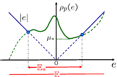
Figure 1: Computation for Exact RIR $\mu_{*}$

Theorem 1 provides a computable characterization of $\mu_{*}$ at an equilibrium point when conditions (a) and (b) are satisfied. Figure 1 illustrates the situation related to the proof of Theorem 1 by plotting $\rho_{p}(e)$ and $|e|$. This figure also helps to understand the following concrete procedure to calculate the exact RIR $\mu_{*}$:

• Step 1: Determine the subset $\mathbb{E}_{*}\subset\mathbb{E}$ defined in Theorem 1 by computing ${\rho}_{p}(e)$ for $e\in\mathbb{E}$.

• Step 2: Check conditions (a) and (b) in Lemma 4 for $e\in\mathbb{E}_{*}$. If they are satisfied, then compute the infimum of $\rho_{p}(e)$ over $\mathbb{E}_{*}$ which provides $\mu_{*}$. Otherwise, the infimum gives a lower bound of $\mu_{*}$.

4 Applications to Repressilator

4.1 Model of Repressilator

We consider a class of biomolecular systems in Fig. 2 motivated by applications in synthetic biology. This system is called repressilator (Elowitz & Leibler, 2000) and consists of three species of proteins P_i $(i=1,2,3)$, each of which is designed to repress the production of another protein species using the simple cyclic feedback. It is known that the repressilator in Fig. 2 has a single equilibrium point (Hori et al., 2011), and thus, destabilization of the equilibrium point leads to oscillatory dynamics of the concentrations of P_i, given that the trajectories are bounded. In the previous work (Niederholtmeyer et al., 2015), this mechanism was experimentally confirmed in vitro by tuning the parameters of synthetic biomolecular oscillators (see Potvin-Trottier et al. (2016) for discussion for in vivo).

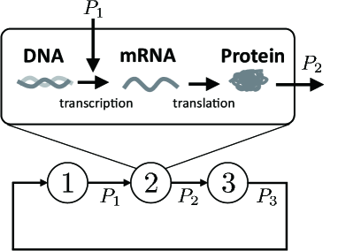
Figure 2: Model of the repressilator

The nominal dynamical model of the repressilator is given by the following ordinary differential equations:

$$\dot{x}_{i}(t)=-\alpha_{i}x_{i}(t)+\beta_{i}\psi_{i}(x_{i-1}(t)),\hskip 8.53581pti=1,2,3$$ (20)

where $x_{i}(t)$ is the concentration of protein P_i, $\alpha_{i}$ ($>0$) is the degradation rate of P_i, and $\beta_{i}$ ($>0$) is the gain of the interactions. The index $i$ is defined by modulo 3, implying that $x_{0}(t):=x_{3}(t)$. The function $\psi_{i}(\cdot)$ is a monotone decreasing static nonlinearity called Hill function (Alon, 2006) that represents the rate of protein production. Specifically,

$$\vspace*{-4mm}\psi_{i}(x)=\frac{K_{i}^{\nu_{i}}}{K_{i}^{\nu_{i}}+x^{\nu_{i}}},\hskip 8.53581pti=1,2,3\vspace*{-4mm}$$ (21)

with a Hill coefficient $\nu_{i}$ and a Michaelis-Menten constant $K_{i}$ ($>0$).

Our theoretical results are verified by the model of a typical experimental setting with the parameters chosen based on the experimental data in (Niederholtmeyer et al., 2015);

$$\vspace*{-6mm}\begin{array}[]{llll}\alpha_{1}=0.4621,&\beta_{1}=138.0,&K_{1}=5.0,&\nu_{1}=3\\ \alpha_{2}=0.5545,&\beta_{2}=110.4,&K_{2}=7.5,&\nu_{2}=3\\ \alpha_{3}=0.3697,&\beta_{3}=165.6,&K_{3}=2.5,&\nu_{3}=3,\end{array}\vspace*{-6mm}$$ (22)

where the units of the parameters $\alpha_{i},\beta_{i}$ and $K_{i}$ are (hr)^-1, nM $\cdot$ (hr)^-1 and nM, respectively.

We can readily see by a simple calculation that an equilibrium point exists, is unique, and is unstable for this nominal parameter case. Consequently, a limit cycle phenomenon can be observed as seen in Figs. 3 (a) and 3 (b), indicating the blue colored plot of the orbit and the time response, respectively.

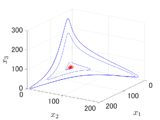
(a) Orbits in $(x_{1},x_{2},x_{3})$ space

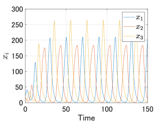
(b) Time responses (nominal)

Figure 3: Simulations: the repressilator Model

In order to investigate the robustness, we assume that there is one perturbation $\delta(s)$, which approximately represents the net effect of all the perturbations and the uncertainties in the system. This type of assumption has been made in many applications as a crude but effective approximation in robust control analysis and design using the small gain condition to avoid increased complexity in advanced methods such as $\mu$ synthesis. The target system with a multiplicative-type perturbation $\delta(s)$ is then represented as

$$\begin{array}[]{ll}\dot{x}_{1}=-\alpha_{1}x_{1}+\beta_{1}\psi_{1}(x_{3})+w,&\hskip 8.53581ptw={\hat{\delta}}z\\ \dot{x}_{2}=-\alpha_{2}x_{2}+\beta_{2}\psi_{2}(x_{1}),&\\ \dot{x}_{3}=-\alpha_{3}x_{3}+\beta_{3}\psi_{3}(x_{2}),&\\ z=\beta_{1}\psi_{1}(x_{3}),\end{array}\vspace*{-2mm}$$ (23)

where $\hat{\delta}$ is the linear operator with the input-output mapping specified by stable transfer function $\delta(s)$. The purpose of this section is to confirm the effectiveness of the theoretical results in the previous sections on the exact RIRs ($\rho_{*}$) and ($\mu_{*}$) for the repressilator. At an equilibrium, we have

$$x_{i}=\frac{\hat{\beta}_{i}}{\alpha_{i}}\psi_{i}\left(\frac{\hat{\beta}_{i-1}}{\alpha_{i-1}}\psi_{i-1}\Big{(}\frac{\hat{\beta}_{i-2}}{\alpha_{i-2}}\psi_{i-2}(x_{i})\Big{)}\right)$$ (24)

for $i=1,2,3$, where $\hat{\beta}_{1}:=(1+e)\beta_{1},$, $\hat{\beta}_{2}:=\beta_{2}$, $\hat{\beta}_{3}:=\beta_{3}$, and $e:=\delta(0)$. The right-hand side of (24) is a monotonically decreasing function in the positive orthant of $x\in\mathbb{R}^{3}$, and hence there always exists a unique equilibrium point denoted by $x_{e}=[x_{e1},x_{e2},x_{e3}]^{T}$. Figure 5 shows the change of the equilibria due to the change of $e$.

4.2 Robustness Properties

Let us first show that the repressilator model falls under our analysis framework and the robust instability radius can be calculated exactly. Noting the cyclic structure of the system, the linearization of the system around the equilibrium point is given by

$$\xi=\Big{(}1+\delta(s)\Big{)}h_{e}(s)\xi,\hskip 8.53581pt\xi:=x-x_{e},\hskip 8.53581pt$$ (25)

where

$$h_{e}(s):=\frac{-k}{(s+\alpha_{1})(s+\alpha_{2})(s+\alpha_{3})}\;,$$ (26)

$$k:=-\beta_{1}\beta_{2}\beta_{3}\psi_{1}^{\prime}(x_{e3})\psi_{2}^{\prime}(x_{e1})\psi_{3}^{\prime}(x_{e2})>0,$$ (27)

and the characteristic equation is expressed as

$$1=\delta(s)g_{e}(s),\hskip 8.53581ptg_{e}(s)=h_{e}(s)/(1-h_{e}(s)).$$ (28)

It is readily seen that $g_{e}(s)$ in (28) is represented by $g_{e}(s)=-k/(s^{3}+ps^{2}+qs+\ell)$, where $p:=\alpha_{1}+\alpha_{2}+\alpha_{3}>0$, $q:=\alpha_{1}\alpha_{2}+\alpha_{2}\alpha_{3}+\alpha_{3}\alpha_{1}>0$, and $\ell:=\alpha_{1}\alpha_{2}\alpha_{3}+k>0$. We now check inequality conditions (12) in Proposition 2 which guarantee Condition 2. We can verify that

$$\vspace*{-2mm}p^{2}-2q = (\alpha_{1}+\alpha_{2}+\alpha_{3})^{2}-2(\alpha_{1}\alpha_{2}+\alpha_{2}\alpha_{3}+\alpha_{3}\alpha_{1})$$

$$= \alpha_{1}^{2}+\alpha_{2}^{2}+\alpha_{3}^{2}>0.\vspace*{-2mm}$$

This yields $2p\ell-q^{2}>2p(pq)-q^{2}=q\{2(p^{2}-2q)+3q\}>0$. The remaining condition $\ell>pq$ implies the hyperbolic instability of $g_{e}(s)$. The maximum real part of the poles of $g_{e}(s)$ for $e\in(-1,1)$ plotted in Fig.  5 shows that $g_{e}(s)$ is hyperbolically unstable for $e\in\mathbb{E}_{h}:=(-0.94,1)$, and it can be confirmed that $\ell>pq$ holds for all $e$ in $\mathbb{E}_{h}$. Hence, we can conclude that (12) holds, which implies that conditions (a) and (b) in Lemma 4 hold as remarked just below Lemma 4. Consequently, we have $\rho_{*}(e)=\rho_{p}(e)$ for $\delta(0)=e\in\mathbb{E}_{h}\subset\mathbb{E}$, and hence we can derive the exact RIR $\mu_{*}$ by Theorem 1 or the procedure presented at the end of Section 3.3.

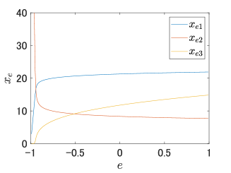
Figure 4: Equilibrium point

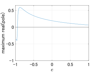
Figure 5: Maximum real part of the poles of $g_{e}(s)$

For the repressilator, the instability analysis of the equilibrium point is in fact sufficient for robustness analysis of the oscillatory behavior. A precise statement of the result is given as follows.

Proposition 3

Consider the repressilator in (23), where, with $i=1,2,3$, all the coefficients $\alpha_{i}$ and $\beta_{i}$ are positive, nonlinear functions $\psi_{i}(x)$ are bounded, continuously differentiable, and satisfy $\psi_{i}(x)>0$ and $\psi_{i}^{\prime}(x)<0$ on $x\geq 0$, and perturbation $\delta(s)$ is stable. There exists a unique equilibrium point in the positive orthant. Suppose the equilibrium is hyperbolic and unstable, and the positive orthant remains to be an invariant set in the presence of the perturbation. Then, the system is oscillatory in the sense of Yakubovich, i.e., for almost all initial states in the positive orthant, the resulting trajectory satisfies

$$\liminf_{t\rightarrow\infty}x_{i}(t)<\limsup_{t\rightarrow\infty}x_{i}(t)$$

for at least one of the state variables $x_{i}$.

Proof. The existence and uniqueness of the equilibrium point follows from (24) as discussed earlier. From (23), the dynamics of $x_{1}$ is described by

$$x_{1}=f_{1}(s)\psi_{1}(x_{3}),\hskip 8.53581ptf_{1}(s):=\beta\cdot\frac{1+\delta(s)}{s+\alpha_{1}}.$$

Since $\psi_{1}(x)$ is a bounded continuous function on $x>0$, there is a scalar $u_{1}$ such that $|\psi_{1}(x)|<u_{1}$ for all $x>0$. Due to the invariance of the positive orthant, $x_{3}(t)$ remains positive and hence $|\psi_{1}(x_{3}(t))|<u_{1}$ holds for all $t\geq 0$. Since $f_{1}(s)$ is stable, the effect of the initial condition on $x_{1}(t)$ will eventually die out and we have $|x_{1}(t)|\leq\gamma_{1}u_{1}$ for sufficiently large $t$, where $\gamma_{1}$ is the peak-to-peak gain ($L_{1}$ norm) of $f_{1}(s)$. Similar arguments apply to $x_{2}$, $x_{3}$, and the states of $\delta(s)$, and hence all the trajectories in the positive orthant are ultimately bounded. The result then follows from Theorem 1 of (Pogromsky et al., 1999).   

The invariance of the positive orthant after a perturbation is a reasonable assumption, given that the variables $x_{i}$ represent the concentration level of proteins. Hence Proposition 3 basically says that an oscillation occurs whenever the equilibrium point is unstable because every trajectory repelled from the equilibrium cannot diverge and has to stay in a bounded set regardless of the initial condition. Thus, robust instability of the equilibrium implies persistence of the oscillatory behavior. This type of analysis has been done for nominal oscillations of central pattern generators (Futakata & Iwasaki, 2008), to which our robustness analysis may also apply.

4.3 Illustration by Simulations

We first consider a simple case where the static gain of the perturbation is zero, i.e., $\delta(0)=e=0$, to confirm that $\rho_{*}(0)={\rho}_{p}(0)$ holds when $g(s)$ satisfies Condition 2 described in Section 2.4. In this case, the nominal equilibrium $x_{o}=[21.3,8.34,11.8]^{T}$ remains the same even after the perturbation, i.e., $x_{e}=x_{o}$.

Using the analytic expression in the proof of Proposition 2, the exact RIR for this system is obtained as $\rho_{*}(0)={\rho}_{p}(0)=0.4049$. We can confirm that the value is exact as long as no static gain perturbation is allowed by numerical simulations, which are not shown here due to the page limitation.

We here focus on a more realistic case where the perturbation $\delta(s)$ has a non-zero static gain $e:=\delta(0)\neq 0$. In contrast with the case of $e=0$, the equilibrium point $x_{e}$ varies with $e$ as already seen in Fig. 5. The goal is to verify Theorem 1 on the exact RIR $\mu_{*}$. To this end we use the type of plots as shown in Fig. 1. The values of $\rho_{p}(e):=1/\|g_{e}\|_{L_{\infty}}$ are plotted as a function of $e\in\mathbb{E}_{h}=(-0.94,1)$ as seen in Fig. 6. Then we have $|e|<\rho_{p}(e)$ when $-0.6027<e<0.3218$, which defines the set $\mathbb{E}_{*}$. In this interval, $g_{e}(s)$ satisfies conditions (a) and (b) in Lemma 4, and hence we conclude $\mu(e)=\rho_{p}(e)$. The smallest value within this interval $\mathbb{E}_{*}$ is $\mu(e)=0.3218$, which is the exact value of the RIR $\mu_{*}$ at the nominal equilibrium $x_{o}$ since $\mu(e)\geq|e|$ for all $e\in\mathbb{E}$, and the red lines in Fig. 6 give a lower bound on $\mu(e)$.

Figure 6: $\rho_{p}(e)$ for $g_{e}(s)$ (blue curve) and $|e|$ (red lines)

A numerical analysis by simulations depicted in Fig. 7 reconfirms that $\mu(e)$ at $e=0.3218$ gives the exact RIR $\mu_{*}$. Figure 7 (a) shows the time response for the case of

$$\vspace*{-4mm}\delta(s)=\frac{s+\xi\gamma}{s+\xi}\cdot\frac{(1+\varepsilon)b(s-a)}{s+a},\hskip 8.53581pta=2.253,\hskip 8.53581ptb=0.3218\vspace*{-4mm}$$

with $\varepsilon=0.05,\;\gamma=-0.9524,\;\xi=0.010$, where $\gamma$ is determined by $\gamma=-1/(1+\epsilon)$ to ensure that the high pass filter does not change the static gain. As illustrated in Figure 7 (a), this perturbation stabilizes $g_{e}(s)$ at $e=0.3218$ since it satisfies $\delta(0)=0.3218$ and $\|\delta\|_{H_{\infty}}=0.3379$. On the other hand, we can observe the maintenance of the periodic oscillation phenomenon if we change the sign of $\varepsilon$, meaning that the norm of $\delta(s)$ is smaller than $\mu_{*}=0.3218$ (See Fig. 7 (b)).

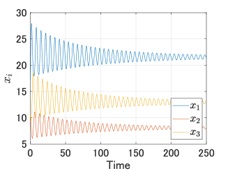
(a) Time responses (perturbed: $\varepsilon=0.05$)

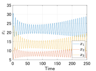
(b) Time responses (perturbed: $\varepsilon=-0.05$)

Figure 7: Simulations: Case with change of equilibrium

5 Conclusion

This paper has provided two main theoretical results on the robust instability analysis against stable perturbations. One is on the robust instability radius $\rho_{*}$ for SISO LTI systems, and the other is on the robust instability radius $\mu_{*}$ for parametrized LTI systems. The effectiveness of the theoretical results has been illustrated by numerical simulations of the repressilator model. This example demonstrated that the theoretical quantitative foundation provided in this paper based on the local stability/instability property can lead to a useful tool in the field of synthetic biology.

The classic theory (Pogromsky et al., 1999) guarantees existence of oscillations which may not be periodic under instability of equilibrium points and ultimate boundedness of trajectories. However, periodic orbits may serve better for functional purposes in applications. A recent result on the analysis of global nonlinear behaviors based on the concept of $p$-Dominance (Forni & Sepulchre, 2019) may be useful to guarantee persistence of a limit cycle for a class of systems. Toward this direction, our quantitative tool for the instability analysis may be effective for checking the $p$-Dominance condition through the spectral splitting.

The future work along this research direction includes a characterization of higher order systems for which the RIR can be analyzed exactly and its applications to a more general type of biomolecular systems.

Acknowledgments:   The authors would like to thank Chung-Yao Cao for his valuable comments to improve the paper. This work was supported in part by the Ministry of Education, Culture, Sports, Science and Technology in Japan through Grant-in-Aid for Scientific Research (A) 21246067 and (B) 18H01464.

Appendix A Proof of Proposition 1

Let $\delta_{o}(s)$ and $g(s)$ be expressed as the ratios of coprime polynomials $\delta_{o}(s)=b_{o}(s)/a_{o}(s)$ and $g(s)=n(s)/d(s)$, respectively. Here, $\delta_{o}(s)$ may be a real constant with $b_{o}\in\mathbb{R}$ and $a_{o}=1$. Let $b_{1}(s)$ and $a_{1}(s)$ be coprime polynomials of the same degree. For $\delta_{1}(s):=b_{1}(s)/a_{1}(s)$, the characteristic polynomial of the perturbed closed-loop system is given by $p(s)=\varepsilon q(s)$ with $p(s):=(a_{o}(s)d(s)-b_{o}(s)n(s))a_{1}(s),$ and $q(s):=a_{o}(s)b_{1}(s)n(s)$. Since $\delta_{o}(s)$ marginally stabilizes $g(s)$ with a simple pole on the imaginary axis (denote it by $s=j\omega_{c}$, where $\omega_{c}$ may be zero), the nominal characteristic polynomial $p(s)$ takes the form $p(s)=(s-j\omega_{c})\hat{p}(s)$, where $\hat{p}(j\omega_{c})\neq 0$. Hence, the characteristic equation can be written as $s-j\omega_{c}=\varepsilon r(s),\hskip 8.53581ptr(s):=q(s)/\hat{p}(s)$.

We apply the root locus method and focus on the direction of the root locus around $s=j\omega_{c}$ when $\varepsilon$ varies between negative and positive values. For small perturbation $|\varepsilon|$, consider the characteristic root $\lambda_{\varepsilon}$ that passes through $j\omega_{c}$ at $\varepsilon=0$. Note that $\angle(\lambda_{\varepsilon}-j\omega_{c})=\angle r(\lambda_{\varepsilon})+\angle(\varepsilon)$ holds for the phase angles. Taking the limit $\varepsilon\rightarrow 0$,

$$\vspace*{-2mm}\angle(\lambda_{\varepsilon}-j\omega_{c})\rightarrow\left\{\begin{array}[]{ll}\angle r(j\omega_{c}),&(\varepsilon\downarrow 0),\\ \angle r(j\omega_{c})+\pi,&(\varepsilon\uparrow 0),\end{array}\right.\vspace*{-2mm}$$

where the limit is well defined due to $r(j\omega_{c})\neq 0$, which is verified as follows. Note that $r(j\omega_{c})=0$ implies $a_{o}(j\omega_{c})b_{1}(j\omega_{c})n(j\omega_{c})=0$. For a generic $b_{1}(s)$, we have $b_{1}(j\omega_{c})\neq 0$. Since $\delta_{o}(s)$ has no pole on the imaginary axis, $a_{o}(j\omega_{c})\neq 0$. Thus we conclude $n(j\omega_{c})=0$. Since $s=j\omega_{c}$ is a pole of the nominal closed-loop system with $\varepsilon=0$, we have $b_{o}(j\omega_{c})n(j\omega_{c})=a_{o}(j\omega_{c})d(j\omega_{c})=0$. However, this is a contradiction since $\delta_{o}(s)$ has no pole on the imaginary axis and $(n,d)$ are coprime. Thus $r(j\omega_{c})$ must be nonzero. Now, we may assume, for a generic $\delta_{1}(s)$, that the real part of $r(j\omega_{c})$ is nonzero and $\angle r(j\omega_{c})\neq\pm\pi/2$. Since the phase angle of $\lambda_{\varepsilon}-j\omega_{c}$ rotates by $\pi$ when passing through $\varepsilon=0$, we see that $\lambda_{\varepsilon}$ has a negative real part when $\varepsilon>0$ or $\varepsilon<0$. If $|\varepsilon|$ is sufficiently small, the other characteristic roots will stay in the OLHP. Thus we conclude the result.

Appendix B Proof of Proposition 2

The proof of the first part is easy. The requirement of the odd number of the ORHP poles of $g(s)$ is equivalent to $\ell<0$. For a constant $\delta$, the closed-loop characteristic equation is given by $s^{3}+ps^{2}+(q-\delta\zeta)s+(\ell+k\delta)=0$. When $\delta=-\ell/k$, one root is at the origin, and the remaining two roots are in the OLHP if and only if $p>0$ and $q-\delta\zeta=q+\zeta\ell/k>0$. Thus we have (11).

Now we define $\psi(s):=1/g(s)$ for the proof of the second part. Letting $\Omega:=\omega^{2}$, $|\psi(j\omega)|^{2}$ is given by

$$\vspace*{-2mm}F(\Omega):=(\Omega^{3}+f_{2}\Omega^{2}-f_{1}\Omega+f_{0})/(\zeta^{2}\Omega+k^{2}),\vspace*{-2mm}$$ (29)

where $f_{2}:=p^{2}-2q$, $f_{1}:=2p\ell-q^{2}>0$, and $f_{0}:=\ell^{2}>0$. We now seek the critical frequency $\omega_{p}$ which provides the minimum of $F(\Omega)$ by calculating $dF(\Omega)/d\Omega$. It is seen that $dF(\Omega)/d\Omega=0$ is equivalent to

$$\vspace*{-2mm}H(\Omega) := 2\zeta^{2}\Omega^{3}+(\zeta^{2}f_{2}+3k^{2})\Omega^{2}$$ (30)

$$+2k^{2}f_{2}\Omega-(\zeta^{2}f_{0}+k^{2}f_{1})=0.\vspace*{-2mm}$$

We show that $H(\Omega)$ has a unique positive solution $\Omega_{p}$ which corresponds to the critical frequency $\omega_{p}^{2}\neq 0$. First note that $f_{0}>0$ and $f_{1}>0$ imply $H(0)<0$. $dH(\Omega)/d\Omega$ is positive for all $\Omega>0$ if $f_{2}\geq 0$ and $dH(\Omega)/d\Omega$ at $\Omega=0$ is negative if $f_{2}<0$ . These facts conclude that $H(\Omega)$ has a unique positive solution $\Omega_{p}$.

Hereafter we will show that $\delta_{o}(s)$ defined by (8) marginally stabilizes $g(s)$, which means that the characteristic equation $1-\delta_{o}(s)g(s)=0$, or

$$\vspace*{-2mm}(s^{3}+ps^{2}+qs+\ell)(s+a)-b(\zeta s-k)(s-a)=0\vspace*{-2mm}$$ (31)

has a form of

$$\vspace*{-2mm}(s^{2}+\Omega_{p})(s^{2}+\sigma_{1}s+\sigma_{0})=0\vspace*{-2mm}$$ (32)

for a certain positive parameters $\sigma_{1}$ and $\sigma_{0}$. Comparing the coefficients of (31) and (32), we have

$${\bf A}{\bf x}={\bf b},\hskip 8.53581pt{\bf x}:=\left[\begin{array}[]{ccc}a&\sigma_{1}&\sigma_{0}\end{array}\right]^{T},$$ (34)

$${\bf A}:=\left[\begin{array}[]{ccc}-1&1&0\\ -p&0&1\\ -(q+\zeta b)&\Omega_{p}&0\\ kb-\ell&0&\Omega_{p}\end{array}\right],\hskip 8.53581pt{\bf b}:=\left[\begin{array}[]{c}p\\ q-\zeta b-\Omega_{p}\\ \ell+kb\\ 0\end{array}\right].\vspace*{-2mm}$$ (43)

It is clear that $\mbox{rank}\;{\bf A}=3$ and that ${\bf A_{b}}:=\left[\begin{array}[]{cc}{\bf A}&{\bf b}\end{array}\right]$ is singular because the determinant of ${\bf A_{b}}$ is equal to $(\zeta^{2}\Omega_{p}+k^{2})(F(\Omega_{p})-b^{2})=0$. This guarantees the existence of the unique solution of (34).

Consequently, the remaining step of the proof is to show the positivity of the solution ${\bf x}$, i.e., $a>0$, $\sigma_{1}>0$, and $\sigma_{0}>0$. Note that $b$ defined in (9) for $\omega_{c}=\omega_{p}$ satisfies

$$\vspace*{-2mm}|b|=1/\max_{\omega\neq 0}|g(j\omega)|=\min_{\omega\neq 0}|\psi(j\omega)|<\ell/|k|=|\psi(0)|\vspace*{-2mm}$$

and that $a$ can always be chosen to be positive, depending on the sign of $b$ as described in (9).

Under the assumptions of $a>0$ and $|kb|<\ell$ with $p>0$, the 1st and the 4th rows in (34) yield $\sigma_{1}=a+p>0$ and $\sigma_{0}=(\ell-kb)a/\Omega_{p}>0$, respectively. This completes the proof of the second part.

Appendix C Proofs of Lemmas 2, 3, and 4

$\bullet$ Proof of Lemma 2

The first condition $\mu(e)\geq|e|$ follows from the definition of $\mu(e)$ in (14) because $\|\delta\|_{H_{\infty}}\geq|\delta(0)|=|e|$ for $\delta(s)\in\Delta_{e}$. In the second condition, we obtain $\mu(e)\geq\rho_{*}(e)$ by inspection of (15).

$\bullet$ Proof of Lemma 3

The characteristic equation in (17) can be rewritten as

$$1+\frac{\xi}{s}L(s)=0,\hskip 8.53581ptL(s):=\frac{1-\gamma\ell(s)}{1-\ell(s)}.$$ (44)

Note that $L(s)$ is stable since $1=\ell(s)$ implies $\Re(s)<0$. We claim that $L(s)$ has an even number of zeros (including multiplicities) in the ORHP and no zeros on the imaginary axis. This is easy to see for the case $\gamma=0$ because the zeros of $L(s)$ coincide with the poles of $\ell(s)$. When $\gamma\neq 0$, by the small gain condition in (16), $1=\gamma_{o}\ell(s)$ has no roots on the imaginary axis for all $\gamma_{o}$ such that $|\gamma_{o}|\leq|\gamma|$. Since $\ell(s)$ has an even number of poles in the ORHP and no poles on the imaginary axis, there are even number of roots of $1=\gamma_{o}\ell(s)$ in the ORHP when $|\gamma_{o}|$ is nonzero and sufficiently small. As $|\gamma_{o}|$ increases to $|\gamma|$, none of the roots of $1=\gamma_{o}\ell(s)$ can go across the imaginary axis, and hence $1=\gamma\ell(s)$ has an even number of ORHP roots. Thus $L(s)$ has no zero on the imaginary axis and an even number of zeros in the ORHP. Then the root locus shows that all the roots of the characteristic equation in (44) are in the OLHP for sufficiently small $\xi>0$.

$\bullet$ Proof of Lemma 4

Let $\delta_{e}(s)$ be a transfer function as described in (a). Then a slight perturbation of $\delta_{e}(s)$ can stabilize $g_{e}(s)$ as shown in Proposition 1. That is, for an arbitrarily small $\varepsilon>0$, there exists a stable transfer function $\tilde{\delta}_{e}(s)$ that stabilizes $g_{e}(s)$ and satisfies $\|\delta_{e}-\tilde{\delta}_{e}\|_{H_{\infty}}<\varepsilon$. Now, the static gain of the perturbation $\tilde{\delta}_{e}(s)$ is approximately given by $\tilde{\delta}_{e}(0)\cong\delta_{e}(0)=\rho_{p}(e)$, and hence this perturbation may not belong to $\Delta_{e}$. Let the static gain of the perturbation be adjusted by a high pass filter

$$\vspace*{-2mm}\delta(s):=f(s)\tilde{\delta}_{e}(s),\hskip 8.53581ptf(s):=\frac{s+\xi\gamma}{s+\xi},\hskip 8.53581pt\gamma:=\frac{e}{\tilde{\delta}_{e}(0)},\vspace*{-2mm}$$

so that $\delta(0)=e$. We will show that $\delta(s)$ with sufficiently small $\xi>0$ stabilizes $g_{e}(s)$ and hence $\delta(s)\in\Delta_{e}$, using Lemma 3 with $\ell(s):=\tilde{\delta}_{e}(s)g_{e}(s)$, where the characteristic equation $1=\delta(s)g_{e}(s)$ is given by (17). First note that $\ell(s)$ has an even number of poles in the ORHP and no poles on the imaginary axis because $g_{e}(s)$ is hyperbolic and satisfies condition (b), and $\tilde{\delta}_{e}(s)$ is stable. Next, all the roots of $1=\ell(s)$ are in the OLHP since $\tilde{\delta}_{e}(s)$ stabilizes $g_{e}(s)$. Also note that $|\gamma|<1=\|f\|_{H_{\infty}}$ for all $\xi>0$ since $|\tilde{\delta}_{e}(0)|\cong\rho_{p}(e)$ and $|e|<\rho_{p}(e)$, and hence $\|\delta\|_{H_{\infty}}\cong\rho_{p}(e)$. Moreover, we have $\|\gamma\ell\|_{L_{\infty}}<1$ because

$$\vspace*{-2mm}\|\gamma\tilde{\delta}_{e}\|_{H_{\infty}}=|e|\cdot\frac{\|\tilde{\delta}_{e}\|_{H_{\infty}}}{|\tilde{\delta}_{e}(0)|}<\rho_{p}(e)\vspace*{-2mm}$$ (45)

holds, where the inequality follows from the fact that $\|\tilde{\delta}_{e}\|_{H_{\infty}}/|\tilde{\delta}_{e}(0)|$ is arbitrarily close to $1$ because $\delta_{e}(s)$ is all pass and $\|\tilde{\delta}_{e}-\delta_{e}\|_{H_{\infty}}$ is arbitrarily small. Thus, all the conditions in Lemma 3 are satisfied and we conclude that $\delta(s)$ with sufficiently small $\xi>0$ stabilizes $g_{e}(s)$ and hence $\delta(s)\in\Delta_{e}$. The proof is now complete by noting that $\mu(e)\leq\|\delta\|_{H_{\infty}}\cong\rho_{p}(e)$ due to the preceding argument and $\rho_{p}(e)\leq\mu(e)$ due to Lemma 2.

References

- (1)
- Alon (2006) Alon, U. (2006), An Introduction to Systems Biology: Design Principles of Biological Circuits, Chapman and Hall/CRC.
- Elowitz & Leibler (2000) Elowitz, M. & Leibler, S. (2000), ‘A synthetic oscillatory network of transcriptional regulators’, Nature 403(6767), 335–338.
- Forni & Sepulchre (2019) Forni, F. & Sepulchre, R. (2019), ‘Differential dissipativity theory for dominance analysis’, IEEE Trans. Auto. Contr. 64(6), 2340–2351.
- Futakata & Iwasaki (2008) Futakata, Y. & Iwasaki, T. (2008), ‘Formal analysis of resonance entrainment by central pattern generator’, J. Math. Biol. 57(2), 183–207.
- Grizzle et al. (2001) Grizzle, J., Abba, G. & Plestan, F. (2001), ‘Asymptotically stable walking for biped robots: analysis via systems with impulse effects’, IEEE Trans. Auto. Contr. 46(1), 51–64.
- Hara et al. (2020) Hara, S., Iwasaki, T. & Hori, Y. (2020), ‘Robust instability analysis with neuronal dynamics’, Proc. IEEE Conf. Dec. Contr. .
- Hinrichsen & Pritchard (1986) Hinrichsen, D. & Pritchard, A. (1986), ‘Stability radii of linear systems’, Sys. Contr. Lett. 7, 1–10.
- Hori et al. (2011) Hori, Y., Kim, T. & Hara, S. (2011), ‘Existence criteria of periodic oscillations in cyclic gene regulatory networks’, Automatica (Special Issue on Systems Biology) 47(6), 1203–1209.
- Inoue et al. (2013a) Inoue et al., M. (2013a), ‘An instability condition for uncertain systems toward robust bifurcation analysis’, Proc. Euro. Contr. Conf. pp. 3264–3269.
- Inoue et al. (2013b) Inoue et al., M. (2013b), ‘Robust bifurcation analysis based on the nyquist stability criterion’, Proc. IEEE Conf. Dec. Contr. pp. 1768–1773.
- Inoue et al. (2015) Inoue et al., M. (2015), ‘Absolute instability of lur’e systems and its application to oscillation analysis of uncertain genetic networks’, Int. J. Rob. Nonlin. Contr. 25, 3746–3762.
- Niederholtmeyer et al. (2015) Niederholtmeyer et al., H. (2015), ‘Rapid cell-free forward engineering of novel genetic ring oscillators’, eLife 4, e09771.
- Pogromsky et al. (1999) Pogromsky, A., Glad, T. & Nijmeijer, H. (1999), ‘On diffusion driven oscillations in coupled dynamical systems’, Int. J. Bifurcation and Chaos 9(4), 629–644.
- Potvin-Trottier et al. (2016) Potvin-Trottier, L., Lord, N., Vinnicombe, G. & Paulsson, J. (2016), ‘Synchronous long-term oscillations in a synthetic gene circuit’, Nature 538(7626), 514–517.
- Wada et al. (1998) Wada et al., T. (1998), ‘Parametric absolute stability of lur’e systems’, IEEE Trans. Auto. Contr. 43(11), 1649–1653.
- Wada et al. (2000) Wada et al., T. (2000), ‘Parametric absolute stability of multivariable lur’e systems’, Automatica 36(9), 1365–1372.
- Wu & Iwasaki (2021) Wu, A. & Iwasaki, T. (2021), ‘Design of controllers with distributed CPG architecture for adaptive oscillations’, Int. J. Robust and Nonlin. Contr. 31(2), 694–714.
- Youla et al. (1974) Youla, D., Jr., J. B. & Lu, C. (1974), ‘Single-loop feedback-stabilization of linear multivariable dynamical plants’, Automatica 10, 159–173.