Self-supporting wormholes with massive vector field

Abstract

In this paper we consider a massive vector field in the background of a space-time obtained by certain $\mathbb{Z}_{2}$ quotient of the BTZ black hole. We analyse the back reaction of the matter field on the space-time geometry up to first order in metric perturbation. The expectation value of the stress-energy tensor can be computed exactly by considering its pull-back onto the covering space. Upon a suitable choice of the boundary condition on the vector field around a non-contractible cycle of the quotient manifold it is possible to obtain the average energy on a null geodesic to be negative there by resulting a traversable wormhole.

1 Introduction

Wormholes are solutions to Einstein equations which connect two otherwise distinct space-times or two widely separated regions of the same space-time via a throat. In classical general relativity wormholes are not traversable, i.e., no causal curve can pass through the throat of the wormhole connecting the two distinct regions. The issue of traversability for static, spherically symmetric wormholes has been discussed first in [1] where it has been pointed out the need to have exotic matters for the wormhole to be traversable. This matter has further been analysed in [2, 3, 4] substantiating the violation of average null energy condition (ANEC) as the necessary condition for traversability of wormhole. It has been proved that the ANEC holds for achronal null geodesics [5, 6, 7]. Thus, space-times which possess only achronal null geodesics do not admit traversable wormholes. These results have their origin lies in the topological censorship theorem [8] and its generalisation to asymptotically locally anti-de Sitter spaces [9], which states that every causal curve whose end points lie in the boundary at infinity (${\cal I}$) can be deformed to a causal curve which entirely lies in $\cal I$ itself.

An important breakthrough in this direction has recently been achieved by Gao, Jafferis and Wall [10] where they have constructed a traversable wormhole from an eternal BTZ black hole by introducing a time-dependent coupling between its two asymptotic regions. They have computed the one loop stress energy tensor upon using the point splitting method. By choosing the sign of the coupling appropriately the vacuum expectation value of the double null component of the stress energy tensor can be made negative enabling the wormhole traversable. These results have subsequently been generalised in [11] to see the effect of rotation on the size of the wormhole. An eternal traversable wormhole in nearly-$AdS_{2}$ space-time has been constructed in [12] by introducing a coupling between the two boundaries.

A traversable wormhole in four dimensions has been devised in [13] by joining the throats of two charged extremal black hole geometries in the presence of massless fermions. This construction did not depend on any non-local external coupling between the two boundaries and resulted to what are called as the self-supporting wormholes which arise entirely from local dynamics of the fermion fields present in the bulk of the space-time. A complementary analysis has been carried out in [14] to obtain traversable wormholes from the bulk dynamics by considering a free scalar field in quotients of $AdS_{3}$ and $AdS_{3}\times S^{1}$ by discreet symmetries. The authors computed the gravitational back reaction and showed that the space-time admits causal curves which can’t be deformed to the boundary. Taking quotient by a discrete symmetry is significant in the sense that, it no longer preserves the globally defined Killing field which plays a key role in obtaining the average null energy condition. This result has subsequently been generalised [15] to include fermions in the bulk to produce traversable wormholes.

In the present work we generalise these above results in the presence of massive vector fields. As has been noticed in [15], adding spin-half fields provide a rich structure which is worth studying in its own right. We will notice similar phenomenon in the presence of spin-one fields. In what follows, we consider the pullback of the stress tensor on to the covering space. For $AdS_{3}$ it is possible to obtain an exact analytic expression for the propagator in closed form. Using this result we compute the expectation value of the stress tensor and show that under imposing suitable boundary conditions, this gives rise to traversable wormholes. The plan of the paper is as follows. The next section summarises the preliminaries on obtaining self-supporting wormholes from free scalar fields. In §3 we obtain the exact propagator in $AdS_{3}$. Subsequently we compute the expectation value of the stress tensor from this propagator by using the method of images. The appendix discusses some of the technical details.

2 Preliminaries

Consider the $AdS_{3}$ metric in Kruskal-like coordinates:

$$dS^{2}=\frac{1}{\left(1+UV\right)^{2}}\Big{(}-4\ell^{2}dUdV+r_{+}^{2}\left(1-UV\right)^{2}d\varphi^{2}\Big{)}\ .$$ (2.1)

This gives rise to non-rotating BTZ black hole with horizon radius $r_{+}$ upon imposing the identification $\varphi\sim\varphi+2\pi$ for the azimuthal angle. The horizons of the black hole are located at $U=0$ and $V=0$ respectively. The space-time boundaries correspond to $1+UV=0$. This solution has been discussed from the perspective of gauge-gravity duality in [16]. The issue of traversability in this geometry has been analysed first in [10] by considering a relevant double trace deformation coupling the two boundaries. This relevant deformation in the boundary CFT amounts to adding a stress tensor in the bulk resulting a perturbation of the space-time geometry.

Consider the $V=0$ horizon which admits the horizon generator $k^{\rho}$ such that $k^{\rho}\partial_{\rho}=\partial_{U}$. We choose $U$ to be the affine parameter which parametrises the null geodesics tangent to this horizon. The linearised Einstein’s equation for the metric perturbation on the $V=0$ horizon is given by:

$$\frac{1}{2\ell^{2}}\left(h_{UU}+\partial_{U}(Uh_{UU})-\frac{\ell^{2}}{r_{+}^{2}}\partial_{U}^{2}h_{\varphi\varphi}\right)=8\pi G_{N}T_{UU}\ .$$ (2.2)

The geodesic equation for null rays originating on the past horizon on the other hand gives rise to

$$\Delta V(U)=\frac{1}{2\ell^{2}}\int_{-\infty}^{U}dU\ h_{UU}\ .$$ (2.3)

The quantity $\Delta V(\infty)$ measures the time delay of the null geodesic starting at $U=-\infty$ and ending at $U=\infty$. The wormhole becomes traversable if $\Delta V(\infty)<0$. This quantity provides a measure for the size of the opening of the wormhole. Integrating (2.2) over $U$ keeping in mind the perturbation vanish at the boundary gives rise to

$$\Delta V(\infty)=8\pi G_{N}\int_{-\infty}^{\infty}dU\ T_{UU}\ .$$ (2.4)

Thus the wormhole becomes traversable if the ANEC is violated. By choosing suitable non-local coupling between the two boundaries it has been shown [10] that it is indeed possible to violate the ANEC giving rise to traversable wormholes.

An alternative method has been developed in [14] to construction traversable wormholes without invoking any non-local boundary interaction. The authors considered a suitable $\mathbb{Z}_{2}$ quotient of the $BTZ$ black hole space-time $\tilde{M}$. The resulting geometry $M$ is a smooth, globally hyperbolic manifold, known as the $\mathbb{RP}^{2}$-geon [17]. The $\mathbb{Z}_{2}$ quotient introduces a new homotopy cycle in the manifold $M$. One can choose the scalar field in $M$ to be either periodic or anti-periodic around this cycle. The states in $M$ are constructed from the states of the covering space $\tilde{M}$ by the method of images. This enables the average expectation value in a suitable Hartle-Hawking like state of the double null component of the resulting stress tensor to take negative values along null geodesics.

Let $J$ be the isometry which maps the point $\tilde{x}\in\tilde{M}$ to $J\tilde{x}$, and the pair $(\tilde{x},J\tilde{x})$ projects onto the point $x$ in the quotient $M$. The quantum fields $\phi_{\pm}(x)$ in $M$ are constructed from the quantum fields $\tilde{\phi}(\tilde{x})$ in $\tilde{M}$ using the method of images:

$$\phi_{\pm}(x)=\frac{1}{\sqrt{2}}\Big{(}\tilde{\phi}(\tilde{x})\pm\tilde{\phi}(J\tilde{x})\Big{)}\ .$$ (2.5)

The pair of points $(\tilde{x},J\tilde{x})$ are space-like separated in $\tilde{M}$ and hence the fields at these two points commute with each other. Thus, the fields $\phi_{\pm}(x)$ satisfies the usual canonical commutation relations and describe well defined quantum fields in $M$.

We consider free scalar field $\phi_{\pm}(x)$ in $M$ for which the action is given by

$$S=\int d^{3}x\sqrt{-g}\left(-\frac{1}{2}g^{\mu\nu}\partial_{\mu}\phi_{\pm}\partial_{\nu}\phi_{\pm}-\frac{1}{2}m^{2}\phi_{\pm}^{2}\right)\ ,$$ (2.6)

with the corresponding energy-momentum tensor

$$T_{\mu\nu\pm}=\partial_{\mu}\phi_{\pm}\partial_{\nu}\phi_{\pm}-\frac{1}{2}g_{\mu\nu}\left(g^{\alpha\beta}\partial_{\alpha}\phi_{\pm}\partial_{\beta}\phi_{\pm}+m^{2}\phi_{\pm}^{2}\right)\ .$$ (2.7)

The Hartle-Hawking state $|HH,\tilde{M}\rangle$ in the covering space $\tilde{M}$ induces corresponding states $|HH,\pm\rangle$ in $M$. We need to compute the expectation value of the double null component of the stress tensor $\langle HH,\pm|T_{\mu\nu}k^{\mu}k^{\nu}(x)|HH,\pm\rangle$ in the Hartle-Hawking states $|HH,\pm\rangle$. It is most convenient to compute this by considering the pullback $T^{P}_{\mu\nu}(\tilde{x})$ in $\tilde{M}$ of the stress-tensor $T_{\mu\nu}(x)$:

$$\langle HH,\pm|T_{\mu\nu\pm}k^{\mu}k^{\nu}(x)|HH,\pm\rangle=\langle HH,\tilde{M}|T^{P}_{\mu\nu\pm}k^{\mu}k^{\nu}(\tilde{x})|HH,\tilde{M}\rangle\ .$$ (2.8)

It is important to note that $T^{P}_{\mu\nu}(\tilde{x})$ is not the stress-tensor of a free quantum field $\tilde{\phi}(\tilde{x})$ in $\tilde{M}$. Since the Hartle-Hawking state $|HH,\tilde{M}\rangle$ is invariant under the Killing symmetry, the expectation value of the stress tensor $\tilde{T}_{\mu\nu}(\tilde{x})$ in this state vanishes. This is because, the expectation value of $\xi^{\mu}\xi^{\nu}\tilde{T}_{\mu\nu}(\tilde{x})$ is invariant for a Killing vector $\xi^{\mu}$. If $\xi^{\mu}$ becomes $k^{\mu}$ on the horizon then this quantity vanishes on the bifurcation surface, and hence the expectation value of the double null component of the stress tensor for the covering space must vanish identically. However, this need not be the case for the pullback $T^{P}_{\mu\nu}(\tilde{x})$, as this quantity is not preserved by the Killing symmetry. A straightforward analysis gives rise to

$$T^{P}_{\mu\nu\pm}k^{\mu}k^{\nu}(\tilde{x})=\tilde{T}_{\mu\nu}k^{\mu}k^{\nu}(\tilde{x})\pm k^{\mu}\partial_{\mu}\tilde{\phi}(\tilde{x})k^{\nu}\partial_{\nu}\tilde{\phi}(J\tilde{x})\ .$$ (2.9)

Thus, we have

$$\langle HH,\pm|T_{\mu\nu\pm}k^{\mu}k^{\nu}(x)|HH,\pm\rangle=\pm\langle HH,\tilde{M}|k^{\mu}\partial_{\mu}\tilde{\phi}(\tilde{x})k^{\nu}\partial_{\nu}\tilde{\phi}(J\tilde{x})|HH,\tilde{M}\rangle\ .$$ (2.10)

Hence, if the expectation value on the right hand side is non-zero, we can always choose appropriate boundary condition to make it negative. This has been computed for various smooth, globally hyperbolic, $\mathbb{Z}_{2}$ quotients of $BTZ$ and $BTZ\times S^{1}$ space-times [14]. The results have been used thereafter to show the violation of ANEC.

3 The massive vector fields

We will now consider the case of an Abelian vector field of mass $m$ with the action

$$S=\int d^{3}x\sqrt{-g}\left(-\frac{1}{4}g^{\alpha\beta}g^{\mu\nu}F_{\alpha\mu}F_{\beta\nu}-\frac{1}{2}m^{2}g^{\mu\nu}A_{\mu}A_{\nu}\right)$$ (3.1)

As in the case of scalar fields, we can use the method of images to set the vector field $A_{\mu}(x)$ in $M$, in terms of the corresponding fields $\tilde{A}_{\mu}(\tilde{x})$ in the covering space $\tilde{M}$ as:

$$A_{\mu}^{\pm}(x)=\frac{1}{\sqrt{2}}\Big{(}\tilde{A}_{\mu}(\tilde{x})\pm\tilde{A}_{\mu^{\prime}}(\tilde{x}^{\prime})\Big{)}\ .$$ (3.2)

The $(\pm)-$sign in the superscript correspond to the choice of periodic or anti-periodic boundary condition on the vector field $A_{\mu}(x)$ around the non-trivial homology cycle $\gamma$. The above setting will give rise to a well defined quantum field in $M$ for space-like separated points $(\tilde{x},\tilde{x}^{\prime})$. Here we will set $\tilde{x}^{\prime}=J\tilde{x}$. The pair of points $(\tilde{x},J\tilde{x})$ in $\tilde{M}$ maps onto the point $x\in M$ under the action of $\mathbb{Z}_{2}$.

The stress tensor corresponding to the action (3.1) is given by

$$T_{\mu\nu}^{\pm}(x)=g^{\alpha\beta}F_{\alpha\mu}^{\pm}F_{\beta\nu}^{\pm}+m^{2}A_{\mu}^{\pm}A_{\nu}^{\pm}-g_{\mu\nu}\left(\frac{1}{4}g^{\alpha\beta}g^{\rho\sigma}F_{\alpha\rho}^{\pm}F_{\beta\sigma}^{\pm}+\frac{1}{2}m^{2}g^{\alpha\beta}A_{\alpha}^{\pm}A_{\beta}^{\pm}\right)\ .$$ (3.3)

The last term in the above equation does not contribute to the double null component of $T_{\mu\nu}$. Hence, we will ignore this term now on. The pullback of the first two terms into the covering space $\tilde{M}$ gives rise to

$$k^{\mu}k^{\nu}T^{\pm}_{\mu\nu}(x)=\frac{1}{2}\Big{(}k^{\mu}k^{\nu}\tilde{T}_{\mu\nu}(\tilde{x})+k^{\mu^{\prime}}k^{\nu^{\prime}}\tilde{T}_{\mu^{\prime}\nu^{\prime}}(\tilde{x}^{\prime})\Big{)}\pm\frac{1}{2}\left\{\Big{(}g^{\alpha\beta^{\prime}}(\tilde{x},\tilde{x}^{\prime})k^{\mu}\tilde{F}_{\alpha\mu}(\tilde{x})k^{\nu^{\prime}}\tilde{F}_{\beta^{\prime}\nu^{\prime}}(\tilde{x}^{\prime})\right.$$ (3.4)

$$+\left.g^{\alpha^{\prime}\beta}(\tilde{x}^{\prime},x)k^{\mu^{\prime}}\tilde{F}_{\alpha^{\prime}\mu^{\prime}}(\tilde{x}^{\prime})k^{\nu}\tilde{F}_{\beta\nu}(\tilde{x})\Big{)}+m^{2}\Big{(}k^{\mu}\tilde{A}_{\mu}(\tilde{x})k^{\nu^{\prime}}\tilde{A}_{\nu^{\prime}}(\tilde{x}^{\prime})+k^{\mu^{\prime}}\tilde{A}_{\mu^{\prime}}(\tilde{x}^{\prime})k^{\nu}\tilde{A}_{\nu}(\tilde{x})\Big{)}\right\}.$$ (3.5)

Here $\tilde{T}_{\mu\nu}(\tilde{x})$ is the stress tensor corresponding to the gauge field $\tilde{A}_{\mu}(\tilde{x})$ in $\tilde{M}$. The expectation values of $T_{\mu\nu}(x)$ in the states $|HH,\pm\rangle$ become

$$\langle HH,\pm|k^{\mu}k^{\nu}T^{\pm}_{\mu\nu}(x)|HH,\pm\rangle = \pm\left\{\langle HH,\tilde{M}|\Big{(}g^{\alpha\beta^{\prime}}(\tilde{x},\tilde{x}^{\prime})k^{\mu}\tilde{F}_{\alpha\mu}(\tilde{x})k^{\nu^{\prime}}\tilde{F}_{\beta^{\prime}\nu^{\prime}}(\tilde{x}^{\prime})\Big{)}|HH,\tilde{M}\rangle\right.$$ (3.6)

$$+ \left.m^{2}\langle HH,\tilde{M}|\Big{(}k^{\mu}\tilde{A}_{\mu}(\tilde{x})k^{\nu^{\prime}}\tilde{A}_{\nu^{\prime}}(\tilde{x}^{\prime})\Big{)}|HH,\tilde{M}\rangle\right\}\ .$$ (3.7)

The expectation value $\langle HH,\tilde{M}|k^{\mu}k^{\nu}\tilde{T}_{\mu\nu}(\tilde{x})|HH,\tilde{M}\rangle$ vanishes because of symmetry as argued in the previous section. Again, as in the scalar field case, we can impose appropriate boundary conditions on the vector field to make the null energy negative provided the right hand side in (3.6) does not vanish.

3.1 The propagator

From the above analysis we find that, in order to verify the ANEC, we need to compute the expectation values $\langle HH,\tilde{M}|\tilde{A}_{\mu}(\tilde{x})\tilde{A}_{\nu^{\prime}}(\tilde{x}^{\prime})|HH,\tilde{M}\rangle$ and $\langle HH,\tilde{M}|\tilde{F}_{\alpha\mu}(\tilde{x})F_{\beta^{\prime}\nu^{\prime}}(\tilde{x}^{\prime})|HH,\tilde{M}\rangle$ in the covering space $\tilde{M}$. The manifold $\tilde{M}$ itself can be obtained upon taking the quotient of $AdS_{3}$ with the identification $\varphi\sim\varphi+2\pi$. Thus, we can derive these quantities from the vector two-point function in $AdS_{3}$.

The vector two-point function in $AdS_{n}$ in arbitrary dimensions has been computed in [18]. In the following we will briefly outline the relevant parts of their results for our purpose. Denote $A_{\mu}(x)$ to be the massive vector field in $AdS_{n}$. The two-point function $Q_{\mu\nu^{\prime}}(x,x^{\prime})=\langle A_{\mu}(x)A_{\nu^{\prime}}(x^{\prime})\rangle$ evaluated on the vacuum is a maximally symmetric bitensor in $AdS_{n}$. On general grounds it can be express as

$$Q_{\alpha\beta^{\prime}}(x,x^{\prime})=\upalpha(\upmu)g_{\alpha\beta^{\prime}}(x,x^{\prime})+\upbeta(\upmu)n_{\alpha}(x,x^{\prime})n_{\beta^{\prime}}(x,x^{\prime})\ .$$ (3.8)

Here $\upmu(x,x^{\prime})$ is the geodesic distance between the points $x$ and $x^{\prime}$, the unit vectors $n_{\alpha}$ and $n_{\alpha^{\prime}}$ are the covariant derivatives of $\upmu$ with respect to $x^{\alpha}$ and $x^{\alpha^{\prime}}$ respectively:

$$n_{\alpha}(x,x^{\prime})=\nabla_{\alpha}\upmu(x,x^{\prime})\ ,\ n_{\alpha^{\prime}}=\nabla_{\alpha^{\prime}}\upmu(x,x^{\prime})\ ,$$ (3.9)

and $g_{\alpha\beta^{\prime}}(x,x^{\prime})$ is the parallel propagator along the geodesic joining $x$ and $x^{\prime}$. This quantity is uniquely defined as the linear map which parallel transports vectors along the geodesics. The equation of motion for the parallel propagator can be obtained from the equation for parallel transport of a vector and is given by:

$$\frac{d}{d\lambda}{g^{\mu}}_{\nu^{\prime}}(x,x^{\prime})+\Gamma^{\mu}_{\nu\rho}\frac{dx^{\nu}}{d\lambda}{g^{\rho}}_{\nu^{\prime}}(x,x^{\prime})=0\ .$$ (3.10)

The functions $\upalpha(\upmu)$ and $\upbeta(\upmu)$ in (3.8) are determined by requiring that $Q_{\mu\nu^{\prime}}(x,x^{\prime})$ satisfies the equation of motion and by examining its singularity structure. They, in turn are determined in terms of a function $\upgamma(\upmu)$ as

$$\upalpha(\upmu)=\upbeta(\upmu)+\upgamma(\upmu)=\frac{\ell}{(n-1)}\sinh\left(\nicefrac{{\upmu}}{{\ell}}\right)\upgamma^{\prime}(\upmu)+\cosh\left(\nicefrac{{\upmu}}{{\ell}}\right)\upgamma(\upmu)\ .$$ (3.11)

The function $\upgamma(\upmu)$ is expressed in terms of hypergeometric functions

$$\upgamma(z)=r\ z^{-a_{+}}F\left(a_{+},a_{+}-c+1;a_{+}-a_{-}+1;z^{-1}\right)\ ,$$ (3.12)

with $z=\cosh^{2}\left(\nicefrac{{\upmu}}{{2\ell}}\right)$. The parameters $a_{\pm}$ and $c$ are given by

$$2a_{\pm}=(n+1)\pm\sqrt{(n-3)^{2}+4m^{2}\ell^{2}}\ ,\ {\rm and}\ 2c=n+2\ .$$ (3.13)

The normalisation factor $r$ is given by

$$r=\frac{(1-n)\Gamma(a_{+})\Gamma(a_{+}-c+1)}{2^{n+1}\pi^{n/2}m^{2}\ell^{n}\Gamma(a_{+}-a_{-}+1)}\ .$$ (3.14)

For $AdS_{3}$ the expression for $\upgamma(z)$ takes the form

$$\upgamma(z)=-\frac{2(m\ell+1)}{m^{2}\ell^{3}\pi(4z)^{m\ell+2}}F\left(m\ell+2,m\ell+1/2;2m\ell+1;z^{-1}\right)\ .$$ (3.15)

This hypergeometric series can be summed to obtain an exact analytic expression in closed form for the function $\upgamma(z)$. We find

$$\upgamma(z)=-\frac{1}{16\pi m^{2}\ell^{3}}\frac{\left(\ 2z-1+2m\ell\sqrt{z(z-1)}\ \right)}{z^{3/2}\big{(}z-1\big{)}^{3/2}\big{(}\sqrt{z}+\sqrt{z-1}\big{)}^{2m\ell}}\ .$$ (3.16)

As expected, this quantity has the usual singularities at $z=0,1$ and branch cut along the real axis for $z<1$. Substituting $z=\cosh^{2}\left(\nicefrac{{\upmu}}{{2\ell}}\right)$, we find $\upgamma(z)$ as a function of $\upmu$ has the simple expression:

$$\upgamma(\upmu)=-\frac{1}{2\pi m^{2}\ell^{3}}\frac{e^{-m\upmu(x,x^{\prime})}}{\sinh^{3}\left(\nicefrac{{\upmu}}{{\ell}}\right)}\Big{(}\cosh\left(\nicefrac{{\upmu}}{{\ell}}\right)+m\ell\sinh\left(\nicefrac{{\upmu}}{{\ell}}\right)\Big{)}\ .$$ (3.17)

Substituting the above for $\upgamma(\upmu)$ in (3.11), we find that the two-point function for the massive vector field $A_{\mu}(x)$ in $AdS_{3}$ has the form

$$\langle A_{\delta}(x)A_{\sigma^{\prime}}(x^{\prime})\rangle=\upalpha(\upmu)g_{\delta\sigma^{\prime}}(x,x^{\prime})+\upbeta(\upmu)n_{\delta}(x,x^{\prime})n_{\sigma^{\prime}}(x,x^{\prime})\$$ (3.18)

where the functions $\upalpha(\upmu)$ and $\upbeta(\upmu)$ are given by

$$\upalpha(\upmu) = \frac{e^{-m\upmu(x,x^{\prime})}}{4\pi m^{2}\ell^{3}}\rm{cosech}\left(\nicefrac{{\upmu}}{{\ell}}\right)\Big{(}m^{2}\ell^{2}+m\ell\coth\left(\nicefrac{{\upmu}}{{\ell}}\right)+\rm{cosech}^{2}\left(\nicefrac{{\upmu}}{{\ell}}\right)\Big{)}$$ (3.19)

$$\upbeta(\upmu) = \frac{e^{-m\upmu(x,x^{\prime})}}{4\pi m^{2}\ell^{3}}\rm{cosech}\left(\nicefrac{{\upmu}}{{\ell}}\right)\Big{(}\coth\left(\nicefrac{{\upmu}}{{\ell}}\right)\big{(}m\ell+2\rm{cosech}\left(\nicefrac{{\upmu}}{{\ell}}\right)\big{)}+\big{(}m\ell+\rm{cosech}\left(\nicefrac{{\upmu}}{{\ell}}\right)\big{)}^{2}\Big{)}$$

Using the techniques involving bitensors developed in [18] the two-point function involving the field strengths can be calculated from the above in a straightforward manner. Some of the intermediate steps are outlined in appendix ${\bf A}$. We find

$$\langle F_{\eta\delta}(x)F_{\rho^{\prime}\sigma^{\prime}}(x^{\prime})\rangle = m^{2}\upbeta(\upmu)\big{(}g_{\delta\sigma^{\prime}}n_{\eta}n_{\rho^{\prime}}-g_{\eta\sigma^{\prime}}n_{\delta}n_{\rho^{\prime}}+g_{\eta\rho^{\prime}}n_{\delta}n_{\sigma^{\prime}}-g_{\delta\rho^{\prime}}n_{\eta}n_{\sigma^{\prime}}\big{)}$$ (3.20)

$$+ m^{2}\upgamma(\upmu)\big{(}g_{\eta\sigma^{\prime}}g_{\delta\rho^{\prime}}-g_{\delta\sigma^{\prime}}g_{\eta\rho^{\prime}}\big{)}$$ (3.21)

Here as an aside we note that:

$$\lim_{m\rightarrow 0}m^{2}\upbeta(\upmu)=\frac{1+2\cosh\left(\nicefrac{{\upmu}}{{\ell}}\right)}{4\pi\ell^{3}\sinh^{3}\left(\nicefrac{{\upmu}}{{\ell}}\right)}\ ,\ {\rm and}\ \lim_{m\rightarrow 0}m^{2}\upgamma(\upmu)=-\frac{\cosh\left(\nicefrac{{\upmu}}{{\ell}}\right)}{2\pi\ell^{3}\sinh^{3}\left(\nicefrac{{\upmu}}{{\ell}}\right)}\ .$$ (3.22)

Thus, although the right hand side in (3.18) diverges in the limit $m\rightarrow 0$, the two point function involving the field strengths as given above is well defined. We will now turn our attention to the quantity of interest for our purpose. From (3.20) we find

$$\langle g^{\eta\rho^{\prime}}F_{\eta\delta}(x)F_{\rho^{\prime}\sigma^{\prime}}(x^{\prime})\rangle=m^{2}\upbeta(\upmu)\big{(}n_{\delta}n_{\sigma^{\prime}}-g_{\delta\sigma^{\prime}}\big{)}-2m^{2}\upgamma(\upmu)g_{\delta\sigma^{\prime}}\ .$$ (3.23)

Combining the above with (3.18) we find

$$\langle\big{(}g^{\eta\rho^{\prime}}F_{\eta\delta}(x)F_{\rho^{\prime}\sigma^{\prime}}(x^{\prime})+m^{2}A_{\delta}(x)A_{\sigma^{\prime}}(x^{\prime})\big{)}\rangle=2m^{2}\upbeta(\upmu)n_{\delta}n_{\sigma^{\prime}}-m^{2}\upgamma(\upmu)g_{\delta\sigma^{\prime}}\ .$$ (3.24)

3.2 The average null energy

We will now compute the average null energy. We consider the non-rotating BTZ black hole geometry. The metric is given by

$$dS^{2}=\frac{1}{\left(1+UV\right)^{2}}\Big{(}-4\ell^{2}dUdV+r_{+}^{2}\left(1-UV\right)^{2}d\varphi^{2}\Big{)}\ .$$ (3.25)

The co-ordinate $\varphi$ is periodic with the identification $\varphi\sim\varphi+2\pi$. The $\mathbb{RP}^{2}$-geon [17] is obtained upon taking the quotient of this geometry with the $\mathbb{Z}_{2}$ isometry $J$ which acts on the co-ordinates as $J:\left(U,V,\varphi\right)\longrightarrow\left(V,U,\varphi+\pi\right)$. The resulting space-time is a time-orientable manifold with constant time hypersurfaces of topology $\mathbb{RP}^{2}\backslash\{\rm{point\ at\ infinity}\}$. It gives rise to a black hole with a single exterior and is locally identical to the BTZ geometry.

The two-point function in the Hartle-Hawking state of the $BTZ$ black hole is obtained from the corresponding two-point function in $AdS_{3}$ vacuum by using the method of images with periodic boundary condition. Thus, to get the two-point function we replace $\varphi^{\prime}$ by $\varphi^{\prime}+2\pi n$ and sum over all integer values of $n$:

$$\langle A_{\rho}(x)A_{\sigma^{\prime}}(x^{\prime})\rangle=\sum_{n\in\mathbb{Z}}\left(\upalpha(\upmu(x,x^{\prime}_{n}))g_{\rho\sigma^{\prime}}(x,x^{\prime}_{n})+\upbeta(\upmu(x,x_{n}^{\prime}))n_{\rho}(x,x^{\prime}_{n})n_{\sigma^{\prime}}(x,x^{\prime}_{n})\right)\ ,$$ (3.26)

where $x_{n}^{\prime}=(U^{\prime},V^{\prime},\varphi_{n}^{\prime})$ with $\varphi_{n}^{\prime}=\varphi^{\prime}+2\pi n$. From now on, we evaluate the expectation values in the Hartle-Hawking state. For the $\mathbb{RP}^{2}$-geon $\varphi^{\prime}=\varphi+\pi$ and hence $\varphi^{\prime}_{n}=\varphi+(2n+1)\pi$. Likewise, we have [with $F(x,x^{\prime})\equiv\left(2\upbeta(\upmu)n_{\delta}n_{\sigma^{\prime}}-\upgamma(\upmu)g_{\delta\sigma^{\prime}}\right)$]:

$$\langle\big{(}g^{\eta\rho^{\prime}}F_{\eta\delta}(x)F_{\rho^{\prime}\sigma^{\prime}}(x^{\prime})+m^{2}A_{\delta}(x)A_{\sigma^{\prime}}(x^{\prime})\big{)}\rangle=\sum_{n\in\mathbb{Z}}m^{2}F(x,x_{n}^{\prime})\ .$$ (3.27)

To compute the above, note that the geodesic distance $\upmu(x,x^{\prime})$ between points $x$ and $x^{\prime}$ in $AdS_{3}$ is given by

$$\cosh\left(\nicefrac{{\upmu}}{{\ell}}\right)=\frac{\Big{(}2\left(UV^{\prime}+VU^{\prime}\right)+\left(1-UV\right)\left(1-U^{\prime}V^{\prime}\right)\cosh\left(\nicefrac{{r_{+}(\varphi-\varphi^{\prime})}}{{\ell}}\right)\Big{)}}{\left(1+UV\right)\left(1+U^{\prime}V^{\prime}\right)}\ .$$ (3.28)

It is straightforward to compute the unit vectors $n_{\mu}(x,x^{\prime})$ and $n_{\mu^{\prime}}(x,x^{\prime})$ from the above expression. This has been carried out in appendix $\bf B$. On the $V=0$ surface, they have the form

$$n_{\mu} = \frac{2\ell}{\sinh\left(\nicefrac{{\mu}}{{\ell}}\right)}\Big{(}U,-U^{3}-U\cosh\left(\nicefrac{{k\pi r_{+}}}{{\ell}}\right),-\frac{r_{+}}{2\ell}\sinh\left(\nicefrac{{k\pi r_{+}}}{{\ell}}\right)\Big{)}\ ,$$ (3.29)

$$n_{\mu^{\prime}} = \frac{2\ell}{\sinh\left(\nicefrac{{\mu}}{{\ell}}\right)}\Big{(}-U^{3}-U\cosh\left(\nicefrac{{k\pi r_{+}}}{{\ell}}\right),U,\frac{r_{+}}{2\ell}\sinh\left(\nicefrac{{k\pi r_{+}}}{{\ell}}\right)\Big{)}\ .$$ (3.30)

We now need to compute the parallel propagator $g(x,Jx)$ on the $V=0$ surface. We can choose $U$ to be the affine parameter along the geodesic. Now, analysing the equation of motion for the parallel propagator (3.10) it can be shown that the components $g_{\mu\nu^{\prime}}(x,x^{\prime})$ are independent of $U$ on the $V=0$ surface (see appendix ${\bf C}$ for the derivation). Since the tangent vectors $n_{\alpha}(x,x^{\prime})$ and $n_{\alpha^{\prime}}(x,x^{\prime})$ are oppositely directed, we must have:

$$g_{\alpha\beta^{\prime}}(x,x^{\prime})n^{\beta^{\prime}}(x,x^{\prime})+n_{\alpha}(x,x^{\prime})=0\ .$$ (3.31)

Requiring $g_{\mu\nu^{\prime}}$ to satisfy the relation this can be used to find

$$g(x,x^{\prime})\biggr{\rvert}_{\begin{subarray}{c}x^{\prime}=Jx\\ V=0\end{subarray}}=\left(\begin{matrix}2\ell^{2}&0&0\cr 0&2\ell^{2}&0\cr 0&0&r_{+}^{2}\end{matrix}\right)\ .$$ (3.32)

For easy reading, we introduce the notation $T(U)$ to denote the null energy:

$$T(U)=\langle k^{\delta}k^{\sigma^{\prime}}\big{(}g^{\eta\rho^{\prime}}F_{\eta\delta}(x)F_{\rho^{\prime}\sigma^{\prime}}(x^{\prime})+m^{2}A_{\delta}(x)A_{\sigma^{\prime}}(x^{\prime})\big{)}\rangle\biggr{\rvert}_{\begin{subarray}{c}x^{\prime}=Jx\\ V=0\end{subarray}}\ .$$ (3.33)

Note that, $k^{\rho}$ is the horizon generator on $V=0$. Thus, we must have $k^{\rho}=(1,0,0)$. Now, substituting (3.24) , (3.29) and (3.32) in the above equation we find

$$T(U)=8m^{2}\ell^{2}\frac{\upbeta(\upmu_{0})U^{2}}{\sinh^{2}\left(\nicefrac{{\upmu_{0}}}{{\ell}}\right)}\ ,$$ (3.34)

where we denote $\mu_{0}$ to be the geodesic distance $\upmu(x,Jx)$ on $V=0$. Introducing the variable $u=2U^{2}+\cosh\left(\nicefrac{{\pi r_{+}}}{{\ell}}\right)$ we can express the above as

$$T(U)=\left(u-\cosh\left(\nicefrac{{\pi r_{+}}}{{\ell}}\right)\right)\frac{\left(1+2u+m\ell(u+2)\sqrt{u^{2}-1}+m^{2}\ell^{2}(u^{2}-1)\right)}{\pi\ell(u^{2}-1)^{5/2}\left(u+\sqrt{u^{2}-1}\right)^{m\ell}}\ .$$ (3.35)

Clearly, the function $T(U)$ is symmetric about $U=0$. It can also be easily verified that it vanishes at $U=0$ as well as in the limit $U\rightarrow\pm\infty$, and is positive definite for all other values of $U$. A sketch of $T(U)$ for different values of the parameters is depicted in Fig.1.

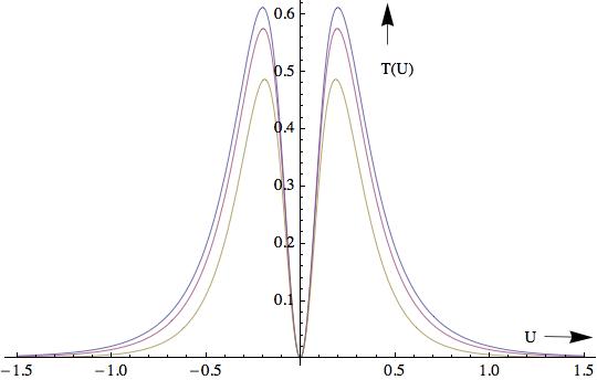
Figure 1: Variation of $T(U)$ as a function $U$ for $m=0,1$ and $2$ respectively. We have set $\ell=1$ and choose $r_{+}=1/2\pi$. The maximum value of $T(U)$ decreases with increasing $m$.

We now turn our attention to the average null energy for the $\mathbb{RP}^{2}$-geon. Here we need to sum the contribution from all the images as described in (3.27), with $(\varphi-\varphi_{n}^{\prime})=(2n+1)\pi$. Since $T(U)$ is positive definite, we need to choose anti-periodic boundary condition for the vector field $A_{\rho}(x)$ in the quotient space in order to violate the ANEC. The average null energy is now given by

$$\langle T\rangle=-\sum_{n=0}^{\infty}t_{n}\ ,$$ (3.36)

where $t_{n}$ is defined as (with $c_{n}\equiv\cosh\left(\nicefrac{{(2n+1)\pi r_{+}}}{{\ell}}\right)$):

$$t_{n}=2\int_{c_{n}}^{\infty}du\sqrt{\left(u-c_{n}\right)}\frac{\left(1+2u+m\ell(u+2)\sqrt{u^{2}-1}+m^{2}\ell^{2}(u^{2}-1)\right)}{\pi\ell(u^{2}-1)^{5/2}\left(u+\sqrt{u^{2}-1}\right)^{m\ell}}\ .$$ (3.37)

The integration can be exactly evaluated for certain specific values of the parameters to express it in terms of elliptic functions. The result is not in particular illuminating. We will instead evaluate it numerically. Without loss of generality we will set the $AdS$ radius $\ell$ to one. The values $t_{n}$ for different choices of $m$ and $r_{+}$ are depicted in Figs. 2 and 3.

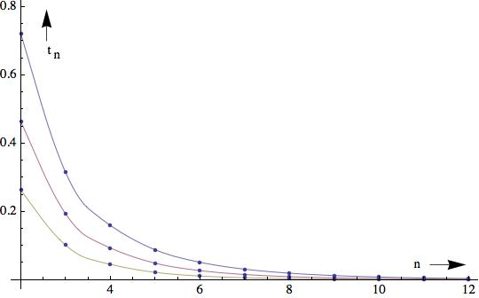
Figure 2: Variation of $t_{n}$ with respect to $n$ for $r_{+}=1/12\pi,1/10\pi$ and $1/8\pi$ respectively. We have set $m=0$ and $\ell=1$. The values of $t_{n}$ for a fixed $n$ decrease with increasing $r_{+}$.

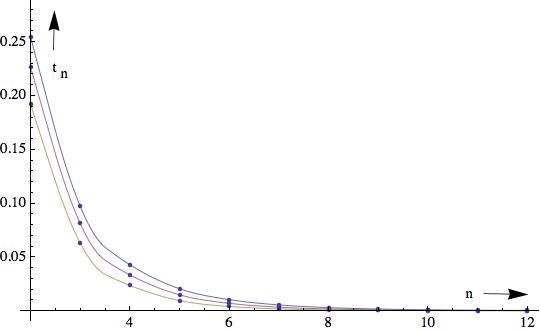
Figure 3: Variation of $t_{n}$ with respect to $n$ for $m=1/2,1$ and $3/2$ respectively. We have set $r_{+}=1/8\pi$ and $\ell=1$. The values of $t_{n}$ for a fixed $n$ decrease with increasing $m$.

From the numerical analysis we can see that the value of $t_{n}$ drops rapidly for large $n$ and the series (3.36) indeed converges quickly. In the following we will prove the convergence analytically. Note that we can express $t_{n}$ as:

$$t_{n}=\frac{2}{\pi\ell}\int_{c_{n}}^{\infty}duf(u)\frac{\sqrt{u-c_{n}}}{u^{2}-1}\ ,$$ (3.38)

with

$$f(u)=\frac{\left(1+2u+m\ell(u+2)\sqrt{u^{2}-1}+m^{2}\ell^{2}(u^{2}-1)\right)}{(u^{2}-1)^{3/2}\left(u+\sqrt{u^{2}-1}\right)^{m\ell}}\ .$$ (3.39)

Now, observe that, for any given $r_{+}>0$, there exists an integer $N$ such that the function $f(u)$ as defined above takes value in the range $0<f(u)<1$ for $u>c_{N}$, for all $m\ell>0$. As a consequence of the above, if we introduce

$$\tilde{t}_{n}=\frac{2}{\pi\ell}\int_{c_{n}}^{\infty}du\frac{\sqrt{u-c_{n}}}{u^{2}-1}\ ,$$ (3.40)

we find $\tilde{t}_{n}>t_{n}$ for all $n>N$. The integration in (3.40) can be evaluated exactly to find

$$\tilde{t}_{n}=\frac{1}{\ell}\big{(}\sqrt{c_{n}+1}-\sqrt{c_{n}-1}\big{)}\ .$$ (3.41)

Substituting $c_{n}=\cosh\left(\nicefrac{{(2n+1)\pi r_{+}}}{{\ell}}\right)$ in the above we find that:

$$\lim_{n\rightarrow\infty}\frac{\tilde{t}_{n+1}}{\tilde{t}_{n}}=e^{-\pi r_{+}/\ell}\ .$$ (3.42)

Thus, the series $\sum_{n=N}^{\infty}\tilde{t}_{n}$ converges for any $r_{+}/\ell>0$. As a consequence, the series $\sum_{n=N}^{\infty}t_{n}$ as well as the one given in (3.36) converges giving rise to a finite value for $\Delta V(\infty)$.

From the numerical analysis we find that, for a fixed value of $r_{+}$ the opening of the wormhole is maximum when the mass of the vector field saturates the BF bound. The size decreases as we increase $m$ and the wormhole closes in the limit $m\rightarrow\infty$. Similarly, for fixed $m$ the opening decreases as we increase the value of $r_{+}$. The size of opening remains finite for finite values of $m$ and $r_{+}$. This is in contrast to the case of scalar fields [14], where the average null energy diverges and one needs to adopt a regularisation process to get a finite size of the opening of the wormhole.

4 Conclusion

In this paper we have discussed the issue of traversability of wormholes in a quotient of the BTZ space-time by certain $\mathbb{Z}_{2}$ symmetry in the presence of massive vector fields. We have obtained the expression for the two-point function of the vector fields in $AdS_{3}$. Using this we have computed the average null energy and found that it becomes negative for appropriate choice of boundary conditions on the vector fields. The back reaction on the geometry then makes the wormholes traversable. It would be interesting to extend our analysis for quotients of $BTZ$ as well as $BTZ\times S^{1}$ geometries by more general discrete symmetries as well as study the effect of rotation on the traversability. It is also worth generalising this to study the traversability of wormholes in the presence of higher spin fields. Similar analysis can be carried out for higher dimensional black holes as well. More generally, recent studies have shown that the Euclidean wormholes play a significant role in giving a new perspective on the information loss paradox. It would be interesting to see whether the issue of traversability in Lorentzian wormholes such as the ones studied in the present work shed any light on this problem.

Acknowledgement

This work is partially supported by the DST project grant EMR/2016/001997.

Appendix A The two-point function

In this appendix we will derive the two-point function involving the field strengths corresponding to the gauge field $A_{\rho}(x)$ in $AdS_{3}$. Consider the Green’s function

$$\langle A_{\rho}(x)A_{\sigma^{\prime}}(x^{\prime})\rangle=\upalpha(\upmu)g_{\rho\sigma^{\prime}}(x,x^{\prime})+\upbeta(\upmu)n_{\rho}(x,x^{\prime})n_{\sigma^{\prime}}(x,x^{\prime})\ .$$ (A.1)

The expressions for $\upalpha(\upmu)$ and $\upbeta(\upmu)$ have been derived in (3.19). For maximally symmetric spaces, the parallel propagator $g_{\mu\nu^{\prime}}(x,x^{\prime})$ along the geodesic joining $x^{\prime}$ to $x^{\prime}$ is unique. It has the following properties:

$$g_{\mu\nu^{\prime}}(x,x^{\prime}) = g_{\mu\nu}(x)\ {\rm for}\ x^{\prime}=x,$$ (A.2)

$$g_{\mu\nu^{\prime}}(x,x^{\prime}) = g_{\nu^{\prime}\mu}(x^{\prime},x)\ ,$$ (A.3)

$$g_{\mu\nu}(x) = g_{\mu\rho^{\prime}}(x,x^{\prime})g_{\nu\sigma^{\prime}}(x,x^{\prime})g^{\rho^{\prime}\sigma^{\prime}}(x^{\prime})\ .$$ (A.4)

We need to evaluate $\langle F_{\eta\delta}(x)F_{\rho^{\prime}\sigma^{\prime}}(x^{\prime})\rangle$. Let us first compute $\langle\nabla_{\eta}A_{\delta}(x)\nabla_{\rho^{\prime}}A_{\sigma^{\prime}}(x^{\prime})\rangle$. In order to do so, we need to know the action of the covariant derivative on bitensors. This has been worked out in general for arbitrary dimensions in [18]. In the following we will list the formulae relevant for our purpose:

$$\nabla_{\rho}n_{\sigma}(x,x^{\prime}) = A(\upmu)\big{(}g_{\rho\sigma}(x)-n_{\rho}(x,x^{\prime})n_{\sigma}(x,x^{\prime})\big{)}\ ,$$ (A.5)

$$\nabla_{\rho}n_{\sigma^{\prime}}(x,x^{\prime}) = C(\upmu)\big{(}g_{\rho\sigma^{\prime}}(x,x^{\prime})+n_{\rho}(x,x^{\prime})n_{\sigma^{\prime}}(x,x^{\prime})\big{)}\ ,$$ (A.6)

$$\nabla_{\rho}g_{\sigma\eta^{\prime}}(x,x^{\prime}) = -\big{(}A(\upmu)+C(\upmu)\big{)}\big{(}g_{\rho\sigma}(x)n_{\eta^{\prime}}(x,x^{\prime})+g_{\rho\eta^{\prime}}(x,x^{\prime})\eta_{\sigma}(x,x^{\prime})\big{)}\ ,$$ (A.7)

and analogous expressions for the derivatives with respect to $\nabla_{\rho^{\prime}}$. The functions $A(\upmu)$ and $C(\upmu)$ are defined as

$$A(\upmu)=\frac{1}{\ell}\coth\left(\nicefrac{{\upmu}}{{\ell}}\right),\ {\rm and}\ C(\upmu)=-\frac{1}{\ell}\rm{cosech}\left(\nicefrac{{\upmu}}{{\ell}}\right)\ .$$ (A.8)

In addition, note that the covariant derivative acts on an arbitrary function $f(\upmu)$ as $\nabla_{\rho}f(\upmu)=f^{\prime}(\upmu)\nabla_{\rho}\upmu=f^{\prime}(\upmu)n_{\rho}(x,x^{\prime})$, where the prime denotes the derivative with respect to the argument.

Using these relations we find,

$$\langle\nabla_{\eta}A_{\delta}(x)\nabla_{\rho^{\prime}}A_{\sigma^{\prime}}(x^{\prime})\rangle = f_{1}(\upmu)g_{\delta\sigma^{\prime}}n_{\eta}n_{\rho^{\prime}}+f_{2}(\upmu)g_{\delta\rho^{\prime}}n_{\eta}n_{\sigma^{\prime}}+f_{3}(\upmu)g_{\eta\rho^{\prime}}n_{\delta}n_{\sigma^{\prime}}+f_{4}(\upmu)g_{\eta\sigma^{\prime}}n_{\delta}n_{\rho^{\prime}}$$ (A.9)

$$+ f_{5}(\upmu)g_{\eta\delta}n_{\rho^{\prime}}n_{\sigma^{\prime}}+f_{6}(\upmu)g_{\rho^{\prime}\sigma^{\prime}}n_{\eta}n_{\delta}+f_{7}(\upmu)g_{\delta\sigma^{\prime}}g_{\eta\rho^{\prime}}+f_{8}(\upmu)g_{\eta\delta}g_{\rho^{\prime}\sigma^{\prime}}$$ (A.10)

$$+ f_{9}(\upmu)g_{\eta\sigma^{\prime}}g_{\delta\rho^{\prime}}+f_{10}(\upmu)n_{\eta}n_{\delta}n_{\rho^{\prime}}n_{\sigma^{\prime}}\ ,$$ (A.11)

in terms of the functions $f_{i}(\upmu)$ which have the following expressions:

$$f_{1}=\alpha^{\prime\prime}+\alpha^{\prime}C,\ f_{2}=C\big{(}\beta^{\prime}-\beta(A-C)\big{)}-\alpha^{\prime}(A+C)$$ (A.12)

$$f_{3}=C\big{(}\beta^{\prime}-\beta(A-C)\big{)}-(A+C)\big{(}\beta C-\alpha(A+C)\big{)}$$ (A.13)

$$f_{4}=C\big{(}\beta C-\alpha(A+C)\big{)}+\frac{d}{d\upmu}\big{(}\beta C-\alpha(A+C)\big{)}$$ (A.14)

$$f_{5}=\frac{d}{d\upmu}\big{(}\beta A-\alpha(A+C)\big{)}-A\big{(}\beta A-\alpha(A+C)\big{)}$$ (A.15)

$$f_{6}=A\big{(}\beta^{\prime}-\beta(A-C)\big{)}-(A+C)\big{(}\alpha^{\prime}+\beta C-\alpha(A+C)\big{)}$$ (A.16)

$$f_{7}=\alpha^{\prime}C,f_{8}=A\big{(}\beta A-\alpha(A+C)\big{)},f_{9}=C\big{(}\beta C-\alpha(A+C)\big{)}$$ (A.17)

$$f_{10}=(2C-A)\big{(}\beta^{\prime}-\beta(A-C)\big{)}+\frac{d}{d\upmu}\big{(}\beta^{\prime}-\beta(A-C)\big{)}\ .$$ (A.18)

The two-point function involving the field strengths is now given by

$$\langle F_{\eta\delta}(x)F_{\rho^{\prime}\sigma^{\prime}}(x^{\prime})\rangle = (f_{1}-f_{2}+f_{3}-f_{4})\big{(}g_{\delta\sigma^{\prime}}n_{\eta}n_{\rho^{\prime}}-g_{\eta\sigma^{\prime}}n_{\delta}n_{\rho^{\prime}}+g_{\eta\rho^{\prime}}n_{\delta}n_{\sigma^{\prime}}-g_{\delta\rho^{\prime}}n_{\eta}n_{\sigma^{\prime}}\big{)}$$ (A.19)

$$+ 2(f_{9}-f_{7})\big{(}g_{\eta\sigma^{\prime}}g_{\delta\rho^{\prime}}-g_{\delta\sigma^{\prime}}g_{\eta\rho^{\prime}}\big{)}\ .$$ (A.20)

Substituting the values of $f_{i}(\upmu),A(\upmu)$ and $C(\upmu)$ in the above we obtain (3.20).

Appendix B The geodesic distance

Here we will derive the expression for the geodesic distance in $AdS_{3}$ as well as compute the unit vectors $n_{\mu}(x,x^{\prime})$ and $n_{\mu^{\prime}}(x,x^{\prime})$. To find the geodesic distance, we consider the embedding of $AdS_{3}$ in $(2,2)$ Minkowski space with co-ordinates $Y^{a}$. The geodesic distance $\upmu(x,x^{\prime})$ is then given by

$$\cosh\left(\nicefrac{{\upmu(x,x^{\prime})}}{{\ell}}\right)=-\frac{1}{\ell^{2}}\eta_{ab}Y^{a}(x)Y^{b}(x^{\prime})\ .$$ (B.1)

We use the Kruskal-like coordinates $x^{\mu}=(U,V,\varphi)$ such that

$$Y^{0} = \ell\frac{U+V}{1+UV}\ ,\ \ Y^{1}=\ell\frac{1-UV}{1+UV}\cosh\left(\nicefrac{{r_{+}\varphi}}{{\ell}}\right)\ ,$$ (B.2)

$$Y^{2} = \ell\frac{U-V}{1+UV}\ ,\ \ Y^{3}=\ell\frac{1-UV}{1+UV}\sinh\left(\nicefrac{{r_{+}\varphi}}{{\ell}}\right)\ .$$ (B.3)

In terms of these coordinates, the geodesic distance $\upmu(x,x^{\prime})$ between points $x$ and $x^{\prime}$ is

$$\cosh\left(\nicefrac{{\upmu}}{{\ell}}\right)=\frac{\Big{(}2\left(UV^{\prime}+VU^{\prime}\right)+\left(1-UV\right)\left(1-U^{\prime}V^{\prime}\right)\cosh\left(\nicefrac{{r_{+}(\varphi-\varphi^{\prime})}}{{\ell}}\right)\Big{)}}{\left(1+UV\right)\left(1+U^{\prime}V^{\prime}\right)}\ .$$ (B.4)

It is now straightforward to compute the components of the unit tangents $n_{\rho}(x,x^{\prime})$ and $n_{\rho^{\prime}}(x,x^{\prime})$. We find

$$n_{U}(x,x^{\prime}) = \frac{2\ell}{\sinh\left(\nicefrac{{\upmu}}{{\ell}}\right)}\frac{\Big{(}V^{\prime}-V^{2}U^{\prime}-\left(1-U^{\prime}V^{\prime}\right)V\cosh\left(\nicefrac{{r_{+}(\varphi-\varphi^{\prime})}}{{\ell}}\right)\Big{)}}{\left(1+UV\right)^{2}\left(1+U^{\prime}V^{\prime}\right)}$$ (B.5)

$$n_{V}(x,x^{\prime}) = \frac{2\ell}{\sinh\left(\nicefrac{{\upmu}}{{\ell}}\right)}\frac{\Big{(}U^{\prime}-U^{2}V^{\prime}-(1-U^{\prime}V^{\prime})U\cosh\left(\nicefrac{{r_{+}(\varphi-\varphi^{\prime})}}{{\ell}}\right)\Big{)}}{\left(1+UV\right)^{2}\left(1+U^{\prime}V^{\prime}\right)}$$ (B.6)

$$n_{\varphi}(x,x^{\prime}) = \frac{r_{+}}{\sinh\left(\nicefrac{{\upmu}}{{\ell}}\right)}\frac{\Big{(}\left(1-UV\right)\left(1-U^{\prime}V^{\prime}\right)\sinh\left(\nicefrac{{r_{+}(\varphi-\varphi^{\prime})}}{{\ell}}\right)\Big{)}}{\left(1+UV\right)\left(1+U^{\prime}V^{\prime}\right)}\ .$$ (B.7)

Likewise, components of the unit tangent $n_{\rho^{\prime}}(x,x^{\prime})=\nabla_{\rho^{\prime}}\upmu(x,x^{\prime})$ at $x^{\prime}$ are

$$n_{U^{\prime}}(x,x^{\prime}) = \frac{2\ell}{\sinh\left(\nicefrac{{\upmu}}{{\ell}}\right)}\frac{\Big{(}V-UV^{\prime 2}-\left(1-UV\right)V^{\prime}\cosh\left(\nicefrac{{r_{+}(\varphi-\varphi^{\prime})}}{{\ell}}\right)\Big{)}}{\left(1+UV\right)\left(1+U^{\prime}V^{\prime}\right)^{2}}$$ (B.8)

$$n_{V^{\prime}}(x,x^{\prime}) = \frac{2\ell}{\sinh\left(\nicefrac{{\upmu}}{{\ell}}\right)}\frac{\Big{(}U-VU^{\prime 2}-(1-UV)U^{\prime}\cosh\left(\nicefrac{{r_{+}(\varphi-\varphi^{\prime})}}{{\ell}}\right)\Big{)}}{\left(1+UV\right)\left(1+U^{\prime}V^{\prime}\right)^{2}}$$ (B.9)

$$n_{\varphi^{\prime}}(x,x^{\prime}) = -\frac{r_{+}}{\sinh\left(\nicefrac{{\upmu}}{{\ell}}\right)}\frac{\Big{(}\left(1-UV\right)\left(1-U^{\prime}V^{\prime}\right)\sinh\left(\nicefrac{{r_{+}(\varphi-\varphi^{\prime})}}{{\ell}}\right)\Big{)}}{\left(1+UV\right)\left(1+U^{\prime}V^{\prime}\right)}\ .$$ (B.10)

Setting $x^{\prime}=Jx$, we find

$$n_{U}(x,Jx) = \frac{2\ell\left(U-V^{3}-V(1-UV)\cosh\left(\nicefrac{{k\pi r_{+}}}{{\ell}}\right)\right)}{\sinh\left(\nicefrac{{\upmu}}{{\ell}}\right)\left(1+UV\right)^{3}}$$ (B.11)

$$n_{V}(x,Jx) = \frac{2\ell\left(V-U^{3}-U(1-UV)\cosh\left(\nicefrac{{k\pi r_{+}}}{{\ell}}\right)\right)}{\sinh\left(\nicefrac{{\upmu}}{{\ell}}\right)\left(1+UV\right)^{3}}$$ (B.12)

$$n_{\varphi}(x,Jx) = -\frac{r_{+}\left(1-UV\right)^{2}\sinh\left(\nicefrac{{k\pi r_{+}}}{{\ell}}\right)}{\sinh\left(\nicefrac{{\upmu}}{{\ell}}\right)\left(1+UV\right)^{2}}\ ,$$ (B.13)

and

$$n_{U^{\prime}}(x,Jx) = \frac{2\ell\left(V-U^{3}-U(1-UV)\cosh\left(\nicefrac{{k\pi r_{+}}}{{\ell}}\right)\right)}{\sinh\left(\nicefrac{{\upmu}}{{\ell}}\right)\left(1+UV\right)^{3}}$$ (B.14)

$$n_{V^{\prime}}(x,Jx) = \frac{2\ell\left(U-V^{3}-V(1-UV)\cosh\left(\nicefrac{{k\pi r_{+}}}{{\ell}}\right)\right)}{\sinh\left(\nicefrac{{\upmu}}{{\ell}}\right)\left(1+UV\right)^{3}}$$ (B.15)

$$n_{\varphi^{\prime}}(x,Jx) = \frac{r_{+}\left(1-UV\right)^{2}\sinh\left(\nicefrac{{k\pi r_{+}}}{{\ell}}\right)}{\sinh\left(\nicefrac{{\upmu}}{{\ell}}\right)\left(1+UV\right)^{2}}\ .$$ (B.16)

Appendix C The parallel propagator

In this appendix we will analyse the behaviour of the parallel propagator on the $V=0$ surface. The parallel propagator $g_{\mu\nu^{\prime}}(x,x^{\prime})$ is a linear map which parallel transports vectors $V^{\rho^{\prime}}(x^{\prime})$ at the point $x^{\prime}$ to $V^{\rho}(x)$ at the point $x$:

$$g_{\mu\nu^{\prime}}(x,x^{\prime})V^{\nu^{\prime}}(x^{\prime})=V_{\mu}(x)\ .$$ (C.1)

The equation of motion for the parallel propagator can be obtained from the equation for parallel transport of a vector and is given by:

$$\frac{d}{d\lambda}{g^{\mu}}_{\nu^{\prime}}(x,x^{\prime})+\Gamma^{\mu}_{\nu\rho}\frac{dx^{\nu}}{d\lambda}{g^{\rho}}_{\nu^{\prime}}(x,x^{\prime})=0\ .$$ (C.2)

It depends on the path $x^{\mu}(\lambda)$ and has the following formal solution in terms of the path-ordered exponential [19]:

$${g^{\mu}}_{\nu^{\prime}}(x,x^{\prime})={\cal P}\exp\left(-\int_{\lambda^{\prime}}^{\lambda}\Gamma^{\mu}_{\sigma\nu}\frac{dx^{\sigma}}{d\lambda}d\lambda\right)\ .$$ (C.3)

In the following we will analyse (C.2) for $AdS_{3}$ in detail. The non-vanishing components of the affine connection are listed as:

$$\Gamma^{U}_{UU}=-\frac{2V}{1+UV}\ ,\ \Gamma^{U}_{\varphi\varphi}=-\frac{r_{+}^{2}U(1-UV)}{\ell^{2}(1+UV)}\ ,$$ (C.4)

$$\Gamma^{V}_{VV}=-\frac{2U}{1+UV}\ ,\ \Gamma^{V}_{\varphi\varphi}=-\frac{r_{+}^{2}V(1-UV)}{\ell^{2}(1+UV)}\ ,$$ (C.5)

$$\Gamma^{\varphi}_{\varphi U}=-\frac{2V}{1-U^{2}V^{2}}\ ,\ \Gamma^{\varphi}_{\varphi V}=-\frac{2U}{1-U^{2}V^{2}}\ .$$ (C.6)

The equation of motion (C.2) for the parallel propagator now becomes

$$\frac{d}{d\lambda}{g^{U}}_{U^{\prime}}-\frac{2V}{1+UV}\frac{dU}{d\lambda}{g^{U}}_{U^{\prime}}-\frac{r_{+}^{2}U(1-UV)}{\ell^{2}(1+UV)}\frac{d\varphi}{d\lambda}{g^{\varphi}}_{U^{\prime}}=0,$$ (C.7)

$$\frac{d}{d\lambda}{g^{U}}_{V^{\prime}}-\frac{2V}{1+UV}\frac{dU}{d\lambda}{g^{U}}_{V^{\prime}}-\frac{r_{+}^{2}U(1-UV)}{\ell^{2}(1+UV)}\frac{d\varphi}{d\lambda}{g^{\varphi}}_{V^{\prime}}=0,$$ (C.8)

$$\frac{d}{d\lambda}{g^{U}}_{\varphi^{\prime}}-\frac{2V}{1+UV}\frac{dU}{d\lambda}{g^{U}}_{\varphi^{\prime}}-\frac{r_{+}^{2}U(1-UV)}{\ell^{2}(1+UV)}\frac{d\varphi}{d\lambda}{g^{\varphi}}_{\varphi^{\prime}}=0,$$ (C.9)

$$\frac{d}{d\lambda}{g^{V}}_{U^{\prime}}-\frac{2U}{1+UV}\frac{dV}{d\lambda}{g^{V}}_{U^{\prime}}-\frac{r_{+}^{2}V(1-UV)}{\ell^{2}(1+UV)}\frac{d\varphi}{d\lambda}{g^{\varphi}}_{U^{\prime}}=0,$$ (C.10)

$$\frac{d}{d\lambda}{g^{V}}_{V^{\prime}}-\frac{2U}{1+UV}\frac{dV}{d\lambda}{g^{V}}_{V^{\prime}}-\frac{r_{+}^{2}V(1-UV)}{\ell^{2}(1+UV)}\frac{d\varphi}{d\lambda}{g^{\varphi}}_{V^{\prime}}=0,$$ (C.11)

$$\frac{d}{d\lambda}{g^{V}}_{\varphi^{\prime}}-\frac{2U}{1+UV}\frac{dV}{d\lambda}{g^{V}}_{\varphi^{\prime}}-\frac{r_{+}^{2}V(1-UV)}{\ell^{2}(1+UV)}\frac{d\varphi}{d\lambda}{g^{\varphi}}_{\varphi^{\prime}}=0,$$ (C.12)

$$\frac{d}{d\lambda}{g^{\varphi}}_{U^{\prime}}-\frac{2}{1-U^{2}V^{2}}\left(V\frac{d\varphi}{d\lambda}{g^{U}}_{U^{\prime}}+U\frac{d\varphi}{d\lambda}{g^{V}}_{U^{\prime}}+\frac{d(UV)}{d\lambda}{g^{\varphi}}_{U^{\prime}}\right)=0$$ (C.13)

$$\frac{d}{d\lambda}{g^{\varphi}}_{V^{\prime}}-\frac{2}{1-U^{2}V^{2}}\left(V\frac{d\varphi}{d\lambda}{g^{U}}_{V^{\prime}}+U\frac{d\varphi}{d\lambda}{g^{V}}_{V^{\prime}}+\frac{d(UV)}{d\lambda}{g^{\varphi}}_{V^{\prime}}\right)=0$$ (C.14)

$$\frac{d}{d\lambda}{g^{\varphi}}_{\varphi^{\prime}}-\frac{2}{1-U^{2}V^{2}}\left(V\frac{d\varphi}{d\lambda}{g^{U}}_{\varphi^{\prime}}+U\frac{d\varphi}{d\lambda}{g^{V}}_{\varphi^{\prime}}+\frac{d(UV)}{d\lambda}{g^{\varphi}}_{\varphi^{\prime}}\right)=0$$ (C.15)

The above equations need to be analysed along the geodesic:

$$\frac{d^{2}x^{\rho}}{d\lambda^{2}}+\Gamma^{\rho}_{\eta\sigma}\frac{dx^{\eta}}{d\lambda}\frac{dx^{\sigma}}{d\lambda}=0.$$ (C.16)

For the present case this becomes

$$\frac{d^{2}U}{d\lambda^{2}}-\frac{2V}{1+UV}\left(\frac{dU}{d\lambda}\right)^{2}-\frac{r_{+}^{2}U(1-UV)}{\ell^{2}(1+UV)}\left(\frac{d\varphi}{d\lambda}\right)^{2} = 0$$ (C.17)

$$\frac{d^{2}V}{d\lambda^{2}}-\frac{2U}{1+UV}\left(\frac{dV}{d\lambda}\right)^{2}-\frac{r_{+}^{2}V(1-UV)}{\ell^{2}(1+UV)}\left(\frac{d\varphi}{d\lambda}\right)^{2} = 0$$ (C.18)

$$\frac{d^{2}\varphi}{d\lambda^{2}}-\frac{4}{1-U^{2}V^{2}}\frac{d(UV)}{d\lambda}\frac{d\varphi}{d\lambda} = 0$$ (C.19)

We will now choose $U$ to be the affine parameter. Setting $V=0$ in the geodesic equation, we can easily see that $\frac{d\varphi}{dU}=0$. Using this in (C.7), we find that the term $\Gamma^{\mu}_{\nu\rho}\frac{dx^{\nu}}{d\lambda}{g^{\rho}}_{\nu^{\prime}}(x,x^{\prime})$ vanishes identically and hence ${g^{\rho}}_{\sigma^{\prime}}(x,x^{\prime})$ is independent of $U$ on the $V=0$ surface.

References

- [1] M. S. Morris and K. S. Thorne, Am. J. Phys. 56, 395-412 (1988) doi:10.1119/1.15620
- [2] D. Hochberg and M. Visser, Phys. Rev. D 58, 044021 (1998) doi:10.1103/PhysRevD.58.044021 [arXiv:gr-qc/9802046 [gr-qc]].
- [3] M. S. Morris, K. S. Thorne and U. Yurtsever, Phys. Rev. Lett. 61, 1446-1449 (1988) doi:10.1103/PhysRevLett.61.1446
- [4] M. Visser, S. Kar and N. Dadhich, Phys. Rev. Lett. 90, 201102 (2003) doi:10.1103/PhysRevLett.90.201102 [arXiv:gr-qc/0301003 [gr-qc]].
- [5] N. Graham and K. D. Olum, Phys. Rev. D 76, 064001 (2007) doi:10.1103/PhysRevD.76.064001 [arXiv:0705.3193 [gr-qc]].
- [6] A. C. Wall, Phys. Rev. D 81, 024038 (2010) doi:10.1103/PhysRevD.81.024038 [arXiv:0910.5751 [gr-qc]].
- [7] W. R. Kelly and A. C. Wall, Phys. Rev. D 90, no.10, 106003 (2014) doi:10.1103/PhysRevD.90.106003 [arXiv:1408.3566 [gr-qc]].
- [8] J. L. Friedman, K. Schleich and D. M. Witt, Phys. Rev. Lett. 71, 1486-1489 (1993) doi:10.1103/PhysRevLett.71.1486 [arXiv:gr-qc/9305017 [gr-qc]].
- [9] G. J. Galloway, K. Schleich, D. M. Witt and E. Woolgar, Phys. Rev. D 60, 104039 (1999) doi:10.1103/PhysRevD.60.104039 [arXiv:gr-qc/9902061 [gr-qc]].
- [10] P. Gao, D. L. Jafferis and A. C. Wall, JHEP 12, 151 (2017) doi:10.1007/JHEP12(2017)151 [arXiv:1608.05687 [hep-th]].
- [11] E. Caceres, A. S. Misobuchi and M. L. Xiao, JHEP 12, 005 (2018) doi:10.1007/JHEP12(2018)005 [arXiv:1807.07239 [hep-th]].
- [12] J. Maldacena and X. L. Qi, [arXiv:1804.00491 [hep-th]].
- [13] J. Maldacena, A. Milekhin and F. Popov, [arXiv:1807.04726 [hep-th]].
- [14] Z. Fu, B. Grado-White and D. Marolf, Class. Quant. Grav. 36, no.4, 045006 (2019) doi:10.1088/1361-6382/aafcea [arXiv:1807.07917 [hep-th]].
- [15] D. Marolf and S. McBride, JHEP 11, 037 (2019) doi:10.1007/JHEP11(2019)037 [arXiv:1908.03998 [hep-th]].
- [16] J. M. Maldacena, JHEP 04, 021 (2003) doi:10.1088/1126-6708/2003/04/021 [arXiv:hep-th/0106112 [hep-th]].
- [17] J. Louko and D. Marolf, Phys. Rev. D 59, 066002 (1999) doi:10.1103/PhysRevD.59.066002 [arXiv:hep-th/9808081 [hep-th]].
- [18] B. Allen and T. Jacobson, Commun. Math. Phys. 103, 669 (1986) doi:10.1007/BF01211169
- [19] S. M. Carroll, [arXiv:gr-qc/9712019 [gr-qc]].