High energy QCD: multiplicity dependence of quarkonia production

Abstract

In this paper we propose an approach which demonstrates the dependence of quarkonia production on the multiplicity of the accompanying hadrons. Our approach is based on the three gluon fusion mechanism, without assuming the multiplicity dependence of the saturation scale. We show, that we describe the experimental data, which has a dependence that is much steeper than the multiplicity of the hadrons.

I Introduction

The goal of this paper is to study the multiplicity dependence of quarkonia (mainly $J/\Psi$) production in the framework of high energy QCD (see Ref.KOLEB for a general review). Effective QCD at high energies currently exists in two different formulations: the CGC/saturation approach MV ; MUCD ; B ; K ; JIMWLK ; GIJMV , and the BFKL Pomeron calculus BFKL ; LI ; GLR ; GLR1 ; MUQI ; MUPA ; BART ; BRN ; KOLE ; LELU1 ; LELU2 ; LMP ; AKLL ; AKLL1 ; LEPP . In this paper we restrict ourself to the BFKL Pomeron calculus, which has a more direct correspondence with the parton approach, and which provides an approximation for estimates of hadron-hadron collisions, that at present are out of the reach for the CGC approach.

Fortunately, in Ref.AKLL1 it was shown, that these two approaches are equivalent for the description of the scattering amplitude in the rapidity range :

$$Y\,\leq\,\frac{2}{\Delta_{\mbox{\tiny BFKL}}}\,\ln\left(\frac{1}{\Delta^{2}_{\mbox{\tiny BFKL}}}\right)$$ (1)

where $\Delta_{\mbox{\tiny BFKL}}$ denotes the intercept of the BFKL Pomeron. In this paper it is also shown, that for Eq. (1) we can use the Mueller, Patel, Salam and Iancu approximation(MPSI) MPSI for hadron-hadron scattering at high energies.

The recent experiments by ALICEALICE0 ; ALICE1 ; ALICE01 ; ALICE2 ; ALICE3 and STARSTAR1 ; STAR2 , show that the cross sections for $J/\Psi$ production depends strongly on the multiplicity of accompanying hadrons. These data have stimulated theoretical discussions on the origin of such dependence (see Refs.KPPRS ; FEPA ; MTVW ; LESI ; LSS ). In this paper, we develop an approach to this problem based on two ingredients. First, we assume ,that the production of quarkonia stems from triple gluon fusionKMRS ; MOSA ; LESI (see Fig. 1). For the interaction with nuclei this mechanism is dominant KHTU ; KLNT ; DKLMT ; KLTPSI ; KMV ; and it has been demonstrated in Ref.LESI , that this mechanism gives a substantial contribution in hadron-hadron collisions.

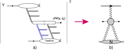
Figure 1: Fig. 1-a: The three gluon fusion mechanism of $J/\Psi$ production.Fig. 1-b: the Mueller diagramMUDIA for $J/\Psi$ production, which illustrates the inter-relation between three gluon fusion and the triple BFKL Pomeron interaction. The wavy lines describe the BFKL Pomerons, while the helical curves represent gluons.

Second, we showed in Refs.GOLEMULT ; KHLE , that in spite of the fact that in different kinematic regions, the QCD cascade leads to a different energy and dipole size dependence of the mean multiplicity, the multiplicity distribution has a general form:

$$\frac{\sigma_{n}}{\sigma_{\rm in}}\,\,=\,\,\frac{1}{N}\,\left(\frac{N\,-\,1}{N}\right)^{n-1}\,$$ (2)

where N denotes the average number of partons.

The paper is organized as follows: In the next section we describe our approach to hadron-hadron collisions. In section III we discuss quarkonia production in simplified Reggeon Field Theory, defined in zero transverse dimensions. In section IV we generalize the result in this toy-model approach to high energy QCD, and compare our estimates with the experimental data . We summarize our results in the Conclusions.

II Hadron-hadron interaction in MPSI approach

This section does not contain new results, and we include it in the paper for completeness of presentation, as well as a kind of an introduction to the notation, and the main ideas.

II.1 QCD parton cascade

We start with the equation for the QCD parton cascade which can be written in the following form.KOLEB ; MUCD ; LELU1 ; LELU2 :

$$\frac{\partial\,P_{n}\left(Y,\boldsymbol{r},\boldsymbol{b};\,\boldsymbol{r}_{1},\boldsymbol{b}_{1},\,\boldsymbol{r}_{2},\boldsymbol{b}_{2}\dots\boldsymbol{r}_{i},\boldsymbol{b}_{i},\dots\boldsymbol{r}_{n},\boldsymbol{b}_{n}\right)}{\partial\,Y}\,=\,-\,\sum^{n}_{i=1}\,\omega_{G}(r_{i})\,P_{n}\left(Y,\boldsymbol{r},\boldsymbol{b};\,\boldsymbol{r}_{1},\boldsymbol{b}_{1},\,\boldsymbol{r}_{2},\boldsymbol{b}_{2}\dots\boldsymbol{r}_{i},\boldsymbol{b}_{i},\dots\boldsymbol{r}_{n},\boldsymbol{b}_{n}\right)$$ (3)

$$~{}~{}~{}~{}~{}~{}~{}~{}~{}~{}~{}~{}~{}~{}~{}~{}~{}~{}~{}~{}~{}~{}~{}~{}~{}~{}~{}~{}~{}~{}~{}~{}~{}~{}~{}~{}~{}~{}~{}~{}~{}~{}~{}~{}~{}+\,\,\bar{\alpha}_{S}\,\sum^{n-1}_{i=1}\,\frac{(\boldsymbol{r}_{i}\,+\,\boldsymbol{r}_{n})^{2}}{(2\,\pi)\,r^{2}_{i}\,r^{2}_{n}}\,P_{n-1}\left(Y,\boldsymbol{r},\boldsymbol{b};\,\boldsymbol{r}_{1},\boldsymbol{b}_{1},\dots(\boldsymbol{r}_{i}\,+\,\boldsymbol{r}_{n}),\boldsymbol{b}_{in},\dots\boldsymbol{r}_{n-1},\boldsymbol{b}_{n}\right)$$

where $P_{n}\left(Y;\{r_{i},b_{i}\}\right)$ denotes the probability to have $n$-dipoles of size $r_{i}$, at impact parameter $b_{i}$, and at rapidity $Y$ . $\boldsymbol{b}_{in}$ in Eq. (3) is given by $\boldsymbol{b}_{in}\,=\,\boldsymbol{b}_{i}\,+\,\frac{1}{2}\boldsymbol{r}_{i}\,=\,\boldsymbol{b}_{n}\,-\,\frac{1}{2}\boldsymbol{r}_{i}$.

Eq. (3) is a typical cascade equation in which the first term describes the depletion of the probability of $n$, due to one dipole decaying into two dipoles of arbitrary sizes, while the second term describes, the growth due to the splitting of ($n-1$) dipoles into $n$ dipoles.

The initial condition for the DIS scattering is

$$P_{1}\left(Y=0,\boldsymbol{r},\boldsymbol{b};\boldsymbol{r}_{1},\boldsymbol{b}_{1}\right)\,\,=\,\,\,\delta^{(2)}\left(\boldsymbol{r}\,-\,\boldsymbol{r}_{1}\right)\,\delta^{(2)}\left(\boldsymbol{b}\,-\,\boldsymbol{b}_{1}\right);~{}~{}~{}~{}~{}~{}~{}P_{n>1}\left(Y=0;\{r_{i}\}\right)\,=\,0$$ (4)

which corresponds to the fact that we are discussing a dipole of definite size which develops the parton cascade.

Since $P_{n}\left(Y;\{r_{i}\}\right)$ is the probability to find dipoles $\{r_{i}\}$, we have the following sum rule

$$\sum_{n=1}^{\infty}\,\int\prod^{n}_{i=1}d^{2}r_{i}\,d^{2}b_{i}\,P_{n}\left(Y;\{\boldsymbol{r}_{i}\,\boldsymbol{b}_{i}\}\right)\,\,=\,\,1,$$ (5)

i.e. the sum of all probabilities is equal to 1.

This QCD cascade leads to the Balitsky-Kovchegov (BK) equation B ; K ; KOLEB for the amplitude, and gives the theoretical description of DIS. To see this we introduce the generating functionalMUCD

$$Z\left(Y,\boldsymbol{r},\boldsymbol{b};[u_{i}]\right)\,\,=\,\,\sum^{\infty}_{n=1}\int P_{n}\left(Y,\boldsymbol{r},\boldsymbol{b};\{\boldsymbol{r}_{i}\,\boldsymbol{b}_{i}\}\right)\prod^{n}_{i=1}u\left(\boldsymbol{r}_{i}\,\boldsymbol{b}_{i}\right)\,d^{2}r_{i}\,d^{2}b_{i}$$ (6)

where $u\left(\boldsymbol{r}_{i}\,\boldsymbol{b}_{i}\right)\equiv\,=u_{i}$ is an arbitrary function. The initial conditions of Eq. (4) and the sum rules of Eq. (5) require the following form for the functional $Z$:

$$Z\left(Y=0,\boldsymbol{r},\boldsymbol{b};[u_{i}]\right) \,\,=\,\, u\left(\boldsymbol{r},\boldsymbol{b}\right);$$ (7a)

$$Z\left(Y,r,[u_{i}=1]\right) = 1;$$ (7b)

Multiplying both terms of Eq. (3) by $\prod^{n}_{i=1}u\left(\boldsymbol{r}_{i}\,\boldsymbol{b}_{i}\right)$ and integrating over $r_{i}$ and $b_{i}$, we obtain the following linear functional equationLELU2 ;

$$\frac{\partial Z\left(Y,\boldsymbol{r},\boldsymbol{b};[u_{i}]\right)}{\partial\,Y}=\int d^{2}r^{\prime}\,K\left(\boldsymbol{r}^{\prime},\boldsymbol{r}-\boldsymbol{r^{\prime}}|\boldsymbol{r}\right)\Bigg{(}-u\left(r,b\right)\,\,+\,\,u\left(\boldsymbol{r}^{\prime},\boldsymbol{b}+\frac{1}{2}(\boldsymbol{r}-\boldsymbol{r}^{\prime})\right)\,u\left(\boldsymbol{r}-\boldsymbol{r}^{\prime},\boldsymbol{b}-\frac{1}{2}\boldsymbol{r}^{\prime}\right)\Bigg{)}\frac{\delta\,Z}{\delta\,u\left(r,b\right)};$$ (8a)

$$K\left(\boldsymbol{r}^{\prime},\boldsymbol{r}-\boldsymbol{r^{\prime}}|\boldsymbol{r}\right)\,=\frac{\bar{\alpha}_{S}}{2\,\pi}\frac{r^{2}}{r^{\prime 2}\,(\boldsymbol{r}-\boldsymbol{r}^{\prime})^{2}};\,~{}~{}~{}~{}~{}\omega_{G}\left(r\right)\,\,=\,\,\int d^{2}r^{\prime}K\left(\boldsymbol{r}^{\prime},\boldsymbol{r}-\boldsymbol{r^{\prime}}|\boldsymbol{r}\right);$$ (8b)

Searching for a solution of the form $Z\left([u(r_{i},b_{i},Y)]\right)$ for the initial conditions of Eq. (7a), Eq. (8a) can be re-written as the non-linear equation MUCD :

$$\frac{\partial Z\left(Y,\boldsymbol{r},\boldsymbol{b};[u_{i}]\right)}{\partial\,Y}\,=\,\int d^{2}r^{\prime}K\left(\boldsymbol{r}^{\prime},\boldsymbol{r}-\boldsymbol{r^{\prime}}|\boldsymbol{r}\right)\Bigg{\{}Z\left(r^{\prime},\boldsymbol{b}+\frac{1}{2}(\boldsymbol{r}-\boldsymbol{r}^{\prime});[u_{i}]\right)\,Z\left(\boldsymbol{r}-\boldsymbol{r^{\prime}},\boldsymbol{b}-\frac{1}{2}\boldsymbol{r}^{\prime};[u_{i}]\right)\,\,-\,\,Z\left(Y,\boldsymbol{r},\boldsymbol{b};[u_{i}]\right)\Bigg{\}}$$ (9)

Therefore, the QCD parton cascade of Eq. (3) takes into account non-linear evolution. Generally speaking the scattering amplitude can be written in the formK ; LELU2 :

$$N(Y,\,r,\,b)\,=\,-\,\,\sum^{\infty}_{n=1}\,(-1)^{n}\,\rho^{p}_{n}(r_{1},\,b_{1},\,\ldots\,r_{n},\,b_{n}\,;\,Y\,-\,Y_{0})\,\,\prod^{n}_{i=1}\,N(Y_{0},\,r_{i},\,b_{i})\,\,d^{2}\,r_{i}\,\,d^{2}\,b_{i}\,.$$ (10)

where $N(Y_{0},\,r_{i},\,b_{i})$ is the amplitude of the interaction of dipole $r_{i}$ with the target at low energy $Y=Y_{0}$, and the $n$-dipole densities in the projectile $\rho^{p}_{n}(r_{1},b_{1},\ldots\,,r_{n},b_{n})$ are defined as follows:

$$\rho^{p}_{n}(r_{1},b_{1}\,\ldots\,,r_{n},b_{n};Y\,-\,Y_{0})\,=\,\frac{1}{n!}\,\prod^{n}_{i=1}\,\frac{\delta}{\delta u_{i}}\,Z\left(Y\,-\,Y_{0};\,[u]\right)|_{u=1}$$ (11)

For $\rho_{n}$ we obtainLELU2 :

$$\frac{\partial\,\rho^{p}_{n}(r_{1},b_{1}\,\ldots\,,r_{n},b_{n})}{\bar{\alpha}_{s}\,\partial\,Y}\,\, = \,\ -\,\sum_{i=1}^{n}\,\,\omega(r_{i})\,\,\rho^{p}_{n}(r_{1},b_{1}\,\ldots\,,r_{n},b_{n})\,\,+\,\,2\,\sum_{i=1}^{n}\,\int\,\frac{d^{2}\,r^{\prime}}{2\,\pi}\,\frac{r^{\prime 2}}{r^{2}_{i}\,(\boldsymbol{r}_{i}\,-\,\boldsymbol{r}^{\prime})^{2}}\,\rho^{p}_{n}(\ldots\,r^{\prime},b_{i}-r^{\prime}/2\dots)$$ (12)

$$\,+\,\sum_{i=1}^{n-1}\,\frac{(\boldsymbol{r}_{i}+\boldsymbol{r}_{n})^{2}}{(2\,\pi)\,r^{2}_{i}\,r^{2}_{n}}\,\rho^{p}_{n-1}(\ldots\,(\boldsymbol{r}_{i}\,+\,\boldsymbol{r}_{n}),b_{in}\dots).$$

For $\rho_{1}$ we have the linear BFKL equationBFKL :

$$\frac{\partial\,\rho^{p}_{1}(Y;r_{1},b)}{\bar{\alpha}_{S}\,\partial\,Y}\,\,=\,\,-\,\,\omega_{G}\left(r_{1}\right)\rho^{p}_{1}(Y;r_{1},b)\,\,+\,2\,\int\,\frac{d^{2}\,r^{\prime}}{2\,\pi}\,\frac{r^{\prime 2}}{r^{2}_{1}\,(\boldsymbol{r}_{1}\,-\,\boldsymbol{r}^{\prime})^{2}}\,\bar{\rho}^{p}_{1}\left(Y,r^{\prime},b\right)$$ (13)

However, to obtain the BK equation for the scattering amplitude we need to use Eq. (10), in which we introduce the amplitude of interaction of the dipole with the target at low energies. Using Eq. (8a),Eq. (10) and Eq. (11) , we can obtain the non-linear BK equation from Eq. (9) in the following formK

$$\frac{\partial}{\partial Y}N\left(\boldsymbol{r},\boldsymbol{b},Y\right) = \int d^{2}r^{\prime}\,K\left(\boldsymbol{r}^{\prime},\boldsymbol{r}-\boldsymbol{r}^{\prime}|\boldsymbol{r}\right)\Bigg{\{}N\left(\boldsymbol{r}^{\prime},\boldsymbol{b}-\frac{1}{2}\left(\boldsymbol{r}-\boldsymbol{r}^{\prime}\right),Y\right)+N\left(\boldsymbol{r}-\boldsymbol{r}^{\prime},\boldsymbol{b}-\frac{1}{2}\boldsymbol{r}^{\prime},Y\right)\,\,-\,\,N\left(\boldsymbol{r},\boldsymbol{b},Y\right)$$ (14)

$$~{}~{}~{}~{}~{}~{}~{}-N\left(\boldsymbol{r}-\boldsymbol{r}^{\prime},\boldsymbol{b}-\frac{1}{2}\boldsymbol{r}^{\prime},Y\right)\,N\left(\boldsymbol{r}^{\prime},\boldsymbol{b}-\frac{1}{2}\left(\boldsymbol{r}-\boldsymbol{r}^{\prime}\right),Y\right)\Bigg{\}}$$

II.2 The interaction of two dipoles at high energies

We first consider the simplest case of scattering, the high energy interactions of two dipoles with sizes $r$ and $R$ and with $r\,\sim\,R$. In Ref.AKLL1 it is shown that in the limited range of rapidities, given by Eq. (1), we can safely apply the Mueller, Patel, Salam and Iancu approach for this scattering MPSI (see Fig. 2-a).

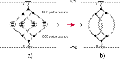
Figure 2: Scattering amplitude for the interaction of two dipoles with sizes: $r$ and $R$ at high energy in the MPSI approach (see Fig. 2-a and Fig. 2-b). The amplitudes of interaction of two dipoles in the Born approximation of perturbative QCD ( $N\left(r_{i},r^{\prime}_{i},b"_{i}\right)$ in Eq. (15)) are shown as white circles. The wavy lines denote the BFKL Pomerons. Fig. 2-c shows the Mueller diagramMUDIA for inclusive production of gluons.

The scattering amplitude in this approach can be written in the following formLELU2 :

$$N\left(Y,r,R,b\right)\,\, = \,\,-\,\,\sum^{\infty}_{n=1}\,\,(-1)^{n}\,\int\,\,\rho^{t}_{n}\left(\boldsymbol{r}_{1},\,\boldsymbol{b}^{\prime}_{1},\ldots\,,\boldsymbol{r}_{n},\,\boldsymbol{b}^{\prime}_{n};\,\frac{1}{2}Y\right)\,\,\rho^{p}_{n}\left(\boldsymbol{r}^{\prime}_{1},\,\boldsymbol{b}-\boldsymbol{b}^{\prime}_{1}-\boldsymbol{b}_{1}^{\prime\prime}\,,\ldots\,,\boldsymbol{r}_{n},\,\boldsymbol{b}-\boldsymbol{b}^{\prime}_{n}-\boldsymbol{b}_{n}^{\prime\prime};\,-\frac{1}{2}Y\right)$$ (15)

$$\times \,\prod^{n}_{i=1}\,\,d^{2}\,r_{i}\,\,\,\prod^{n}_{j=1}\,\,d^{2}\,r^{\prime}_{j}\,d^{2}b^{\prime}_{j}d^{2}b^{\prime\prime}_{j}\,N^{\rm BA}\left(r_{i},r^{\prime}_{i},b^{\prime\prime}_{i}\right)$$

where $\rho^{t}_{n}$ and $\rho^{p}_{n}$ denote the parton densities in the target and projectile, respectively. These densities can be calculated from $P_{n}$ using Eq. (11). $N^{\rm BA}$ is the scattering amplitude of two dipoles in the Born approximation of perturbative QCD (see Fig. 2). Eq. (15) simply states that we can consider the QCD parton cascade of Eq. (3) generated by the dipole of size $r$ for the c.m.f. rapidities from 0 to $\frac{1}{2}Y$, and the same cascade for the dipole of the size $R$, for the rapidities from 0 to $-\frac{1}{2}Y$. One can see that Eq. (15) is the $t$-channel unitarity re-written in a form, convenient for applying the evolution of the parton cascade in the form of Eq. (12).

Generally speaking, for a dense system of partons at $Y\,=\,0$ $n$-dipoles from upper cascade could interact with $m$ dipoles from the lower cascade, with the amplitude $N^{m}_{n}\left(\{r_{i}\},\{r^{\prime}_{j}\}\right)$ LELU2 . In Eq. (15) we assume that the system of dipoles that has been created at $Y=0$ is not very dense, at least for the range of rapidities given by Eq. (1). In this case

$$N^{m}_{n}\left(\{r_{i}\},\{r^{\prime}_{j}\}\right)\,\,=\,\,\delta_{n,m}\prod^{n}_{j=1}\,\left(-1\right)^{n-1}N^{\rm BA}\left(r_{i},r^{\prime}_{i},b^{\prime\prime}_{i}\right)$$ (16)

and after integration over $\{r_{1}\}$ and $\{r^{\prime}_{j}\}$, the scattering amplitude can be reduced to a system of enhanced BFKL Pomeron diagrams, which are shown in Fig. 2-b.

The average number of dipoles at $Y=0$ is determined by the inclusive cross section, which is given by the diagram of Fig. 2-c and which can be written at $y\to 0$ as followsKTINC :

$$\frac{d\sigma}{dy\,d^{2}p_{T}}=\frac{2C_{F}}{\alpha_{s}(2\pi)^{4}}\,\frac{1}{p^{2}_{T}}\int d^{2}\boldsymbol{r}_{T}\,e^{i\boldsymbol{p}_{T}\cdot\boldsymbol{r}_{T}}\!\!\int\!\!d^{2}b\,\nabla^{2}_{T}\,N^{\rm\mbox{\tiny BFKL}}\left(\frac{1}{2}Y;r,r_{T};b\right)\,\int\!\!d^{2}B\,\nabla^{2}_{T}\,N^{\rm\mbox{\tiny BFKL}}\left(y_{2}=-\frac{1}{2}Y;R,r_{T};B\right)$$ (17)

The average number of dipoles that enters the multiplicity distribution of Eq. (27), is equal $\bar{n}\,=\,N\,=\int\frac{d^{2}p_{T}}{(2\pi)^{2}}\frac{d\sigma}{dy\,d^{2}p_{T}}\Big{/}\sigma_{in}\,\propto\,\exp\left(\Delta_{\rm BFKL}\,Y\right)$ only if we assume that $\sigma_{in}\,\sim{\rm Const}$. Indeed, the enhanced diagrams of Fig. 2-b lead to the inelastic cross section which is constant at high energy.

II.3 Hadron - hadron collisions

In this paper we view a hadron as a dilute system of dipoles and use Eq. (17) for the average multiplicity, together with the multiplicity distribution of Eq. (1). In particular, we assume that Eq. (16) is correct, and the system of partons that is produced at c.m. rapidity $y^{*}$=0 is a dilute system. However, we are aware that Eq. (17) does not describe the experimental increase of the average multiplicity, which from Eq. (17) is $\bar{n}\,\propto\,\exp\left(\Delta_{\rm BFKL}\,Y\right)$. The experimental data can be described in the framework of the CGC/saturation approach in which $N^{\rm\mbox{\tiny BFKL}}$ were replaced by $N^{\rm\mbox{\tiny BK}}$LERE . Hence, we cannot view hadrons as a dilute system of dipoles, but rather have to consider them as a dense system of dipoles. For such a situation we expect that $\bar{n}\,\propto\,Q^{2}_{s}(Y)/\bar{\alpha}_{S}$ (see Refs.KOLEB ; KLN ; DKLN ; LERE ; LAPPI .

III Reggeon Field Theory in zero transverse dimensions.

III.1 Multiplicity distribution - a recap

In the parton modelFEYN ; BJP ; Gribov all partons have average transverse momentum which does not depend on energy. Therefore, we can obtain the parton model from the QCD cascade assuming that the unknown confinement of gluons leads to the QCD cascade for a dipole of fixed size. In this case the cascade equation (see Eq. (3)) takes the following simple form:

$$\frac{dP_{n}\left(Y\right)}{dY}\,\,=\,\,-\Delta\,n\,P_{n}\left(Y\right)\,\,+\,\,\left(n-1\right)\Delta P_{n-1}\left(Y.\right)$$ (18)

where $P_{n}\left(Y\right)$ denotes the probability to find $n$ dipoles (of a fixed size in our model) at rapidity $Y$, and $\Delta$ denotes the intercept of the BFKL Pomeron.

Instead of the generating functional of Eq. (6), we can introduce the generating function:

$$Z\left(Y,u\right)\,\,=\,\,\sum_{n}\,P_{n}\left(Y\right)\,u^{n}$$ (19)

where $u$ are numbers.

At the initial rapidity $Y=0$, we have only one dipole, so $P_{1}\left(Y=0\right)=1$ and $P_{n>1}\,=\,0$ (so the state is only one dipole); at $u=1$, $Z\left(Y,u=1\right)\,\,=\,\,\sum_{n}P\left(y\right)\,=\,1$. These two properties determine the initial and the boundary conditions for the generating function which simplify Eq. (7a) and Eq. (7b)

$$Z\left(Y=0,u\right)\,\,=\,\,u;~{}~{}~{}~{}~{}~{}~{}~{}~{}Z\left(Y,u=1\right)\,\,=\,\,1.$$ (20)

Eq. (18) takes the following form for the generating function:

$$\frac{\partial Z\left(Y,u\right)}{\partial Y}\,\,=\,\,-\Delta\,u\left(1-u\right)\frac{\partial Z\left(Y,u\right)}{\partial u}.$$ (21)

The general solution to Eq. (21) is an arbitrary function ($Z\left(z\right)$) of the new variable: $z\,\,=\,\,\Delta\,Y\,\,+\,\,f(u)$, with f(u) from the following equation:

$$1\,\,=\,\,-\,u\,\left(1\,-\,u\right)\,f^{\prime}_{u}\left(u\right)~{}~{}~{}~{}~{}f\left(u\right)\,\,=\,\,\ln\left(\frac{u\,-\,1}{u}\right)\,\,+\,\,C_{1}$$ (22)

The form of arbitrary function stems from the initial condition of Eq. (20)

$$Z\left(z\left(Y=0\right)\right)\,=\,u;$$ (23)

Since $u\,\,=\,\,1\Big{/}\left(1\,-\,e^{z}\right)$ we obtain that

$$Z\left(Y,\,u\right)\,\,=\,\,\frac{u\,\,e^{\,-\,\Delta\,Y}}{1\,\,+\,\,u\,\,\left(e^{\,-\,\Delta\,Y}\,-\,1\right)}\,\,=\,\,u\,e^{\,-\,\Delta\,Y}\,\sum^{\infty}_{n=1}\,u^{n}\left(1\,-\,e^{\,-\,\Delta\,Y}\right)^{n\,-\,1}.$$ (24)

Note, that $Z\left(Y,u=1\right)=1$, as it should be from Eq. (20).

On the other hand, we can re-write Eq. (21) in the form of the non-linear equation using Eq. (22): viz.

$$\,\,\frac{\partial\,Z}{\partial\,Y}\,\,=\,\,-\,\Delta\left(Z\,\,-\,\,Z^{2}\right).$$ (25)

Comparing Eq. (24) with Eq. (19) one can see that

$$P_{n}\left(Y\right)\,\,=\,\,e^{\,-\,\Delta\,Y}\left(1\,-\,e^{\,-\,\Delta\,Y}\right)^{n-1}.$$ (26)

Since from Eq. (26) it follows that the average $n\,=\,N$ is equal to $N\,=\exp\left(\Delta\,Y\right)$ Eq. (26) can be re-written in the form of Eq. (2):

$$P_{n}\left(N\right)\,\,=\,\,\frac{1}{N}\,\Big{(}1\,-\,\frac{1}{N}\Big{)}^{n-1}$$ (27)

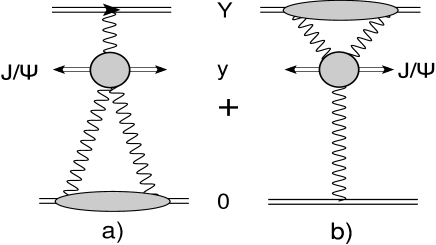
Figure 3: Mueller diagramsMUDIA for inclusive $J/\Psi$ production in the hadron-hadron collisions. The wavy lines denote the Pomeron Green’s functions.

III.2 Quarkonia production

As we have discussed in the introduction, we assume the production of heavy quakonia stems from three gluon fusion (see Fig. 1), and it is intimately related to the triple Pomeron interaction. The Mueller diagrams for inclusive $J/\Psi$ production are shown in Fig. 3, where the wavy lines denote the Pomeron Green’s function ($G_{I\!\!P}$) which is equal to

$$G_{I\!\!P}\left(Y\right)\,\,=\,\,e^{\Delta\,Y}$$ (28)

The MPSI approach for inclusive production with fixed multiplicity of produced hadrons is shown in Fig. 4

Therefore, from this figure we see that the structure of the parton cascade for the quarkonia production is quite different. In particular, for the part of the events whose weight is determined by the contribution of Fig. 3-b, the initial conditions for the parton cascade is not the ones of Eq. (20) however, they have the form:

$$Z\left(Y=0,u\right)\,\,=\,\,u^{2};~{}~{}~{}~{}~{}~{}~{}~{}~{}Z\left(Y,u=1\right)\,\,=\,\,1.$$ (29)

This means, that for this cascade we need to find the arbitrary function $Z\left(z\right)$ from the following equation

$$Z\left(z\left(Y=0\right)\right)\,=\,u^{2};$$ (30)

The solution is

$$Z\left(Y,u\right)\,\,=\,\,\frac{u^{2}\,e^{-2\,\Delta\,Y}}{\left(1\,\,+\,\,u\left(e^{-\,\Delta\,Y}\,\,-\,\,1\right)\right)^{2}}\,\,=\,\,u^{2}\,e^{\,-\,2\,\Delta\,Y}\,\sum^{\infty}_{n=1}\left(n\,-\,1\right)\,u^{n}\left(1\,-\,e^{\,-\,\Delta\,Y}\right)^{n-2}$$ (31)

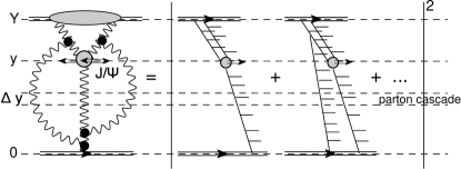
Fig. 4-a	Fig. 4-b

Figure 4: The example of Mueller diagramsMUDIA for inclusive $J/\Psi$ production in hadron-hadron collisions with fixed multiplicity of produced hadrons and the parton cascade, which they describe. The exchange of Pomerons do not cancel each other due to AGK cutting rulesAGK , since we fixed the multiplicity in the final state. The wavy lines denote the Pomeron Green’s functions. The black circles indicate the triple Pomeron vertices. The solid lines correspond to partons. $\Delta y$ is the rapidity window in which the multiplicity of the soft hadron is measured. This window is situated in central rapidity region with rapidity about $\frac{1}{2}Y$.

Eq. (31) leads to a different multiplicity distribution in comparison with Eq. (27): viz.

$$P^{(2)}_{n}\,\,=\,\,\frac{1}{N^{2}}\left(n\,\,-\,\,1\right)\left(1-\frac{1}{N}\right)^{n-2}$$ (32)

Finally, the cross section for quarkonia production with given multiplicity ($n$) of produced hadrons in the rapidity window $\Delta y$ (see Fig. 4), is equal to

$$\frac{d\sigma_{n}^{\rm J/\Psi}}{dy}\,\,\,=\,\,\frac{d\sigma^{\rm J/\Psi}_{\rm incl}}{dy}\left({Fig.~{}\ref{psipr}}-a\right)\frac{n}{\langle n^{(1)}\rangle}\,\,P^{(1)}_{n}\left(N\right)\,\,\,+\,\,\,\frac{d\sigma^{\rm J/\Psi}_{\rm incl}}{dy}\left({Fig.~{}\ref{psipr}}-b\right)\frac{n}{\langle n^{(2)}\rangle}\,\,P^{(2)}_{n}\left(N\right)$$ (33)

where $\langle n^{(1)}\rangle$ and $\langle n^{(2)}\rangle$ are average multiplicities of the produced hadrons in the parton cascades which are shown in Fig. 4-a and in Fig. 4-b, respectively.

In Eq. (33) the first and the second terms correspond to parton cascades that are shown in Fig. 4-a and in Fig. 4-b, respectively. The appearance of the factor $n/\langle n^{(i)}\rangle$ , which is the number of parton ladders, stems from the fact that $J/\Psi$ can be produced from every parton ladder (cut Pomeron) FEPA ; MTVW ; LSS . It should be stressed that the number of ladders at rapidity $y$ from which the $J/\Psi$ is produced, is the same as the number of ladders from which the soft hadrons are produced in the MPSI approachMPSI . It follows from the fact that integration over rapidities ($y^{\prime}$) of the triple Pomeron vertices in Fig. 4 leads to $Y-y^{\prime}\propto 1/\Delta$ for Pomerons in upper part of the diagram, and to $y^{\prime}\propto 1/\Delta$ in the lower part of the diagram. $\Delta$ denotes the Pomeron intercept.

Summing Eq. (33) we obtain that

$$\sum_{n}\frac{d\sigma_{n}^{\rm J/\Psi}}{dy}\,\,=\,\,\frac{d\sigma^{\rm J/\Psi}_{\rm incl}}{dy}\left({Fig.~{}\ref{psipr}}-a\right)\,\,+\,\,\frac{d\sigma^{\rm J/\Psi}_{\rm incl}}{dy}\left({Fig.~{}\ref{psipr}}-b\right)\,\,=\,\,\frac{d\sigma^{\rm J/\Psi}_{\rm incl}}{dy}$$ (34)

which coincide with the Mueller diagram approach, shown in Fig. 3. Introducing $\kappa\,\,=\frac{d\sigma^{\rm J/\Psi}_{\rm incl}}{dy}\left({Fig.~{}\ref{psipr}}-b\right)\Bigg{/}\frac{d\sigma^{\rm J/\Psi}_{\rm incl}}{dy}\left({Fig.~{}\ref{psipr}}-a\right)$ we re-write Eq. (33) in the following form:

$$\frac{\frac{d\sigma_{n}^{\rm J/\Psi}}{dy}}{\frac{d\sigma^{\rm J/\Psi}_{\rm incl}}{dy}}\,\,\,=\,\,\frac{1}{1\,\,+\,\,\kappa}\Bigg{(}\frac{n}{\langle n^{(1)}\rangle}\,\,P^{(1)}_{n}\left(N\right)\,\,\,+\,\,\,\kappa\frac{n}{\langle n^{(2)}\rangle}\,\,P^{(2)}_{n}\left(N\right)\Bigg{)}$$ (35)

where $\kappa$ is equal to LESI

$$\kappa\,\,=\,\,e^{2\,\Delta\left(\frac{1}{2}Y\,\,-\,\,y\right)}$$ (36)

In Eq. (33) $P^{(1)}_{n}\left(N\right)\,\,\equiv\,\,P_{n}\left(N\right)$ of Eq. (27).

The cross section of produced gluons (hadrons) is proportional to

$$\frac{d\sigma^{\rm prod.gl.}_{n}}{dy}\,\,=\,\,\,\,\frac{d\sigma^{\rm prod.gl.}_{\rm incl}}{dy}P^{(1)}_{n}\left(N\right)$$ (37)

From Fig. 5, one can see that $P^{(2)}_{n}\left(N\right)$ and $P^{(1)}_{n}\left(N\right)$ have different dependance on $z=n/N$. The average number of gluons is chosen to be the mean multiplicity of hadrons in the rapidity window $|\eta|\,\leq\,0.9$ measured at W=13TeV.

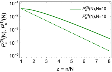
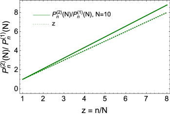
Fig. 5-a		Fig. 5-b

Figure 5: Fig. 5-a: $P^{(2)}_{n}\left(N\right)$ and $P^{(1)}_{n}\left(N\right)$ versus $z=\frac{n}{N}$. $N$ is taken to be equal 10. Fig. 5-b: The ratio of $P^{(2)}_{n}\left(N\right)/P^{(1)}_{n}\left(N\right)$ for $N=10$ and for large $N$ (see Eq. (39)

Therefore, $\frac{d\sigma^{\rm J/\Psi}}{dy}$ is not proportional to $\frac{d\sigma^{\rm prod.\,gl.i}}{dy}$, but shows non-linear dependance, which we will discuss below. It should be stressed that such dependance stems from triple Pomeron mechanism of quarkonia production, as noted in Refs.LESI ; LSS . At large $N$ we have

$$P^{(2)}_{n}\,\,\xrightarrow{N\,\gg\,1}\,\,\frac{1}{N}z\,e^{-z};~{}~{}~{}~{}~{}~{}~{}~{}P^{(1)}_{n}\,\,\xrightarrow{N\,\gg\,1}\,\,\frac{1}{N}\,e^{-z};$$ (38)

leading to

$$\frac{P^{(2)}_{n}}{P^{(1)}_{n}}\,\,\xrightarrow{N\,\gg\,1}\,\,z;$$ (39)

It is worth mentioning that the average multiplicity of $P^{(2)}$ distribution is equal to

$$<n^{(2)}>\,\,=\,\,\sum^{\infty}_{n=2}\,n\,P^{(2)}_{n}\left(N\right)\,\,=\,\,2\,N$$ (40)

Hence, for the multiplicity distribution $P^{(2)}$ the average number of accompanying gluons(hadrons) is twice larger than in the distribution $P^{(1)}$ . Eq. (40) means that the ratio $\frac{n^{(2)}}{<n^{(2)}>}\,\,=\,\,\frac{n}{2\,N}$.

IV Structure of QCD parton cascade

-

IV.1 Multiplicity distribution

In QCD, to find the multiplicity distribution for hadron-hadron scattering in QCD using MPSI approachMPSI , we need to evaluate (see Eq. (6))

$$\tilde{P}_{n}\left(Y,r\right)\,\,=\,\,\int P_{n}\left(Y,\boldsymbol{r},\boldsymbol{b};\{\boldsymbol{r}_{i}\,\boldsymbol{b}_{i}\}\right)\prod^{n}_{i=1}\,d^{2}r_{i}\,d^{2}b_{i}$$ (41)

However, in the MPSI approach it is more natural to introduce moments (see Eq. (12)):

$$M^{p}_{n}\left(Y,r\right)\,\,=\,\,\int_{r}\prod^{n}_{i=1}d^{2}r_{i}d^{2}b\,\rho^{p}_{n}\left(Y,\{r_{i}\},b\right)\,\,=\,\,\int_{r}\prod^{n}_{i=1}\frac{d^{2}r_{i}}{r^{2}_{i}}d^{2}b\,\bar{\rho}^{p}_{n}\left(Y,\{r_{i}\},b\right)$$ (42)

The integration over $r_{i}$ depends on the size of the initial dipole, which generates the cascade. In DIS the natural integration stems from $r_{i}\,>\,r$.

IV.1.1 Several first iterations.

We start from the first several iteration of Eq. (12), which can be re-written for $\,\bar{\rho}^{p}_{n}(r_{1},b_{1}\,\ldots\,,r_{n},b_{n})$ in the form

$$\frac{\partial\,\bar{\rho}^{p}_{n}(r_{1},b_{1}\,\ldots\,,r_{n},b_{n})}{\bar{\alpha}_{s}\,\partial\,Y}\,\, = \,\ -\,\sum_{i=1}^{n}\,\,\omega(r_{i})\,\,\bar{\rho}^{p}_{n}(r_{1},b_{1}\,\ldots\,,r_{n},b_{n})\,\,+\,\,2\,\sum_{i=1}^{n}\,\int\,\frac{d^{2}\,r^{\prime}}{2\,\pi}\,\frac{1}{(\boldsymbol{r}_{i}\,-\,\boldsymbol{r}^{\prime})^{2}}\,\bar{\rho}^{p}_{n}(\ldots\,r^{\prime},b_{i}-r^{\prime}/2\dots)$$ (43)

$$\,+\,\sum_{i=1}^{n-1}\,\bar{\rho}^{p}_{n-1}(\ldots\,(\boldsymbol{r}_{i}\,+\,\boldsymbol{r}_{n}),b_{in}\dots).$$

For the first iteration $\bar{\rho}_{1}\left(Y;r_{1},b_{1}\right)$, we obtain the BFKL equation:

$$\frac{\partial\,\bar{\rho}^{p}_{1}(Y;r_{1},b)}{\bar{\alpha}_{S}\,\partial\,Y}\,\,=\,\,-\,\,\omega_{G}\left(r_{1}\right)\bar{\rho}^{p}_{1}(Y;r_{1},b)\,\,+\,2\,\int\,\frac{d^{2}\,r^{\prime}}{2\,\pi}\,\frac{1}{(\boldsymbol{r}_{1}\,-\,\boldsymbol{r}^{\prime})^{2}}\,\bar{\rho}^{p}_{1}\left(Y,r^{\prime},b\right)\,\,=\,\,\int d^{2}\,r^{\prime}K\left(r_{1},r^{\prime}\right)\bar{\rho}^{p}_{1}\left(Y,r^{\prime},b\right)$$ (44)

with the solution

$$\bar{\rho}^{p}_{1}(Y;r_{1},b)\,\,=\,\,\int^{\epsilon\,+\,i\,\infty}_{\epsilon\,-\,i\,\infty}\frac{d\omega}{2\,\pi\,i}\int^{\epsilon\,+\,i\,\infty}_{\epsilon\,-\,i\,\infty}\frac{d\gamma}{2\,\pi\,i}\,e^{\omega\,Y\,\,+\,\,\gamma\,\xi_{1}}\frac{1}{\omega\,-\,\bar{\alpha}_{S}\chi\left(\gamma\right)}\tilde{\rho}^{p}_{in,1}(\gamma,b)$$ (45)

where $\xi_{1}\,\,=\,\,\ln\left(r^{2}_{1}\Lambda_{\rm QCD}^{2}\right)$ and

$$\omega\left(\gamma\right)\,\, = \,\,\bar{\alpha}_{S}\,\chi\left(\gamma\right)\,\,\,=\,\,\,\bar{\alpha}_{S}\left(2\psi\left(1\right)\,-\,\psi\left(\gamma\right)\,-\,\psi\left(1-\gamma\right)\right)$$ (46)

diffusion approximation $$\,\xrightarrow{\gamma\to\frac{1}{2}} \,\omega_{0}\,\,+\,\,D\,\left(\gamma-\frac{1}{2}\right)^{2}\,\,+\,\,{\cal O}\left((\gamma-\frac{1}{2})^{3}\right)\,\,$$

$$= \,\,\bar{\alpha}_{S}4\ln 2\,\,+\,\,\bar{\alpha}_{S}14\zeta\left(3\right)\left(\gamma-\frac{1}{2}\right)^{2}\,\,+\,\,{\cal O}\left((\gamma-\frac{1}{2})^{3}\right)$$

where $\psi(z)$ is Euler gamma function (see RY formula 8.36). $\tilde{\rho}^{p}_{in,1}(\gamma,b)$ has to be found from the initial conditions. From Eq. (45) we can obtain $M^{p}_{1}\left(Y,r,b\right)$ (see Eq. (42)) which has the following form:

$$M^{p}_{1}\left(Y,r\right)\,\,=\,\,\int^{\epsilon\,+\,i\,\infty}_{\epsilon\,-\,i\,\infty}\frac{d\omega}{2\,\pi\,i}\int^{\epsilon\,+\,i\,\infty}_{\epsilon\,-\,i\,\infty}\frac{d\gamma}{2\,\pi\,i}\,e^{\omega\,Y\,\,+\,\,\gamma\,\xi}\frac{1}{\omega\,-\,\bar{\alpha}_{S}\chi\left(\gamma\right)}M^{p}_{in,1}(\gamma)$$ (47)

which satisfies the following equation:

$$\frac{\partial\,M^{p}_{1}\left(Y,r\right)}{\partial\,\bar{\alpha}_{S}\,Y}\,\,=\,\,\,\,\,\int d^{2}\,r^{\prime}K\left(r,r^{\prime}\right)M^{p}_{1}\left(Y,r^{\prime}\right)\,\,\xrightarrow{r^{\prime}\,\gg\,r}\,\,\,\int_{r}\frac{d\,r^{\prime 2}}{r^{\prime 2}}\,\,M^{p}_{1}\left(Y,r^{\prime}\right)$$ (48)

The equation for the next iteration: $\bar{\rho}_{2}$, takes the form: Equation for $\rho^{p}_{2}$ can be re-written in the following form for $\bar{\rho}^{p}_{2}$:

$$\frac{\partial\,\bar{\rho}^{p}_{2}(Y;r_{1},r_{2},b)}{\bar{\alpha}_{S}\,\partial\,Y}\,\,=\,\,\int d^{2}\,r^{\prime}\,K\left(r_{1},r^{\prime}\right)\bar{\rho}^{p}_{2}\left(Y,r^{\prime},b,r_{2},b\right)\,+\,\,\,\int d^{2}\,r^{\prime}\,K\left(r_{2},r^{\prime}\right)\bar{\rho}^{p}_{2}\left(Y,r_{1},r^{\prime},b\right)\,\,+\,\,\bar{\rho}^{p}_{1}\left(Y;\boldsymbol{r}_{1}\,+\,\boldsymbol{r}_{2},b\right)$$ (49a)

$$~{}~{}~{}~{}~{}~{}~{}~{}~{}~{}~{}\xrightarrow{r^{\prime}\,\gg\,r_{i}}\int_{r_{1}}\frac{dr^{\prime 2}}{r^{\prime 2}}\bar{\rho}^{p}_{2}\left(Y,r^{\prime},b,r_{2},b\right)\,\,+\,\,\int_{r_{2}}\frac{dr^{\prime 2}}{r^{\prime 2}}\bar{\rho}^{p}_{2}\left(Y,r_{1},b,r^{\prime},b\right)\,\,+\,\,\bar{\rho}^{p}_{1}\left(Y;\boldsymbol{r}_{1}\,+\,\boldsymbol{r}_{2},b\right)$$ (49b)

For simplicity we re-write Eq. (49a) in the log approximation following Ref.GOLEMULT (see Eq. (49b)). Rewriting Eq. (49b) for $M^{p}_{2}$ we obtain:

$$\frac{\partial\,M^{p}_{2}(Y;r)}{\bar{\alpha}_{S}\,\partial\,Y}\,\,=\,\,\int_{r}\frac{dr^{\prime 2}}{r^{\prime 2}}\,\,\Bigg{\{}2\,M^{p}_{2}\left(Y,r^{\prime}\right)\,\,+\,\,M^{p}_{1}\left(Y,r^{\prime}\right)\Bigg{\}}\,\,=\,\,2\,\int_{r}\frac{dr^{\prime 2}}{r^{\prime 2}}\,\,\,M^{p}_{2}\left(Y,r^{\prime}\right)\,\,+\,\,\frac{\partial}{\partial\,\bar{\alpha}_{S}\,Y}M^{p}_{1}\left(Y,r\right)$$ (50)

In the last term of Eq. (50) we used Eq. (48). The solution to Eq. (50) takes the form:

$$M^{p}_{2}\left(Y,r\right)\,\,\,=\,\,\,\int^{\epsilon\,+\,i\,\infty}_{\epsilon\,-\,i\,\infty}\frac{d\omega}{2\,\pi\,i}\int^{\epsilon\,+\,i\,\infty}_{\epsilon\,-\,i\,\infty}\frac{d\gamma}{2\,\pi\,i}\,e^{\omega\,Y\,\,+\,\,\gamma\,\xi}\frac{\bar{\alpha}_{S}\chi\left(\gamma\right)}{\left(\omega\,\,-\,\,2\,\bar{\alpha}_{S}\chi\left(\gamma\right)\right)\,\left(\omega\,\,-\,\,\bar{\alpha}_{S}\chi\left(\gamma\right)\right)}$$ (51)

with $\chi\left(\gamma\right)=1/\gamma$. One can check that $M^{p}_{2}\left(Y,r\right)\,\xrightarrow{Y\,\to\,0}\,\,0$, which is the correct initial condition for one dipole of size $r$ at $Y=0$ , which generates the parton cascade. Actually, Eq. (50) describes $M^{p}_{2}\left(Y,r\right)$ for the full BFKL kernel. Indeed, considering Eq. (49a) we can integrate this equation over $r_{1}$ and $r_{2}$, to obtain the equation for $M^{p}_{2}$. The last term has the following form

$$\int_{r}\frac{d^{2}r_{1}}{2\,\pi}\frac{1}{r^{2}_{1}}\frac{d^{2}r_{2}}{2\,\pi}\int d^{2}b\frac{1}{r^{2}_{2}}\bar{\rho}(Y,r_{12},b)\,=\,\int_{r}\frac{d^{2}r_{1}}{2\,\pi}\frac{1}{r^{2}_{1}}\frac{d^{2}r_{2}}{2\,\pi}\int d^{2}b\,\frac{1}{\left(\boldsymbol{r}_{1}\,-\,\boldsymbol{r}_{12}\right)^{2}}\,\bar{\rho}(Y,r_{12},b)$$ (52)

Note that $r^{2}_{2}\,=\,\left(\boldsymbol{r}_{1}\,-\,\boldsymbol{r}_{12}\right)^{2}$ can never approach zero, since $r_{2}>r$. Removing this restriction, we can re-write

$$\int_{r}\frac{d^{2}r_{2}}{2\,\pi}\,\frac{1}{\left(\boldsymbol{r}_{1}\,-\,\boldsymbol{r}_{12}\right)^{2}}\,\bar{\rho}(Y,r_{12},b)\,\,=\,\,\int_{0}\frac{d^{2}r_{2}}{2\,\pi}\,\frac{1}{\left(\boldsymbol{r}_{1}\,-\,\boldsymbol{r}_{12}\right)^{2}}\,\bar{\rho}(Y,r_{12},b)\,\,-\,\,\ln r^{2}_{1}\,\bar{\rho}(Y,r_{1},b)$$ (53)

The reggeization term in Eq. (53) describes the contribution of $r_{2}\,\to\,0$. Plugging Eq. (53) in the last term of Eq. (49a) integrated over $r_{1}$ and $r_{2}$, one can see that we reproduce Eq. (50) for the full BFKL kernel. Hence Eq. (51) is the solution with $\chi\left(\gamma\right)$ which is given by Eq. (46).

IV.1.2 General solution

The equation for $M^{p}_{n}\left(Y,r\right)$ has the following general form:

$$\frac{\partial\,M^{p}_{n}(Y;r)}{\bar{\alpha}_{S}\,\partial\,Y}\,\,=$$ (54)

$$\,\,\int d^{2}\,r^{\prime}\,K\left(r,r^{\prime}\right)\,\,\Bigg{\{}n\,M^{p}_{2}\left(Y,r^{\prime}\right)\,\,+\,\,(n\,-\,1)M^{p}_{1}\left(Y,r^{\prime}\right)\Bigg{\}}\,\,=\,\,n\,\int d^{2}\,r^{\prime}\,K\left(r,r^{\prime}\right)\,\,\,M^{p}_{2}\left(Y,r^{\prime}\right)\,\,+\,\,\left(n\,-\,1\right)\frac{\partial}{\partial\,\bar{\alpha}_{S}\,Y}M^{p}_{1}\left(Y,r\right)$$

The solution to this equationGOLEMULT , which gives $M^{p}_{1}\left(Y=0,r\right)\,=\,1$, but all other $M^{p}_{n}$ with $n\,\geq\,2$=0, are equal to

$$M^{p}_{n}\left(Y,r\right)\,\,=\,\,\int^{\epsilon\,+\,i\,\infty}_{\epsilon\,-\,i\,\infty}\frac{d\gamma}{2\,\pi\,i}e^{\bar{\alpha}_{S}\chi\left(\gamma\right)\,Y}\,\Bigg{(}e^{\bar{\alpha}_{S}\chi\left(\gamma\right)\,Y}\,\,-\,\,1\Bigg{)}^{n-1}$$ (55)

which leads to the multiplicity distribution, which takes the form (see Eq. (41) and Ref.GOLEMULT ):

$$\tilde{P}_{n}\left(Y,r\right)\,\,\,=\,\,\int^{\epsilon\,+\,i\,\infty}_{\epsilon\,-\,i\,\infty}\frac{d\gamma}{2\,\pi\,i}\,e^{-\,\bar{\alpha}_{S}\chi\left(\gamma\right)\,Y}\,\Bigg{(}1\,\,-\,\,e^{-\,\bar{\alpha}_{S}\chi\left(\gamma\right)\,Y}\Bigg{)}^{n-1}$$ (56)

For $N\,\,=\,\,e^{\bar{\alpha}_{S}\chi\left(\gamma\right)\,Y}\,\,\gg\,\,1$ we have

$$\tilde{P}_{n}\left(Y,r\right)\,\,\,=\,\,\int^{\epsilon\,+\,i\,\infty}_{\epsilon\,-\,i\,\infty}\frac{d\gamma}{2\,\pi\,i}\,\exp\left(-z(\gamma)\,\,+\,\,\gamma\,\xi\right)~{}~{}~{}~{}\mbox{where}~{}~{}~{}~{}z\,\,=\,\,\frac{n}{e^{\bar{\alpha}_{S}\chi\left(\gamma\right)\,Y}}$$ (57)

Taking the integral over $\gamma$ using the method of steepest descent, using the diffusion approximation for the BFKL kernel (see Eq. (46)). The equation for $\gamma_{\rm SP}$ has the following form:

$$2\,D\,Yz\left(\frac{1}{2}\right)\left(\gamma_{\rm SP}\,-\,\frac{1}{2}\right)\,+\,\xi\,=0~{}~{}~{}~{}\mbox{with}~{}~{}~{}\left(\gamma_{\rm SP}\,-\,\frac{1}{2}\right)\,\,=\,\,-\,\frac{\xi}{2\,D\,Y\,z\left(\frac{1}{2}\right)}$$ (58)

and the integral over $\gamma$ is

$$\tilde{P}_{n}\left(Y,r\right)\,\,\,=\,\,\,\sqrt{\frac{\pi}{2\,D\,z\left(\frac{1}{2}\right)\,Y}}\,\frac{1}{N\left(Y\right)}\,e^{-z\left(\frac{1}{2}\right)}\,~{}~{}~{}\mbox{with}~{}~{}~{}~{}z\,=\,\frac{n}{N\left(Y\right)}~{}~{}~{}~{}\mbox{and}~{}~{}~{}N\left(Y\right)\,\,=\,\,e^{\omega_{0}\,Y}$$ (59)

considering $\xi^{2}\Big{/}2\,D\,z\left(\frac{1}{2}\right)Y\,\ll\,1$. After normalization, we obtain that

$$\frac{<n>\,\sigma_{n}}{\sigma_{\rm in}}\,\,\,=\Psi^{\rm KNO}\left(z\right)\,\,\,=\,\,\,\sqrt{\frac{1}{\pi\,z}}\,\,e^{-z\left(\frac{1}{2}\right)}\,~{}~{}~{}\mbox{with}~{}~{}~{}~{}z\,=\,\frac{n}{N\left(Y\right)}~{}~{}~{}~{}\mbox{and}~{}~{}~{}N\left(Y\right)\,\,=\,\,e^{\omega_{0}\,Y}$$ (60)

where $\Psi^{\rm KNO}$ denotes the KNO function (see Ref.KNO ).

It is worthwhile mentioning that the multiplicity distribution of Eq. (60) is different from Eq. (27) and

$$R\,=\,\frac{P_{n}^{\rm QCD}\left({Eq.~{}(\ref{QCDSOL4})}\right)}{P_{n}\left({Eq.~{}(\ref{NDIST})}\right)}\,\,=\,\,\sqrt{\frac{1}{\pi\,z}}$$ (61)

In Fig. 6 we compare the ALICE dataALICEMULT on multiplicity distribution with Eq. (59) and with Eq. (27). On can see that the agreement is good, and the difference between the above equations can be seen at large $n$. In describing the experimental data we use Eq. (59), which is derived at large $z$, for $z\,\geq\,3$. It worthwhile mentioning that the data of CMS CMSMULT we have discussed in our paperGOLEMULT .

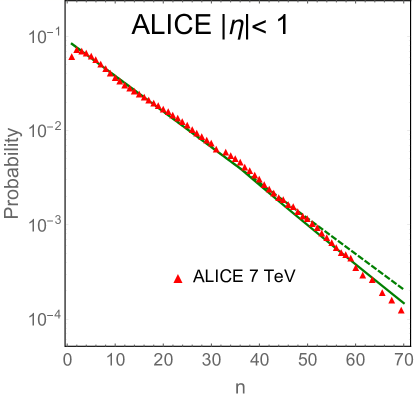
Figure 6: Multiplicity distribution of the charged hadrons in the central rapidity region. The solid line is the distribution of Eq. (59), while the dotted curve corresponds to Eq. (27). The data and the value of $N=12$ are taken from Refs.ALICEMULT .

IV.2 $P^{(2)}_{n}$ distribution for quarkonia production

The $P^{(1)}_{n}$ distribution , which we have discussed in the previous section, can be derived, using the double Laplace transform representation, both for $P^{(1)}_{n}\left(Y;r\right)$ and for $M^{(1)}_{n}\left(Y;r\right)$:

$$M^{(1)}_{n}\left(Y;r\right)\,\,\,=\,\,\,\int^{\epsilon\,+\,i\infty}_{\epsilon\,-\,i\,\infty}\frac{d\omega}{2\,\pi\,i}\int^{\epsilon\,+\,i\infty}_{\epsilon\,-\,i\,\infty}\frac{d\gamma}{2\,\pi\,i}\,e^{\omega\,Y\,\,+\,\,\gamma\,\xi}\,\,m^{(1)}_{n}\left(\omega,\gamma\right)$$ (62)

where $\xi\,=\,\ln\left(r^{2}\Lambda^{2}_{\rm QCD}\right)$.

Eq. (54) in the $\omega$-representation, has the following form:

$$\omega\,m^{(1)}_{n}\left(\omega,\gamma\right)\,\,\,=\,\,n\,\bar{\alpha}_{S}\chi\left(\gamma\right)\,m^{(1)}_{n}\left(\omega,\gamma\right)\,\,+\,\,\left(n-1\right)\,\bar{\alpha}_{S}\chi\left(\gamma\right)\,\,m^{(1)}_{n-1}\left(\omega,\gamma\right)$$ (63)

with the solution:

$$m^{(1)}_{n}\left(\omega,\gamma\right)\,\,\,=\,\,\left(n\,-\,1\right)!\prod^{n}_{m=1}\frac{\bar{\alpha}_{S}\chi\left(\gamma\right)}{\omega\,\,-\,\,m\,\bar{\alpha}_{S}\chi\left(\gamma\right)}$$ (64)

This solution gives $M^{p}_{1}\left(Y=0,r\right)\,\,\neq\,\,0$, while $M^{p}_{n}\left(Y=0,r\right)\,\,=\,\,0$ for $\,n\,\geq\,2$. The inverse Laplace transform leads to Eq. (55) for $M^{p}_{n}\left(Y,r\right)$ and Eq. (56) for $P^{(1)}_{n}\left(Y,r\right)$.

To find $P^{(2)}_{n}$ distribution we need to take into account that at $Y=0$:

$$M^{p}_{2}\left(Y=0,r\right)\,\,=\,\,1;~{}~{}~{}~{}~{}~{}~{}~{}M^{p}_{1}\left(Y=0,r\right)\,\,=\,\,0;~{}~{}~{}~{}~{}~{}~{}M^{p}_{n}\left(Y=0,r\right)\,\,=\,\,0~{}~{}\mbox{for}~{}~{}n\,\,\geq\,\,3$$ (65)

One can see that the following: $m^{(1)}_{1}\left(\omega,\gamma\right)$ satisfies thess conditions:

$$m^{(2)}_{n}\left(\omega,\gamma\right)\,\,\,=\,\,\left(n\,-\,1\right)!\prod^{n}_{m=2}\frac{\bar{\alpha}_{S}\chi\left(\gamma\right)}{\omega\,\,-\,\,m\,\bar{\alpha}_{S}\chi\left(\gamma\right)}$$ (66)

The inverse Laplace transform with respect to $\omega$ leads to

$$M^{(1)}_{n}\left(Y;r\right)\,\,\,=\,\,\,\int^{\epsilon\,+\,i\infty}_{\epsilon\,-\,i\,\infty}\frac{d\gamma}{2\,\pi\,i}\,e^{\gamma\,\xi}\,\,\frac{1}{\gamma}\,\left(n\,-\,1\right)\,e^{2\,\bar{\alpha}_{S}\,\chi\left(\gamma\right)\,Y}\,\Big{(}e^{2\,\bar{\alpha}_{S}\,\chi\left(\gamma\right)\,Y}\,\,-\,\,1\Big{)}^{n\,-\,2}$$ (67)

which gives the initial conditions of Eq. (65).

For $P^{(2)}_{n}$ we obtain

$$P^{(2)}_{n}\left(Y;r\right)\,\,\,=\,\,\,\int^{\epsilon\,+\,i\infty}_{\epsilon\,-\,i\,\infty}\frac{d\gamma}{2\,\pi\,i}\,e^{\gamma\,\xi}\,\,\frac{1}{\gamma}\,\left(n\,-\,1\right)\,e^{-\,2\,\bar{\alpha}_{S}\,\chi\left(\gamma\right)\,Y}\,\Big{(}1\,\,-\,\,e^{-2\,\bar{\alpha}_{S}\,\chi\left(\gamma\right)\,Y}\Big{)}^{n\,-\,2}$$ (68)

with $P^{(2)}_{2}\left(Y=0,r\right)\,\,=\,\,1$ and $P^{(2)}_{n}\left(Y=0,r\right)\,\,=\,\,0$ for $n\,\neq\,2$ at $Y=0$.

Repeating the same estimates as in Eq. (57), we obtain the KNO function,

$$\Psi^{KNO}\left(z\right)\,\,=\,\,2\,\sqrt{\frac{z}{\pi}}\,e^{-\,z}$$ (69)

with the normalization $\int dz\,\Psi^{KNO}\left(z\right)\,\,=\,\,1$.

Note that the ratio $\frac{P^{(2)}_{n}\left(Y,r\right)}{P^{(1)}_{n}\left(Y,r\right)}\,\,=\,\,z$ for large $z$, as in Eq. (39).

V Comparison with experimental data

In both ALICEALICE0 ; ALICE1 ; ALICE01 ; ALICE2 ; ALICE3 and STAR STAR1 ; STAR2 experiments the following ratio is measured:

$$\frac{n_{J/\Psi}}{\langle n_{J/\Psi}\rangle}\,\,=\,\,F\left(\frac{n}{N}\right)$$ (70)

where $N\,=\langle n\rangle$ is the average number of charged hadrons in the fixed rapidity window, and $\langle n^{J/\Psi}\rangle$ the average number of $J/\Psi$ which are measured generally speaking in a different rapidity window. It turns out that $F\left(\frac{n}{N}\right)\,\,\neq\,\,\frac{n}{N}$, but it is close to this when the rapidity windows are different. When both rapidity windows are the same, $F\left(\frac{n}{N}\right)$ shows much steeper dependence than $\frac{n}{N}$. In Ref.FEPA the $J/\Psi$ production is considered as being proportional to the number of collisions, since it comes from short distances, while the production of hadrons is proportional to the number of participants (see Ref.KLN .) However, in the framework of the CGC approach, the $J/\Psi$ production at high energies is proportional to the number of participantsLESI ; KHTU ; KLNT ; DKLMT as it can be seen from Fig. 1.

The main ingredients for describing the experimental data are Eq. (56)-Eq. (60) and Eq. (68)-Eq. (69), as well as Eq. (37). Using these equation we can re-write Eq. (35) in the form:

$$\frac{\frac{d\sigma_{n}^{\rm J/\Psi}}{dy}}{\frac{d\sigma^{\rm prod.gl.}_{n}}{dy}}\,\,\,=\,\,\frac{\frac{d\sigma_{\rm incl}^{\rm J/\Psi}}{dy}}{\frac{d\sigma^{\rm prod.gl.}_{\rm incl}}{dy}}\frac{1}{1\,\,+\,\,\kappa}\Bigg{(}\frac{n}{\langle n^{(1)}\rangle}\ \,\,\,+\,\,\,\kappa\frac{n}{\langle n^{(2)}\rangle}\,\,\frac{P^{(2)}_{n}\left(N\right)}{P^{(1)}_{n}\left(N\right)}\Bigg{)}\,\,=\,\,\frac{\frac{d\sigma_{\rm incl}^{\rm J/\Psi}}{dy}}{\frac{d\sigma^{\rm prod.gl.}_{\rm incl}}{dy}}\frac{1}{1\,\,+\,\,\kappa}\Bigg{(}\frac{n}{N}\ \,\,\,+\,\,\,\kappa\frac{n}{2\,N}\,\,\frac{P^{(2)}_{n}\left(N\right)}{P^{(1)}_{n}\left(N\right)}\Bigg{)}$$ (71)

Using Eq. (71) we can find the experimental observable (see Refs.ALICE1 ; LSS )

$$\displaystyle{\frac{dN_{J/\psi}/dy}{\langle dN_{J/\psi}/dy\rangle}\,\,=\frac{w\left(N_{J/\psi}\right)}{\left\langle w\left(N_{J/\psi}\right)\right\rangle}\,\frac{\left\langle w\left(N_{{\rm ch}}\right)\right\rangle}{w\left(N_{{\rm ch}}\right)}} =\frac{d\sigma_{J/\psi}\left(y,\,\eta,\,\sqrt{s},\,n\right)/dy}{d\sigma_{J/\psi}\left(y,\,\eta,\,\sqrt{s},\,n=N\right)/dy}/\frac{d\sigma_{{\rm ch}}\left(\eta,\,\sqrt{s},\,n\right)/d\eta}{d\sigma_{{\rm ch}}\left(\eta,\,\sqrt{s},\,n=N\right)/d\eta}$$ (72)

$$=\frac{\Bigg{(}\frac{n}{N}\ \,\,\,+\,\,\,\kappa\frac{n}{2\,N}\,\,\frac{P^{(2)}_{n}\left(N\right)}{P^{(1)}_{n}\left(N\right)}\Bigg{)}}{\Bigg{(}1\ \,\,\,+\,\,\,\frac{1}{2}\kappa\,\,\frac{P^{(2)}_{N}\left(N\right)}{P^{(1)}_{N}\left(N\right)}\Bigg{)}} \displaystyle{\xrightarrow{z=\frac{n}{N}\gg 1}\frac{z\,\,+\,\,\frac{\kappa}{4}\,z^{2}}{1+\frac{\kappa}{4}}}$$

In Fig. 7 we compare the experimental data with Eq. (72).

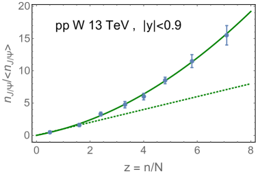
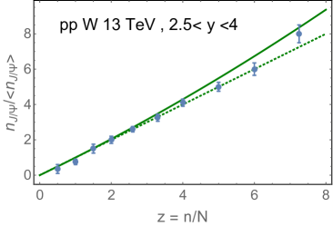
Fig. 7-a		Fig. 7-b

Figure 7: Comparison Eq. (72) with the experimental data of the ALICE collaborationALICE0 ; ALICE1 ; ALICE01 ; ALICE2 ; ALICE3 . The solid line is the estimate of Eq. (72), and the dotted line is the linear dependence which stems from the contribution of Fig. 4-a. Fig. 7-a shows the production of $J/\Psi$ in central rapidity region, while in Fig. 7-b the estimates are shown for Eq. (72) with $\kappa$ calculated in leading order of perturbative QCD, and with $\bar{\alpha}_{S}=0.15$.

One can see that this simple formula provides a fairly good description of the experimental data, for central production where $\kappa=1$. However, the experimental data for forward production of $J/\Psi$ALICE0 ; ALICE1 ; ALICE01 ; ALICE2 ; ALICE3 ; STAR1 ; STAR2 show almost a linear dependance: $\frac{n_{J/\Psi}}{\langle n_{J/\Psi}\rangle}\,\,=\,\,z$. Indeed, in Eq. (72) the quadratic term is suppressed, since it is proportional to the value of $\kappa$, which is equal to (see Fig. 4 and Ref.LESI for the estimates).

$$\kappa\,\,\,\,=\,\,\,\left(\frac{Q^{2}_{s}\left(Y-y\right)}{Q^{2}_{s}\left(y\right)}\right)^{\bar{\gamma}}\,\,=\,\,e^{-\,2\,\bar{\gamma}\lambda\,y^{*}}$$ (73)

where $y^{*}$ is the rapidity of the produced quarkonia in c.m.f. In leading order of perturbative QCD , in which we made all our previous estimatesKOLEB , $\bar{\gamma}\,\,=\,\,0.63$ and $\lambda\,=\,\bar{\alpha}_{S}\,\frac{\chi\left(\bar{\gamma}\right)}{\bar{\gamma}}\,\,\approx\,4.8\,\bar{\alpha}_{S}$. As is shown in Fig. 7-b, the estimate in leading order describes the data quite well. However, we need to remember that the NLO corrections both to $\bar{\gamma}$ and to $\lambda$ are large.

VI Conclusions

In this paper we re-visited the problem of multiplicity distributions in high energy QCD, which we have discussed in Ref.GOLEMULT and found the distribution of Eq. (59). This distribution provides a better description of the experimental data at large multiplicities $n$, than Eq. (27), which has been discussed previously. We also suggest a different approach to the multiplicity dependence of quarkonia production. It should be stressed that our approach is based on the three gluons fusion mechanism of Fig. 1, and it differs from the description of Refs.MTVW ; LSS , since we did not assume the multiplicity dependence of the saturation scale. In our approach we assume, that the production of $J/\Psi$, which occurs at rapidity $y$, and the central production of charged hadrons, stem from the production of the same $n$-parton cascades, which are pictured in Fig. 8 as the production of $n$-gluon ladders. Solving the QCD cascade equation, we found the multiplicity distribution both for the cascade of Fig. 8-a (see Eq. (68) - Eq. (69)) and for the cascade of Fig. 8-b (see Eq. (56) - Eq. (60)) .

In Fig. 8 one can see that $J/\Psi$ can be produced from each of $n$-ladders, leading to the cross section, which is proportional to $n$ (see Fig. 8-a). This mechanism is shown in Fig. 3-a. However, $J/\Psi$ can be created from merging of two ladders (see Fig. 8-b) , which gives a cross section $\propto\,\,n^{2}$, and corresponds to Fig. 3-b. Note, that the production of the hadrons in both cases can be found from Eq. (37). Taking into account that the average number of gluons (hadrons) for the mechanism of Fig. 8-b is two time larger than for Fig. 8-a, we infer that Fig. 8 leads to the simple Eq. (72).

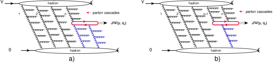
Figure 8: The production of quarkonia from $n$ parton cascades.

It should be stressed that this equation is heavily dependent on the three gluon fusion mechanism, but does not depend on the details of the cross section of quakonia production. In particular, as we have mentioned above, we do not use the dependence of the saturation scale on the multiplicity of the produced gluons. This means that the non-linear dependence of $J/\Psi$-production on multiplicity of charged hadrons, can stem from sources other than the dependence of the cross section on the saturation scale. Actually, this statement follows directly from the fact that 1+1 RFT generates the non-linear dependence on $n$.

It should be noted that if we assume, that in addition to the three gluon fusion mechanism we have the production of $J/\Psi$ from color-singlet model, we will not obtain agreement with the description of the experimental data in Fig. 7.

As an aside, we note in MTVW ; LSS it was assumed that the $J/\Psi$-production results from the inclusive diagrams of Fig. 3-a and Fig. 3-b. This is erroneous, as at arbitrary $n$ it is necessary to include the production of many partonic showers as illustrated in Fig. 4-a and Fig. 4-b. The difference to the percolation approachFEPA , lies in our hypothesis that both the production of $J/\Psi$ and the charged pion stem from short distances of the order of $r\,\propto\,1/Q_{s}$, and are determined by physics controlled by the CGC effective theory. The gluon jets with transverse momentum $Q_{s}$, decay into charged pions (see Ref.LSS for details). The non-linear dependence of production of $J/\Psi$ is due to the three Pomeron fusion mechanism.

In spite of the good description of the experimental data for the quarkonia production integrated over the transverse momenta ($p_{T}$), we cannot explain at present, why the data at fixed $p_{T}$ ALICE0 , shows a steeper dependence on $n$ than the integrated data. Certainly, this problem will be the main subject of our further attempts to understand the multiplicity dependence of quarkonia production.

VII Acknowledgements

We thank our colleagues at Tel Aviv university and UTFSM for encouraging discussions. This research was supported by ANID PIA/APOYO AFB180002 (Chile) and Fondecyt (Chile) grants 1180118.

References

• (1) Yuri V. Kovchegov and Eugene Levin, “ Quantum Chromodynamics at High Energies", Cambridge Monographs on Particle Physics, Nuclear Physics and Cosmology, Cambridge University Press, 2012 .
• (2) L. McLerran and R. Venugopalan, “Computing quark and gluon distribution functions for very large nuclei", Phys. Rev. D49 (1994) 2233, “Gluon distribution functions for very large nuclei at small transverse momentum", Phys. Rev. D49 (1994), 3352; ‘Green’s function in the color field of a large nucleus", D50 (1994) 2225; “ Fock space distributions, structure functions, higher twists, and small $x$" , D59 (1999) 09400.
• (3) A. H. Mueller, “Soft Gluons In The Infinite Momentum Wave Function And The BFKL Pomeron,” Nucl. Phys.  B 415, 373 (1994);   “Unitarity and the BFKL pomeron,” Nucl. Phys.  B 437 (1995) 107 [arXiv:hep-ph/9408245].
• (4) I. Balitsky, “Operator expansion for high-energy scattering", [arXiv:hep-ph/9509348];   “Factorization and high-energy effective action", Phys. Rev. D60, 014020 (1999) [arXiv:hep-ph/9812311].
• (5) Y. V. Kovchegov, “ Small-x $F_{2}$ structure function of a nucleus including multiple Pomeron exchanges"’ Phys. Rev. D60, 034008 (1999), [arXiv:hep-ph/9901281].
• (6) J. Jalilian-Marian, A. Kovner, A. Leonidov, and H. Weigert, “The BFKL equation from the Wilson renormalization group" , Nucl. Phys. B504 (1997) 415–431, [ arXiv:hep-ph/9701284];   J. Jalilian-Marian, A. Kovner, A. Leonidov, and H. Weigert, “The Wilson renormalization group for low x physics: Towards the high density regime" , Phys.Rev. D59 (1998) 014014, [arXiv:hep-ph/9706377 [hep-ph]];    A. Kovner, J. G. Milhano, and H. Weigert, “Relating different approaches to nonlinear QCD evolution at finite gluon density" , Phys. Rev. D62 (2000) 114005, [ arXiv:hep-ph/0004014];    E. Iancu, A. Leonidov, and L. D. McLerran, Nonlinear gluon evolution in the color glass condensate. I" ,Nucl. Phys. A692 (2001) 583–645, [ arXiv:hep-ph/0011241];    E. Iancu, A. Leonidov, and L. D. McLerran, “The renormalization group equation for the color glass condensate" , Phys. Lett. B510 (2001) 133–144, [ arXiv:hep-ph/0102009];   E. Ferreiro, E. Iancu, A. Leonidov, and L. McLerran, “Nonlinear gluon evolution in the color glass condensate. II" , Nucl. Phys. A703 (2002) 489–538, [ arXiv:hep-ph/0109115];    H. Weigert, Unitarity at small Bjorken $x$, Nucl. Phys. A703, 823 (2002), [arXiv:hep-ph/0004044].
• (7) F. Gelis, E. Iancu, J. Jalilian-Marian and R. Venugopalan, “The Color Glass Condensate,” Ann. Rev. Nucl. Part. Sci. 60 (2010), 463-489 doi:10.1146/annurev.nucl.010909.083629 [arXiv:1002.0333 [hep-ph]].
• (8) V. S. Fadin, E. A. Kuraev and L. N. Lipatov, “On the pomeranchuk singularity in asymptotically free theories", Phys. Lett. B60, 50 (1975);    E. A. Kuraev, L. N. Lipatov and V. S. Fadin, “The Pomeranchuk Singularity in Nonabelian Gauge Theories" Sov. Phys. JETP 45, 199 (1977), [Zh. Eksp. Teor. Fiz.72,377(1977)];    “The Pomeranchuk Singularity in Quantum Chromodynamics,” I. I. Balitsky and L. N. Lipatov, Sov. J. Nucl. Phys. 28, 822 (1978), [Yad. Fiz.28,1597(1978)].
• (9) L. N. Lipatov, “The Bare Pomeron in Quantum Chromodynamics,” Sov. Phys. JETP 63, 904 (1986) [Zh. Eksp. Teor. Fiz.  90, 1536 (1986)].
• (10) L. V. Gribov, E. M. Levin and M. G. Ryskin, “Semihard Processes in QCD,” Phys. Rept.  100, 1 (1983). doi:10.1016/0370-1573(83)90022-4
• (11) E. M. Levin and M. G. Ryskin, “High-energy hadron collisions in QCD,” Phys. Rept.  189, 267 (1990).
• (12) A. H. Mueller and J. Qiu, “ Gluon recombination and shadowing at small values of $x$", Nucl. Phys. B268 (1986) 427.
• (13) A. H. Mueller and B. Patel, “Single and double BFKL pomeron exchange and a dipole picture of high-energy hard processes", Nucl. Phys. B425 (1994) 471.
• (14) J. Bartels, M. Braun and G. Vacca, “Pomeron vertices in perturbative QCD in diffractive scattering,” Eur. Phys. J. C 40 (2005), 419-433 doi:10.1140/epjc/s2005-02152-x [arXiv:hep-ph/0412218 [hep-ph]];   J. Bartels and C. Ewerz, “Unitarity corrections in high-energy QCD,” JHEP 09 (1999), 026 doi:10.1088/1126-6708/1999/09/026 [arXiv:hep-ph/9908454 [hep-ph]];    J. Bartels and M. Wusthoff, “The Triple Regge limit of diffractive dissociation in deep inelastic scattering,” Z. Phys. C 66 (1995), 157-180 doi:10.1007/BF01496591; J. Bartels, “Unitarity corrections to the Lipatov pomeron and the four gluon operator in deep inelastic scattering in QCD,” Z. Phys. C 60 (1993), 471-488 doi:10.1007/BF01560045
• (15) M. Braun, “Conformal invariant pomeron interaction in the perurbative QCD with large $N_{c}$,” Phys. Lett. B 632 (2006), 297-304 doi:10.1016/j.physletb.2005.10.054 [arXiv:hep-ph/0512057 [hep-ph]];    “Nucleus nucleus interaction in the perturbative QCD,” Eur. Phys. J. C 33 (2004), 113-122 doi:10.1140/epjc/s2003-01565-9 [arXiv:hep-ph/0309293 [hep-ph]]; “Nucleus-nucleus scattering in perturbative QCD with $N_{c}\to$ infinity,” Phys. Lett. B 483 (2000), 115-123 doi:10.1016/S0370-2693(00)00571-2 [arXiv:hep-ph/0003004 [hep-ph]];   “Structure function of the nucleus in the perturbative QCD with $N_{c}\to$ infinity (BFKL pomeron fan diagrams),” Eur. Phys. J. C 16 (2000), 337-347 doi:10.1007/s100520050026 [arXiv:hep-ph/0001268 [hep-ph]];   “The system of four reggeized gluons and the three-pomeron vertex in the high colour limit" Eur. Phys. J. C6, 321 (1999) [arXiv:hep-ph/9706373];   M. Braun and G. Vacca, “Triple pomeron vertex in the limit $N_{c}\to$ infinity,” Eur. Phys. J. C 6 (1999), 147-157 doi:10.1007/s100520050328 [arXiv:hep-ph/9711486 [hep-ph]].
• (16) Y. V. Kovchegov and E. Levin, “Diffractive dissociation including multiple pomeron exchanges in high parton density QCD,” Nucl. Phys. B 577 (2000), 221-239 doi:10.1016/S0550-3213(00)00125-5 [arXiv:hep-ph/9911523 [hep-ph]].
• (17) E. Levin and M. Lublinsky, “Towards a symmetric approach to high energy evolution: Generating functional with Pomeron loops,” Nucl. Phys.  A 763 (2005) 172 [arXiv:hep-ph/0501173].
• (18) E. Levin and M. Lublinsky, “Balitsky’s hierarchy from Mueller’s dipole model and more about target correlations,” Phys. Lett.  B 607 (2005) 131 [arXiv:hep-ph/0411121];   “A linear evolution for non-linear dynamics and correlations in realistic nuclei,” Nucl. Phys.  A 730 (2004) 191 [arXiv:hep-ph/0308279].
• (19) E. Levin, J. Miller and A. Prygarin, “Summing Pomeron loops in the dipole approach,” Nucl. Phys.  A806 (2008) 245, [arXiv:0706.2944 [hep-ph]].
• (20) T. Altinoluk, C. Contreras, A. Kovner, E. Levin, M. Lublinsky and A. Shulkim, “QCD reggeon calculus from JIMWLK Evolution,” Int. J. Mod. Phys. Conf. Ser.  25 (2014) 1460025;    T. Altinoluk, N. Armesto, A. Kovner, E. Levin and M. Lublinsky, “KLWMIJ Reggeon field theory beyond the large $N_{c}$ limit,” JHEP 1408 (2014) 007.
• (21) T. Altinoluk, A. Kovner, E. Levin and M. Lublinsky, “Reggeon Field Theory for Large Pomeron Loops,” JHEP 1404 (2014) 075 [arXiv:1401.7431 [hep-ph]].;    T. Altinoluk, C. Contreras, A. Kovner, E. Levin, M. Lublinsky and A. Shulkin, “QCD Reggeon Calculus From KLWMIJ/JIMWLK Evolution: Vertices, Reggeization and All,” JHEP 1309 (2013) 115.
• (22) E. Levin, “Dipole-dipole scattering in CGC/saturation approach at high energy: summing Pomeron loops,’ JHEP 1311 (2013) 039 [arXiv:1308.5052 [hep-ph]].
• (23) A. Kovner, M. Lublinsky and U. Wiedemann, “From bubbles to foam: Dilute to dense evolution of hadronic wave function at high energy,” JHEP 06 (2007), 075 doi:10.1088/1126-6708/2007/06/075 [arXiv:0705.1713 [hep-ph]].
• (24) T. Altinoluk, A. Kovner, M. Lublinsky and J. Peressutti, “QCD Reggeon Field Theory for every day: Pomeron loops included,” JHEP 03 (2009), 109 doi:10.1088/1126-6708/2009/03/109 [arXiv:0901.2559 [hep-ph]].
• (25) A. H. Mueller and B. Patel, “Single and double BFKL pomeron exchange and a dipole picture of high-energy hard processes,” Nucl. Phys. B 425, 471-488 (1994) doi:10.1016/0550-3213(94)90284-4 [arXiv:hep-ph/9403256 [hep-ph]]. A. H. Mueller and G. Salam, “Large multiplicity fluctuations and saturation effects in onium collisions,” Nucl. Phys. B 475 (1996), 293-320 doi:10.1016/0550-3213(96)00336-7 [arXiv:hep-ph/9605302 [hep-ph]];    G. Salam, “Studies of unitarity at small x using the dipole formulation,” Nucl. Phys. B 461 (1996), 512-538 doi:10.1016/0550-3213(95)00658-3 [arXiv:hep-ph/9509353 [hep-ph]];    E. Iancu and A. Mueller, “Rare fluctuations and the high-energy limit of the S matrix in QCD,” Nucl. Phys. A 730 (2004), 494-513 doi:10.1016/j.nuclphysa.2003.10.019 [arXiv:hep-ph/0309276 [hep-ph]];   “From color glass to color dipoles in high-energy onium onium scattering,” Nucl. Phys. A 730 (2004), 460-493 doi:10.1016/j.nuclphysa.2003.10.017 [arXiv:hep-ph/0308315 [hep-ph]].
• (26) S. Acharya et al. [ALICE], “Multiplicity dependence of J/$\psi$ production at midrapidity in pp collisions at $\sqrt{s}$ = 13 TeV,” [arXiv:2005.11123 [nucl-ex]].
• (27) D. Thakur [ALICE], $J/\psi$ production as a function of charged-particle multiplicity with ALICE at the LHC,” Springer Proc. Phys. 234, 217-221 (2019), [arXiv:1811.01535 [hep-ex]].
• (28) C. Jahnke [ALICE], “J/$\psi$ production as a function of event multiplicity in pp collisions at $\sqrt{s}$ = 13 TeV using EMCal-triggered events with ALICE at the LHC,” [arXiv:1805.00841 [hep-ex]].
• (29) J. Adam et al. [ALICE], “Measurement of charm and beauty production at central rapidity versus charged-particle multiplicity in proton-proton collisions at $\sqrt{s}=7$ TeV,” JHEP 09, 148 (2015) doi:10.1007/JHEP09(2015)148 [arXiv:1505.00664 [nucl-ex]].
• (30) B. Abelev et al. [ALICE Collaboration], $J/\psi$ production as a function of charged particle multiplicity in pp collisions at $\sqrt{s}$=7 TeV", Phys. Lett. B 712 (2012), 165. [arXiv:1202.2816 [hep-ex]].
• (31) B. Trzeciak [STAR], $J/\psi$ and $\psi(2S)$ measurement in p+p collisions $\sqrt{s}=$ 200 and 500 GeV with the STAR experiment,” J. Phys. Conf. Ser. 668, no.1, 012093 (2016) doi:10.1088/1742-6596/668/1/012093 [arXiv:1512.07398 [hep-ex]].
• (32) R. Ma [STAR], “Measurement of $J/\Psi$ production in p + p collisions at s=500 GeV at STAR experiment,” Nucl. Part. Phys. Proc. 276-278, 261-264 (2016) doi:10.1016/j.nuclphysbps.2016.05.059 [arXiv:1509.06440 [nucl-ex]].
• (33) B. Kopeliovich, H. Pirner, I. Potashnikova, K. Reygers and I. Schmidt, $J/\Psi$ in high-multiplicity pp collisions: Lessons from pA collisions,” Phys. Rev. D 88, no.11, 116002 (2013) doi:10.1103/PhysRevD.88.116002 [arXiv:1308.3638 [hep-ph]].
• (34) E. Ferreiro and C. Pajares, “High multiplicity $pp$ events and $J/\psi$ production at LHC,” Phys. Rev. C 86, 034903 (2012) doi:10.1103/PhysRevC.86.034903 [arXiv:1203.5936 [hep-ph]].
• (35) E. Levin and M. Siddikov, $J/\psi$ production in hadron scattering: three-pomeron contribution,” Eur. Phys. J. C 79, no.5, 376 (2019) doi:10.1140/epjc/s10052-019-6894-1 [arXiv:1812.06783 [hep-ph]].
• (36) Y. Q. Ma, P. Tribedy, R. Venugopalan and K. Watanabe, “Event engineering studies for heavy flavor production and hadronization in high multiplicity hadron-hadron and hadron-nucleus collisions,” Phys. Rev. D 98 (2018) no.7, 074025 doi:10.1103/PhysRevD.98.074025 [arXiv:1803.11093 [hep-ph]].
• (37) E. Levin, I.  Schmidt, I. and M. Siddikov, “Multiplicity distributions as probes of quarkonia production mechanisms,” Eur. Phys. J. C 80, no.6, 560 (2020) doi:10.1140/epjc/s10052-020-8086-4 [arXiv:1910.13579 [hep-ph]].
• (38) A. H. Mueller, “O(2,1) analysis of single particle spectra at high energy,” Phys. Rev. D2 (1970) 2963.
• (39) V. A. Khoze, A. D. Martin, M. G. Ryskin and W. J. Stirling, “Inelastic $J/\psi$ and $\Upsilon$ hadroproduction,” Eur. Phys. J. C 39, 163 (2005), [hep-ph/0410020].
• (40) L. Motyka and M. Sadzikowski, “On relevance of triple gluon fusion in $J/\psi$ hadroproduction,” Eur. Phys. J. C 75 (2015) no.5, [arXiv:1501.04915 [hep-ph]]
• (41) D. Kharzeev and K. Tuchin, “Signatures of the color glass condensate in J/psi production off nuclear targets,” Nucl. Phys. A 770 (2006) 40, [hep-ph/0510358].
• (42) D. Kharzeev, E. Levin, M. Nardi and K. Tuchin, “Gluon saturation effects on J/Psi production in heavy ion collisions”, Phys. Rev. Lett. 102 (2009) 152301, [arXiv:0808.2954 [hep-ph]]; “J/Psi production in heavy ion collisions and gluon saturation,” Nucl. Phys. A 826 (2009) 230, [arXiv:0809.2933 [hep-ph]].
• (43) F. Dominguez, D. E. Kharzeev, E. Levin, A. H. Mueller and K. Tuchin, “Gluon saturation effects on the color singlet J/$\psi$ production in high energy dA and AA collisions,” Phys. Lett. B 710 (2012) 182, [arXiv:1109.1250 [hep-ph]].
• (44) D. E. Kharzeev, E. M. Levin and K. Tuchin, “Nuclear modification of the J/$\psi$ transverse momentum distributions in high energy pA and AA collisions,” Nucl. Phys. A 924 (2014) 47 doi:10.1016/j.nuclphysa.2014.01.006 [arXiv:1205.1554 [hep-ph]].
• (45) Z. B. Kang, Y. Q. Ma and R. Venugopalan, “Quarkonium production in high energy proton-nucleus collisions: CGC meets NRQCD,” JHEP 1401 (2014) 056, [arXiv:1309.7337 [hep-ph]].
• (46) E. Gotsman and E. Levin, “High energy QCD: multiplicity distribution and entanglement entropy,” [arXiv:2006.11793 [hep-ph]].
• (47) D. E. Kharzeev and E. M. Levin, “Deep inelastic scattering as a probe of entanglement,” Phys. Rev. D 95 (2017) no.11, 114008 doi:10.1103/PhysRevD.95.114008 [arXiv:1702.03489 [hep-ph]].
• (48) Y. V. Kovchegov and K. Tuchin, “Inclusive gluon production in DIS at high parton density,” Phys. Rev.  D65 (2002) 074026 [arXiv:hep-ph/0111362].
• (49) D. Kharzeev and M. Nardi, “Hadron production in nuclear collisions at RHIC and high density QCD,” Phys. Lett. B 507, 121 (2001) [nucl-th/0012025]. . D. Kharzeev and E. Levin, ‘ ‘Manifestations of high density QCD in the first RHIC data,” Phys. Lett. B 523 (2001) 79, [nucl-th/0108006];   D. Kharzeev, E. Levin and M. Nardi, “The Onset of classical QCD dynamics in relativistic heavy ion collisions,” Phys. Rev. C 71 (2005) 054903, [hep-ph/0111315]; “Hadron multiplicities at the LHC,” J. Phys. G 35 (2008) no.5, 054001.38 [arXiv:0707.0811 [hep-ph]].
• (50) A. Dumitru, D. E. Kharzeev, E. M. Levin and Y. Nara, “ “Gluon Saturation in $pA$ Collisions at the LHC: KLN Model Predictions For Hadron Multiplicities,” Phys. Rev. C 85 (2012) 044920 [arXiv:1111.3031 [hep-ph]]
• (51) E. Levin and A. H. Rezaeian, “Gluon saturation and inclusive hadron production at LHC,” Phys. Rev. D 82 (2010), 014022 doi:10.1103/PhysRevD.82.014022 [arXiv:1005.0631 [hep-ph]].
• (52) T. Lappi, “Energy dependence of the saturation scale and the charged multiplicity in pp and AA collisions,” Eur. Phys. J. C 71, 1699 (2011) [arXiv:1104.3725 [hep-ph]].
• (53) R.P. Feynman, “Very high-energy collisions of hadrons,” Phys. Rev. Lett.  23, 1415 (1969).     “Photon-hadron interactions,” Reading 1972. Photon-Hadron Interactions, Reading, 1972.
• (54) J.D. Bjorken and E.A. Paschos,“Inelastic Electron-Proton and $\gamma$ -Proton Scattering and the Structure of the Nucleon," Phys. Rev. 185, 1975(1969).
• (55) V.N. Gribov, “Inelastic processes at super high-energies and the problem of nuclear cross-sections,” Sov. J. Nucl. Phys.  9, 369 (1969) [Yad. Fiz.  9, 640 (1969)];    “Space-time description of hadron interactions at high-energies,” Proc. ITEP School on Elementary particle physics, v.1, p.65 (1973); hep-ph/0006158.
• (56) V. A. Abramovsky, V. N. Gribov and O. V. Kancheli, “Character of Inclusive Spectra and Fluctuations Produced in Inelastic Processes by Multi - Pomeron Exchange,” Yad. Fiz. 18, 595-616 (1973),[Sov.J.Nucl.Phys. 18 (1974) 308-317].
• (57) I. Gradstein and I. Ryzhik, Table of Integrals, Series, and Products, Fifth Edition, Academic Press, London, 1994.
• (58) Z. Koba, H. B. Nielsen and P. Olesen, “Scaling of multiplicity distributions in high-energy hadron collisions,” Nucl. Phys. B 40 (1972), 317-334 doi:10.1016/0550-3213(72)90551-2
• (59) K. Aamodt et al. [ALICE], “Charged-particle multiplicity measurement in proton-proton collisions at $\sqrt{s}=7$ TeV with ALICE at LHC,” Eur. Phys. J. C 68, 345-354 (2010) doi:10.1140/epjc/s10052-010-1350-2 [arXiv:1004.3514 [hep-ex]].
• (60) V. Khachatryan et al. [CMS], “Charged Particle Multiplicities in $pp$ Interactions at $\sqrt{s}=0.9$, 2.36, and 7 TeV,” JHEP 01, 079 (2011) doi:10.1007/JHEP01(2011)079 [arXiv:1011.5531 [hep-ex]].
• (61) O. Baker and D. Kharzeev, “Thermal radiation and entanglement in proton-proton collisions at energies available at the CERN Large Hadron Collider,” Phys. Rev. D 98 (2018) no.5, 054007 doi:10.1103/PhysRevD.98.054007 [arXiv:1712.04558 [hep-ph]].
• (62) E. Gotsman and E. Levin, “Thermal radiation and inclusive production in the CGC/saturation approach at high energies,” Eur. Phys. J. C 79 (2019) no.5, 415 doi:10.1140/epjc/s10052-019-6923-0 [arXiv:1902.07923 [hep-ph]].
• (63) E. Gotsman and E. Levin, “Thermal radiation and inclusive production in the Kharzeev-Levin-Nardi model for ion-ion collisions,” Phys. Rev. D 100 (2019) no.3, 034013 doi:10.1103/PhysRevD.100.034013 [arXiv:1905.05167 [hep-ph]].
• (64) Z. Tu, D. E. Kharzeev and T. Ullrich, “Einstein-Podolsky-Rosen Paradox and Quantum Entanglement at Subnucleonic Scales,” Phys. Rev. Lett. 124 (2020) no.6, 062001 doi:10.1103/PhysRevLett.124.062001 [arXiv:1904.11974 [hep-ph]].
• (65) A. Kovner, E. Levin and M. Lublinsky, “QCD unitarity constraints on Reggeon Field Theory,” JHEP 08 (2016), 031 doi:10.1007/JHEP08(2016)031 [arXiv:1605.03251 [hep-ph]].
• (66) E. Gotsman, A. Kormilitzin, E. Levin and U. Maor, “QCD motivated approach to soft interactions at high energies: nucleus-nucleus and hadron-nucleus collisions,” Nucl. Phys. A 842 (2010), 82-101 doi:10.1016/j.nuclphysa.2010.04.016 [arXiv:0912.4689 [hep-ph]].
• (67) A. Likhoded, A. Luchinsky and A. Novoselov, “Light hadron production in inclusive pp-scattering at LHC,” Phys. Rev. D 82 (2010), 114006 doi:10.1103/PhysRevD.82.114006 [arXiv:1005.1827 [hep-ph]].
• (68) A. Kaidalov and M. Poghosyan, “Predictions of Quark-Gluon String Model for pp at LHC,” Eur. Phys. J. C 67 (2010), 397-404 doi:10.1140/epjc/s10052-010-1301-y [arXiv:0910.2050 [hep-ph]].
• (69) A. H. Mueller, “Toward equilibration in the early stages after a high-energy heavy ion collision,” Nucl. Phys. B 572 (2000), 227-240 doi:10.1016/S0550-3213(99)00502-7 [arXiv:hep-ph/9906322 [hep-ph]].
• (70) V.  N. Gribov, “A reggeon diagram technique,” Sov. Phys. JETP 26 (1967) 414 [ Zh. Eksp. Teor. Fiz.  53 (1967) 654].
• (71) V. Abramovskii and O. Kancheli, “Regge branching and distribution of hadron multiplicity at high energies,” Pisma Zh. Eksp. Teor. Fiz. 15 (1972), 559-563.
• (72) S. G. Matinyan and W. Walker, “Multiplicity distribution and mechanisms of the high-energy hadron collisions,” Phys. Rev. D 59 (1999), 034022 doi:10.1103/PhysRevD.59.034022 [arXiv:hep-ph/9801219 [hep-ph]] and reference therein.
• (73) C. Patrignani et al. (Particle Data Group), Chin. Phys. C, 40, 100001 (2016).