PAGE: A Simple and Optimal Probabilistic Gradient Estimator for
Nonconvex Optimization

Abstract

In this paper, we propose a novel stochastic gradient estimator—ProbAbilistic Gradient Estimator (PAGE)—for nonconvex optimization. PAGE is easy to implement as it is designed via a small adjustment to vanilla SGD: in each iteration, PAGE uses the vanilla minibatch SGD update with probability $p_{t}$ or reuses the previous gradient with a small adjustment, at a much lower computational cost, with probability $1-p_{t}$. We give a simple formula for the optimal choice of $p_{t}$. Moreover, we prove the first tight lower bound $\Omega(n+\frac{\sqrt{n}}{\epsilon^{2}})$ for nonconvex finite-sum problems, which also leads to a tight lower bound $\Omega(b+\frac{\sqrt{b}}{\epsilon^{2}})$ for nonconvex online problems, where $b:=\min\{\frac{\sigma^{2}}{\epsilon^{2}},n\}$. Then, we show that PAGE obtains the optimal convergence results $O(n+\frac{\sqrt{n}}{\epsilon^{2}})$ (finite-sum) and $O(b+\frac{\sqrt{b}}{\epsilon^{2}})$ (online) matching our lower bounds for both nonconvex finite-sum and online problems. Besides, we also show that for nonconvex functions satisfying the Polyak-Łojasiewicz (PL) condition, PAGE can automatically switch to a faster linear convergence rate $O(\cdot\log\frac{1}{\epsilon})$. Finally, we conduct several deep learning experiments (e.g., LeNet, VGG, ResNet) on real datasets in PyTorch showing that PAGE not only converges much faster than SGD in training but also achieves the higher test accuracy, validating the optimal theoretical results and confirming the practical superiority of PAGE.

[]{}

1 Introduction

Nonconvex optimization is ubiquitous across many domains of machine learning, including robust regression, low rank matrix recovery, sparse recovery and supervised learning (Jain & Kar, 2017). Driven by the applied success of deep neural networks (LeCun et al., 2015), and the critical place nonconvex optimization plays in training them, research in nonconvex optimization has been undergoing a renaissance (Ghadimi & Lan, 2013; Ghadimi et al., 2016; Zhou et al., 2018; Fang et al., 2018; Li, 2019; Li & Richtárik, 2020).

1.1 The problem

Motivated by this development, we consider the general optimization problem

$$\min_{x\in{\mathbb{R}}^{d}}f(x),$$ (1)

where $f:{\mathbb{R}}^{d}\to{\mathbb{R}}$ is a differentiable and possibly nonconvex function. We are interested in functions having the finite-sum form

$$f(x):=\frac{1}{n}\sum_{i=1}^{n}{f_{i}(x)},$$ (2)

where the functions $f_{i}$ are also differentiable and possibly nonconvex. Form (2) captures the standard empirical risk minimization problems in machine learning (Shalev-Shwartz & Ben-David, 2014). Moreover, if the number of data samples $n$ is very large or even infinite, e.g., in the online/streaming case, then $f(x)$ usually is modeled via the online form

$$f(x):={\mathbb{E}}_{\zeta\sim{\mathcal{D}}}[F(x,\zeta)],$$ (3)

which we also consider in this work. For notational convenience, we adopt the notation of the finite-sum form (2) in the descriptions and algorithms in the rest of this paper. However, our results apply to the online form (3) as well by letting $f_{i}(x):=F(x,\zeta_{i})$ and treating $n$ as a very large value or even infinite.

1.2 Gradient complexity

To measure the efficiency of algorithms for solving the nonconvex optimization problem (1), it is standard to bound the number of stochastic gradient computations needed to find a solution of suitable characteristics. In this paper we use the standard term gradient complexity to describe such bounds. In particular, our goal will be to find a (possibly random) point $\widehat{x}\in{\mathbb{R}}^{d}$ such that ${\mathbb{E}}[{\|\nabla f(\widehat{x})\|}]\leq\epsilon$, where the expectation is with respect to the randomness inherent in the algorithm. We use the term $\epsilon$-approximate solution to refer to such a point $\widehat{x}$.

Two of the most classical gradient complexity results for solving problem (1) are those for gradient descent (GD) and stochastic gradient descent (SGD). In particular, the gradient complexity of GD is $O(\nicefrac{{n}}{{\epsilon^{2}}})$ in this nonconvex regime, and assuming that the stochastic gradient satisfies a (uniform) bounded variance assumption (Assumption 1), the gradient complexity of SGD is $O(\nicefrac{{1}}{{\epsilon^{4}}})$. Note that although SGD has a worse dependence on $\epsilon$, it typically only needs to compute a constant minibatch of stochastic gradients in each iteration instead of the full batch (i.e., $n$ stochastic gradients) used in GD. Hence, SGD is better than GD if the number of data samples $n$ is very large or the error tolerance $\epsilon$ is not very small.

There has been extensive research in designing gradient-type methods with an improved dependence on $n$ and/or $\epsilon$ (Nesterov, 2004; Nemirovski et al., 2009; Ghadimi & Lan, 2013; Ghadimi et al., 2016). In particular, the SVRG method of Johnson & Zhang (2013), the SAGA method of Defazio et al. (2014) and the SARAH method of Nguyen et al. (2017) are representatives of what is by now a large class of variance-reduced methods, which have played a particularly important role in this effort. However, the analyses in these papers focused on the convex regime. Furthermore, several accelerated (momentum) methods have been designed as well (Nesterov, 1983; Lan & Zhou, 2015; Lin et al., 2015; Lan & Zhou, 2018; Allen-Zhu, 2017; Li & Li, 2020; Lan et al., 2019; Li et al., 2020b; Li, 2021), with or without variance reduction. There are also some lower bounds given by (Lan & Zhou, 2015; Woodworth & Srebro, 2016; Xie et al., 2019).

Coming back to problem (1) in the nonconvex regime studied in this paper, interesting recent development starts with the work of Reddi et al. (2016), and Allen-Zhu & Hazan (2016), who have concurrently shown that if $f$ has the finite-sum form (2), a suitably designed minibatch version of SVRG enjoys the gradient complexity $O(n+\nicefrac{{n^{2/3}}}{{\epsilon^{2}}})$, which is an improvement on the $O(\nicefrac{{n}}{{\epsilon^{2}}})$ gradient complexity of GD. Subsequently, other variants of SVRG were shown to posses the same improved rate, including those developed by (Lei et al., 2017; Li & Li, 2018; Ge et al., 2019; Horváth & Richtárik, 2019; Qian et al., 2019). More recently, Fang et al. (2018) proposed the SPIDER method, and Zhou et al. (2018) proposed the SNVRG method, both of them further improve the gradient complexity to $O(n+\nicefrac{{\sqrt{n}}}{{\epsilon^{2}}})$. Further variants of the SARAH method (e.g., Wang et al., 2018; Li, 2019; Pham et al., 2019; Li et al., 2020a; Horváth et al., 2020; Li & Richtárik, 2021) which also achieve the same $O(n+\nicefrac{{\sqrt{n}}}{{\epsilon^{2}}})$ gradient complexity have been developed. Also there are some lower bounds given by (Fang et al., 2018; Zhou & Gu, 2019; Arjevani et al., 2019). See Table 1 for an overview of results.

2 Our Contributions

As we show in through this work, despite enormous effort by the community to design efficient methods for solving (1) in the nonconvex regime, there is still a considerable gap in our understanding. First, while optimal methods for (1) in the finite-sum regime exist (e.g., SPIDER (Fang et al., 2018), SpiderBoost (Wang et al., 2018), SARAH (Pham et al., 2019), SSRGD (Li, 2019)), the known lower bound $\Omega(\nicefrac{{\sqrt{n}}}{{\epsilon^{2}}})$ (Fang et al., 2018) used to establish their optimality works only for $n\leq O(\nicefrac{{1}}{{\epsilon^{4}}})$, i.e., in the small data regime (see Table 1). Moreover, these methods are unnecessarily complicated, often with a double loop structure, and reliance on several hyperparameters. Besides, there is also no tight lower bound to show the optimality of optimal methods in the online regime.

Table 1: Stochastic gradient complexity for finding an $\epsilon$-approximate solution ${\mathbb{E}}[\|\nabla f(\widehat{x})\|]\leq\epsilon$ for nonconvex problems

Problem	Assumption	Algorithm or Lower Bound	Gradient complexity
Finite-sum (2)	Asp. 2	GD (Nesterov, 2004)	$O(\frac{n}{\epsilon^{2}})$
Finite-sum (2)	Asp. 2	SVRG (Allen-Zhu & Hazan, 2016; Reddi et al., 2016) SCSG (Lei et al., 2017), SVRG+ (Li & Li, 2018)	$O(n+\frac{n^{2/3}}{\epsilon^{2}})$
Finite-sum (2)	Asp. 2	SNVRG (Zhou et al., 2018), Geom-SARAH (Horváth et al., 2020)	$\widetilde{O}\left(n+\frac{\sqrt{n}}{\epsilon^{2}}\right)$
Finite-sum (2)	Asp. 2	SPIDER (Fang et al., 2018), SpiderBoost (Wang et al., 2018), SARAH (Pham et al., 2019), SSRGD (Li, 2019)	$O(n+\frac{\sqrt{n}}{\epsilon^{2}})$
Finite-sum (2)	Asp. 2	PAGE (this paper)	$O(n+\frac{\sqrt{n}}{\epsilon^{2}})$
Finite-sum (2)	Asp. 2	Lower bound (Fang et al., 2018)	$\Omega(\frac{\sqrt{n}}{\epsilon^{2}})$  if $n\leq O(\frac{1}{\epsilon^{4}})$
Finite-sum (2)	Asp. 2	Lower bound (this paper)	$\Omega(n+\frac{\sqrt{n}}{\epsilon^{2}})$
Finite-sum (2)	Asp. 2 and 3 (PL setting)	PAGE (this paper)	$O\left((n+\sqrt{n}\kappa)\log\frac{1}{\epsilon}\right)$
Online (3)	Asp. 1 and 2	SGD (Ghadimi et al., 2016; Khaled & Richtárik, 2020; Li & Richtárik, 2020)	$O(\frac{\sigma^{2}}{\epsilon^{4}})$
Online (3)	Asp. 1 and 2	SCSG (Lei et al., 2017), SVRG+ (Li & Li, 2018)	$O(b+\frac{b^{2/3}}{\epsilon^{2}})$
Online (3)	Asp. 1 and 2	SNVRG (Zhou et al., 2018), Geom-SARAH (Horváth et al., 2020)	$\widetilde{O}\left(b+\frac{\sqrt{b}}{\epsilon^{2}}\right)$
Online (3)	Asp. 1 and 2	SPIDER (Fang et al., 2018), SpiderBoost (Wang et al., 2018), SARAH (Pham et al., 2019), SSRGD (Li, 2019)	$O(b+\frac{\sqrt{b}}{\epsilon^{2}})$
Online (3)	Asp. 1 and 2	PAGE (this paper)	$O(b+\frac{\sqrt{b}}{\epsilon^{2}})$
Online (3)	Asp. 1 and 2	Lower bound (this paper)	$\Omega(b+\frac{\sqrt{b}}{\epsilon^{2}})$
Online (3)	Asp. 1, 2 and 3 (PL setting)	PAGE (this paper)	$O\left((b+\sqrt{b}\kappa)\log\frac{1}{\epsilon}\right)$

In this paper, we resolve the above issues by designing a simple ProbAbilistic Gradient Estimator (PAGE) described in Algorithm 1 for achieving optimal convergence results in nonconvex optimization. Moreover, PAGE is very simple and easy to implement. In each iteration, PAGE uses minibatch SGD update with probability $p_{t}$, or reuses the previous gradient with a small adjustment (at a low computational cost) with probability $1-p_{t}$ (see Line 4 of Algorithm 1). We would like to highlight the following results:

$\bullet$We provide tight lower bounds to close the gap for both nonconvex finite-sum problem (2) and online problem (3) (see Theorem 2 and Corollary 5). Our lower bounds are based and inspired by recent work (Fang et al., 2018; Arjevani et al., 2019). Then we show the optimality of PAGE by proving that PAGE achieves the optimal convergence results matching our lower bounds for both nonconvex finite-sum problem (2) and online problem (3) (see Corollaries 2 and 4). See Table 1 for a detailed comparison.

$\bullet$ Moreover, we show that PAGE can automatically switch to a faster linear convergence $O(\cdot\log\frac{1}{\epsilon})$ by exploiting the local structure of the objective function, via the PL condition (Assumption 3), although the objective function $f$ is globally nonconvex. See the middle and the last row of Table 1 (highlighted with green color). For example, PAGE automatically switches from the sublinear rate $O(n+\nicefrac{{\sqrt{n}}}{{\epsilon^{2}}})$ to the faster linear rate $O((n+\sqrt{n}\kappa)\log\frac{1}{\epsilon})$ for nonconvex finite-sum problem (2).

$\bullet$ PAGE is simple and easy to implement via a small adjustment to vanilla minibatch SGD, and takes a lower computational cost than SGD (i.e., $p_{t}=1$ in Algorithm 1) since $b^{\prime}<b$. We conduct several deep learning experiments (e.g., LeNet, VGG, ResNet) on real datasets in PyTorch showing that PAGE indeed not only converges much faster than SGD in training but also achieves higher test accuracy. This validates our theoretical results and confirms the practical superiority of PAGE.

Algorithm 1 ProbAbilistic Gradient Estimator (PAGE)

0:   initial point $x^{0}$, stepsize $\eta$, minibatch size $b$,  $b^{\prime}<b$, probability $\{p_{t}\}\in(0,1]$

1:  $g^{0}=\frac{1}{b}\sum_{i\in I}\nabla f_{i}(x^{0})$   // $I$ denotes random minibatch samples with $|I|=b$

2:  for $t=0,1,2,\ldots$ do

3:     $x^{t+1}=x^{t}-\eta g^{t}$

4:     $g^{t+1}=\begin{cases}\frac{1}{b}\sum\limits_{i\in I}\nabla f_{i}(x^{t+1})&\text{with probability }p_{t}\\ g^{t}+\frac{1}{b^{\prime}}\sum\limits_{i\in I^{\prime}}(\nabla f_{i}(x^{t+1})-\nabla f_{i}(x^{t}))&\text{with probability }1-p_{t}\end{cases}$

5:  end for

5:  $\widehat{x}_{T}$ chosen uniformly from $\{x^{t}\}_{t\in[T]}$

2.1 The PAGE gradient estimator

In this section, we describe PAGE, an SGD variant employing a new, simple and optimal gradient estimator (see Algorithm 1). In particular, PAGE was inspired by algorithmic design elements coming from methods such as SARAH (Nguyen et al., 2017), SPIDER (Fang et al., 2018), SSRGD (Li, 2019) (usage of a recursive estimator), and L-SVRG (Kovalev et al., 2020) and SAGD (Bibi et al., 2018) (probabilistic switching between two estimators to avoid a double loop structure).

In each iteration, the gradient estimator $g^{t+1}$ of PAGE is defined in Line 4 of Algorithm 1, which indicates that PAGE uses the vanilla minibatch SGD update with probability $p_{t}$, and reuses the previous gradient $g^{t}$ with a small adjustment (which lowers the computational cost since $b^{\prime}\ll b$) with probability $1-p_{t}$. In particular, the $p_{t}\equiv 1$ case reduces to vanilla minibatch SGD, and to GD if we further set the minibatch size to $b=n$. We give a simple formula for the optimal choice of $p_{t}$, i.e., $p_{t}\equiv\frac{b^{\prime}}{b+b^{\prime}}$ is enough for PAGE to obtain the optimal convergence rates. More details can be found in the convergence results of Section 4.

Note that PAGE with constant probability $p_{t}\equiv p$ can be reduced to an equivalent form of the double loop algorithm with geometric distribution Geom-SARAH (Horváth et al., 2020), but our single-loop PAGE is more flexible and also leads to simpler and better analysis. Similar to L-SVRG (Kovalev et al., 2020) which switches between GD and SVRG probabilistically, L2S (Li et al., 2020a) switches between GD and SARAH and uses a fixed probability $p$ (i.e., equivalent to Geom-SARAH (Horváth et al., 2020)). However, PAGE is more general which switches between minibatch SGD and minibatch SARAH and also allows a flexible probability $p_{t}$. More importantly, the minibatch SGD update instead of GD can allow PAGE to solve both nonconvex finite-sum and online problems, while L2S (Li et al., 2020a) can only deal with the finite-sum case. Besides, our convergence analysis of PAGE is simple and clean, which is totally different from L2S (Li et al., 2020a). Concretely, our analysis of PAGE directly shows the decrease for each iteration (see (19) or (22)), i.e., truly loopless analysis. However, L2S (Li et al., 2020a) still uses a double loop analysis where they transform the probabilistic switch steps to an equivalent double loop structure and upper bound the variance term by considering all inner loop iterations together not just one iteration as ours (see Lemma 5 of L2S vs. our Lemma 3).

3 Notation and Assumptions

Let $[n]$ denote the set $\{1,2,\cdots,n\}$ and $\|\cdot\|$ denote the Euclidean norm for a vector and the spectral norm for a matrix. Let $\langle u,v\rangle$ denote the inner product of two vectors $u$ and $v$. We use $O(\cdot)$ and $\Omega(\cdot)$ to hide the absolute constant, and $\widetilde{O}(\cdot)$ to hide the logarithmic factor. We will write ${\Delta_{0}}:=f(x^{0})-f^{*}$ and $f^{*}:=\min_{x\in{\mathbb{R}}^{d}}f(x)$.

In order to prove convergence results, one usually needs the following standard assumptions depending on the setting (see e.g., Ghadimi et al., 2016; Lei et al., 2017; Li & Li, 2018; Allen-Zhu, 2018; Zhou et al., 2018; Fang et al., 2018).

Assumption 1 (Bounded variance)

The stochastic gradient has bounded variance if $\exists\sigma>0$, such that

$${\mathbb{E}}_{i}[\|\nabla f_{i}(x)-\nabla f(x)\|^{2}]\leq\sigma^{2},\quad\forall x\in{\mathbb{R}}^{d}.$$ (4)

Assumption 2 (Average $L$-smoothness)

A function $f:{\mathbb{R}}^{d}\to{\mathbb{R}}$ is average $L$-smooth if $\exists L>0$,

$${\mathbb{E}}_{i}[\|\nabla f_{i}(x)-\nabla f_{i}(y)\|^{2}]\leq L^{2}\|x-y\|^{2},~{}\forall x,y\in{\mathbb{R}}^{d}.$$ (5)

Moreover, we also prove faster linear convergence rates for nonconvex functions under the Polyak-Łojasiewicz (PL) condition (Polyak, 1963).

Assumption 3 (PL condition)

A function $f:{\mathbb{R}}^{d}\to{\mathbb{R}}$ satisfies PL condition  if $\exists\mu>0$, such that

$$\|\nabla f(x)\|^{2}\geq 2\mu(f(x)-f^{*}),~{}\forall x\in{\mathbb{R}}^{d}.$$ (6)

4 General Convergence Results

In this section, we present two main convergence theorems for PAGE (Algorithm 1): i) for nonconvex finite-sum problem (2) (Section 4.1), and ii) for nonconvex online problem (3) (Section 4.2). Subsequently, we formulate several corollaries which lead to the optimal convergence results. Finally, we provide tight lower bounds for both types of nonconvex problems to close the gap and validate the optimality of PAGE. See Table 1 for an overview.

4.1 Convergence for nonconvex finite-sum problems

In this section, we focus on the nonconvex finite-sum problems defined via (2). In this case, we do not need the bounded variance assumption (Assumption 1).

Theorem 1 (Nonconvex finite-sum problem (2))

Suppose that Assumption 2 holds. Choose the stepsize $\eta\leq\frac{1}{L\left(1+\sqrt{\frac{1-p}{pb^{\prime}}}\right)}$, minibatch size $b=n$, secondary minibatch size $b^{\prime}<b$, and probability $p_{t}\equiv p\in(0,1]$. Then the number of iterations performed by PAGE sufficient for finding an $\epsilon$-approximate solution (i.e., ${\mathbb{E}}[\|\nabla f(\widehat{x}_{T})\|]\leq\epsilon$) of nonconvex finite-sum problem (2) can be bounded by

$$T=\frac{2{\Delta_{0}}L}{\epsilon^{2}}\left(1+\sqrt{\frac{1-p}{pb^{\prime}}}\right).$$

Moreover, according to the gradient estimator of PAGE (Line 4 of Algorithm 1), we know that it uses $pb+(1-p)b^{\prime}$ stochastic gradients for each iteration on expectation. Thus, the number of stochastic gradient computations (i.e., gradient complexity) is

$$\#\mathrm{grad} =b+T\left(pb+(1-p)b^{\prime}\right)$$

$$=b+\frac{2{\Delta_{0}}L}{\epsilon^{2}}\left(1+\sqrt{\frac{1-p}{pb^{\prime}}}\right)\left(pb+(1-p)b^{\prime}\right).$$

Note that the first $b$ in $\#\mathrm{grad}$ is due to the computation of $g^{0}$ (see Line 1 in Algorithm 1).

As we mentioned before, if we choose $p_{t}\equiv 1$ and $b=n$ (see Line 4 of Algorithm 1), PAGE reduces to the vanilla GD method. We now show that our main theorem indeed recovers the convergence result of GD.

Corollary 1 (We recover GD by letting $p_{t}\equiv 1$)

Suppose that Assumption 2 holds. Choose the stepsize $\eta\leq\frac{1}{L}$, minibatch size $b=n$ and probability $p_{t}\equiv 1$. Then PAGE reduces to GD, and the number of iterations performed by PAGE to find an $\epsilon$-approximate solution of the nonconvex finite-sum problem (2) can be bounded by $T=\frac{2{\Delta_{0}}L}{\epsilon^{2}}.$ Moreover, the number of stochastic gradient computations (i.e., gradient complexity) is

$$\#\mathrm{grad}=n+\frac{2{\Delta_{0}}Ln}{\epsilon^{2}}=O\left(\frac{n}{\epsilon^{2}}\right).$$

Next, we provide a parameter setting that leads to the optimal convergence result for nonconvex finite-sum problem (2), which corresponds to the 6th row of Table 1. Note that a fixed $p_{t}$ is enough for PAGE to obtain the optimal convergence result although people can choose different $p_{t}$ in practice.

Corollary 2 (Optimal result for problem (2))

Suppose that Assumption 2 holds. Choose the stepsize $\eta\leq\frac{1}{L(1+\sqrt{b}/b^{\prime})}$, minibatch size $b=n$, secondary minibatch size $b^{\prime}\leq\sqrt{b}$ and probability $p_{t}\equiv\frac{b^{\prime}}{b+b^{\prime}}$. Then the number of iterations performed by PAGE to find an $\epsilon$-approximate solution of the nonconvex finite-sum problem (2) can be bounded by $T=\frac{2{\Delta_{0}}L}{\epsilon^{2}}(1+\frac{\sqrt{b}}{b^{\prime}}).$ Moreover, the number of stochastic gradient computations (i.e., gradient complexity) is

$$\#\mathrm{grad} \leq n+\frac{8{\Delta_{0}}L\sqrt{n}}{\epsilon^{2}}=O\left(n+\frac{\sqrt{n}}{\epsilon^{2}}\right).$$

Finally, we establish a lower bound matching the above upper bound, which shows that the convergence result obtained by PAGE in Corollary 2 is indeed optimal. This lower bound corresponds to the 8th row of Table 1.

Theorem 2 (Lower bound)

For any $L>0$, ${\Delta_{0}}>0$ and $n>0$, there exists a large enough dimension $d$ and a function $f:{\mathbb{R}}^{d}\to{\mathbb{R}}$ satisfying Assumption 2 in the finite-sum case such that any linear-span first-order algorithm needs $\Omega(n+\frac{{\Delta_{0}}L\sqrt{n}}{\epsilon^{2}})$ stochastic gradient computations in order to finding an $\epsilon$-approximate solution, i.e., a point $\widehat{x}$ such that ${\mathbb{E}}\|\nabla f(\widehat{x})\|\leq\epsilon$.

4.2 Convergence for nonconvex online problems

In this section, we focus on the nonconvex online problems, i.e., (3). Recall that we refer this online problem (3) as the finite-sum problem (2) with large or infinite $n$. Also, we need the bounded variance assumption (Assumption 1) in this online case. Similarly, we first present the main theorem in this online case and then provide corollaries with the optimal convergence results. Finally, we provide tight lower bound for validating the optimality of PAGE.

Theorem 3 (Nonconvex online problem (3))

Suppose that Assumptions 1 and 2 hold. Choose the stepsize $\eta\leq\frac{1}{L\left(1+\sqrt{\frac{1-p}{pb^{\prime}}}\right)}$, minibatch size $b=\min\{\lceil\frac{2\sigma^{2}}{\epsilon^{2}}\rceil,n\}$, secondary minibatch size $b^{\prime}<b$ and probability $p_{t}\equiv p\in(0,1]$. Then the number of iterations performed by PAGE to find an $\epsilon$-approximate solution (${\mathbb{E}}[\|\nabla f(\hat{x}_{T})\|]\leq\epsilon$) of nonconvex online problem (3) can be bounded by

$$T=\frac{4{\Delta_{0}}L}{\epsilon^{2}}\left(1+\sqrt{\frac{1-p}{pb^{\prime}}}\right)+\frac{1}{p}.$$

Moreover, the number of stochastic gradient computations (gradient complexity) $\#\mathrm{grad}=b+T\left(pb+(1-p)b^{\prime}\right)$ is

$$2b+\frac{(1-p)b^{\prime}}{p}+\frac{4{\Delta_{0}}L}{\epsilon^{2}}\left(1+\sqrt{\frac{1-p}{pb^{\prime}}}\right)\left(pb+(1-p)b^{\prime}\right).$$

Similarly, if we choose $p_{t}\equiv 1$ (see Line 4 of Algorithm 1), the PAGE method reduces to the vanilla minibatch SGD method. Here we theoretically show that our main theorem with $p_{t}\equiv 1$ can recover the convergence result of SGD in the following Corollary 3.

Corollary 3 (We recover SGD by letting $p_{t}\equiv 1$)

Suppose that Assumptions 1 and 2 hold. Let stepsize $\eta\leq\frac{1}{L}$, minibatch size $b=\lceil\frac{2\sigma^{2}}{\epsilon^{2}}\rceil$ and probability $p_{t}\equiv 1$, then the number of iterations performed by PAGE to find an $\epsilon$-approximate solution of nonconvex online problem (3) can be bounded by $T=\frac{4{\Delta_{0}}L}{\epsilon^{2}}+1.$ Moreover, the number of stochastic gradient computations (gradient complexity) is

$$\#\mathrm{grad}=\frac{4\sigma^{2}}{\epsilon^{2}}+\frac{8{\Delta_{0}}L\sigma^{2}}{\epsilon^{4}}=O\left(\frac{\sigma^{2}}{\epsilon^{4}}\right).$$

Now, we provide a parameter setting that leads to the optimal convergence result of our main theorem for nonconvex online problem (3), which corresponds to the 14th row of Table 1. Similarly, a fixed $p_{t}$ is enough for PAGE to obtain the optimal convergence result in this online case.

Corollary 4 (Optimal result for problem (3))

Suppose that Assumptions 1 and 2 hold. Choose the stepsize $\eta\leq\frac{1}{L(1+\sqrt{b}/b^{\prime})}$, minibatch size $b=\min\{\lceil\frac{2\sigma^{2}}{\epsilon^{2}}\rceil,n\}$, secondary minibatch size $b^{\prime}\leq\sqrt{b}$ and probability $p_{t}\equiv\frac{b^{\prime}}{b+b^{\prime}}$. Then the number of iterations performed by PAGE sufficient to find an $\epsilon$-approximate solution of nonconvex online problem (3) can be bounded by $T=\frac{4{\Delta_{0}}L}{\epsilon^{2}}(1+\frac{\sqrt{b}}{b^{\prime}})+\frac{b+b^{\prime}}{b^{\prime}}.$ Moreover, the number of stochastic gradient computations (i.e., gradient complexity) is

$$\#\mathrm{grad} \leq 3b+\frac{16{\Delta_{0}}L\sqrt{b}}{\epsilon^{2}}=O\Big{(}b+\frac{\sqrt{b}}{\epsilon^{2}}\Big{)}.$$

Before we provide our lower bound, we first recall the lower bound established by Arjevani et al. (2019).

Theorem 4 (Arjevani et al., 2019)

For any $L>0$, ${\Delta_{0}}>0$ and $\sigma^{2}>0$, there exists a large enough dimension $d$ and function $f:{\mathbb{R}}^{d}\to{\mathbb{R}}$ satisfying Assumptions 1 and 2 in the online case (here $n$ is infinite) such that any linear-span first-order algorithm needs $\Omega(\frac{\sigma^{2}}{\epsilon^{2}}+\frac{{\Delta_{0}}L\sigma}{\epsilon^{3}})$ stochastic gradient computations in order to find an $\epsilon$-approximate solution, i.e., a point $\widehat{x}$ such that ${\mathbb{E}}\|\nabla f(\widehat{x})\|\leq\epsilon$.

Now, we provide a lower bound corollary which directly follows from the lower bound Theorem 4 given by Arjevani et al. (2019) and our Theorem 2. It indicates that the convergence result obtained by PAGE in Corollary 4 is indeed optimal.

Corollary 5 (Lower bound)

For any $L>0$, ${\Delta_{0}}>0$, $\sigma^{2}>0$ and $n>0$, there exists a large enough dimension $d$ and a function $f:{\mathbb{R}}^{d}\to{\mathbb{R}}$ satisfying Assumptions 1 and 2 in the online case (here $n$ may be finite) such that any linear-span first-order algorithm needs $\Omega(b+\frac{{\Delta_{0}}L\sqrt{b}}{\epsilon^{2}})$, where $b=\min\{\frac{\sigma^{2}}{\epsilon^{2}},n\}$, stochastic gradient computations for finding an $\epsilon$-approximate solution, i.e., a point $\widehat{x}$ such that ${\mathbb{E}}\|\nabla f(\widehat{x})\|\leq\epsilon$.

5 Better Convergence under PL Condition

In this section, we show that better convergence can be achieved if the loss function $f$ satisfies the PL condition (Assumption 3). Note that under the PL condition, one can obtain a faster linear convergence $O(\cdot\log\frac{1}{\epsilon})$ (see Corollary 6) rather than the sublinear convergence $O(\cdot\frac{1}{\epsilon^{2}})$ (see Corollary 2). In many cases, although the loss function $f$ is globally nonconvex, some local regions (e.g., large gradient regions) may satisfy the PL condition. We prove that PAGE can automatically switch to the faster convergence rate in these regions where $f$ satisfies PL condition locally.

As in Section 4, here we also establish two main theorems and the deduce corollaries for both finite-sum and online regimes. The convergence results are also listed in Table 1 (i.e., the middle row and last row).

Theorem 5 (Nonconvex finite-sum problem (2) under PL)

Suppose that Assumptions 2 and 3 hold. Choose the stepsize $\eta\leq\min\{\frac{1}{L\left(1+\sqrt{\frac{1-p}{pb^{\prime}}}\right)},~{}\frac{p}{2\mu}\}$, minibatch size $b=n$, secondary minibatch size $b^{\prime}<b$, and probability $p_{t}\equiv p\in(0,1]$. Then the number of iterations performed by PAGE sufficient for finding an $\epsilon$-solution (${\mathbb{E}}[f(x^{T})-f^{*}]\leq\epsilon$) of nonconvex finite-sum problem (2) can be bounded by

$$T=\left(\left(1+\sqrt{\frac{1-p}{pb^{\prime}}}\right)\kappa+\frac{2}{p}\right)\log\frac{{\Delta_{0}}}{\epsilon}.$$

Moreover, the number of stochastic gradient computations (i.e., gradient complexity) $\#\mathrm{grad}=b+T\left(pb+(1-p)b^{\prime}\right)$ is

$$b+\left(pb+(1-p)b^{\prime}\right)\left(\left(1+\sqrt{\frac{1-p}{pb^{\prime}}}\right)\kappa+\frac{2}{p}\right)\log\frac{{\Delta_{0}}}{\epsilon}.$$

Corollary 6

Suppose that Assumptions 2 and 3 hold. Let stepsize $\eta\leq\min\{\frac{1}{L(1+\sqrt{b}/b^{\prime})},~{}\frac{b^{\prime}}{2\mu(b+b^{\prime})}\}$, minibatch size $b=n$, secondary minibatch size $b^{\prime}\leq\sqrt{b}$, and probability $p_{t}\equiv\frac{b^{\prime}}{b+b^{\prime}}$. Then the number of iterations performed by PAGE to find an $\epsilon$-solution of nonconvex finite-sum problem (2) can be bounded by $T=\left((1+\frac{\sqrt{b}}{b^{\prime}})\kappa+\frac{2(b+b^{\prime})}{b^{\prime}}\right)\log\frac{{\Delta_{0}}}{\epsilon}.$ Moreover, the number of stochastic gradient computations (gradient complexity) is

$$\#\mathrm{grad} =O\left((n+\sqrt{n}\kappa)\log\frac{1}{\epsilon}\right).$$

Remark: Note that Corollary 6 uses exactly the same parameter setting as in Corollary 2 in the large condition number case (i.e., $\kappa:=\frac{L}{\mu}\geq 2\sqrt{n}$, then the stepsize turns to $\eta\leq\frac{1}{L(1+\sqrt{b}/b^{\prime})}$). Thus, PAGE can automatically switch to this faster linear convergence rate $O(\cdot\log\frac{1}{\epsilon})$ instead of the sublinear convergence $O(\frac{\cdot}{\epsilon^{2}})$ in Corollary 2 in some regions where $f$ satisfies the PL condition locally.

(1a) Different minibatch size $b$

(1b) Different minibatch size $b$

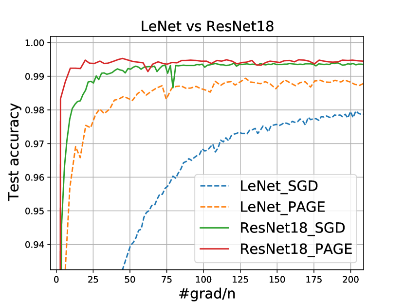
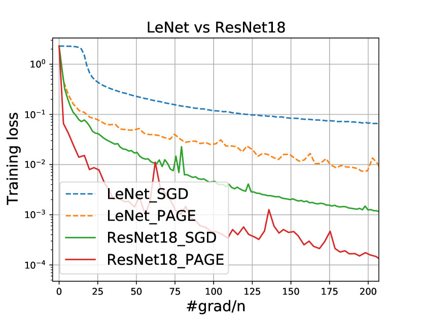
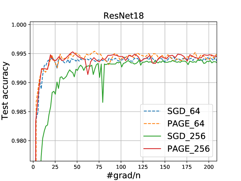
(1c) Different neural networks

Figure 1: LeNet and ResNet18 on MNIST dataset

Theorem 6 (Nonconvex online problem (3) under PL)

Suppose that Assumptions 1, 2 and 3 hold. Choose the stepsize $\eta\leq\min\{\frac{1}{L\left(1+\sqrt{\frac{1-p}{pb^{\prime}}}\right)},~{}\frac{p}{2\mu}\}$, minibatch size $b=\min\{\lceil\frac{2\sigma^{2}}{\mu\epsilon}\rceil,n\}$, secondary minibatch size $b^{\prime}<b$, and probability $p_{t}\equiv p\in(0,1]$. Then the number of iterations performed by PAGE sufficient for finding an $\epsilon$-solution (${\mathbb{E}}[f(x^{T})-f^{*}]\leq\epsilon$) of nonconvex finite-sum problem (2) can be bounded by

$$T=\left(\Big{(}1+\sqrt{\frac{1-p}{pb^{\prime}}}\Big{)}\kappa+\frac{2}{p}\right)\log\frac{2{\Delta_{0}}}{\epsilon}.$$

Moreover, the number of stochastic gradient computations (i.e., gradient complexity) $\#\mathrm{grad}=b+T\left(pb+(1-p)b^{\prime}\right)$ is

$$b+\left(pb+(1-p)b^{\prime}\right)\left(\Big{(}1+\sqrt{\frac{1-p}{pb^{\prime}}}\Big{)}\kappa+\frac{2}{p}\right)\log\frac{2{\Delta_{0}}}{\epsilon}.$$

Corollary 7

Suppose that Assumptions 1, 2 and 3 hold. Choose the stepsize $\eta\leq\min\{\frac{1}{L(1+\sqrt{b}/b^{\prime})},~{}\frac{b^{\prime}}{2\mu(b+b^{\prime})}\}$, minibatch size $b=\min\{\lceil\frac{2\sigma^{2}}{\mu\epsilon}\rceil,n\}$, secondary minibatch $b^{\prime}\leq\sqrt{b}$ and probability $p_{t}\equiv\frac{b^{\prime}}{b+b^{\prime}}$. Then the number of iterations performed by PAGE to find an $\epsilon$-solution of nonconvex online problem (3) can be bounded by $T=\left((1+\frac{\sqrt{b}}{b^{\prime}})\kappa+\frac{2(b+b^{\prime})}{b^{\prime}}\right)\log\frac{2{\Delta_{0}}}{\epsilon}.$ Moreover, the number of stochastic gradient computations (gradient complexity) is

$$\#\mathrm{grad}=O\left((b+\sqrt{b}\kappa)\log\frac{1}{\epsilon}\right).$$

6 Experiments

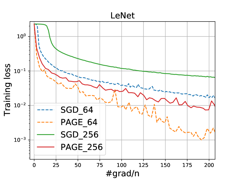
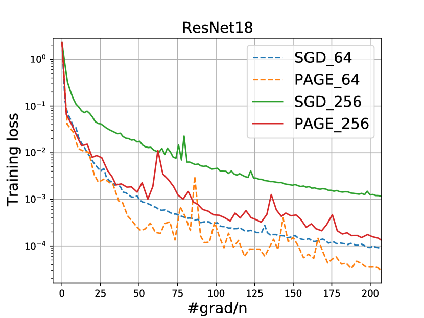
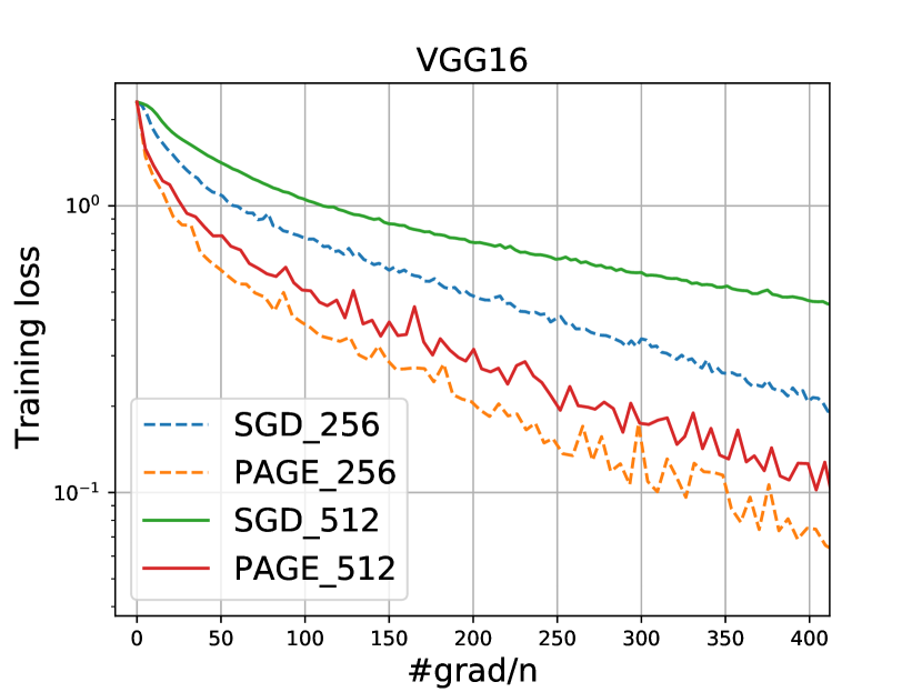
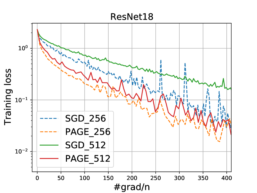
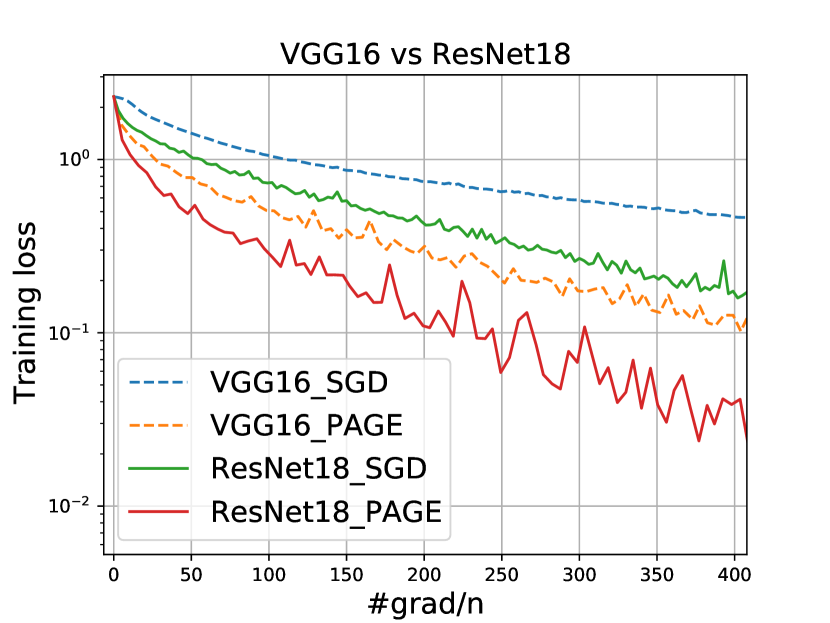
In this section, we conduct several deep learning experiments for multi-class image classification. Concretely, we compare our PAGE algorithm with vanilla SGD by running standard LeNet (LeCun et al., 1998), VGG (Simonyan & Zisserman, 2014) and ResNet (He et al., 2016) models on MNIST (LeCun et al., 1998) and CIFAR-10 (Krizhevsky, 2009) datasets. We implement the algorithms in PyTorch (Paszke et al., 2019) and run the experiments on several NVIDIA Tesla V100 GPUs.

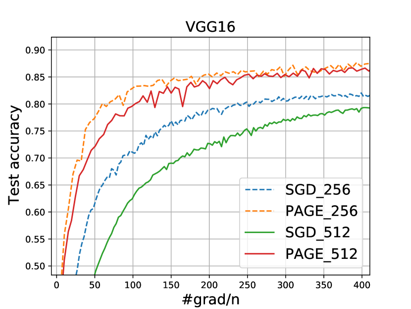
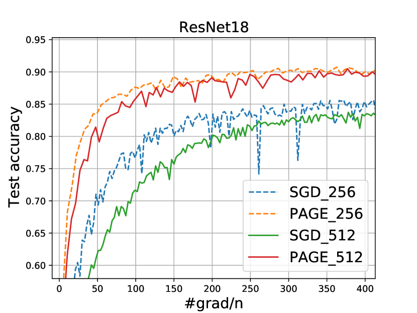
According to the update form in PAGE (see Line 4 of Algorithm 1), PAGE enjoys a lower computational cost than vanilla minibatch SGD (i.e., $p_{t}\equiv 1$ in PAGE) since $b^{\prime}<b$. Thus, in the experiments we want to show how the performance of PAGE compares with vanilla minibatch SGD under different minibatch sizes $b$ (i.e., $b=64,256,512$). Note that we do not tune the parameters for PAGE, i.e., we set $b^{\prime}=\sqrt{b}$ and $p_{t}\equiv\frac{b^{\prime}}{b+b^{\prime}}=\frac{\sqrt{b}}{b+\sqrt{b}}$ according to our theoretical results (see e.g., Corollary 2 and 4). For the stepsize/learning rate $\eta$, we choose the same one for both PAGE and minibatch SGD according to the theoretical results.

(2a) Different minibatch size $b$

(2b) Different minibatch size $b$

(2c) Different neural networks

Figure 2: VGG16 and ResNet18 on CIFAR-10 dataset

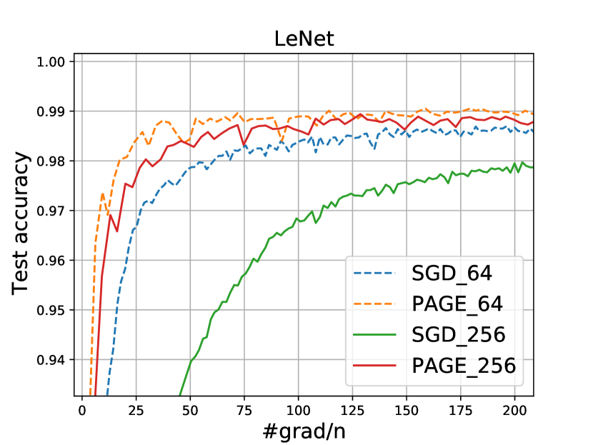
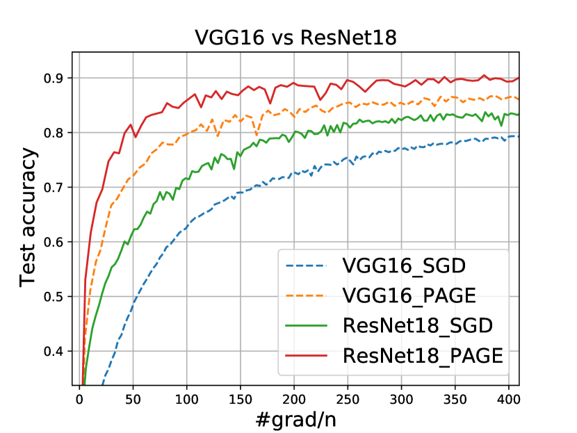
Concretely, in Figure 1, we choose standard minibatch $b=64$ and $b=256$ for both PAGE and vanilla minibatch SGD for MNIST experiments. In Figure 2, we choose $b=256$ and $b=512$ for CIFAR-10 experiments. The first row of Figures 1 and 2 denotes the training loss with respect to the gradient computations, and the second row denotes the test accuracy with respect to the gradient computations. Both Figures 1 and 2 demonstrate that PAGE not only converges much faster than SGD in training but also achieves higher test accuracy (which is typically very important in practice, e.g., lead to a better model). Moreover, the performance gap between PAGE and SGD is larger when the minibatch size $b$ is larger (i.e, gap between solid lines in Figures 1a, 1b, 2a, 2b), which is consistent with the update form of PAGE, i.e, it reuses the previous gradient with a small adjustment (lower computational cost $b^{\prime}=\sqrt{b}$ instead of $b$) with probability $1-p_{t}$. The experimental results validate our theoretical results and confirm the practical superiority of PAGE.

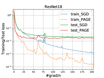
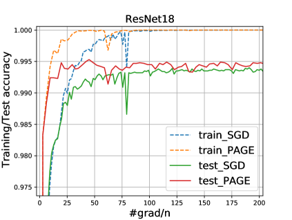
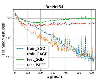
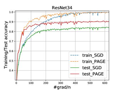
(3a) Training/test loss    (3b) Training/test accuracy

Figure 3: ResNet18 on MNIST dataset

In the following, we conduct extra experiments for comparing the training loss and test loss (Figure 3a, 4a), and training accuracy and test accuracy (Figure 3b, 4b) between PAGE and SGD. Note that Figure 3 (i.e., 3a, 3b) uses MNIST dataset and Figure 4 (i.e., 4a, 4b) uses CIFAR-10 dataset. Figures (3a) and (4a) also demonstrate that PAGE converges much faster than SGD both in training loss and test loss. Moreover, Figures (3b) and (4b) demonstrate that PAGE achieves the higher test accuracy than SGD and converges faster in training accuracy. Thus, our PAGE is not only converging faster than SGD in training but also achieves the higher test accuracy (which is typically very important in practice, e.g., lead to a better model). Again, the experimental results validate our theoretical results and confirm the practical superiority of PAGE.

(4a) Training/test loss    (4b) Training/test accuracy

Figure 4: ResNet34 on CIFAR-10 dataset

7 Conclusion

In this paper, we propose a simple and optimal PAGE algorithm for both nonconvex finite-sum and online optimization. We prove tight lower bounds and show that PAGE achieves the optimal convergence results matching our lower bounds for both nonconvex finite-sum problems and online problems. We also show that for nonconvex functions satisfying the PL condition, PAGE can automatically switch to a faster linear convergence rate. Besides, PAGE is easy to implement and we conduct several deep learning experiments (e.g., LeNet, VGG, ResNet) in PyTorch which confirm the practical superiority of PAGE. More importantly, the novel convergence analysis of PAGE is very simple and clean. Thus PAGE and its analysis can be easily adopted and generalized to other works. In fact, it already leads to some further breakthroughs in communication-efficient distributed learning (e.g., Gorbunov et al., 2021; Richtárik et al., 2021).

Appendix A Missing Proofs for Nonconvex Finite-Sum Problems

Appendix A and Appendix B provide proof details for nonconvex finite-sum and online problems, respectively. For the PL setting where faster linear convergence rates can be obtained, Appendix C and Appendix D provide proof details for nonconvex finite-sum and online problems under PL condition, respectively. Before providing the detailed proofs for main theorems and corollaries, we first provide a lemma of smoothness and a general key technical lemma which are used in the following Appendices A–D regardless of the settings.

Lemma 1

If function $f(x):=\frac{1}{n}\sum_{i=1}^{n}f_{i}(x)$ is average $L$-smooth (see Assumption 2), i.e., if

$${\mathbb{E}}_{i}[\|\nabla f_{i}(x)-\nabla f_{i}(y)\|^{2}]\leq L^{2}\|x-y\|^{2},\quad\forall x,y\in{\mathbb{R}}^{d},$$ (7)

then $f$ is also $L$-smooth, i.e., $\|\nabla f(x)-\nabla f(y)\|\leq L\|x-y\|$ and thus

$$f(y)\leq f(x)+\langle\nabla f(x),y-x\rangle+\frac{L}{2}\|y-x\|^{2},\quad\forall x,y\in{\mathbb{R}}^{d}.$$ (8)

Proof of Lemma 1. First, we show the $L$-smoothness of $f$:

$$\|\nabla f(x)-\nabla f(y)\| = \sqrt{\|{\mathbb{E}}_{i}[\nabla f_{i}(x)-\nabla f_{i}(y)]\|^{2}}$$ (9)

$$\leq \sqrt{{\mathbb{E}}_{i}[\|\nabla f_{i}(x)-\nabla f_{i}(y)\|^{2}]}$$

$$\overset{\eqref{eq:avg-smooth}}{\leq} \sqrt{L^{2}\|x-y\|^{2}}$$

$$= L\|x-y\|,$$

where the first inequality uses Jensen’s inequality: $g({\mathbb{E}}[x])\leq{\mathbb{E}}[g(x)]$ for a convex function $g$. Then, inequality (8) holds due to standard arguments (we do not claim any novelty here and include the following arguments for completeness):

$$f(y) = f(x)+\int_{0}^{1}\langle\nabla f(x+\tau(y-x)),y-x\rangle d\tau$$ (10)

$$= f(x)+\langle\nabla f(x),y-x\rangle+\int_{0}^{1}\langle\nabla f(x+\tau(y-x))-\nabla f(x),y-x\rangle d\tau$$

$$\leq f(x)+\langle\nabla f(x),y-x\rangle+\int_{0}^{1}\|\nabla f(x+\tau(y-x))-\nabla f(x)\|\|y-x\|d\tau$$

$$\overset{\eqref{eq:L-smooth}}{\leq} f(x)+\langle\nabla f(x),y-x\rangle+\int_{0}^{1}L\tau\|y-x\|^{2}d\tau$$

$$= f(x)+\langle\nabla f(x),y-x\rangle+\frac{L}{2}\|y-x\|^{2},$$

where the first inequality uses Cauchy–Schwarz inequality $\langle u,v\rangle\leq\|u\|\|v\|$. $\Box$

Now, we provide a key Lemma 2 which describes a useful relation between the function values after and before a gradient descent step, i.e., between $f(x^{t+1})$ and $f(x^{t})$ with $x^{t+1}:=x^{t}-\eta g^{t}$ for any gradient estimator $g^{t}\in{\mathbb{R}}^{d}$ and stepsize $\eta>0$.

Lemma 2

Suppose that function $f$ is $L$-smooth and let $x^{t+1}:=x^{t}-\eta g^{t}$. Then for any $g^{t}\in{\mathbb{R}}^{d}$ and $\eta>0$, we have

$$f(x^{t+1})\leq f(x^{t})-\frac{\eta}{2}\|\nabla f(x^{t})\|^{2}-\Big{(}\frac{1}{2\eta}-\frac{L}{2}\Big{)}\|x^{t+1}-x^{t}\|^{2}+\frac{\eta}{2}\|g^{t}-\nabla f(x^{t})\|^{2}.$$ (11)

Proof of Lemma 2. Let $\bar{x}^{t+1}:=x^{t}-\eta\nabla f(x^{t})$. In view of $L$-smoothness of $f$, we have

$$f(x^{t+1}) \overset{\eqref{eq:smooth}}{\leq} f(x^{t})+\langle\nabla f(x^{t}),x^{t+1}-x^{t}\rangle+\frac{L}{2}\|x^{t+1}-x^{t}\|^{2}$$

$$= f(x^{t})+\langle\nabla f(x^{t})-g^{t},x^{t+1}-x^{t}\rangle+\langle g^{t},x^{t+1}-x^{t}\rangle+\frac{L}{2}\|x^{t+1}-x^{t}\|^{2}$$

$$= f(x^{t})+\langle\nabla f(x^{t})-g^{t},-\eta g^{t}\rangle-\Big{(}\frac{1}{\eta}-\frac{L}{2}\Big{)}\|x^{t+1}-x^{t}\|^{2}$$

$$= f(x^{t})+\eta\|\nabla f(x^{t})-g^{t}\|^{2}-\eta\langle\nabla f(x^{t})-g^{t},\nabla f(x^{t})\rangle-\Big{(}\frac{1}{\eta}-\frac{L}{2}\Big{)}\|x^{t+1}-x^{t}\|^{2}$$

$$= f(x^{t})+\eta\|\nabla f(x^{t})-g^{t}\|^{2}-\frac{1}{\eta}\langle x^{t+1}-\bar{x}^{t+1},x^{t}-\bar{x}^{t+1}\rangle-\Big{(}\frac{1}{\eta}-\frac{L}{2}\Big{)}\|x^{t+1}-x^{t}\|^{2}$$

$$= f(x^{t})+\eta\|\nabla f(x^{t})-g^{t}\|^{2}-\Big{(}\frac{1}{\eta}-\frac{L}{2}\Big{)}\|x^{t+1}-x^{t}\|^{2}$$

$$\qquad\qquad\qquad-\frac{1}{2\eta}\Big{(}\|x^{t+1}-\bar{x}^{t+1}\|^{2}+\|x^{t}-\bar{x}^{t+1}\|^{2}-\|x^{t+1}-x^{t}\|^{2}\Big{)}$$

$$= f(x^{t})+\eta\|\nabla f(x^{t})-g^{t}\|^{2}-\Big{(}\frac{1}{\eta}-\frac{L}{2}\Big{)}\|x^{t+1}-x^{t}\|^{2}$$

$$\qquad\qquad\qquad-\frac{1}{2\eta}\Big{(}\eta^{2}\|\nabla f(x^{t})-g^{t}\|^{2}+\eta^{2}\|\nabla f(x^{t})\|^{2}-\|x^{t+1}-x^{t}\|^{2}\Big{)}$$

$$= f(x^{t})-\frac{\eta}{2}\|\nabla f(x^{t})\|^{2}-\Big{(}\frac{1}{2\eta}-\frac{L}{2}\Big{)}\|x^{t+1}-x^{t}\|^{2}+\frac{\eta}{2}\|g^{t}-\nabla f(x^{t})\|^{2}.$$

$\Box$

Now, we are ready to provide the detailed proofs for our main convergence theorem and corollaries for PAGE in the nonconvex finite-sum case (i.e., problem (2)).

A.1 Proof of Main Theorem 1

In this appendix, we first restate our main convergence result (Theorem 1) in the nonconvex finite-sum case and then provide its proof.

Theorem 1 (Main theorem for nonconvex finite-sum problem (2))

Suppose that Assumption 2 holds. Choose the stepsize

$$\eta\leq\frac{1}{L\left(1+\sqrt{\frac{1-p}{pb^{\prime}}}\right)},$$

minibatch size $b=n$, secondary minibatch size $b^{\prime}<b$, and probability $p_{t}\equiv p\in(0,1]$. Then the number of iterations performed by PAGE sufficient for finding an $\epsilon$-approximate solution (i.e., ${\mathbb{E}}[\|\nabla f(\widehat{x}_{T})\|]\leq\epsilon$) of nonconvex finite-sum problem (2) can be bounded by

$$T=\frac{2{\Delta_{0}}L}{\epsilon^{2}}\left(1+\sqrt{\frac{1-p}{pb^{\prime}}}\right).$$ (12)

Moreover, the number of stochastic gradient computations (i.e., gradient complexity) is

$$\#\mathrm{grad}=b+T\left(pb+(1-p)b^{\prime}\right)=b+\frac{2{\Delta_{0}}L}{\epsilon^{2}}\left(1+\sqrt{\frac{1-p}{pb^{\prime}}}\right)\left(pb+(1-p)b^{\prime}\right).$$ (13)

Note that the first $b$ in $\#\mathrm{grad}$ is due to the computation of $g^{0}$ (see Line 1 in Algorithm 1).

Proof of Theorem 1. Note that since the average $L$-smoothness assumption (Assumption 2) holds for $f$, we know that $f$ is also $L$-smooth according to Lemma 1. Then according to the update step $x^{t+1}:=x^{t}-\eta g^{t}$ (see Line 3 in Algorithm 1) and Lemma 2, we have

$$f(x^{t+1})\leq f(x^{t})-\frac{\eta}{2}\|\nabla f(x^{t})\|^{2}-\Big{(}\frac{1}{2\eta}-\frac{L}{2}\Big{)}\|x^{t+1}-x^{t}\|^{2}+\frac{\eta}{2}\|g^{t}-\nabla f(x^{t})\|^{2}.$$ (14)

Now, we use the following Lemma 3 to bound the last variance term of (14) for this finite-sum case.

Lemma 3

Suppose that Assumption 2 holds. If the gradient estimator $g^{t+1}$ is defined in Line 4 of Algorithm 1, then we have

$${\mathbb{E}}[\|g^{t+1}-\nabla f(x^{t+1})\|^{2}]\leq(1-p_{t})\|g^{t}-\nabla f(x^{t})\|^{2}+\frac{(1-p_{t})L^{2}}{b^{\prime}}\|x^{t+1}-x^{t}\|^{2}.$$ (15)

Proof of Lemma 3. According to the definition of PAGE gradient estimator in Line 4 of Algorithm 1:

$$g^{t+1}=\begin{cases}\frac{1}{b}\sum\limits_{i\in I}\nabla f_{i}(x^{t+1})&\text{with probability }p_{t},\\ g^{t}+\frac{1}{b^{\prime}}\sum\limits_{i\in I^{\prime}}(\nabla f_{i}(x^{t+1})-\nabla f_{i}(x^{t}))&\text{with probability }1-p_{t}.\end{cases}$$ (16)

A direct calculation now reveals that

$${\mathbb{E}}[\|g^{t+1}-\nabla f(x^{t+1})\|^{2}]$$

$$\overset{\eqref{eq:gt}}{=}p_{t}{\mathbb{E}}\left[\left\|\frac{1}{b}\sum_{i\in I}\nabla f_{i}(x^{t+1})-\nabla f(x^{t+1})\right\|^{2}\right]+(1-p_{t}){\mathbb{E}}\left[\left\|g^{t}+\frac{1}{b^{\prime}}\sum_{i\in I^{\prime}}(\nabla f_{i}(x^{t+1})-\nabla f_{i}(x^{t}))-\nabla f(x^{t+1})\right\|^{2}\right]$$

$$=(1-p_{t}){\mathbb{E}}\left[\left\|g^{t}+\frac{1}{b^{\prime}}\sum_{i\in I^{\prime}}(\nabla f_{i}(x^{t+1})-\nabla f_{i}(x^{t}))-\nabla f(x^{t+1})\right\|^{2}\right]$$ (17)

$$=(1-p_{t}){\mathbb{E}}\left[\left\|g^{t}-\nabla f(x^{t})+\frac{1}{b^{\prime}}\sum_{i\in I^{\prime}}(\nabla f_{i}(x^{t+1})-\nabla f_{i}(x^{t}))-\nabla f(x^{t+1})+\nabla f(x^{t})\right\|^{2}\right]$$

$$=(1-p_{t}){\mathbb{E}}\left[\left\|\frac{1}{b^{\prime}}\sum_{i\in I^{\prime}}(\nabla f_{i}(x^{t+1})-\nabla f_{i}(x^{t}))-\nabla f(x^{t+1})+\nabla f(x^{t})\right\|^{2}\right]+(1-p_{t})\|g^{t}-\nabla f(x^{t})\|^{2}$$

$$=\frac{1-p_{t}}{b^{\prime 2}}{\mathbb{E}}\left[\sum_{i\in I^{\prime}}\left\|\left(\nabla f_{i}(x^{t+1})-\nabla f_{i}(x^{t})\right)-\left(\nabla f(x^{t+1})-\nabla f(x^{t})\right)\right\|^{2}\right]+(1-p_{t})\|g^{t}-\nabla f(x^{t})\|^{2}$$

$$\leq\frac{1-p_{t}}{b^{\prime}}{\mathbb{E}}[\|\nabla f_{i}(x^{t+1})-\nabla f_{i}(x^{t})\|^{2}]+(1-p_{t})\|g^{t}-\nabla f(x^{t})\|^{2}$$

$$\leq\frac{(1-p_{t})L^{2}}{b^{\prime}}\|x^{t+1}-x^{t}\|^{2}+(1-p_{t})\|g^{t}-\nabla f(x^{t})\|^{2},$$ (18)

where (17) holds since we let $b=n$ in this finite-sum case, the last inequality (18) is due to the average $L$-smoothness Assumption 2 (i.e., (5)). $\Box$

Now, we continue to prove Theorem 1 using Lemma 3. We add (14) with $\frac{\eta}{2p}$ $\times$ (15) (here we simply let $p_{t}\equiv p$), and take expectation to get

$${\mathbb{E}}\left[f(x^{t+1})-f^{*}+\frac{\eta}{2p}\|g^{t+1}-\nabla f(x^{t+1})\|^{2}\right]$$

$$\leq{\mathbb{E}}\left[f(x^{t})-f^{*}-\frac{\eta}{2}\|\nabla f(x^{t})\|^{2}-\Big{(}\frac{1}{2\eta}-\frac{L}{2}\Big{)}\|x^{t+1}-x^{t}\|^{2}+\frac{\eta}{2}\|g^{t}-\nabla f(x^{t})\|^{2}\right]$$

$$\qquad+\frac{\eta}{2p}{\mathbb{E}}\left[(1-p)\|g^{t}-\nabla f(x^{t})\|^{2}+\frac{(1-p)L^{2}}{b^{\prime}}\|x^{t+1}-x^{t}\|^{2}\right]$$

$$={\mathbb{E}}\left[f(x^{t})-f^{*}+\frac{\eta}{2p}\|g^{t}-\nabla f(x^{t})\|^{2}-\frac{\eta}{2}\|\nabla f(x^{t})\|^{2}-\Big{(}\frac{1}{2\eta}-\frac{L}{2}-\frac{(1-p)\eta L^{2}}{2pb^{\prime}}\Big{)}\|x^{t+1}-x^{t}\|^{2}\right]$$

$$\leq{\mathbb{E}}\left[f(x^{t})-f^{*}+\frac{\eta}{2p}\|g^{t}-\nabla f(x^{t})\|^{2}-\frac{\eta}{2}\|\nabla f(x^{t})\|^{2}\right],$$ (19)

where the last inequality (19) holds due to $\frac{1}{2\eta}-\frac{L}{2}-\frac{(1-p)\eta L^{2}}{2pb^{\prime}}\geq 0$ by choosing stepsize

$$\eta\leq\frac{1}{L\left(1+\sqrt{\frac{1-p}{pb^{\prime}}}\right)}.$$ (20)

Now, if we define $\Phi_{t}:=f(x^{t})-f^{*}+\frac{\eta}{2p}\|g^{t}-\nabla f(x^{t})\|^{2}$, then (19) can be written in the form

$${\mathbb{E}}[\Phi_{t+1}]\leq{\mathbb{E}}[\Phi_{t}]-\frac{\eta}{2}{\mathbb{E}}[\|\nabla f(x^{t})\|^{2}].$$ (21)

Summing up from $t=0$ to $T-1$, we get

$${\mathbb{E}}[\Phi_{T}]\leq{\mathbb{E}}[\Phi_{0}]-\frac{\eta}{2}\sum_{t=0}^{T-1}{\mathbb{E}}[\|\nabla f(x^{t})\|^{2}].$$ (22)

Then according to the output of PAGE, i.e., $\widehat{x}_{T}$ is randomly chosen from $\{x^{t}\}_{t\in[T]}$ and $\Phi_{0}=f(x^{0})-f^{*}+\frac{\eta}{2p}\|g^{0}-\nabla f(x^{0})\|^{2}=f(x^{0})-f^{*}\overset{\text{def}}{=}{\Delta_{0}}$, we have

$${\mathbb{E}}[\|\nabla f(\widehat{x}_{T})\|^{2}]\leq\frac{2{\Delta_{0}}}{\eta T}.$$ (23)

If we set the number of iterations as

$$T=\frac{2{\Delta_{0}}}{\epsilon^{2}\eta}\overset{\eqref{eq:eta}}{=}\frac{2{\Delta_{0}}L}{\epsilon^{2}}\left(1+\sqrt{\frac{1-p}{pb^{\prime}}}\right),$$ (24)

then (23) and Jensen’s inequality imply

$${\mathbb{E}}[\|\nabla f(\widehat{x}_{T})\|]\leq\sqrt{{\mathbb{E}}[\|\nabla f(\widehat{x}_{T})\|^{2}]}\leq\sqrt{\frac{2{\Delta_{0}}}{\eta T}}=\epsilon.$$

$\Box$

A.2 Proofs of Corollaries 1 and 2

Similarly, we first restate the corollaries and then provide their proofs respectively.

Corollary 1 (We recover GD by letting $p_{t}\equiv 1$)

Suppose that Assumption 2 holds. Choose the stepsize $\eta\leq\frac{1}{L}$, minibatch size $b=n$ and probability $p_{t}\equiv 1$. Then PAGE reduces to GD, and the number of iterations performed by PAGE to find an $\epsilon$-approximate solution of the nonconvex finite-sum problem (2) can be bounded by $T=\frac{2{\Delta_{0}}L}{\epsilon^{2}}.$ Moreover, the number of stochastic gradient computations (i.e., gradient complexity) is

$$\#\mathrm{grad}=n+\frac{2{\Delta_{0}}Ln}{\epsilon^{2}}=O\left(\frac{n}{\epsilon^{2}}\right).$$ (25)

Proof of Corollary 1. If the probability is set to $p=1$, the term $\sqrt{\frac{1-p}{pb^{\prime}}}$ disappears from the stepsize $\eta$, and the total number of iterations $T$ in Theorem 1. So, the bound on the stepsize simplified to $\eta\leq\frac{1}{L}$, and the total number of iterations simplifies to $T=\frac{2{\Delta_{0}}L}{\epsilon^{2}}$. We know that the gradient estimator of PAGE (Line 4 of Algorithm 1) uses $pb+(1-p)b^{\prime}=b$ stochastic gradients in each iteration. Thus, the gradient complexity is $\#\mathrm{grad}=b+Tb=n+\frac{2{\Delta_{0}}Ln}{\epsilon^{2}}$, as claimed. $\Box$

Corollary 2 (Optimal result for nonconvex finite-sum problem (2))

Suppose that Assumption 2 holds. Choose the stepsize $\eta\leq\frac{1}{L(1+\sqrt{b}/b^{\prime})}$, minibatch size $b=n$, secondary minibatch size $b^{\prime}\leq\sqrt{b}$ and probability $p_{t}\equiv\frac{b^{\prime}}{b+b^{\prime}}$. Then the number of iterations performed by PAGE to find an $\epsilon$-approximate solution of the nonconvex finite-sum problem (2) can be bounded by $T=\frac{2{\Delta_{0}}L}{\epsilon^{2}}(1+\frac{\sqrt{b}}{b^{\prime}}).$ Moreover, the number of stochastic gradient computations (i.e., gradient complexity) is

$$\#\mathrm{grad}\leq n+\frac{8{\Delta_{0}}L\sqrt{n}}{\epsilon^{2}}=O\left(n+\frac{\sqrt{n}}{\epsilon^{2}}\right).$$ (26)

Proof of Corollary 2. If we choose probability $p=\frac{b^{\prime}}{b+b^{\prime}}$, then $\sqrt{\frac{1-p}{pb^{\prime}}}=\frac{\sqrt{b}}{b^{\prime}}$. Thus, according to Theorem 1, the stepsize bound becomes $\eta\leq\frac{1}{L(1+\sqrt{b}/b^{\prime})}$ and the total number of iterations becomes $T=\frac{2{\Delta_{0}}L}{\epsilon^{2}}(1+\frac{\sqrt{b}}{b^{\prime}})$. We know that the gradient estimator of PAGE (Line 4 of Algorithm 1) uses $pb+(1-p)b^{\prime}=\frac{2bb^{\prime}}{b+b^{\prime}}$ stochastic gradients in each iteration on expectation. Thus, the gradient complexity is

$$\#\mathrm{grad} =b+T\left(pb+(1-p)b^{\prime}\right)$$

$$=b+\frac{2{\Delta_{0}}L}{\epsilon^{2}}\left(1+\frac{\sqrt{b}}{b^{\prime}}\right)\frac{2bb^{\prime}}{b+b^{\prime}}$$

$$\leq b+\frac{2{\Delta_{0}}L}{\epsilon^{2}}\left(1+\frac{\sqrt{b}}{b^{\prime}}\right)2b^{\prime}$$

$$\leq n+\frac{8{\Delta_{0}}L\sqrt{n}}{\epsilon^{2}},$$

where the last inequality is due to the parameter setting $b=n$ and $b^{\prime}\leq\sqrt{b}$. $\Box$

A.3 Proof of Theorem 2

Before providing the proof for the lower bound theorem, we recall the standard definition of the algorithm class of linear-span first-order algorithms.

Definition 1 (Linear-span first-order algorithm)

Consider a (randomized) algorithm ${\mathcal{A}}$ starting with $x^{0}$ and let $x^{t}$ be the point obtained at iteration $t\geq 0$. Then ${\mathcal{A}}$ is called a linear-span first-order algorithm if

$$x^{t}\in\mathrm{Lin}\{x^{0},x^{1},\ldots,x^{t-1},\nabla f_{i_{0}}(x^{0}),\nabla f_{i_{1}}(x^{1}),\ldots,\nabla f_{i_{t-1}}(x^{t-1})\},$$ (27)

where Lin denotes the linear span, and $i_{j}$ denotes the individual function (or multiple functions) chosen by ${\mathcal{A}}$ at iteration $j$.

We now restate the lower bound result (Theorem 2) and then provide its proof.

Theorem 2 (Lower bound)

For any $L>0$, ${\Delta_{0}}>0$ and $n>0$, there exists a large enough dimension $d$ and a function $f:{\mathbb{R}}^{d}\to{\mathbb{R}}$ satisfying Assumption 2 in the finite-sum case such that any linear-span first-order algorithm needs $\Omega(n+\frac{{\Delta_{0}}L\sqrt{n}}{\epsilon^{2}})$ stochastic gradient computations in order to finding an $\epsilon$-approximate solution, i.e., a point $\widehat{x}$ such that ${\mathbb{E}}\|\nabla f(\widehat{x})\|\leq\epsilon$.

Proof of Theorem 2. Consider the function $f(x)=\frac{1}{n}\sum_{i=1}^{n}f_{i}(x)$, where

$$f_{i}(x):=c\langle v_{i},x\rangle+\frac{L}{2}\|x\|^{2}$$ (28)

for some constant $c$. First, we show that $f:{\mathbb{R}}^{d}\to{\mathbb{R}}$ satisfies Assumption 2 as follows:

$${\mathbb{E}}_{i}[\|\nabla f_{i}(x)-\nabla f_{i}(y)\|^{2}] ={\mathbb{E}}_{i}[\|(cv_{i}+Lx)-(cv_{i}+Ly)\|^{2}]$$

$$={\mathbb{E}}_{i}[\|L(x-y)\|^{2}]$$

$$=L^{2}\|x-y\|^{2}.$$

Without loss of generality, we assume that $x^{0}=0$. Otherwise one can consider the shifted function $f(x+x^{0})$ instead. Now, we compute ${\Delta_{0}}$ as follows:

$$f(x^{0})-f^{*} =f(0)-f(x^{*})$$

$$=0-\left(\frac{c}{n}\sum_{i=1}^{n}\langle v_{i},x^{*}\rangle+\frac{L}{2}\|x^{*}\|^{2}\right)$$

$$=\frac{c^{2}}{2Ln^{2}}\bigg{\|}\sum_{i=1}^{n}v_{i}\bigg{\|}^{2}$$ (29)

$$={\Delta_{0}},$$ (30)

where the equality (29) is due to $x^{*}=-\frac{c}{Ln}\sum_{i=1}^{n}v_{i}$, and the last equality holds by choosing the appropriate parameter $c$. Note that we only need to consider the case $\epsilon\leq O(\sqrt{{\Delta_{0}}L})$ since the gradient norm at the initial point $x^{0}$ already achieves this order, i.e., $\|\nabla f(x^{0})\|\leq\sqrt{2{\Delta_{0}}L}$. Indeed, since

$$f^{*} \leq f\left(x^{0}-\frac{1}{L}\nabla f(x^{0})\right)$$

$$\leq f(x^{0})+\left\langle\nabla f(x^{0}),-\frac{1}{L}\nabla f(x^{0})\right\rangle+\frac{L}{2}\left\|\frac{1}{L}\nabla f(x^{0})\right\|^{2}$$ (31)

$$=f(x^{0})-\frac{1}{2L}\|\nabla f(x^{0})\|^{2},$$

where the inequality (31) uses the $L$-smoothness of $f$ (see Lemma 1), we have $\|\nabla f(x^{0})\|\leq\sqrt{2L(f(x^{0})-f^{*})}=\sqrt{2{\Delta_{0}}L}$.

Now according to the definition of linear-span first-order algorithms (i.e., Definition 1) and noting that the stochastic gradient is $\nabla f_{i}(x)=cv_{i}+Lx$ and $x^{0}=0$, after querying $t$ stochastic gradients, we have

$$x^{t}\in\mathrm{Lin}\{v_{i_{0}},v_{i_{1}},\ldots,v_{i_{t-1}}\},$$ (32)

where $i_{0},i_{1},\ldots,i_{t-1}$ denote the $t$ functions which are queried for stochastic gradient computations. For the gradient norm, we have

$$\|\nabla f(x)\|=\bigg{\|}\frac{c}{n}\sum_{i=1}^{n}v_{i}+Lx\bigg{\|}.$$ (33)

If we choose $\{v_{i}\}_{i\in[n]}$ to be orthogonal vectors, for example, choose $v_{1}=(1,1,\ldots,1,0,\ldots,0)^{T}$ (the first $\frac{d}{n}$ elements are 1 and all remaining are 0), $v_{2}=(0,0,\ldots,0,1,1,\ldots,1,0,\ldots,0)^{T}$ (the elements with indices from $\frac{d}{n}+1$ to $\frac{2d}{n}$ are 1 and others are 0), $\ldots$, $v_{i}$ (the elements with indices from $\frac{(i-1)d}{n}+1$ to $\frac{id}{n}$ are 1 and others are 0). In other words, we divide the indices $\{1,2,\ldots,d\}$ into $n$ parts, and set one part to be 1 and other parts to be 0 for each $v_{i}$. Note that $v_{i}\in{\mathbb{R}}^{d}$, for all $i\in[n]$. Thus, if fewer than $\frac{n}{2}$ functions have been queried for stochastic gradient computations, then according to (32) we know that the current point $x$ belongs to a subspace with dimension at most $\frac{d}{n}\times\frac{n}{2}=\frac{d}{2}$ in ${\mathbb{R}}^{d}$. Moreover, according to (33) we have

$$\|\nabla f(x)\|\geq\frac{c}{n}\sqrt{\frac{d}{2}}=\Omega(\epsilon),$$ (34)

where the last equality holds by choosing appropriate parameters $c$ and $d$.

So far, we have shown a lower bound of $\Omega(n)$ stochastic gradient computations for any linear-span first-order algorithm finding an $\epsilon$-approximate solution. For the second term $\Omega(\frac{{\Delta_{0}}L\sqrt{n}}{\epsilon^{2}})$, we directly use the previous lower bound provided by Fang et al. (2018). They proved this lower bound term in the small $n$ case, i.e., $n\leq O(\frac{{\Delta_{0}}^{2}L^{2}}{\epsilon^{4}})$. Here we recall their lower bound theorem.

Theorem 7 (Fang et al., 2018)

For any $L>0$, ${\Delta_{0}}>0$ and $n\leq O(\frac{{\Delta_{0}}^{2}L^{2}}{\epsilon^{4}})$, there exists a large enough dimension $d$ and a function $f:{\mathbb{R}}^{d}\to{\mathbb{R}}$ satisfying Assumption 2 in the finite-sum case such that any linear-span first-order algorithm needs $\Omega(\frac{{\Delta_{0}}L\sqrt{n}}{\epsilon^{2}})$ stochastic gradient computations in order to finding an $\epsilon$-approximate solution, i.e., a point $\widehat{x}$ such that ${\mathbb{E}}\|\nabla f(\widehat{x})\|\leq\epsilon$.

Now, the lower bound $\Omega(n+\frac{{\Delta_{0}}L\sqrt{n}}{\epsilon^{2}})$ is proved by combining the term $\Omega(\frac{{\Delta_{0}}L\sqrt{n}}{\epsilon^{2}})$ in the above theorem and $\Omega(n)$ in our previous arguments. $\Box$

Appendix B Missing Proofs for Nonconvex Online Problems

In this appendix, we provide the detailed proofs for our main convergence theorem and its corollaries for PAGE in the nonconvex online case (i.e., problem (3)). Recall that we refer this online problem (3) as the finite-sum problem (2) with large or infinite $n$. Also, we need the bounded variance assumption (Assumption 1) in this online case.

B.1 Proof of Main Theorem 3

Similarly to Appendix A.1, we first restate the main convergence result (Theorem 3) in the nonconvex online case and then provide its proof.

Theorem 3 (Main theorem for nonconvex online problem (3))

Suppose that Assumptions 1 and 2 hold. Choose the stepsize

$$\eta\leq\frac{1}{L\left(1+\sqrt{\frac{1-p}{pb^{\prime}}}\right)},$$

minibatch size $b=\min\{\lceil\frac{2\sigma^{2}}{\epsilon^{2}}\rceil,n\}$, secondary minibatch size $b^{\prime}<b$ and probability $p_{t}\equiv p\in(0,1]$. Then the number of iterations performed by PAGE to find an $\epsilon$-approximate solution (${\mathbb{E}}[\|\nabla f(\hat{x}_{T})\|]\leq\epsilon$) of nonconvex online problem (3) can be bounded by

$$T=\frac{4{\Delta_{0}}L}{\epsilon^{2}}\left(1+\sqrt{\frac{1-p}{pb^{\prime}}}\right)+\frac{1}{p}.$$ (35)

Moreover, the number of stochastic gradient computations (gradient complexity) is

$$\#\mathrm{grad}=b+T\left(pb+(1-p)b^{\prime}\right)=2b+\frac{(1-p)b^{\prime}}{p}+\frac{4{\Delta_{0}}L}{\epsilon^{2}}\left(1+\sqrt{\frac{1-p}{pb^{\prime}}}\right)\left(pb+(1-p)b^{\prime}\right).$$ (36)

Proof of Theorem 3. Similarly, we know that $f$ is also $L$-smooth according to Lemma 1. Then according to the update step $x^{t+1}:=x^{t}-\eta g^{t}$ (see Line 3 in Algorithm 1) and Lemma 2, we have

$$f(x^{t+1})\leq f(x^{t})-\frac{\eta}{2}\|\nabla f(x^{t})\|^{2}-\Big{(}\frac{1}{2\eta}-\frac{L}{2}\Big{)}\|x^{t+1}-x^{t}\|^{2}+\frac{\eta}{2}\|g^{t}-\nabla f(x^{t})\|^{2}.$$ (37)

Now, we use the following Lemma 4 to bound the last variance term of (37) for this online case.

Lemma 4

Suppose that Assumptions 1 and 2 hold. If the gradient estimator $g^{t+1}$ is defined in Line 4 of Algorithm 1, then we have

$${\mathbb{E}}[\|g^{t+1}-\nabla f(x^{t+1})\|^{2}]\leq(1-p_{t})\|g^{t}-\nabla f(x^{t})\|^{2}+\frac{(1-p_{t})L^{2}}{b^{\prime}}\|x^{t+1}-x^{t}\|^{2}+{\bf 1}_{\{b<n\}}\frac{p_{t}\sigma^{2}}{b}.$$ (38)

Proof of Lemma 4. According to the definition of PAGE gradient estimator in Line 4 of Algorithm 1

$$g^{t+1}=\begin{cases}\frac{1}{b}\sum\limits_{i\in I}\nabla f_{i}(x^{t+1})&\text{with probability }p_{t},\\ g^{t}+\frac{1}{b^{\prime}}\sum\limits_{i\in I^{\prime}}(\nabla f_{i}(x^{t+1})-\nabla f_{i}(x^{t}))&\text{with probability }1-p_{t},\end{cases}$$ (39)

we have

$${\mathbb{E}}[\|g^{t+1}-\nabla f(x^{t+1})\|^{2}]$$

$$\overset{\eqref{eq:gt-online}}{=}p_{t}{\mathbb{E}}\left[\left\|\frac{1}{b}\sum_{i\in I}\nabla f_{i}(x^{t+1})-\nabla f(x^{t+1})\right\|^{2}\right]+(1-p_{t}){\mathbb{E}}\left[\left\|g^{t}+\frac{1}{b^{\prime}}\sum_{i\in I^{\prime}}(\nabla f_{i}(x^{t+1})-\nabla f_{i}(x^{t}))-\nabla f(x^{t+1})\right\|^{2}\right]$$

$$={\bf 1}_{\{b<n\}}\frac{p_{t}\sigma^{2}}{b}+(1-p_{t}){\mathbb{E}}\left[\left\|g^{t}+\frac{1}{b^{\prime}}\sum_{i\in I^{\prime}}(\nabla f_{i}(x^{t+1})-\nabla f_{i}(x^{t}))-\nabla f(x^{t+1})\right\|^{2}\right]$$ (40)

$$={\bf 1}_{\{b<n\}}\frac{p_{t}\sigma^{2}}{b}+(1-p_{t}){\mathbb{E}}\left[\left\|g^{t}-\nabla f(x^{t})+\frac{1}{b^{\prime}}\sum_{i\in I^{\prime}}(\nabla f_{i}(x^{t+1})-\nabla f_{i}(x^{t}))-\nabla f(x^{t+1})+\nabla f(x^{t})\right\|^{2}\right]$$

$$={\bf 1}_{\{b<n\}}\frac{p_{t}\sigma^{2}}{b}+(1-p_{t})\|g^{t}-\nabla f(x^{t})\|^{2}+(1-p_{t}){\mathbb{E}}\left[\left\|\frac{1}{b^{\prime}}\sum_{i\in I^{\prime}}(\nabla f_{i}(x^{t+1})-\nabla f_{i}(x^{t}))-\nabla f(x^{t+1})+\nabla f(x^{t})\right\|^{2}\right]$$

$$={\bf 1}_{\{b<n\}}\frac{p_{t}\sigma^{2}}{b}+(1-p_{t})\|g^{t}-\nabla f(x^{t})\|^{2}+\frac{1-p_{t}}{b^{\prime 2}}{\mathbb{E}}\left[\sum_{i\in I^{\prime}}\left\|\left(\nabla f_{i}(x^{t+1})-\nabla f_{i}(x^{t})\right)-\left(\nabla f(x^{t+1})-\nabla f(x^{t})\right)\right\|^{2}\right]$$

$$\leq{\bf 1}_{\{b<n\}}\frac{p_{t}\sigma^{2}}{b}+(1-p_{t})\|g^{t}-\nabla f(x^{t})\|^{2}+\frac{1-p_{t}}{b^{\prime}}{\mathbb{E}}[\|\nabla f_{i}(x^{t+1})-\nabla f_{i}(x^{t})\|^{2}]$$

$$\leq{\bf 1}_{\{b<n\}}\frac{p_{t}\sigma^{2}}{b}+(1-p_{t})\|g^{t}-\nabla f(x^{t})\|^{2}+\frac{(1-p_{t})L^{2}}{b^{\prime}}\|x^{t+1}-x^{t}\|^{2},$$ (41)

where (40) is due to Assumption 1, i.e., (4) (where ${\bf 1_{\{\cdot\}}}$ denotes the indicator function), the last inequality (41) is due to the average $L$-smoothness Assumption 2, i.e., (5). $\Box$

Now, we continue to prove Theorem 3 using Lemma 4. We add (37) with $\frac{\eta}{2p}$ $\times$ (38) (here we simply let $p_{t}\equiv p$), and take expectation to get

$${\mathbb{E}}\left[f(x^{t+1})-f^{*}+\frac{\eta}{2p}\|g^{t+1}-\nabla f(x^{t+1})\|^{2}\right]$$

$$\leq{\mathbb{E}}\left[f(x^{t})-f^{*}-\frac{\eta}{2}\|\nabla f(x^{t})\|^{2}-\Big{(}\frac{1}{2\eta}-\frac{L}{2}\Big{)}\|x^{t+1}-x^{t}\|^{2}+\frac{\eta}{2}\|g^{t}-\nabla f(x^{t})\|^{2}\right]$$

$$\qquad+\frac{\eta}{2p}{\mathbb{E}}\left[(1-p)\|g^{t}-\nabla f(x^{t})\|^{2}+\frac{(1-p)L^{2}}{b^{\prime}}\|x^{t+1}-x^{t}\|^{2}+{\bf 1}_{\{b<n\}}\frac{p\sigma^{2}}{b}\right]$$

$$={\mathbb{E}}\Big{[}f(x^{t})-f^{*}+\frac{\eta}{2p}\|g^{t}-\nabla f(x^{t})\|^{2}-\frac{\eta}{2}\|\nabla f(x^{t})\|^{2}+{\bf 1}_{\{b<n\}}\frac{\eta\sigma^{2}}{2b}$$

$$\qquad-\Big{(}\frac{1}{2\eta}-\frac{L}{2}-\frac{(1-p)\eta L^{2}}{2pb^{\prime}}\Big{)}\|x^{t+1}-x^{t}\|^{2}\Big{]}$$

$$\leq{\mathbb{E}}\left[f(x^{t})-f^{*}+\frac{\eta}{2p}\|g^{t}-\nabla f(x^{t})\|^{2}-\frac{\eta}{2}\|\nabla f(x^{t})\|^{2}+{\bf 1}_{\{b<n\}}\frac{\eta\sigma^{2}}{2b}\right],$$ (42)

where the last inequality (42) holds due to $\frac{1}{2\eta}-\frac{L}{2}-\frac{(1-p)\eta L^{2}}{2pb^{\prime}}\geq 0$ by choosing stepsize

$$\eta\leq\frac{1}{L\left(1+\sqrt{\frac{1-p}{pb^{\prime}}}\right)}.$$ (43)

Now, if we define $\Phi_{t}:=f(x^{t})-f^{*}+\frac{\eta}{2p}\|g^{t}-\nabla f(x^{t})\|^{2}$, then (42) turns to

$${\mathbb{E}}[\Phi_{t+1}]\leq{\mathbb{E}}[\Phi_{t}]-\frac{\eta}{2}{\mathbb{E}}[\|\nabla f(x^{t})\|^{2}]+{\bf 1}_{\{b<n\}}\frac{\eta\sigma^{2}}{2b}.$$ (44)

Summing up it from $t=0$ for $T-1$, we have

$${\mathbb{E}}[\Phi_{T}]\leq{\mathbb{E}}[\Phi_{0}]-\frac{\eta}{2}\sum_{t=0}^{T-1}{\mathbb{E}}[\|\nabla f(x^{t})\|^{2}]+{\bf 1}_{\{b<n\}}\frac{\eta T\sigma^{2}}{2b}.$$ (45)

Then, according to the output of PAGE, i.e., $\widehat{x}_{T}$ is randomly chosen from $\{x^{t}\}_{t\in[T]}$, we have

$${\mathbb{E}}[\|\nabla f(\widehat{x}_{T})\|^{2}] \leq\frac{2{\mathbb{E}}[\Phi_{0}]}{\eta T}+{\bf 1}_{\{b<n\}}\frac{\sigma^{2}}{b}.$$ (46)

For the term ${\mathbb{E}}[\Phi_{0}]$, we have

$${\mathbb{E}}[\Phi_{0}] :={\mathbb{E}}\left[f(x^{0})-f^{*}+\frac{\eta}{2p}\|g^{0}-\nabla f(x^{0})\|^{2}\right]$$

$$={\mathbb{E}}\left[f(x^{0})-f^{*}+\frac{\eta}{2p}\left\|\frac{1}{b}\sum_{i\in I}\nabla f_{i}(x^{0})-\nabla f(x^{0})\right\|^{2}\right]$$ (47)

$$\leq f(x^{0})-f^{*}+{\bf 1}_{\{b<n\}}\frac{\eta\sigma^{2}}{2pb},$$ (48)

where (47) follows from the definition of $g^{0}$ (see Line 1 of Algorithm 1), and (48) is due to Assumption 1, i.e., (4) (where ${\bf 1_{\{\cdot\}}}$ denotes the indicator function). Plugging (48) into (46) and noting that ${\Delta_{0}}:=f(x^{0})-f^{*}$, we have

$${\mathbb{E}}[\|\nabla f(\widehat{x}_{T})\|^{2}] \leq\frac{2{\Delta_{0}}}{\eta T}+{\bf 1}_{\{b<n\}}\frac{\sigma^{2}}{pbT}+{\bf 1}_{\{b<n\}}\frac{\sigma^{2}}{b}$$

$$\leq\frac{2{\Delta_{0}}}{\eta T}+\frac{\epsilon^{2}}{2pT}+\frac{\epsilon^{2}}{2}$$ (49)

$$=\epsilon^{2},$$ (50)

where (49) follows from the parameter setting of minibatch size $b=\min\{\lceil\frac{2\sigma^{2}}{\epsilon^{2}}\rceil,n\}$, and the last equality (50) holds by letting the number of iterations

$$T=\frac{4{\Delta_{0}}}{\epsilon^{2}\eta}+\frac{1}{p}\overset{\eqref{eq:eta-online}}{=}\frac{4{\Delta_{0}}L}{\epsilon^{2}}\left(1+\sqrt{\frac{1-p}{pb^{\prime}}}\right)+\frac{1}{p}.$$ (51)

Now, the proof is finished since

$${\mathbb{E}}[\|\nabla f(\widehat{x}_{T})\|]\leq\sqrt{{\mathbb{E}}[\|\nabla f(\widehat{x}_{T})\|^{2}]} =\epsilon.$$ (52)

$\Box$

B.2 Proofs of Corollaries 3, 4 and 5

Similarly to Appendix A.2, we first restate the corollaries in this online case and then provide their proofs, respectively.

Corollary 3 (We recover SGD by letting $p_{t}\equiv 1$)

Suppose that Assumptions 1 and 2 hold. Let stepsize $\eta\leq\frac{1}{L}$, minibatch size $b=\lceil\frac{2\sigma^{2}}{\epsilon^{2}}\rceil$ and probability $p_{t}\equiv 1$, then the number of iterations performed by PAGE to find an $\epsilon$-approximate solution of nonconvex online problem (3) can be bounded by $T=\frac{4{\Delta_{0}}L}{\epsilon^{2}}+1.$ Moreover, the number of stochastic gradient computations (gradient complexity) is

$$\#\mathrm{grad}=\frac{4\sigma^{2}}{\epsilon^{2}}+\frac{8{\Delta_{0}}L\sigma^{2}}{\epsilon^{4}}=O\left(\frac{\sigma^{2}}{\epsilon^{4}}\right).$$ (53)

Proof of Corollary 3. If the probability parameter is set to $p=1$, then $\sqrt{\frac{1-p}{pb^{\prime}}}$ disappears from the stepsize $\eta$, and the total number of iterations $T$ in Theorem 3. Hence, the stepsize rule simplifies to $\eta\leq\frac{1}{L}$, and the total number of iterations becomes $T=\frac{4{\Delta_{0}}L}{\epsilon^{2}}+1$. We know that the gradient estimator of PAGE (Line 4 uses $pb+(1-p)b^{\prime}=b$ stochastic gradients in each iteration. Thus, the gradient complexity is $\#\mathrm{grad}=b+Tb=\frac{4\sigma^{2}}{\epsilon^{2}}+\frac{8{\Delta_{0}}L\sigma^{2}}{\epsilon^{4}}$. $\Box$

Corollary 4 (Optimal result for nonconvex online problem (3))

Suppose that Assumptions 1 and 2 hold. Choose the stepsize $\eta\leq\frac{1}{L(1+\sqrt{b}/b^{\prime})}$, minibatch size $b=\min\{\lceil\frac{2\sigma^{2}}{\epsilon^{2}}\rceil,n\}$, secondary minibatch size $b^{\prime}\leq\sqrt{b}$ and probability $p_{t}\equiv\frac{b^{\prime}}{b+b^{\prime}}$. Then the number of iterations performed by PAGE sufficient to find an $\epsilon$-approximate solution of nonconvex online problem (3) can be bounded by $T=\frac{4{\Delta_{0}}L}{\epsilon^{2}}(1+\frac{\sqrt{b}}{b^{\prime}})+\frac{b+b^{\prime}}{b^{\prime}}.$ Moreover, the number of stochastic gradient computations (i.e., gradient complexity) is

$$\#\mathrm{grad}\leq 3b+\frac{16{\Delta_{0}}L\sqrt{b}}{\epsilon^{2}}=O\left(b+\frac{\sqrt{b}}{\epsilon^{2}}\right).$$ (54)

Proof of Corollary 4. If we choose probability $p=\frac{b^{\prime}}{b+b^{\prime}}$, then $\sqrt{\frac{1-p}{pb^{\prime}}}=\frac{\sqrt{b}}{b^{\prime}}$. Thus, according to Theorem 3, the stepsize bound becomes $\eta\leq\frac{1}{L(1+\sqrt{b}/b^{\prime})}$ and the total number of iterations becomes $T=\frac{4{\Delta_{0}}L}{\epsilon^{2}}(1+\frac{\sqrt{b}}{b^{\prime}})+\frac{b+b^{\prime}}{b^{\prime}}$. Since the gradient estimator of PAGE (Line 4 of Algorithm 1) uses $pb+(1-p)b^{\prime}=\frac{2bb^{\prime}}{b+b^{\prime}}$ stochastic gradients in each iteration in expectation, the gradient complexity is

$$\#\mathrm{grad} =b+T\left(pb+(1-p)b^{\prime}\right)$$

$$=b+\left(\frac{4{\Delta_{0}}L}{\epsilon^{2}}\Big{(}1+\frac{\sqrt{b}}{b^{\prime}}\Big{)}+\frac{b+b^{\prime}}{b^{\prime}}\right)\frac{2bb^{\prime}}{b+b^{\prime}}$$

$$=3b+\frac{4{\Delta_{0}}L}{\epsilon^{2}}\Big{(}1+\frac{\sqrt{b}}{b^{\prime}}\Big{)}\frac{2bb^{\prime}}{b+b^{\prime}}$$

$$\leq 3b+\frac{4{\Delta_{0}}L}{\epsilon^{2}}\Big{(}1+\frac{\sqrt{b}}{b^{\prime}}\Big{)}2b^{\prime}$$

$$\leq 3b+\frac{16{\Delta_{0}}L\sqrt{b}}{\epsilon^{2}},$$

where the last inequality is due to the parameter setting $b^{\prime}\leq\sqrt{b}$. $\Box$

Corollary 5 (Lower bound)

For any $L>0$, ${\Delta_{0}}>0$, $\sigma^{2}>0$ and $n>0$, there exists a large enough dimension $d$ and a function $f:{\mathbb{R}}^{d}\to{\mathbb{R}}$ satisfying Assumptions 1 and 2 in the online case (here $n$ may be finite) such that any linear-span first-order algorithm needs $\Omega(b+\frac{{\Delta_{0}}L\sqrt{b}}{\epsilon^{2}})$, where $b=\min\{\frac{\sigma^{2}}{\epsilon^{2}},n\}$, stochastic gradient computations for finding an $\epsilon$-approximate solution, i.e., a point $\widehat{x}$ such that ${\mathbb{E}}\|\nabla f(\widehat{x})\|\leq\epsilon$.

Proof of Corollary 5. This lower bound directly follows from the lower bound Theorem 4 given by Arjevani et al. (2019) and our Theorem 2. $\Box$

Appendix C Missing Proofs for Nonconvex Finite-Sum Problems under PL Condition

In this appendix, we provide detailed proofs for the main convergence theorem and its corollary for nonconvex finite-sum problems under the PL condition (i.e., Assumption 3).

Similar to Lemma 2, we provide the following Lemma 5 which describes a useful relation between the function values after and before a gradient descent step in this PL setting.

Lemma 5

Suppose that function $f$ is $L$-smooth and satisfies PL condition (6). Let $x^{t+1}:=x^{t}-\eta g^{t}$. Then for any $g^{t}\in{\mathbb{R}}^{d}$ and $\eta>0$, we have

$$f(x^{t+1})-f^{*}\leq(1-\mu\eta)(f(x^{t})-f^{*})-\Big{(}\frac{1}{2\eta}-\frac{L}{2}\Big{)}\|x^{t+1}-x^{t}\|^{2}+\frac{\eta}{2}\|g^{t}-\nabla f(x^{t})\|^{2}.$$ (55)

Proof of Lemma 5. According to Lemma 2, we have

$$f(x^{t+1})\leq f(x^{t})-\frac{\eta}{2}\|\nabla f(x^{t})\|^{2}-\Big{(}\frac{1}{2\eta}-\frac{L}{2}\Big{)}\|x^{t+1}-x^{t}\|^{2}+\frac{\eta}{2}\|g^{t}-\nabla f(x^{t})\|^{2}.$$ (56)

Then, by plugging the PL condition (6), i.e.,

$$\|\nabla f(x)\|^{2}\geq 2\mu(f(x)-f^{*}),$$

into (56), we get

$$f(x^{t+1})-f^{*}\leq(1-\mu\eta)(f(x^{t})-f^{*})-\Big{(}\frac{1}{2\eta}-\frac{L}{2}\Big{)}\|x^{t+1}-x^{t}\|^{2}+\frac{\eta}{2}\|g^{t}-\nabla f(x^{t})\|^{2}.$$ (57)

$\Box$

Now we restate the main convergence theorem under the PL condition and then provide its proof.

Theorem 5 (Main theorem for nonconvex finite-sum problem (2) under PL condition)

Suppose that Assumptions 2 and 3 hold. Choose the stepsize

$$\eta\leq\min\left\{\frac{1}{L\left(1+\sqrt{\frac{1-p}{pb^{\prime}}}\right)},~{}\frac{p}{2\mu}\right\},$$

minibatch size $b=n$, secondary minibatch size $b^{\prime}<b$, and probability $p_{t}\equiv p\in(0,1]$. Then the number of iterations performed by PAGE sufficient for finding an $\epsilon$-solution (${\mathbb{E}}[f(x^{T})-f^{*}]\leq\epsilon$) of nonconvex finite-sum problem (2) can be bounded by

$$T=\left(\left(1+\sqrt{\frac{1-p}{pb^{\prime}}}\right)\kappa+\frac{2}{p}\right)\log\frac{{\Delta_{0}}}{\epsilon}.$$ (58)

Moreover, the number of stochastic gradient computations (i.e., gradient complexity) is

$$\#\mathrm{grad}=b+T\left(pb+(1-p)b^{\prime}\right)=b+\left(pb+(1-p)b^{\prime}\right)\left(\left(1+\sqrt{\frac{1-p}{pb^{\prime}}}\right)\kappa+\frac{2}{p}\right)\log\frac{{\Delta_{0}}}{\epsilon}.$$ (59)

Proof of Theorem 5. According to Lemma 5 and Lemma 3, we add (55) with $\beta$ $\times$ (15) (here we simply let $p_{t}\equiv p$), and take expectation to get

$${\mathbb{E}}\left[f(x^{t+1})-f^{*}+\beta\|g^{t+1}-\nabla f(x^{t+1})\|^{2}\right]$$

$$\leq{\mathbb{E}}\left[(1-\mu\eta)(f(x^{t})-f^{*})-\Big{(}\frac{1}{2\eta}-\frac{L}{2}\Big{)}\|x^{t+1}-x^{t}\|^{2}+\frac{\eta}{2}\|g^{t}-\nabla f(x^{t})\|^{2}\right]$$

$$\qquad\qquad+\beta{\mathbb{E}}\left[(1-p)\|g^{t}-\nabla f(x^{t})\|^{2}+\frac{(1-p)L^{2}}{b^{\prime}}\|x^{t+1}-x^{t}\|^{2}\right]$$

$$={\mathbb{E}}\bigg{[}(1-\mu\eta)(f(x^{t})-f^{*})+\left(\frac{\eta}{2}+(1-p)\beta\right)\|g^{t}-\nabla f(x^{t})\|^{2}$$

$$\qquad\qquad-\Big{(}\frac{1}{2\eta}-\frac{L}{2}-\frac{(1-p)\beta L^{2}}{b^{\prime}}\Big{)}\|x^{t+1}-x^{t}\|^{2}\bigg{]}$$

$$\leq{\mathbb{E}}\left[(1-\mu\eta)\left(f(x^{t})-f^{*}+\beta\|g^{t}-\nabla f(x^{t})\|^{2}\right)\right],$$ (60)

where the last inequality (60) holds by choosing the stepsize

$$\eta\leq\min\left\{\frac{1}{L\left(1+\sqrt{\frac{1-p}{pb^{\prime}}}\right)},~{}\frac{p}{2\mu}\right\},$$ (61)

and $\beta\geq\frac{\eta}{p}$. Now, we define $\Phi_{t}:=f(x^{t})-f^{*}+\beta\|g^{t}-\nabla f(x^{t})\|^{2}$, then (60) turns to

$${\mathbb{E}}[\Phi_{t+1}]\leq(1-\mu\eta){\mathbb{E}}[\Phi_{t}].$$ (62)

Telescoping it from $t=0$ for $T-1$, we have

$${\mathbb{E}}[\Phi_{T}]\leq(1-\mu\eta)^{T}{\mathbb{E}}[\Phi_{0}].$$ (63)

Note that $\Phi_{0}=f(x^{0})-f^{*}+\beta\|g^{0}-\nabla f(x^{0})\|^{2}=f(x^{0})-f^{*}\overset{\text{def}}{=}{\Delta_{0}}$, we have

$${\mathbb{E}}[f(x^{T})-f^{*}]\leq(1-\mu\eta)^{T}{\Delta_{0}}=\epsilon,$$ (64)

where the last equality (64) holds by letting the number of iterations

$$T=\frac{1}{\mu\eta}\log\frac{{\Delta_{0}}}{\epsilon}\overset{\eqref{eq:eta-pl}}{=}\left(\left(1+\sqrt{\frac{1-p}{pb^{\prime}}}\right)\kappa+\frac{2}{p}\right)\log\frac{{\Delta_{0}}}{\epsilon},$$ (65)

where $\kappa:=\frac{L}{\mu}$. $\Box$

Now, we restate the its corollary in which a detailed convergence result is obtained by giving a specific parameter setting and then provide its proof.

Corollary 6 (Nonconvex finite-sum problem (2) under PL condition)

Suppose that Assumptions 2 and 3 hold. Let stepsize $\eta\leq\min\{\frac{1}{L(1+\sqrt{b}/b^{\prime})},~{}\frac{b^{\prime}}{2\mu(b+b^{\prime})}\}$, minibatch size $b=n$, secondary minibatch size $b^{\prime}\leq\sqrt{b}$, and probability $p_{t}\equiv\frac{b^{\prime}}{b+b^{\prime}}$. Then the number of iterations performed by PAGE to find an $\epsilon$-solution of nonconvex finite-sum problem (2) can be bounded by $T=\left((1+\frac{\sqrt{b}}{b^{\prime}})\kappa+\frac{2(b+b^{\prime})}{b^{\prime}}\right)\log\frac{{\Delta_{0}}}{\epsilon}.$ Moreover, the number of stochastic gradient computations (gradient complexity) is

$$\#\mathrm{grad}\leq n+(4\sqrt{n}\kappa+4n)\log\frac{{\Delta_{0}}}{\epsilon}=O\left((n+\sqrt{n}\kappa)\log\frac{1}{\epsilon}\right).$$ (66)

Proof of Corollary 6. If we choose probability $p=\frac{b^{\prime}}{b+b^{\prime}}$, then this term $\sqrt{\frac{1-p}{pb^{\prime}}}=\frac{\sqrt{b}}{b^{\prime}}$. Thus, according to Theorem 5, the stepsize $\eta\leq\min\{\frac{1}{L(1+\sqrt{b}/b^{\prime})},~{}\frac{b^{\prime}}{2\mu(b+b^{\prime})}\}$ and the total number of iterations $T=\left((1+\frac{\sqrt{b}}{b^{\prime}})\kappa+\frac{2(b+b^{\prime})}{b^{\prime}}\right)\log\frac{{\Delta_{0}}}{\epsilon}$. According to the gradient estimator of PAGE (Line 4 of Algorithm 1), we know that it uses $pb+(1-p)b^{\prime}=\frac{2bb^{\prime}}{b+b^{\prime}}$ stochastic gradients for each iteration on the expectation. Thus, the gradient complexity

$$\#\mathrm{grad} =b+T\left(pb+(1-p)b^{\prime}\right)$$

$$=b+\frac{2bb^{\prime}}{b+b^{\prime}}\left((1+\frac{\sqrt{b}}{b^{\prime}})\kappa+\frac{2(b+b^{\prime})}{b^{\prime}}\right)\log\frac{{\Delta_{0}}}{\epsilon}$$

$$=b+\left(\frac{2bb^{\prime}}{b+b^{\prime}}(1+\frac{\sqrt{b}}{b^{\prime}})\kappa+4b\right)\log\frac{{\Delta_{0}}}{\epsilon}$$

$$\leq b+\left(2b^{\prime}(1+\frac{\sqrt{b}}{b^{\prime}})\kappa+4b\right)\log\frac{{\Delta_{0}}}{\epsilon}$$

$$\leq n+(4\sqrt{n}\kappa+4n)\log\frac{{\Delta_{0}}}{\epsilon},$$

where the last inequality is due to the parameter setting $b=n$ and $b^{\prime}\leq\sqrt{b}$. $\Box$

Appendix D Missing Proofs for Nonconvex Online Problems under PL Condition

In this appendix, we provide detailed proofs for the main convergence theorem and its corollary for nonconvex online problems under the PL condition (i.e., Assumption 3). Recall that we refer this online problem (3) as the finite-sum problem (2) with large or infinite $n$. Also, we need the bounded variance assumption (Assumption 1) in this online case.

We first restate the main convergence theorem under the PL condition and then provide its proof.

Theorem 6 (Main theorem for nonconvex online problem (3) under PL condition)

Suppose that Assumptions 1, 2 and 3 hold. Choose the stepsize

$$\eta\leq\min\left\{\frac{1}{L\left(1+\sqrt{\frac{1-p}{pb^{\prime}}}\right)},~{}\frac{p}{2\mu}\right\}$$

minibatch size $b=\min\{\lceil\frac{2\sigma^{2}}{\mu\epsilon}\rceil,n\}$, secondary minibatch size $b^{\prime}<b$, and probability $p_{t}\equiv p\in(0,1]$. Then the number of iterations performed by PAGE sufficient for finding an $\epsilon$-solution (${\mathbb{E}}[f(x^{T})-f^{*}]\leq\epsilon$) of nonconvex finite-sum problem (2) can be bounded by

$$T=\left(\left(1+\sqrt{\frac{1-p}{pb^{\prime}}}\right)\kappa+\frac{2}{p}\right)\log\frac{2{\Delta_{0}}}{\epsilon}.$$ (67)

Moreover, the number of stochastic gradient computations (i.e., gradient complexity) is

$$\#\mathrm{grad}=b+T\left(pb+(1-p)b^{\prime}\right)=b+\left(pb+(1-p)b^{\prime}\right)\left(\left(1+\sqrt{\frac{1-p}{pb^{\prime}}}\right)\kappa+\frac{2}{p}\right)\log\frac{2{\Delta_{0}}}{\epsilon}.$$ (68)

Proof of Theorem 6. According to Lemma 5 and Lemma 4, we add (55) with $\beta$ $\times$ (38) (here we simply let $p_{t}\equiv p$), and take expectation to get

$${\mathbb{E}}\left[f(x^{t+1})-f^{*}+\beta\|g^{t+1}-\nabla f(x^{t+1})\|^{2}\right]$$

$$\leq{\mathbb{E}}\left[(1-\mu\eta)(f(x^{t})-f^{*})-\Big{(}\frac{1}{2\eta}-\frac{L}{2}\Big{)}\|x^{t+1}-x^{t}\|^{2}+\frac{\eta}{2}\|g^{t}-\nabla f(x^{t})\|^{2}\right]$$

$$\qquad\qquad+\beta{\mathbb{E}}\left[(1-p)\|g^{t}-\nabla f(x^{t})\|^{2}+\frac{(1-p)L^{2}}{b^{\prime}}\|x^{t+1}-x^{t}\|^{2}+{\bf 1}_{\{b<n\}}\frac{p\sigma^{2}}{b}\right]$$

$$={\mathbb{E}}\bigg{[}(1-\mu\eta)(f(x^{t})-f^{*})+\left(\frac{\eta}{2}+(1-p)\beta\right)\|g^{t}-\nabla f(x^{t})\|^{2}+{\bf 1}_{\{b<n\}}\frac{\beta p\sigma^{2}}{b}$$

$$\qquad\qquad-\Big{(}\frac{1}{2\eta}-\frac{L}{2}-\frac{(1-p)\beta L^{2}}{b^{\prime}}\Big{)}\|x^{t+1}-x^{t}\|^{2}\bigg{]}$$

$$\leq{\mathbb{E}}\left[(1-\mu\eta)\left(f(x^{t})-f^{*}+\beta\|g^{t}-\nabla f(x^{t})\|^{2}\right)+{\bf 1}_{\{b<n\}}\frac{\beta p\sigma^{2}}{b}\right],$$ (69)

where the last inequality (69) holds by choosing the stepsize

$$\eta\leq\min\left\{\frac{1}{L\left(1+\sqrt{\frac{1-p}{pb^{\prime}}}\right)},~{}\frac{p}{2\mu}\right\},$$ (70)

and $\beta\geq\frac{\eta}{p}$. Now, we define $\Phi_{t}:=f(x^{t})-f^{*}+\beta\|g^{t}-\nabla f(x^{t})\|^{2}$ and choose $\beta=\frac{\eta}{p}$, then (69) turns to

$${\mathbb{E}}[\Phi_{t+1}]\leq(1-\mu\eta){\mathbb{E}}[\Phi_{t}]+{\bf 1}_{\{b<n\}}\frac{\eta\sigma^{2}}{b}.$$ (71)

Telescoping it from $t=0$ for $T-1$, we have

$${\mathbb{E}}[\Phi_{T}] \leq(1-\mu\eta)^{T}{\mathbb{E}}[\Phi_{0}]+{\bf 1}_{\{b<n\}}\frac{\sigma^{2}}{b\mu}=\frac{\epsilon}{2}+\frac{\epsilon}{2}$$ (72)

where the last equality (72) holds by letting the minibatch size $b=\min\{\lceil\frac{2\sigma^{2}}{\mu\epsilon}\rceil,n\}$ and the number of iterations

$$T=\frac{1}{\mu\eta}\log\frac{2{\Delta_{0}}}{\epsilon}\overset{\eqref{eq:eta-pl-online}}{=}\left(\left(1+\sqrt{\frac{1-p}{pb^{\prime}}}\right)\kappa+\frac{2}{p}\right)\log\frac{2{\Delta_{0}}}{\epsilon},$$ (73)

where $\kappa:=\frac{L}{\mu}$. $\Box$

Now, we restate the its corollary in which a detailed convergence result is obtained by giving a specific parameter setting and then provide its proof.

Corollary 7 (Nonconvex online problem (3) under PL condition)

Suppose that Assumptions 1, 2 and 3 hold. Choose the stepsize $\eta\leq\min\{\frac{1}{L(1+\sqrt{b}/b^{\prime})},~{}\frac{b^{\prime}}{2\mu(b+b^{\prime})}\}$, minibatch size $b=\min\{\lceil\frac{2\sigma^{2}}{\mu\epsilon}\rceil,n\}$, secondary minibatch $b^{\prime}\leq\sqrt{b}$ and probability $p_{t}\equiv\frac{b^{\prime}}{b+b^{\prime}}$. Then the number of iterations performed by PAGE to find an $\epsilon$-solution of nonconvex online problem (3) can be bounded by $T=\left((1+\frac{\sqrt{b}}{b^{\prime}})\kappa+\frac{2(b+b^{\prime})}{b^{\prime}}\right)\log\frac{2{\Delta_{0}}}{\epsilon}.$ Moreover, the number of stochastic gradient computations (gradient complexity) is

$$\#\mathrm{grad}=O\left((b+\sqrt{b}\kappa)\log\frac{1}{\epsilon}\right).$$ (74)

Proof of Corollary 7. If we choose probability $p=\frac{b^{\prime}}{b+b^{\prime}}$, then this term $\sqrt{\frac{1-p}{pb^{\prime}}}=\frac{\sqrt{b}}{b^{\prime}}$. Thus, according to Theorem 6, the stepsize $\eta\leq\min\{\frac{1}{L(1+\sqrt{b}/b^{\prime})},~{}\frac{b^{\prime}}{2\mu(b+b^{\prime})}\}$ and the total number of iterations $T=\left((1+\frac{\sqrt{b}}{b^{\prime}})\kappa+\frac{2(b+b^{\prime})}{b^{\prime}}\right)\log\frac{2{\Delta_{0}}}{\epsilon}$. According to the gradient estimator of PAGE (Line 4 of Algorithm 1), we know that it uses $pb+(1-p)b^{\prime}=\frac{2bb^{\prime}}{b+b^{\prime}}$ stochastic gradients for each iteration on the expectation. Thus, the gradient complexity

$$\#\mathrm{grad} =b+T\left(pb+(1-p)b^{\prime}\right)$$

$$=b+\frac{2bb^{\prime}}{b+b^{\prime}}\left((1+\frac{\sqrt{b}}{b^{\prime}})\kappa+\frac{2(b+b^{\prime})}{b^{\prime}}\right)\log\frac{2{\Delta_{0}}}{\epsilon}$$

$$=b+\left(\frac{2bb^{\prime}}{b+b^{\prime}}(1+\frac{\sqrt{b}}{b^{\prime}})\kappa+4b\right)\log\frac{2{\Delta_{0}}}{\epsilon}$$

$$\leq b+\left(2b^{\prime}(1+\frac{\sqrt{b}}{b^{\prime}})\kappa+4b\right)\log\frac{2{\Delta_{0}}}{\epsilon}$$

$$\leq b+(4\sqrt{b}\kappa+4b)\log\frac{2{\Delta_{0}}}{\epsilon},$$

where the last inequality is due to the parameter setting $b^{\prime}\leq\sqrt{b}$. $\Box$

References

- Allen-Zhu (2017) Allen-Zhu, Z. Katyusha: the first direct acceleration of stochastic gradient methods. In ACM Symposium on Theory of Computing, pp. 1200–1205. ACM, 2017.
- Allen-Zhu (2018) Allen-Zhu, Z. Natasha 2: Faster non-convex optimization than SGD. In Advances in Neural Information Processing Systems, pp. 2680–2691, 2018.
- Allen-Zhu & Hazan (2016) Allen-Zhu, Z. and Hazan, E. Variance reduction for faster non-convex optimization. In International Conference on Machine Learning, pp. 699–707, 2016.
- Arjevani et al. (2019) Arjevani, Y., Carmon, Y., Duchi, J. C., Foster, D. J., Srebro, N., and Woodworth, B. Lower bounds for non-convex stochastic optimization. arXiv preprint arXiv:1912.02365, 2019.
- Bibi et al. (2018) Bibi, A., Sailanbayev, A., Ghanem, B., Gower, R. M., and Richtárik, P. Improving SAGA via a probabilistic interpolation with gradient descent. arXiv preprint arXiv:1806.05633, 2018.
- Defazio et al. (2014) Defazio, A., Bach, F., and Lacoste-Julien, S. SAGA: A fast incremental gradient method with support for non-strongly convex composite objectives. In Advances in Neural Information Processing Systems, pp. 1646–1654, 2014.
- Fang et al. (2018) Fang, C., Li, C. J., Lin, Z., and Zhang, T. SPIDER: Near-optimal non-convex optimization via stochastic path-integrated differential estimator. In Advances in Neural Information Processing Systems, pp. 687–697, 2018.
- Ge et al. (2019) Ge, R., Li, Z., Wang, W., and Wang, X. Stabilized SVRG: Simple variance reduction for nonconvex optimization. In Conference on Learning Theory, pp. 1394–1448, 2019.
- Ghadimi & Lan (2013) Ghadimi, S. and Lan, G. Stochastic first-and zeroth-order methods for nonconvex stochastic programming. SIAM Journal on Optimization, 23(4):2341–2368, 2013.
- Ghadimi et al. (2016) Ghadimi, S., Lan, G., and Zhang, H. Mini-batch stochastic approximation methods for nonconvex stochastic composite optimization. Mathematical Programming, 155(1-2):267–305, 2016.
- Gorbunov et al. (2021) Gorbunov, E., Burlachenko, K., Li, Z., and Richtárik, P. MARINA: Faster non-convex distributed learning with compression. In International Conference on Machine Learning, 2021.
- He et al. (2016) He, K., Zhang, X., Ren, S., and Sun, J. Deep residual learning for image recognition. In Proceedings of the IEEE Conference on Computer Vision and Pattern Recognition, pp. 770–778, 2016.
- Horváth & Richtárik (2019) Horváth, S. and Richtárik, P. Nonconvex variance reduced optimization with arbitrary sampling. In International Conference on Machine Learning, pp. 2781–2789, 2019.
- Horváth et al. (2020) Horváth, S., Lei, L., Richtárik, P., and Jordan, M. I. Adaptivity of stochastic gradient methods for nonconvex optimization. arXiv preprint arXiv:2002.05359, 2020.
- Jain & Kar (2017) Jain, P. and Kar, P. Non-convex optimization for machine learning. Foundations and Trends in Machine Learning, 10(3-4):142–336, 2017.
- Johnson & Zhang (2013) Johnson, R. and Zhang, T. Accelerating stochastic gradient descent using predictive variance reduction. In Advances in neural information processing systems, pp. 315–323, 2013.
- Khaled & Richtárik (2020) Khaled, A. and Richtárik, P. Better theory for SGD in the nonconvex world. arXiv preprint arXiv:2002.03329, 2020.
- Kovalev et al. (2020) Kovalev, D., Horváth, S., and Richtárik, P. Don’t jump through hoops and remove those loops: SVRG and Katyusha are better without the outer loop. In Proceedings of the 31st International Conference on Algorithmic Learning Theory, 2020.
- Krizhevsky (2009) Krizhevsky, A. Learning multiple layers of features from tiny images. 2009.
- Lan & Zhou (2015) Lan, G. and Zhou, Y. An optimal randomized incremental gradient method. arXiv preprint arXiv:1507.02000, 2015.
- Lan & Zhou (2018) Lan, G. and Zhou, Y. Random gradient extrapolation for distributed and stochastic optimization. SIAM Journal on Optimization, 28(4):2753–2782, 2018.
- Lan et al. (2019) Lan, G., Li, Z., and Zhou, Y. A unified variance-reduced accelerated gradient method for convex optimization. In Advances in Neural Information Processing Systems, pp. 10462–10472, 2019.
- LeCun et al. (1998) LeCun, Y., Bottou, L., Bengio, Y., and Haffner, P. Gradient-based learning applied to document recognition. Proceedings of the IEEE, 86(11):2278–2324, 1998.
- LeCun et al. (2015) LeCun, Y., Bengio, Y., and Hinton, G. Deep learning. Nature, 521:436–444, 2015.
- Lei et al. (2017) Lei, L., Ju, C., Chen, J., and Jordan, M. I. Non-convex finite-sum optimization via SCSG methods. In Advances in Neural Information Processing Systems, pp. 2345–2355, 2017.
- Li et al. (2020a) Li, B., Ma, M., and Giannakis, G. B. On the convergence of sarah and beyond. In International Conference on Artificial Intelligence and Statistics, pp. 223–233, 2020a.
- Li (2019) Li, Z. SSRGD: Simple stochastic recursive gradient descent for escaping saddle points. In Advances in Neural Information Processing Systems, pp. 1521–1531, 2019.
- Li (2021) Li, Z. ANITA: An optimal loopless accelerated variance-reduced gradient method. arXiv preprint arXiv:2103.11333, 2021.
- Li & Li (2018) Li, Z. and Li, J. A simple proximal stochastic gradient method for nonsmooth nonconvex optimization. In Advances in Neural Information Processing Systems, pp. 5569–5579, 2018.
- Li & Li (2020) Li, Z. and Li, J. A fast Anderson-Chebyshev acceleration for nonlinear optimization. In International Conference on Artificial Intelligence and Statistics, pp. 1047–1057, 2020.
- Li & Richtárik (2020) Li, Z. and Richtárik, P. A unified analysis of stochastic gradient methods for nonconvex federated optimization. arXiv preprint arXiv:2006.07013, 2020.
- Li & Richtárik (2021) Li, Z. and Richtárik, P. ZeroSARAH: Efficient nonconvex finite-sum optimization with zero full gradient computation. arXiv preprint arXiv:2103.01447, 2021.
- Li et al. (2020b) Li, Z., Kovalev, D., Qian, X., and Richtárik, P. Acceleration for compressed gradient descent in distributed and federated optimization. In International Conference on Machine Learning, 2020b.
- Lin et al. (2015) Lin, H., Mairal, J., and Harchaoui, Z. A universal catalyst for first-order optimization. In Advances in neural information processing systems, pp. 3384–3392, 2015.
- Nemirovski et al. (2009) Nemirovski, A., Juditsky, A., Lan, G., and Shapiro, A. Robust stochastic approximation approach to stochastic programming. SIAM Journal on optimization, 19(4):1574–1609, 2009.
- Nesterov (1983) Nesterov, Y. A method for unconstrained convex minimization problem with the rate of convergence . In Doklady AN USSR, volume 269, pp. 543–547, 1983.
- Nesterov (2004) Nesterov, Y. Introductory Lectures on Convex Optimization: A Basic Course. Kluwer, 2004.
- Nguyen et al. (2017) Nguyen, L. M., Liu, J., Scheinberg, K., and Takáč, M. SARAH: A novel method for machine learning problems using stochastic recursive gradient. In Proceedings of the 34th International Conference on Machine Learning-Volume 70, pp. 2613–2621. JMLR. org, 2017.
- Paszke et al. (2019) Paszke, A., Gross, S., Massa, F., Lerer, A., Bradbury, J., Chanan, G., Killeen, T., Lin, Z., Gimelshein, N., Antiga, L., et al. PyTorch: An imperative style, high-performance deep learning library. In Advances in Neural Information Processing Systems, pp. 8024–8035, 2019.
- Pham et al. (2019) Pham, N. H., Nguyen, L. M., Phan, D. T., and Tran-Dinh, Q. ProxSARAH: An efficient algorithmic framework for stochastic composite nonconvex optimization. arXiv preprint arXiv:1902.05679, 2019.
- Polyak (1963) Polyak, B. T. Gradient methods for the minimisation of functionals. USSR Computational Mathematics and Mathematical Physics, 3(4):864–878, 1963.
- Qian et al. (2019) Qian, X., Qu, Z., and Richtárik, P. L-SVRG and L-Katyusha with arbitrary sampling. arXiv preprint arXiv:1906.01481, 2019.
- Reddi et al. (2016) Reddi, S. J., Hefny, A., Sra, S., Póczos, B., and Smola, A. Stochastic variance reduction for nonconvex optimization. In International conference on machine learning, pp. 314–323, 2016.
- Richtárik et al. (2021) Richtárik, P., Sokolov, I., and Fatkhullin, I. EF21: A new, simpler, theoretically better, and practically faster error feedback. arXiv preprint arXiv:2106.05203, 2021.
- Shalev-Shwartz & Ben-David (2014) Shalev-Shwartz, S. and Ben-David, S. Understanding machine learning: from theory to algorithms. Cambridge University Press, 2014.
- Simonyan & Zisserman (2014) Simonyan, K. and Zisserman, A. Very deep convolutional networks for large-scale image recognition. arXiv preprint arXiv:1409.1556, 2014.
- Wang et al. (2018) Wang, Z., Ji, K., Zhou, Y., Liang, Y., and Tarokh, V. Spiderboost: A class of faster variance-reduced algorithms for nonconvex optimization. arXiv preprint arXiv:1810.10690, 2018.
- Woodworth & Srebro (2016) Woodworth, B. E. and Srebro, N. Tight complexity bounds for optimizing composite objectives. In Advances in neural information processing systems, pp. 3639–3647, 2016.
- Xie et al. (2019) Xie, G., Luo, L., and Zhang, Z. A general analysis framework of lower complexity bounds for finite-sum optimization. arXiv preprint arXiv:1908.08394, 2019.
- Zhou & Gu (2019) Zhou, D. and Gu, Q. Lower bounds for smooth nonconvex finite-sum optimization. arXiv preprint arXiv:1901.11224, 2019.
- Zhou et al. (2018) Zhou, D., Xu, P., and Gu, Q. Stochastic nested variance reduction for nonconvex optimization. In Advances in Neural Information Processing Systems, pp. 3925–3936, 2018.