Comparing the Galactic Bulge and Galactic Disk Millisecond Pulsars

Harrison Ploeg    Chris Gordon    Roland Crocker    Oscar Macias
Abstract

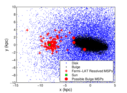
The Galactic Center Excess (GCE) is an extended gamma-ray source in the central region of the Galaxy found in Fermi Large Area Telescope (Fermi-LAT) data. One of the leading explanations for the GCE is an unresolved population of millisecond pulsars (MSPs) in the Galactic bulge. Due to differing star formation histories it is expected that the MSPs in the Galactic bulge are older and therefore dimmer than those in the Galactic disk. Additionally, correlations between the spectral parameters of the MSPs and the spin-down rate of the corresponding neutron stars have been observed. This implies that the bulge MSPs may be spectrally different from the disk MSPs. We perform detailed modelling of the MSPs from formation until observation. Although we confirm the correlations, we do not find they are sufficiently large to significantly differentiate the spectra of the bulge MSPs and disk MSPs when the uncertainties are accounted for. Our results demonstrate that the population of MSPs that can explain the gamma-ray signal from the resolved MSPs in the Galactic disk and the unresolved MSPs in the boxy bulge and nuclear bulge can consistently be described as arising from a common evolutionary trajectory for some subset of astrophysical sources common to all these different environments. We do not require that there is anything unusual about inner Galaxy MSPs to explain the GCE. Additionally, we use a more accurate geometry for the distribution of bulge MSPs and incorporate dispersion measure estimates of the MSPs’ distances. We find that the elongated boxy bulge morphology means that some the bulge MSPs are closer to us and so easier to resolve. We identify three resolved MSPs that have significant probabilities of belonging to the bulge population.

1 Introduction

Initially, the GCE appeared to be distributed spherically symmetrically around the Galactic Center with a radially-declining intensity. This, and the fact that it exhibits a spectral peak at a few GeV, suggested the possibility that it was evidence of weakly interacting massive particles (WIMPs) self-annihilating with a Navarro-Frenk-White (NFW) density profile [1, 2, 3, 4]. Evidence now suggests that, when examined in detail, the GCE is not in fact spherically symmetric but exhibits a spatial morphology correlated with stellar mass in the Galactic bulge [5, 6, 7, 8, 9]. This disfavors a dark matter origin for the GCE and rather points to a scenario in which it is produced by a population of dim, unresolved, astrophysical point sources such as MSPs [10]. There is some debate about whether the resolved MSPs are consistent with the needed bulge population, see for example refs. [11, 12, 13, 14].

In previous investigations, the spectrum of the MSPs in the bulge have been assumed to be the same as those in the disk. However, the bulge MSPs are expected to be on average older than the disk MSPs due to their different star formation histories [15]. Therefore, we would expected them to have on average lower luminosities. In addition to this, a correlation between luminosities on the spectral parameters is seen in the data [16, 17] and so one would expect the bulge MSPs to be spectrally different from the disk ones. This motivates the more detailed modelling of the MSP populations that is performed in the current article.

We extend the model of the Galactic population of gamma-ray millisecond pulsars (MSPs) of Ploeg et al. [13]. In the current article we use the dispersion measure estimates of the MSP distances and incorporate the corresponding uncertainties in the free electron densities. Also, instead of empirically parameterising the MSP luminosity function, we start from empirical distributions describing MSP initial period, magnetic field strength, age, and gamma-ray spectra. We assume there is a relationship between the luminosity of a pulsar and some of its other properties such as its period, period derivative or spectral energy cutoff. This supposition is motivated by work such as by Kalapotharakos et al. [17] in which, based on data on resolved MSPs and young pulsars in Abdo et al. [16], it was determined that there is a relationship between MSP luminosity, on the one hand, and MSP spectral energy cutoff Ecutsubscript𝐸cutE_{\rm cut}, magnetic field strength B𝐵B, and the spin-down power E˙˙𝐸\dot{E}, on the other. Specifically, Kalapotharakos et al. [17] found that gamma-ray emission from MSPs is via curvature radiation and scales like LEcut1.18±0.24B0.17±0.05E˙0.41±0.08proportional-to𝐿superscriptsubscript𝐸cutplus-or-minus1.180.24superscript𝐵plus-or-minus0.170.05superscript˙𝐸plus-or-minus0.410.08L\propto E_{\rm cut}^{1.18\pm 0.24}B^{0.17\pm 0.05}\dot{E}^{0.41\pm 0.08} where we use 68% confidence intervals when quoting uncertainties unless otherwise specified. Similarly, Gonthier et al. [18] assumed that the radio and gamma ray luminosities of MSPs were dependent on period and period derivative and, under this assumption, successfully determined the parameters of that relationship using a model of the distribution and properties of the Galactic population of MSPs, radio and gamma-ray detection thresholds, and a model of how the observed flux of an individual MSP depends on viewing angle and magnetic axis angle.

2 Method

To fit our model of the Galactic MSP population we used MSPs with confirmed gamma ray pulsations according to the Public List of LAT-Detected Gamma-Ray Pulsars111https://confluence.slac.stanford.edu/display/GLAMCOG/Public+List+of+LAT-Detected+Gamma-Ray+Pulsars. From that list, we obtained names and periods of pulsars. We then used the gamma-ray data for the corresponding sources in the Fermi Large Area Telescope fourth source catalog data release 2 [4FGL-DR2: 19]. Additional data was taken from the Australia Telescope National Facility (ATNF) pulsar catalog [20] if available. As in Bartels et al. [14] we used pulsars with periods less than 303030 ms that were not associated with globular clusters. For the Galactic Center Excess (GCE), we use the boxy bulge and nuclear bulge spectra222Available from https://github.com/chrisgordon1/Galactic_bulge_spectra. from Macias et al. [7]. We included both the systematic and statistical errors of these spectra which were added in quadrature to get the total error. The systematic error accounts for variation in the GCE spectra caused by using different maps of Inverse Compton emission.

2.1 Modeling the Galactic Millisecond Pulsar population

2.1.1 Spatial distribution

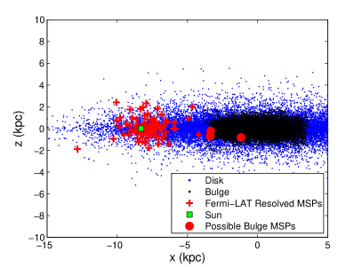
The spatial model of MSPs has three components: a disk distribution, a boxy bulge distribution, and a nuclear bulge distribution. The disk component models the population from which we expect the resolved MSPs to mainly come and has density:

ρdisk(R,z)exp(R2/2σr2)exp(|z|/z0)proportional-tosubscript𝜌disk𝑅𝑧superscript𝑅22superscriptsubscript𝜎𝑟2𝑧subscript𝑧0\rho_{\rm disk}(R,z)\propto\exp(-R^{2}/2\sigma_{r}^{2})\exp(-\absolutevalue{z}/z_{0}) (2.1)

where R2=x2+y2superscript𝑅2superscript𝑥2superscript𝑦2R^{2}=x^{2}+y^{2} is the radial coordinate in the Galactic disk and z𝑧z is the height above the Galactic Plane. We treat σrsubscript𝜎𝑟\sigma_{r} and z0subscript𝑧0z_{0} as free parameters to be fit to the data. The modeled GCE is produced by the boxy bulge and nuclear bulge components. The boxy bulge has density [21, 7]:

ρboxybulge(Rs)sech2(Rs)×{1RRendexp((RRend)2/hend2)R>Rendproportional-tosubscript𝜌boxybulgesubscript𝑅𝑠superscript2subscript𝑅𝑠cases1𝑅subscript𝑅endsuperscript𝑅subscript𝑅end2subscriptsuperscript2end𝑅subscript𝑅end\rho_{\rm boxy~{}bulge}(R_{s})\propto\sech^{2}(R_{s})\times\begin{cases}1&R\leq R_{\rm end}\\ \exp(-(R-R_{\rm end})^{2}/h^{2}_{\rm end})&R>R_{\rm end}\\ \end{cases} (2.2)

where Rend=3.128subscript𝑅end3.128R_{\rm end}=3.128 kpc, hend=0.461subscriptend0.461h_{\rm end}=0.461 kpc, and:

RC=(|x|1.696kpc)C+(|y|0.6426kpc)Csuperscriptsubscript𝑅perpendicular-tosubscript𝐶perpendicular-tosuperscriptsuperscript𝑥1.696kpcsubscript𝐶perpendicular-tosuperscriptsuperscript𝑦0.6426kpcsubscript𝐶perpendicular-toR_{\perp}^{C_{\perp}}=\left(\frac{\absolutevalue{x^{\prime}}}{1.696~{}\textrm{kpc}}\right)^{C_{\perp}}+\left(\frac{\absolutevalue{y^{\prime}}}{0.6426~{}\textrm{kpc}}\right)^{C_{\perp}} (2.3)
RsC=RC+(|z|0.4425kpc)Csuperscriptsubscript𝑅𝑠subscript𝐶parallel-tosuperscriptsubscript𝑅perpendicular-tosubscript𝐶parallel-tosuperscriptsuperscript𝑧0.4425kpcsubscript𝐶parallel-toR_{s}^{C_{\parallel}}=R_{\perp}^{C_{\parallel}}+\left(\frac{\absolutevalue{z^{\prime}}}{0.4425~{}\textrm{kpc}}\right)^{C_{\parallel}} (2.4)

where C=3.501subscript𝐶parallel-to3.501C_{\parallel}=3.501 and C=1.574subscript𝐶perpendicular-to1.574C_{\perp}=1.574. The coordinates xsuperscript𝑥x^{\prime}, ysuperscript𝑦y^{\prime} and zsuperscript𝑧z^{\prime} are Cartesian coordinates in the boxy bulge frame. Relative to the frame in which x=R0subscript𝑥direct-productsubscript𝑅0x_{\odot}=-R_{0}, y=z=0subscript𝑦direct-productsubscript𝑧direct-product0y_{\odot}=z_{\odot}=0, this frame is rotated 13.79superscript13.7913.79^{\circ} around the z-axis then 0.023superscript0.0230.023^{\circ} around the new y-axis. We assume R0=8.3subscript𝑅08.3R_{0}=8.3 kpc as adopted from the YMW16 free electron density model [22] which we use to convert between distance and dispersion measure The nuclear bulge MSP density is proportional to the sum of the mass densities of the nuclear stellar cluster (NSC) and nuclear stellar disk (NSD) [6]:

ρnuclearbulge(r,z)ρNSC(r)+ρNSD(r,z)proportional-tosubscript𝜌nuclearbulge𝑟𝑧subscript𝜌NSC𝑟subscript𝜌NSD𝑟𝑧\rho_{\rm nuclear~{}bulge}(r,z)\propto\rho_{\rm NSC}(r)+\rho_{\rm NSD}(r,z) (2.5)

where r2=x2+y2+z2superscript𝑟2superscript𝑥2superscript𝑦2superscript𝑧2r^{2}=x^{2}+y^{2}+z^{2} and where the NSC has density:

ρNSC(r)={ρ0,NSC1+(rr0)2r6pcρ1,NSC1+(rr0)36pc<r200pc0r>200pcsubscript𝜌NSC𝑟casessubscript𝜌0NSC1superscript𝑟subscript𝑟02𝑟6pcsubscript𝜌1NSC1superscript𝑟subscript𝑟036pc𝑟200pc0𝑟200pc\rho_{\rm NSC}(r)=\begin{cases}\frac{\rho_{0\rm,NSC}}{1+\left(\frac{r}{r_{0}}\right)^{2}}&r\leq 6~{}\textrm{pc}\\ \frac{\rho_{1\rm,NSC}}{1+\left(\frac{r}{r_{0}}\right)^{3}}&6~{}\textrm{pc}<r\leq 200~{}\textrm{pc}\\ 0&r>200~{}\textrm{pc}\end{cases} (2.6)

where r0=0.22pcsubscript𝑟00.22pcr_{0}=0.22~{}\textrm{pc}, ρ0,NSC=3.3×10⁶Mpc3subscript𝜌0NSC3.3superscript106subscriptMdirect-productsuperscriptpc3\rho_{0\rm,NSC}=3.3\times 10^{6}~{}\textrm{M}_{\odot}~{}\textrm{pc}^{-3} and ρ1,NSCsubscript𝜌1NSC\rho_{1\rm,NSC} is set so that ρNSC(r)subscript𝜌NSC𝑟\rho_{\rm NSC}(r) is continuous at r=6pc𝑟6pcr=6~{}\textrm{pc}. The NSD has density:

ρNSD(r,z)={ρ0,NSD(r1pc)0.1e|z|45pcr<120pcρ1,NSD(r1pc)3.5e|z|45pc120pcr<220pcρ2,NSD(r1pc)10e|z|45pcr220pcsubscript𝜌NSD𝑟𝑧casessubscript𝜌0NSDsuperscript𝑟1pc0.1superscript𝑒𝑧45pc𝑟120pcsubscript𝜌1NSDsuperscript𝑟1pc3.5superscript𝑒𝑧45pc120pc𝑟220pcsubscript𝜌2NSDsuperscript𝑟1pc10superscript𝑒𝑧45pc𝑟220pc\rho_{\rm NSD}(r,z)=\begin{cases}\rho_{0\rm,NSD}\left(\frac{r}{1~{}\textrm{pc}}\right)^{-0.1}e^{-\frac{\absolutevalue{z}}{45~{}\textrm{pc}}}&r<120~{}\textrm{pc}\\ \rho_{1\rm,NSD}\left(\frac{r}{1~{}\textrm{pc}}\right)^{-3.5}e^{-\frac{\absolutevalue{z}}{45~{}\textrm{pc}}}&120~{}\textrm{pc}\leq r<220~{}\textrm{pc}\\ \rho_{2\rm,NSD}\left(\frac{r}{1~{}\textrm{pc}}\right)^{-10}e^{-\frac{\absolutevalue{z}}{45~{}\textrm{pc}}}&r\geq 220~{}\textrm{pc}\end{cases} (2.7)

where ρ0,NSD=301Mpc3subscript𝜌0NSD301subscriptMdirect-productsuperscriptpc3\rho_{0\rm,NSD}=301~{}\textrm{M}_{\odot}~{}\textrm{pc}^{-3} and ρ1,NSDsubscript𝜌1NSD\rho_{1\rm,NSD} and ρ2,NSDsubscript𝜌2NSD\rho_{2\rm,NSD} are set so that ρNSD(r,z)subscript𝜌NSD𝑟𝑧\rho_{\rm NSD}(r,z) is continous at both r=120pc𝑟120pcr=120~{}\textrm{pc} and r=220pc𝑟220pcr=220~{}\textrm{pc}.

2.1.2 Age distribution

The MSP age distribution is dependent on two distributions: the star formation rate (SFR), and the delay time distribution (DTD). We assume for the DTD a five bin distribution between 0 Gyr and the age of the universe.

For the disk and boxy bulge components of the MSP population, the SFR is [15]:

SFR(z)=max(10Az2+Bz+CD,0)SFR𝑧superscript10𝐴superscript𝑧2𝐵𝑧𝐶𝐷0\textrm{SFR}(z)=\max(10^{Az^{2}+Bz+C}-D,0) (2.8)

where for the disk MSPs A=4.06×10²𝐴4.06superscript102A=-4.06\times 10^{-2}, B=0.331𝐵0.331B=0.331, C=0.338𝐶0.338C=0.338 and D=0.771𝐷0.771D=0.771. For the boxy bulge A=2.62×10²𝐴2.62superscript102A=-2.62\times 10^{-2}, B=0.384𝐵0.384B=0.384, C=8.42×10²𝐶8.42superscript102C=-8.42\times 10^{-2} and D=3.254𝐷3.254D=3.254. The relationship between cosmological time t𝑡t and redshift z𝑧z is [23]:

t(z)=9.778Gyrh01/(1+z)dxxΩΛ+ΩKx2+ΩMx3+ΩRx4𝑡𝑧9.778Gyrsubscriptsuperscript11𝑧0𝑥𝑥subscriptΩΛsubscriptΩ𝐾superscript𝑥2subscriptΩ𝑀superscript𝑥3subscriptΩ𝑅superscript𝑥4t(z)=\frac{9.778~{}\textrm{Gyr}}{h}\int^{1/(1+z)}_{0}\frac{\differential x}{x\sqrt{\Omega_{\Lambda}+\Omega_{K}x^{-2}+\Omega_{M}x^{-3}+\Omega_{R}x^{-4}}} (2.9)

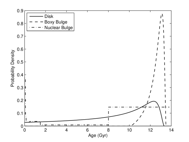
where we have used h=0.670.67h=0.67, ΩΛ=0.68subscriptΩΛ0.68\Omega_{\Lambda}=0.68, ΩM=1ΩΛsubscriptΩ𝑀1subscriptΩΛ\Omega_{M}=1-\Omega_{\Lambda} and ΩK=ΩR=0subscriptΩ𝐾subscriptΩ𝑅0\Omega_{K}=\Omega_{R}=0 [24]. For the nuclear bulge, we use the MIST star formation rate from Nogueras-Lara et al. [25]. The three star formation rates are shown in Fig. 1.
Refer to caption
Figure 1: Star formation rates for the disk, boxy bulge, and nuclear bulge. Here, this is given as a normalized probability density of stellar mass having formed at a particular age.

From the SFR and DTD, we can find the probability density function of MSP ages:

p(age)=0t0ageSFR(z(τ))DTD(t0ageτ)dτ0t00tSFR(z(τ))DTD(tτ)dτdt𝑝agesuperscriptsubscript0subscript𝑡0ageSFR𝑧𝜏DTDsubscript𝑡0age𝜏𝜏superscriptsubscript0subscript𝑡0superscriptsubscript0superscript𝑡SFR𝑧𝜏DTDsuperscript𝑡𝜏𝜏superscript𝑡p({\rm age})=\frac{\int_{0}^{t_{0}-{\rm age}}{\rm SFR}(z(\tau)){\rm DTD}(t_{0}-{\rm age}-\tau)\differential\tau}{\int_{0}^{t_{0}}\int_{0}^{t^{\prime}}{\rm SFR}(z(\tau)){\rm DTD}(t^{\prime}-\tau)\differential\tau\differential t^{\prime}} (2.10)

where t0subscript𝑡0t_{0} is the age of the universe, and z(t)𝑧𝑡z(t) is the inverse of Eq. 2.9.

As an alternative age distribution, we try a uniform distribution where MSPs form at a constant rate over the last 10 Gyr, similar to that assumed by Gonthier et al. [18].

2.1.3 Angular velocity

In our model, the angular transverse velocities of pulsars in the directions of Galactic longitude and latitude, μlsubscript𝜇𝑙\mu_{l} and μbsubscript𝜇𝑏\mu_{b} respectively, are determined by assuming a pulsar travels in a circular orbit around the center of the Galaxy using a parametric form of the potential [26, 27] with a random normally distributed peculiar velocity in every direction of scale σvsubscript𝜎𝑣\sigma_{v} (i.e., a Maxwell distribution). For the Sun, we assume circular motion in the same potential with a peculiar velocity of (11.1, 12.24, 7.25) km s-1 where the velocity components are in the direction of the Galactic Center, the direction of rotation and in the direction perpendicular to the plane, respectively [28]. The relationship between velocity (v𝑣v) and angular velocity (μ𝜇\mu) at a distance d𝑑d is:

v4.74(dkpc)(μ mas yr1) km s1𝑣4.74𝑑kpc𝜇superscript mas yr1superscript km s1v\approx 4.74\left(\frac{d}{\textrm{kpc}}\right)\left(\frac{\mu}{\textrm{ mas yr}^{-1}}\right)\textrm{ km s}^{-1} (2.11)

2.1.4 Galactic Center Excess

To simulate the GCE, we need to assign each bulge MSP a spectrum that describes its photon number flux (N𝑁N) at energy E𝐸E:

dNdE=KEΓexp((E/Ecut)2/3)𝑁𝐸𝐾superscript𝐸Γsuperscript𝐸subscript𝐸cut23\frac{\differential N}{\differential E}=KE^{-\Gamma}\exp(-\left(E/E_{\rm cut}\right)^{2/3}) (2.12)

where the spectral parameters are K𝐾K, ΓΓ\Gamma, and Ecutsubscript𝐸cutE_{\rm cut}. The proportionality constant K𝐾K is determined via:

F=0.1 GeV100 GeVEdNdEdE𝐹superscriptsubscript0.1 GeV100 GeV𝐸𝑁𝐸𝐸F=\int_{0.1\textrm{ GeV}}^{100\textrm{ GeV}}E\frac{\differential N}{\differential E}\differential E (2.13)

where F𝐹F is the energy flux. The simulated boxy bulge and nuclear bulge GCE spectra are then the sum of all MSP spectra in each of those two bulge populations of MSPs. This spectrum is equivalent to the one used to fit the resolved MSPs in the 4FGL-DR2 catalog [19] and it will also be the one we use for our resolved MSPs.

2.1.5 Millisecond pulsar parameters

Force-free electrodynamic solutions have given the following expression for the spin-down luminosity [29]

Lsdμ2Ω4c3(1+sin2α)similar-tosubscript𝐿sdsuperscript𝜇2superscriptΩ4superscript𝑐31superscript2𝛼L_{\mathrm{sd}}\sim\frac{\mu^{2}\Omega^{4}}{c^{3}}\left(1+\sin^{2}\alpha\right) (2.14)

where μ𝜇\mu is the magnetic dipole moment, ΩΩ\Omega is the rotational angular velocity, c𝑐c is the speed of light, and α𝛼\alpha is the angle between the rotation and magnetic field axes. The magnetic field strength (B𝐵B) at the magnetic pole of the star is related to μ𝜇\mu by [29]

μ=BR32𝜇𝐵superscript𝑅32\mu=\frac{BR^{3}}{2} (2.15)

where R𝑅R is the radius of the neutron star and we use R=12km𝑅12kmR=12~{}\textrm{km}. The rotational kinetic energy of the neutron star is given by the standard formula for a rotating body

E=12IΩ2𝐸12𝐼superscriptΩ2E=\frac{1}{2}I\Omega^{2} (2.16)

where I𝐼I is the neutron star’s moment of inertia and we use I=1.7×1045g cm2𝐼1.7superscript1045superscriptg cm2I=1.7\times 10^{45}~{}\textrm{g cm}^{2}. Therefore, the spin-down power satisfies

E˙=4π2IP˙int/P3˙𝐸4superscript𝜋2𝐼subscript˙𝑃intsuperscript𝑃3\dot{E}=4\pi^{2}I\dot{P}_{\rm int}/P^{3} (2.17)

where P˙intsubscript˙𝑃int\dot{P}_{\rm int} is the time derivative of the intrinsic period, which may be different to the observed period derivative (P˙˙𝑃\dot{P}), and P=2π/Ω𝑃2𝜋ΩP=2\pi/\Omega is the period. Equating the spin-down luminosity (Eq. 2.14) to the spin down power (Eq. 2.17) and using Eq. 2.15 yields the following expression for the magnetic field strength of an MSP

B2=c3IPP˙intπ2R6(1+sin2(α)).superscript𝐵2superscript𝑐3𝐼𝑃subscript˙𝑃intsuperscript𝜋2superscript𝑅61superscript2𝛼B^{2}=\frac{c^{3}IP\dot{P}_{\rm int}}{\pi^{2}R^{6}(1+\sin^{2}(\alpha))}. (2.18)

The angle α𝛼\alpha is chosen randomly from the probability density:

p(α)=12sin(α)𝑝𝛼12𝛼p(\alpha)=\frac{1}{2}\sin(\alpha) (2.19)

which corresponds to a uniformly random magnetic field axis relative to the rotation axis.

The intrinsic period time derivative is related to the observed period time derivative P˙˙𝑃\dot{P} by [16]:

P˙=P˙int+P˙Shklovskii+P˙Galactic˙𝑃subscript˙𝑃intsubscript˙𝑃Shklovskiisubscript˙𝑃Galactic\dot{P}=\dot{P}_{\rm int}+\dot{P}_{\rm Shklovskii}+\dot{P}_{\rm Galactic} (2.20)

where the contribution to the observed period derivative from the Shklovskii effect is given by

P˙Shklovskii=2.43×10²¹(μmas yr1)2(dkpc)(Ps)subscript˙𝑃Shklovskii2.43superscript1021superscript𝜇superscriptmas yr12𝑑kpc𝑃s\dot{P}_{\rm Shklovskii}=2.43\times 10^{-21}\left(\frac{\mu}{\textrm{mas yr}^{-1}}\right)^{2}\left(\frac{d}{\textrm{kpc}}\right)\left(\frac{P}{\textrm{s}}\right) (2.21)

and the contribution due to the relative acceleration in the Galactic potential is:

P˙Galactic=1c𝒏10(𝒂p𝒂)Psubscript˙𝑃Galactic1𝑐subscript𝒏10subscript𝒂𝑝subscript𝒂direct-product𝑃\dot{P}_{\rm Galactic}=\frac{1}{c}\bm{n}_{10}\cdot(\bm{a}_{p}-\bm{a}_{\odot})P (2.22)

where 𝒏10subscript𝒏10\bm{n}_{10} is the unit vector from the Sun to the pulsar, and 𝒂psubscript𝒂𝑝\bm{a}_{p} and 𝒂subscript𝒂direct-product\bm{a}_{\odot} are the accelerations, due to the Galactic potential [26, 27], of the pulsar and Sun respectively. Note that P=(1+vR/c)Pint𝑃1subscript𝑣R𝑐subscript𝑃intP=\left(1+v_{\mathrm{R}}/c\right)P_{\mathrm{int}}, where vRsubscript𝑣Rv_{\mathrm{R}} is the radial velocity of the pulsar and Pintsubscript𝑃intP_{\mathrm{int}} is the intrinsic period. Given vRcmuch-less-thansubscript𝑣R𝑐v_{\mathrm{R}}\ll c, we approximate Pint=Psubscript𝑃int𝑃P_{\mathrm{int}}=P. Making the common assumption that magnetic field strength remains constant over time, Eq. 2.18 results in:

P=PI2+2π2R6Ic3(1+sin2(α))B2t𝑃superscriptsubscript𝑃𝐼22superscript𝜋2superscript𝑅6𝐼superscript𝑐31superscript2𝛼superscript𝐵2𝑡P=\sqrt{P_{I}^{2}+\frac{2\pi^{2}R^{6}}{Ic^{3}}(1+\sin^{2}(\alpha))B^{2}t} (2.23)

where PIsubscript𝑃𝐼P_{I} is the initial period of the MSP at birth and t𝑡t is the age.

We consider multiple relationships between pulsar parameters and the 0.10.10.1-100100100 GeV luminosity (L𝐿L). Our most general form is that used by Kalapotharakos et al. [17]:

L=ηEcutaγBbγE˙dγ𝐿𝜂superscriptsubscript𝐸cutsubscript𝑎𝛾superscript𝐵subscript𝑏𝛾superscript˙𝐸subscript𝑑𝛾L=\eta E_{\rm cut}^{a_{\gamma}}B^{b_{\gamma}}\dot{E}^{d_{\gamma}} (2.24)

where η𝜂\eta is a proportionality factor. We also consider the model used by Gonthier et al. [18]:

L=ηPαγP˙βγ.𝐿𝜂superscript𝑃subscript𝛼𝛾superscript˙𝑃subscript𝛽𝛾L=\eta P^{\alpha_{\gamma}}\dot{P}^{\beta_{\gamma}}\,. (2.25)

The simplest form we consider is that the luminosity is an entirely independent parameter as used by Ploeg et al. [13]:

L=η.𝐿𝜂L=\eta\,. (2.26)

The likelihood probability density distributions of B𝐵B, Ecutsubscript𝐸cutE_{\rm cut}, and η𝜂\eta are assumed to be log-normal as this functional form gives a good fit to their histogrammed data of the resolved Fermi-LAT MSPs:

p(log10(x)|xmed,σx)=12πσxexp((log10(x)log10(xmed))22σx2)𝑝conditionalsubscript10𝑥subscript𝑥medsubscript𝜎𝑥12𝜋subscript𝜎𝑥superscriptsubscript10𝑥subscript10subscript𝑥med22superscriptsubscript𝜎𝑥2p(\log_{10}(x)|x_{\rm med},\sigma_{x})=\frac{1}{\sqrt{2\pi}\sigma_{x}}\exp\left(-\frac{\left(\log_{10}(x)-\log_{10}(x_{\rm med})\right)^{2}}{2\sigma_{x}^{2}}\right) (2.27)

where xmedsubscript𝑥medx_{\rm med} is the median of x𝑥x and σxsubscript𝜎𝑥\sigma_{x} is the standard deviation of log10(x)subscript10𝑥\log_{10}(x). We also assume PIsubscript𝑃𝐼P_{I} has this form but our results are not sensitive to to this assumption. In particular, we found that the cut off power law model used by Gonthier et al. [18] gives similar results. Note that, even though Ecutsubscript𝐸cutE_{\rm cut} is obtained from a fit of an individual MSP’s spectral data, for our purposes it is treated as a directly measured datum rather than a parameter to be estimated.

Fits to the MSP gamma-ray data [16] have uncovered correlations between the spectral parameters and E˙˙𝐸\dot{E}. To allow for this to potentially be an intrinsic property of the MSPs, we parameterise the median of the Ecutsubscript𝐸cutE_{\rm cut} likelihood as:

log10(Ecut,med/MeV)=aEcutlog10(E˙/(1034.5 erg s1))+bEcutsubscript10subscript𝐸cutmedMeVsubscript𝑎subscript𝐸cutsubscript10˙𝐸superscript1034.5superscript erg s1subscript𝑏subscript𝐸cut\log_{10}(E_{\rm cut,med}/\text{MeV})=a_{E_{\rm cut}}\log_{10}(\dot{E}/(10^{34.5}\textrm{ erg s}^{-1}))+b_{E_{\rm cut}} (2.28)

where aEcutsubscript𝑎subscript𝐸cuta_{E_{\rm cut}} and bEcutsubscript𝑏subscript𝐸cutb_{E_{\rm cut}} are allowed to vary in our model fits. We also model the likelihood of spectral index ΓΓ\Gamma using a normal distribution with mean μΓsubscript𝜇Γ\mu_{\Gamma} and standard deviation σΓsubscript𝜎Γ\sigma_{\Gamma}. We assume that

μΓ=aΓlog10(E˙/(1034.5 erg s1))+bΓsubscript𝜇Γsubscript𝑎Γsubscript10˙𝐸superscript1034.5superscript erg s1subscript𝑏Γ\mu_{\Gamma}=a_{\Gamma}\log_{10}(\dot{E}/(10^{34.5}\textrm{ erg s}^{-1}))+b_{\Gamma} (2.29)

where aΓsubscript𝑎Γa_{\Gamma} and bΓsubscript𝑏Γb_{\Gamma} are parameters. We also have a correlation coefficient, rΓ,Ecutsubscript𝑟Γsubscript𝐸cutr_{\Gamma,E_{\rm cut}} between ΓΓ\Gamma and log10(Ecut)subscript10subscript𝐸cut\log_{10}(E_{\rm cut}), so the likelihood is:

p(Γ,log10(Ecut)|𝜽)=12πσΓσEcut1rΓ,Ecut2exp(zΓ,Ecut2(1rΓ,Ecut2))𝑝Γconditionalsubscript10subscript𝐸cut𝜽12𝜋subscript𝜎Γsubscript𝜎subscript𝐸cut1superscriptsubscript𝑟Γsubscript𝐸cut2subscript𝑧Γsubscript𝐸cut21superscriptsubscript𝑟Γsubscript𝐸cut2p(\Gamma,\log_{10}(E_{\rm cut})|\boldsymbol{\theta})=\frac{1}{2\pi\sigma_{\Gamma}\sigma_{E_{\rm cut}}\sqrt{1-r_{\Gamma,E_{\rm cut}}^{2}}}\exp\left(-\frac{z_{\Gamma,E_{\rm cut}}}{2(1-r_{\Gamma,E_{\rm cut}}^{2})}\right) (2.30)

where:

zΓ,Ecut=(ΓμΓ)2σΓ2+(log10(Ecut)log10(Ecut,med))2σEcut22rΓ,Ecut(ΓμΓ)(log10(Ecut)log10(Ecut,med))σΓσEcut.subscript𝑧Γsubscript𝐸cutsuperscriptΓsubscript𝜇Γ2superscriptsubscript𝜎Γ2superscriptsubscript10subscript𝐸cutsubscript10subscript𝐸cutmed2superscriptsubscript𝜎subscript𝐸cut22subscript𝑟Γsubscript𝐸cutΓsubscript𝜇Γsubscript10subscript𝐸cutsubscript10subscript𝐸cutmedsubscript𝜎Γsubscript𝜎subscript𝐸cutz_{\Gamma,E_{\rm cut}}=\frac{\left(\Gamma-\mu_{\Gamma}\right)^{2}}{\sigma_{\Gamma}^{2}}+\frac{\left(\log_{10}(E_{\rm cut})-\log_{10}(E_{\rm cut,med})\right)^{2}}{\sigma_{E_{\rm cut}}^{2}}-\frac{2r_{\Gamma,E_{\rm cut}}\left(\Gamma-\mu_{\Gamma}\right)\left(\log_{10}(E_{\rm cut})-\log_{10}(E_{\rm cut,med})\right)}{\sigma_{\Gamma}\sigma_{E_{\rm cut}}}\,. (2.31)

Note that here and in the rest of this article we will use 𝜽𝜽\boldsymbol{\theta} to indicate the relevant model parameters. In this case they are 𝜽={aEcut,bEcut,aΓ,BΓ,σEcut,σΓ,rΓ,Ecut}𝜽subscript𝑎subscript𝐸cutsubscript𝑏subscript𝐸cutsubscript𝑎Γsubscript𝐵Γsubscript𝜎subscript𝐸cutsubscript𝜎Γsubscript𝑟Γsubscript𝐸cut\boldsymbol{\theta}=\{a_{E_{\rm cut}},b_{E_{\rm cut}},a_{\Gamma},B_{\Gamma},\sigma_{E_{\rm cut}},\sigma_{\Gamma},r_{\Gamma,E_{\rm cut}}\}. See Table 1 for the corresponding priors that we use.

As alternatives, we try two likelihoods of PIsubscript𝑃𝐼P_{I} where there is a dependence on B𝐵B. In the first, a bivariate normal distribution relating log10(B)subscript10𝐵\log_{10}(B) and log10(PI)subscript10subscript𝑃𝐼\log_{10}(P_{I}) with a correlation parameter rB,PIsubscript𝑟𝐵subscript𝑃𝐼r_{B,P_{I}} is assumed. In the second, we adopt the relationship used by Gonthier et al. [18]:

PI=0.18×10CPI+3δ/7B86/7mssubscript𝑃𝐼0.18superscript10subscript𝐶subscript𝑃𝐼3𝛿7superscriptsubscript𝐵867msP_{I}=0.18\times 10^{C_{P_{I}}+3\delta/7}B_{8}^{6/7}\textrm{ms} (2.32)

where there is a lower bound of 1.31.31.3 ms, δ𝛿\delta is drawn from a uniform distribution between 00 and 222. Also, B8=(B/108G)subscript𝐵8𝐵superscript108GB_{8}=(B/10^{8}\textrm{G}). We fit CPIsubscript𝐶subscript𝑃𝐼C_{P_{I}} as model parameter while it is set to 00 by Gonthier et al. [18].

2.1.6 Millisecond pulsar detection

The flux of an MSP is related to the luminosity in the usual way:

F=L4πd2𝐹𝐿4𝜋superscript𝑑2F=\frac{L}{4\pi d^{2}} (2.33)

and the MSP detection threshold flux Fthsubscript𝐹thF_{\rm th} is drawn from a log-normal distribution so that the probability of a detection is [11, 13, 14]:

p(FthF|l,b,𝜽)=12(1+erf(log10(F)(log10(μth(l,b))+Kth)2σth))𝑝subscript𝐹thconditional𝐹𝑙𝑏𝜽121error-functionsubscript10𝐹subscript10subscript𝜇th𝑙𝑏subscript𝐾th2subscript𝜎thp(F_{\rm th}\leq F|l,b,\boldsymbol{\theta})=\frac{1}{2}\left(1+\erf\left(\frac{\log_{10}(F)-\left(\log_{10}(\mu_{\rm th}(l,b))+K_{\rm th}\right)}{\sqrt{2}\sigma_{\rm th}}\right)\right) (2.34)

where a map in longitude (l𝑙l) and latitude (b𝑏b) of μth(l,b)subscript𝜇th𝑙𝑏\mu_{\rm th}(l,b) associated with the 4FGL-DR2 catalog can be found online333https://fermi.gsfc.nasa.gov/ssc/data/access/lat/10yr_catalog/.

2.2 Fitting the model to data

To fit the model parameters to the resolved MSP and GCE data, we use an adaptive Markov Chain Monte Carlo (MCMC) algorithm [30]. The resolved MSPs have an unbinned Poisson likelihood [31]:

resexp(λres)i=1Nresρ(𝑫i)proportional-tosubscriptressubscript𝜆ressuperscriptsubscriptproduct𝑖1subscript𝑁res𝜌subscript𝑫𝑖\mathcal{L}_{\rm res}\propto\exp(-\lambda_{\rm res})\prod_{i=1}^{N_{\rm res}}\rho(\boldsymbol{D}_{i}) (2.35)

where Nressubscript𝑁resN_{\rm res} is the number of resolved MSPs, λressubscript𝜆res\lambda_{\rm res} is the expected number of resolved MSPs, and ρ(𝑫i)𝜌subscript𝑫𝑖\rho(\boldsymbol{D}_{i}) is the phase space density of the resolved MSPs which have the data

𝑫i={li,bi,di,Pi,P˙i,μl,i,μb,i,Fi,Ecut,i,Γi}.subscript𝑫𝑖subscript𝑙𝑖subscript𝑏𝑖subscript𝑑𝑖subscript𝑃𝑖subscript˙𝑃𝑖subscript𝜇𝑙𝑖subscript𝜇𝑏𝑖subscript𝐹𝑖subscript𝐸cut𝑖subscriptΓ𝑖\boldsymbol{D}_{i}=\{l_{i},b_{i},d_{i},P_{i},\dot{P}_{i},\mu_{l,i},\mu_{b,i},F_{i},E_{{\rm cut},i},\Gamma_{i}\}\,. (2.36)

That is, the resolved MSP is located at longitude lisubscript𝑙𝑖l_{i}, latitude bisubscript𝑏𝑖b_{i}, distance disubscript𝑑𝑖d_{i}, period Pisubscript𝑃𝑖P_{i}, observed period derivative P˙isubscript˙𝑃𝑖\dot{P}_{i}, proper motion in longitude μl,isubscript𝜇𝑙𝑖\mu_{l,i}, proper motion in latitude μb,isubscript𝜇𝑏𝑖\mu_{b,i}, flux Fisubscript𝐹𝑖F_{i}, spectrum energy cut-off Ecut,isubscript𝐸cut𝑖E_{{\rm cut},i}, and spectral index ΓisubscriptΓ𝑖\Gamma_{i}.

The expected number of resolved MSPs can be obtained by integrating the phase space density over the phase space volume as follows [31]:

λres=ρ(𝑫i)d𝑫isubscript𝜆res𝜌subscript𝑫𝑖differential-dsubscript𝑫𝑖\lambda_{\rm res}=\int\rho(\boldsymbol{D}_{i})\,{\rm d}{\boldsymbol{D}_{i}} (2.37)

This relation implies that

ρ(𝑫i)=p(𝑫i|obs,𝜽)λres𝜌subscript𝑫𝑖𝑝conditionalsubscript𝑫𝑖obs𝜽subscript𝜆res\rho(\boldsymbol{D}_{i})=p(\boldsymbol{D}_{i}|{\rm obs},\boldsymbol{\theta})\lambda_{\rm res} (2.38)

where obsobs{\rm obs} indicates the MSP was observed, i.e. it was resolved. Also, p(𝑫i|obs,θ)𝑝conditionalsubscript𝑫𝑖obs𝜃p(\boldsymbol{D}_{i}|{\rm obs},\theta) is the probability density that a resolved MSP has data 𝑫isubscript𝑫𝑖\boldsymbol{D}_{i} given that the model parameter values are θ𝜃\theta. It then follows from the above two equations that

p(𝑫i|obs,𝜽)d𝑫i=1𝑝conditionalsubscript𝑫𝑖obs𝜽differential-dsubscript𝑫𝑖1\int p(\boldsymbol{D}_{i}|{\rm obs},\boldsymbol{\theta})\,{\rm d}{\boldsymbol{D}_{i}}=1 (2.39)

as required.

There are many tens of thousands of unresolved MSPs in the Milky Way [13, 18] and we have only resolved of order 100 in gamma rays. It follows that the probability of observing an individual MSP must be a very small. Therefore, from the law of rare events (see for example Section 1.1.1 of [32]), the total number of resolved and unresolved MSPs (Ntotsubscript𝑁totN_{\rm tot}) is well approximated by:

Ntot=λres/p(obs|𝜽).subscript𝑁totsubscript𝜆res𝑝conditionalobs𝜽N_{\rm tot}=\lambda_{\rm res}/p(\rm obs|\boldsymbol{\theta})\,. (2.40)

We can find p(obs|𝜽)𝑝conditionalobs𝜽p({\rm obs}|\boldsymbol{\theta}) by noting that a luminosity threshold distribution p(Lth)𝑝subscript𝐿thp(L_{\rm th}) is determined by the combination of the flux threshold and spatial distributions. Thus:

p(obs|𝜽)=dLthp(Lth)p(LLth)𝑝conditionalobs𝜽subscript𝐿th𝑝subscript𝐿th𝑝𝐿subscript𝐿thp({\rm obs}|\boldsymbol{\theta})=\int\differential L_{\rm th}p(L_{\rm th})p(L\geq L_{\rm th}) (2.41)

where p(LLth)𝑝𝐿subscript𝐿thp(L\geq L_{\rm th}) is the probability that the luminosity is greater than or equal to the threshold. Another useful relation that follows from standard probability theory is:

p(obs,𝑫i|𝜽)=p(𝑫i|obs,𝜽)p(obs|𝜽).𝑝obsconditionalsubscript𝑫𝑖𝜽𝑝conditionalsubscript𝑫𝑖obs𝜽𝑝conditionalobs𝜽p({\rm obs},\boldsymbol{D}_{i}|\boldsymbol{\theta})=p(\boldsymbol{D}_{i}|{\rm obs},\boldsymbol{\theta})p({\rm obs}|\boldsymbol{\theta})\,. (2.42)

Combining the above equation with Eqs. 2.40 and 2.38 gives

ρ(𝑫i)=p(obs,𝑫i|𝜽)Ntot.𝜌subscript𝑫𝑖𝑝obsconditionalsubscript𝑫𝑖𝜽subscript𝑁tot\rho(\boldsymbol{D}_{i})=p({\rm obs},\boldsymbol{D}_{i}|\boldsymbol{\theta})N_{\rm tot}\,. (2.43)

We have two distinct types of resolved MSPs: those with parallax measurements and those without. To accommodate this we have two separate probability density functions

p(obs,𝑫i|𝜽)=p(obs,𝑫i,parallaxi|𝜽)+p(obs,𝑫i,not parallaxi|𝜽)𝑝obsconditionalsubscript𝑫𝑖𝜽𝑝obssubscript𝑫𝑖conditionalsubscriptparallax𝑖𝜽𝑝obssubscript𝑫𝑖conditionalsubscriptnot parallax𝑖𝜽p({\rm obs},\boldsymbol{D}_{i}|\boldsymbol{\theta})=p({\rm obs},\boldsymbol{D}_{i},{\rm parallax}_{i}|\boldsymbol{\theta})+p({\rm obs},\boldsymbol{D}_{i},\textrm{not parallax}_{i}|\boldsymbol{\theta}) (2.44)

The 𝑫isubscript𝑫𝑖\boldsymbol{D}_{i} components are the same in both cases as we can estimate the distance for those MSPs that do not have parallax measurements by their dispersion measures. The probability of a parallax measurement given distance d𝑑d is modelled as:

p(parallaxi|di,𝜽)=min(1,Cparallaxexp(di/dparallax)).𝑝conditionalsubscriptparallax𝑖subscript𝑑𝑖𝜽1subscript𝐶parallaxsubscript𝑑𝑖subscript𝑑parallaxp(\textrm{parallax}_{i}|d_{i},\boldsymbol{\theta})=\min(1,C_{\rm parallax}\exp(-d_{i}/d_{\rm parallax}))\,. (2.45)

and p(not parallaxi|di,𝜽)=1p(parallaxi|di,𝜽)𝑝conditionalsubscriptnot parallax𝑖subscript𝑑𝑖𝜽1𝑝conditionalsubscriptparallax𝑖subscript𝑑𝑖𝜽p(\textrm{not parallax}_{i}|d_{i},\boldsymbol{\theta})=1-p(\textrm{parallax}_{i}|d_{i},\boldsymbol{\theta}). See Appendix A for more details.

To take into account measurement uncertainty in our values of 𝑫isubscript𝑫𝑖\boldsymbol{D}_{i} we marginalise over the true values 𝑫^isubscript^𝑫𝑖\hat{\boldsymbol{D}}_{i}

p(obs,𝐃i|θ)=p(𝐃i|𝐃^i)p(obs,𝐃^i|𝜽)d𝐃^i𝑝obsconditionalsubscript𝐃i𝜃pconditionalsubscript𝐃isubscript^𝐃ipobsconditionalsubscript^𝐃i𝜽differential-dsubscript^𝐃ip(\rm obs,\boldsymbol{D}_{i}|\theta)=\int p(\boldsymbol{D}_{i}|\hat{\boldsymbol{D}}_{i})p({\rm obs},\hat{\boldsymbol{D}}_{i}|\boldsymbol{\theta})\,{\rm d}\hat{\boldsymbol{D}}_{i} (2.46)

If MSP i𝑖i has the j𝑗jth component of its data 𝑫isubscript𝑫𝑖\boldsymbol{D}_{i} missing then we account for that by making p(𝑫i|𝑫^i)𝑝conditionalsubscript𝑫𝑖subscript^𝑫𝑖p(\boldsymbol{D}_{i}|\hat{\boldsymbol{D}}_{i}) uniform in the j𝑗jth component. See Appendix B for more details.

We fit the boxy bulge and nuclear bulge GCE to spectra found by Macias et al. [7]. We use a Gaussian likelihood for each bin in the GCE spectra:

GCEi=1Nexp(((dNdE)sim,i(dNdE)data,i)2/(2σdata,i2))proportional-tosubscriptGCEsuperscriptsubscriptproduct𝑖1𝑁superscriptsubscript𝑁𝐸sim,𝑖subscript𝑁𝐸data,𝑖22subscriptsuperscript𝜎2data,𝑖\mathcal{L}_{\rm GCE}\propto\prod_{i=1}^{N}\exp(-\left(\left(\frac{\differential N}{\differential E}\right)_{\textrm{sim,}i}-\left(\frac{\differential N}{\differential E}\right)_{\textrm{data,}i}\right)^{2}/\left(2\sigma^{2}_{\textrm{data,}i}\right)) (2.47)

where (dNdE)sim,isubscript𝑁𝐸sim,𝑖\left(\frac{\differential N}{\differential E}\right)_{\textrm{sim,}i} is the simulated GCE for bin i𝑖i and (dNdE)data,isubscript𝑁𝐸data,𝑖\left(\frac{\differential N}{\differential E}\right)_{\textrm{data,}i} is the data with uncertainty σdata,i2subscriptsuperscript𝜎2data,𝑖\sigma^{2}_{\textrm{data,}i}. We fit only energy bins lower than 101010 GeV as the higher energy bins may contain significant secondary emission [7]. The combined likelihood for our resolved MSPs and the GCE is then given by substituting Eqs. 2.47 and 2.35 into

total=res×GCE.subscripttotalsubscriptressubscriptGCE\mathcal{L}_{\rm total}=\mathcal{L}_{\rm res}\times\mathcal{L}_{\rm GCE}\,. (2.48)

This is then multiplied with the priors given in Table 1 to get the posterior which is then sampled using MCMC. To test our models we generate posterior predictive distributions [33]. See Appendix C for more details on the sampling methods we used.

3 Results

In this section we present results for various assumed luminosity functions, age distributions, and relationships between magnetic field strength and initial period. We rank these various models using the Watanabe Akaike Information Criterion (WAIC) [34, 33] as described in Appendix D and given in Eq. D.12. The WAIC provides a measure of the expected predictive accuracy of a model and it takes into account the number of model parameters and their posterior uncertainty. Under suitable regularity conditions, in the limit of a large amount of data, the difference in the WAIC between two models (ΔΔ\DeltaWAIC) tends towards minus two times the log of their likelihood ratio [33]. So when adding an extra parameter to a model, the “number of sigma” in favour of adding that parameter is given approximately by ΔWAICΔWAIC\sqrt{\Delta{\rm WAIC}} [35]. This provides a rough benchmark in evaluating the significance of ΔΔ\DeltaWAIC values.

We can gain a more detailed view of a model’s fit by comparing its posterior predictive distributions to data using single dimensional binned plots showing medians and 68%percent6868\% and 95%percent9595\% intervals, as well as corner plots constructed using the software by Foreman-Mackey [36]. These posterior predictive distributions provide an effective method of evaluating the goodness of fit [33, 37]. In particular, major failures of the model correspond to extreme posterior predictive p-values. These are defined as the proportion of posterior simulations which are more extreme than the data or some statistic of the data [33]. Our corner plots show two dimensional distributions of real data and simulated data with 68%percent6868\%, 95%percent9595\% and 99.7%percent99.799.7\% contours. In producing simulated data we model both missing data and uncertainties by picking a random real MSP and removing simulated data that is not available for the real MSP. For data with uncertainties attached, we take the relative error for the real MSP and add Gaussian noise to the simulated MSP which has a standard deviation with the same relative error as the real MSP. We have a distance dependent model of the probability of a parallax measurement being available. If a simulated MSP has a parallax measurement, with probability given by Eq. 2.45, we select a random real MSP out of those with available parallax measurements and use its relative uncertainty to simulate a parallax error.

The WAIC allows us to compare the various models used while accounting for the varying number of parameters they involve. In Table 2 we show the WAIC averaged over the eight chains for each of a set of models of the Galactic MSP population relative to that of the best model. We also show the sample standard deviation over the WAIC for the eight MCMC chains run for each model. This variation occurs because we used Monte Carlo integration to compute the integrals in Section 2. The random numbers used to compute these integrals (such as over the resolved MSP data uncertainty distributions) were generated once per MCMC chain so that a calculation of the likelihood for a given set of parameters will always return the same result. However, between chains the likelihood may shift slightly as the set of randomly generated numbers used will be different. As a result of this variation in the likelihood, we did not generate a single WAIC for all eight chains combined. We found that the posterior distributions of the model parameters were generally indistinguishable despite these variations, and the variation in WAIC for each model is typically small compared to ΔWAICΔWAIC\Delta\textrm{WAIC} between models.

In Table 3 we report medians and 68%percent6868\% confidence intervals for the parameters of a subset of these models. The first three parameters in this table are related to the number of MSPs in each of the three spatial components of the model: The parameter λressubscript𝜆res\lambda_{\rm res} is the expected number of resolved MSPs; log10(Ndisk/Nbulge)subscript10subscript𝑁disksubscript𝑁bulge\log_{10}(N_{\rm disk}/N_{\rm bulge}) and log10(Nnb/Nbb)subscript10subscript𝑁nbsubscript𝑁bb\log_{10}(N_{\rm nb}/N_{\rm bb}) are parameters defining, respectively, the ratio of Ndisksubscript𝑁diskN_{\rm disk} to Nbulgesubscript𝑁bulgeN_{\rm bulge} and Nnbsubscript𝑁nbN_{\rm nb} to Nbbsubscript𝑁bbN_{\rm bb}. Here Ndisksubscript𝑁diskN_{\rm disk} is the number of disk MSPs, Nbulge=Nnb+Nbbsubscript𝑁bulgesubscript𝑁nbsubscript𝑁bbN_{\rm bulge}=N_{\rm nb}+N_{\rm bb} is the total number of bulge MSPs, Nnbsubscript𝑁nbN_{\rm nb} is the number of nuclear bulge MSPs, and Nbbsubscript𝑁bbN_{\rm bb} is the number of boxy bulge MSPs.

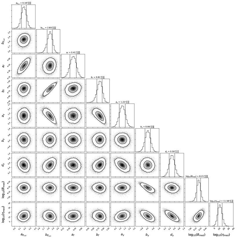
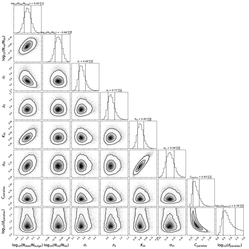
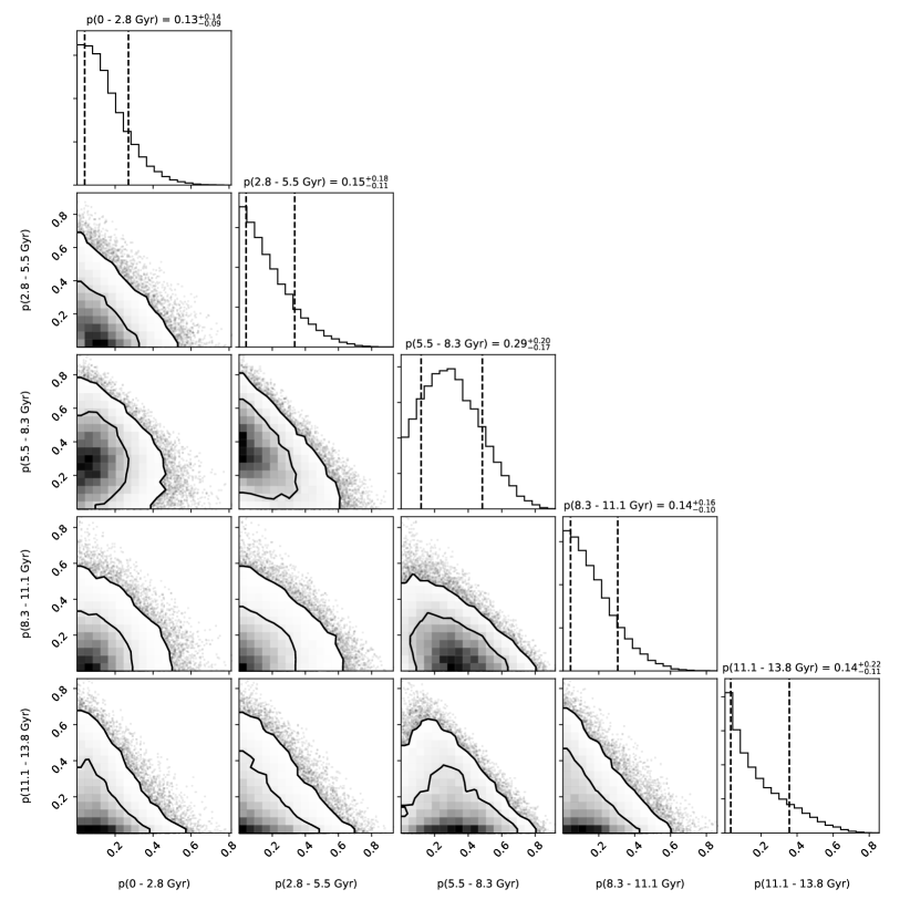
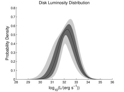
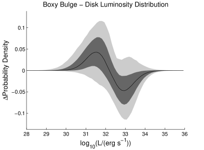
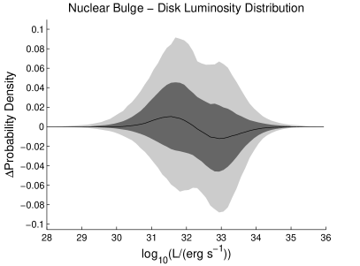
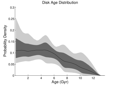
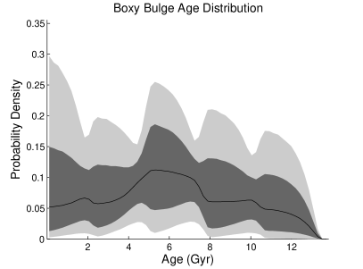
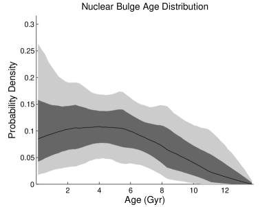
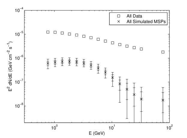
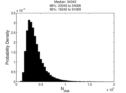
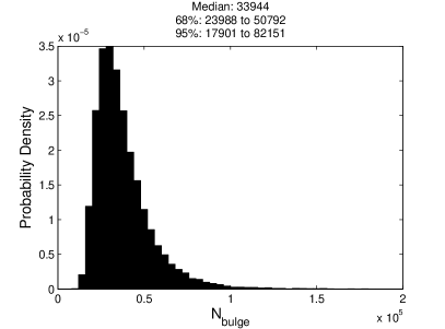
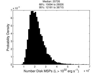
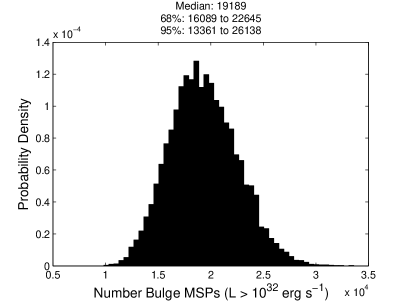
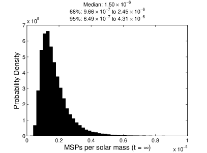
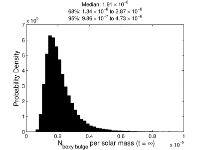
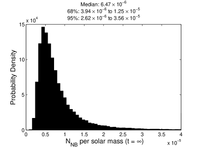
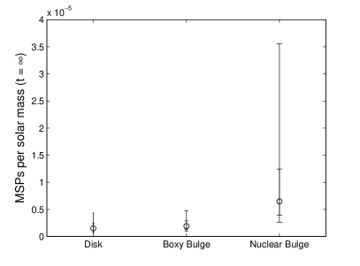
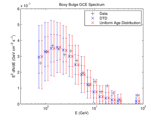
In Figs. 2, 3, and 4, we display corner plots showing some of these parameters for the best model, which was A1 which had L=ηEcutaγBbγE˙dγ𝐿𝜂superscriptsubscript𝐸cutsubscript𝑎𝛾superscript𝐵subscript𝑏𝛾superscript˙𝐸subscript𝑑𝛾L=\eta E_{\rm cut}^{a_{\gamma}}B^{b_{\gamma}}\dot{E}^{d_{\gamma}}. In Fig. 5 the resolved MSP and GCE data is compared to simulated data. We exclude data that led to an apparently negative P˙intsubscript˙𝑃int\dot{P}_{\rm int} from the binned P˙˙𝑃\dot{P} data. This exclusion affects all bins with data except the highest two. The luminosity distribution is shown in Fig. 6, and the MSP age distributions are shown in Fig. 7. In Fig. 8 we compare the total gamma ray emission from MSPs in the region of interest to the observed total. In Fig. 9 we show the number of MSPs in the disk and in the bulge. The number with luminosity greater than 1032 erg s1superscript1032superscript erg s110^{32}\textrm{ erg s}^{-1} is shown in Fig. 10, and in Fig. 11 we show the number of MSPs produced per solar mass at t=𝑡t=\infty assuming no further star formation after today. The masses used were (3.7±0.5)×1010Mplus-or-minus3.70.5superscript1010subscript𝑀direct-product(3.7\pm 0.5)\times 10^{10}{\,M_{\odot}} for the disk, (1.6±0.2)×1010Mplus-or-minus1.60.2superscript1010subscript𝑀direct-product(1.6\pm 0.2)\times 10^{10}{\,M_{\odot}} for the boxy bulge, and (1.4±0.6)×109Mplus-or-minus1.40.6superscript109subscript𝑀direct-product(1.4\pm 0.6)\times 10^{9}{\,M_{\odot}} for the nuclear bulge [38, 15]. In Fig. 12 we show the modeled probability of resolving N𝑁N bulge MSPs, as well as the number for double and quadruple the current sensitivity. In Fig. 13 we compare the posterior predictive distributions for the boxy bulge spectra in the cases where we fitted the DTD and where the MSPs were uniformly distributed in age.

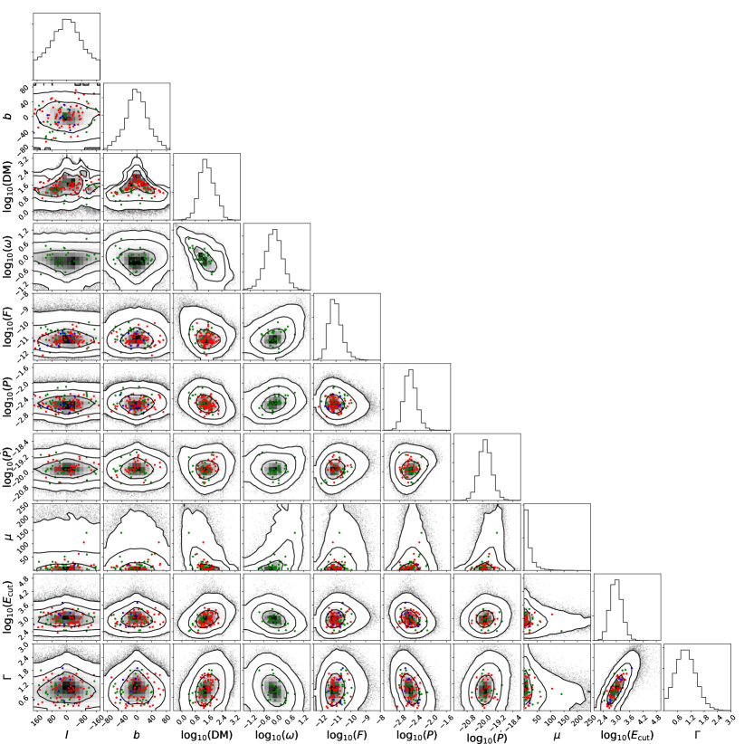
Finally, we also display corner plots showing the distributions of simulated, resolved MSPs for different models of the MSP luminosity function: Fig. 14 shows the L=ηEcutaγBbγE˙dγ𝐿𝜂superscriptsubscript𝐸cutsubscript𝑎𝛾superscript𝐵subscript𝑏𝛾superscript˙𝐸subscript𝑑𝛾L=\eta E_{\rm cut}^{a_{\gamma}}B^{b_{\gamma}}\dot{E}^{d_{\gamma}} case, Fig. 15 shows the L=η𝐿𝜂L=\eta case, and Fig. 16 shows the case for the L=ηEcutaγBbγE˙dγ𝐿𝜂superscriptsubscript𝐸cutsubscript𝑎𝛾superscript𝐵subscript𝑏𝛾superscript˙𝐸subscript𝑑𝛾L=\eta E_{\rm cut}^{a_{\gamma}}B^{b_{\gamma}}\dot{E}^{d_{\gamma}} with Ecutsubscript𝐸cutE_{\rm cut} and ΓΓ\Gamma independent of E˙˙𝐸\dot{E}.

Parameter Prior Minimum Prior Maximum
λressubscript𝜆res\lambda_{\rm res} 00 100010001000
log10(Ndisk/Nbulge)subscript10subscript𝑁disksubscript𝑁bulge\log_{10}(N_{\rm disk}/N_{\rm bulge}) 100100-100 100100100
log10(Nnb/Nbb)subscript10subscript𝑁nbsubscript𝑁bb\log_{10}(N_{\rm nb}/N_{\rm bb}) 100100-100 100100100
σrsubscript𝜎𝑟\sigma_{r} (kpc) 00 151515
z0subscript𝑧0z_{0} (kpc) 00 1.51.51.5
Kthsubscript𝐾thK_{\rm th} 2020-20 202020
σthsubscript𝜎th\sigma_{\rm th} 00 555
Cparallaxsubscript𝐶parallaxC_{\rm parallax} 00 555
log10(dparallax/kpc)subscript10subscript𝑑parallaxkpc\log_{10}(d_{\rm parallax}/{\rm kpc}) 11-1 222
aEcutsubscript𝑎subscript𝐸cuta_{E_{\rm cut}} 55-5 555
bEcutsubscript𝑏subscript𝐸cutb_{E_{\rm cut}} 222 555
σEcutsubscript𝜎subscript𝐸cut\sigma_{E_{\rm cut}} 00 333
aΓsubscript𝑎Γa_{\Gamma} 55-5 555
bΓsubscript𝑏Γb_{\Gamma} 00 555
σΓsubscript𝜎Γ\sigma_{\Gamma} 00 555
rΓ,Ecutsubscript𝑟Γsubscript𝐸cutr_{\Gamma,E_{\rm cut}} 11-1 111
aγsubscript𝑎𝛾a_{\gamma} 1010-10 101010
bγsubscript𝑏𝛾b_{\gamma} 1010-10 101010
dγsubscript𝑑𝛾d_{\gamma} 1010-10 101010
αγsubscript𝛼𝛾\alpha_{\gamma} 1010-10 101010
βγsubscript𝛽𝛾\beta_{\gamma} 1010-10 101010
DTD p(0 - 2.8 Gyr)DTD 𝑝0 - 2.8 Gyr\textrm{DTD }p(0\textrm{ - }2.8\textrm{ Gyr}) 00 111
DTD p(2.8 - 5.5 Gyr)DTD 𝑝2.8 - 5.5 Gyr\textrm{DTD }p(2.8\textrm{ - }5.5\textrm{ Gyr}) 00 111
DTD p(5.5 - 8.3 Gyr)DTD 𝑝5.5 - 8.3 Gyr\textrm{DTD }p(5.5\textrm{ - }8.3\textrm{ Gyr}) 00 111
DTD p(8.3 - 11.1 Gyr)DTD 𝑝8.3 - 11.1 Gyr\textrm{DTD }p(8.3\textrm{ - }11.1\textrm{ Gyr}) 00 111
DTD p(11.1 - 13.8 Gyr)DTD 𝑝11.1 - 13.8 Gyr\textrm{DTD }p(11.1\textrm{ - }13.8\textrm{ Gyr}) 00 111
log10(PI, med/s)subscript10subscript𝑃𝐼 meds\log_{10}(P_{I,\textrm{ med}}/\textrm{s}) 44-4 101010
σPIsubscript𝜎subscript𝑃𝐼\sigma_{P_{I}} 00 101010
CPIsubscript𝐶subscript𝑃𝐼C_{P_{I}} 22-2 555
log10(Bmed/G)subscript10subscript𝐵medG\log_{10}(B_{\rm med}/\textrm{G}) 11-1 202020
σBsubscript𝜎𝐵\sigma_{B} 00 101010
rB,PIsubscript𝑟𝐵subscript𝑃𝐼r_{B,P_{I}} 11-1 111
log10(ηmed)subscript10subscript𝜂med\log_{10}(\eta_{\rm med}) 5050-50 505050
σηsubscript𝜎𝜂\sigma_{\eta} 00 101010
σvsubscript𝜎𝑣\sigma_{v} (km s-1) 00 100001000010000
Table 1: Prior ranges for model parameters. The priors are uniform within these ranges except for the DTD bin probabilities which have a Dirichlet prior [39]. I.e. the prior for the DTD bin probabilities is uniform on a four dimensional hyperplane in the five dimensional DTD bin space. The hyperplane consist of all points for which the five DTD bin probabilities add up to one.
Model Label Description ΔWAICΔWAIC\Delta\textrm{WAIC} WAIC pWAICsubscript𝑝WAICp_{\text{WAIC}}
Std. Dev.
A1 L=ηEcutaγBbγE˙dγ𝐿𝜂superscriptsubscript𝐸cutsubscript𝑎𝛾superscript𝐵subscript𝑏𝛾superscript˙𝐸subscript𝑑𝛾L=\eta E_{\rm cut}^{a_{\gamma}}B^{b_{\gamma}}\dot{E}^{d_{\gamma}} 00 0.80.80.8 26.926.926.9
A2 L=ηEcutaγBbγE˙dγ𝐿𝜂superscriptsubscript𝐸cutsubscript𝑎𝛾superscript𝐵subscript𝑏𝛾superscript˙𝐸subscript𝑑𝛾L=\eta E_{\rm cut}^{a_{\gamma}}B^{b_{\gamma}}\dot{E}^{d_{\gamma}}, Uniform Age Distribution 0.40.40.4 1.01.01.0 26.126.126.1
A3 L=ηEcutaγBbγE˙dγ𝐿𝜂superscriptsubscript𝐸cutsubscript𝑎𝛾superscript𝐵subscript𝑏𝛾superscript˙𝐸subscript𝑑𝛾L=\eta E_{\rm cut}^{a_{\gamma}}B^{b_{\gamma}}\dot{E}^{d_{\gamma}}, Covariance B𝐵B and PIsubscript𝑃𝐼P_{I} 1.51.51.5 1.01.01.0 27.527.527.5
A4 L=ηEcutaγBbγE˙dγ𝐿𝜂superscriptsubscript𝐸cutsubscript𝑎𝛾superscript𝐵subscript𝑏𝛾superscript˙𝐸subscript𝑑𝛾L=\eta E_{\rm cut}^{a_{\gamma}}B^{b_{\gamma}}\dot{E}^{d_{\gamma}}, Eq. 2.32 Initial Period Distribution 7.37.37.3 1.51.51.5 25.925.925.9
A5 L=ηE˙αγ𝐿𝜂superscript˙𝐸subscript𝛼𝛾L=\eta\dot{E}^{\alpha_{\gamma}} 9.59.59.5 1.21.21.2 24.424.424.4
A6 L=ηPαγP˙βγ𝐿𝜂superscript𝑃subscript𝛼𝛾superscript˙𝑃subscript𝛽𝛾L=\eta P^{\alpha_{\gamma}}\dot{P}^{\beta_{\gamma}} 11.011.011.0 0.70.70.7 25.325.325.3
A7 L=ηEcutaγBbγE˙dγ𝐿𝜂superscriptsubscript𝐸cutsubscript𝑎𝛾superscript𝐵subscript𝑏𝛾superscript˙𝐸subscript𝑑𝛾L=\eta E_{\rm cut}^{a_{\gamma}}B^{b_{\gamma}}\dot{E}^{d_{\gamma}}, aEcut=aΓ=0subscript𝑎subscript𝐸cutsubscript𝑎Γ0a_{E_{\rm cut}}=a_{\Gamma}=0 19.419.419.4 0.50.50.5 25.125.125.1
A8 L=ηEcutaγBbγE˙dγ𝐿𝜂superscriptsubscript𝐸cutsubscript𝑎𝛾superscript𝐵subscript𝑏𝛾superscript˙𝐸subscript𝑑𝛾L=\eta E_{\rm cut}^{a_{\gamma}}B^{b_{\gamma}}\dot{E}^{d_{\gamma}}, aEcut=aΓ=0subscript𝑎subscript𝐸cutsubscript𝑎Γ0a_{E_{\rm cut}}=a_{\Gamma}=0, Uniform Age Distribution 21.121.121.1 0.70.70.7 24.024.024.0
A9 L=η𝐿𝜂L=\eta 42.242.242.2 0.70.70.7 24.124.124.1
B1 L=ηEcutaγBbγE˙dγ𝐿𝜂superscriptsubscript𝐸cutsubscript𝑎𝛾superscript𝐵subscript𝑏𝛾superscript˙𝐸subscript𝑑𝛾L=\eta E_{\rm cut}^{a_{\gamma}}B^{b_{\gamma}}\dot{E}^{d_{\gamma}}, Uniform Age Distribution, No GCE 00 111 242424
B2 L=ηEcutaγBbγE˙dγ𝐿𝜂superscriptsubscript𝐸cutsubscript𝑎𝛾superscript𝐵subscript𝑏𝛾superscript˙𝐸subscript𝑑𝛾L=\eta E_{\rm cut}^{a_{\gamma}}B^{b_{\gamma}}\dot{E}^{d_{\gamma}}, No GCE 1.21.21.2 0.80.80.8 25.325.325.3
B3 L=ηEcutaγBbγE˙dγ𝐿𝜂superscriptsubscript𝐸cutsubscript𝑎𝛾superscript𝐵subscript𝑏𝛾superscript˙𝐸subscript𝑑𝛾L=\eta E_{\rm cut}^{a_{\gamma}}B^{b_{\gamma}}\dot{E}^{d_{\gamma}}, Covariance B𝐵B and PIsubscript𝑃𝐼P_{I}, No GCE 2.32.32.3 0.80.80.8 26.126.126.1
B4 L=ηEcutaγBbγE˙dγ𝐿𝜂superscriptsubscript𝐸cutsubscript𝑎𝛾superscript𝐵subscript𝑏𝛾superscript˙𝐸subscript𝑑𝛾L=\eta E_{\rm cut}^{a_{\gamma}}B^{b_{\gamma}}\dot{E}^{d_{\gamma}}, Eq. 2.32 Initial Period Distribution, No GCE 999 444 242424
B5 L=ηE˙αγ𝐿𝜂superscript˙𝐸subscript𝛼𝛾L=\eta\dot{E}^{\alpha_{\gamma}}, No GCE 131313 111 232323
B6 L=ηPαγP˙βγ𝐿𝜂superscript𝑃subscript𝛼𝛾superscript˙𝑃subscript𝛽𝛾L=\eta P^{\alpha_{\gamma}}\dot{P}^{\beta_{\gamma}}, No GCE 15.215.215.2 0.90.90.9 23.823.823.8
B7 L=ηEcutaγBbγE˙dγ𝐿𝜂superscriptsubscript𝐸cutsubscript𝑎𝛾superscript𝐵subscript𝑏𝛾superscript˙𝐸subscript𝑑𝛾L=\eta E_{\rm cut}^{a_{\gamma}}B^{b_{\gamma}}\dot{E}^{d_{\gamma}}, aEcut=aΓ=0subscript𝑎subscript𝐸cutsubscript𝑎Γ0a_{E_{\rm cut}}=a_{\Gamma}=0, No GCE 21.321.321.3 0.90.90.9 23.623.623.6
B8 L=ηEcutaγBbγE˙dγ𝐿𝜂superscriptsubscript𝐸cutsubscript𝑎𝛾superscript𝐵subscript𝑏𝛾superscript˙𝐸subscript𝑑𝛾L=\eta E_{\rm cut}^{a_{\gamma}}B^{b_{\gamma}}\dot{E}^{d_{\gamma}}, aEcut=aΓ=0subscript𝑎subscript𝐸cutsubscript𝑎Γ0a_{E_{\rm cut}}=a_{\Gamma}=0, Uniform Age Distribution, No GCE 22.922.922.9 0.90.90.9 22.522.522.5
B9 L=η𝐿𝜂L=\eta, No GCE 474747 222 232323
Table 2: Average WAIC for each model relative to the model with best (lowest) WAIC. The average is taken over eight MCMC chains run for each model. We separate cases where we do not fit a GCE (B1-B9) from those where we do (A1-A9). The WAIC standard deviation column shows the sample standard deviation of WAIC for the eight MCMC chains run for each model. The pWAICsubscript𝑝WAICp_{\rm WAIC} column gives a measure of the effective number of parameters for the corresponding model [34, 33].
Parameter Model A1 Model B2 Model A5 Model A7 Model A9
λressubscript𝜆res\lambda_{\rm res} 108+11101081110108\begin{subarray}{c}+11\\ -10\end{subarray} 107+11101071110107\begin{subarray}{c}+11\\ -10\end{subarray} 108+10101081010108\begin{subarray}{c}+10\\ -10\end{subarray} 108+11101081110108\begin{subarray}{c}+11\\ -10\end{subarray} 108+11101081110108\begin{subarray}{c}+11\\ -10\end{subarray}
log10(Ndisk/Nbulge)subscript10subscript𝑁disksubscript𝑁bulge\log_{10}(N_{\rm disk}/N_{\rm bulge}) 0.00+0.130.120.000.130.120.00\begin{subarray}{c}+0.13\\ -0.12\end{subarray} - 0.00+0.130.120.000.130.120.00\begin{subarray}{c}+0.13\\ -0.12\end{subarray} 0.04+0.120.110.040.120.110.04\begin{subarray}{c}+0.12\\ -0.11\end{subarray} 0.09+0.110.100.090.110.100.09\begin{subarray}{c}+0.11\\ -0.10\end{subarray}
log10(Nnb/Nbb)subscript10subscript𝑁nbsubscript𝑁bb\log_{10}(N_{\rm nb}/N_{\rm bb}) 0.66+0.080.070.660.080.07-0.66\begin{subarray}{c}+0.08\\ -0.07\end{subarray} - 0.66+0.080.070.660.080.07-0.66\begin{subarray}{c}+0.08\\ -0.07\end{subarray} 0.61+0.060.070.610.060.07-0.61\begin{subarray}{c}+0.06\\ -0.07\end{subarray} 0.58+0.040.040.580.040.04-0.58\begin{subarray}{c}+0.04\\ -0.04\end{subarray}
σrsubscript𝜎𝑟\sigma_{r} (kpc) 4.5+0.50.44.50.50.44.5\begin{subarray}{c}+0.5\\ -0.4\end{subarray} 4.5+0.50.44.50.50.44.5\begin{subarray}{c}+0.5\\ -0.4\end{subarray} 4.4+0.50.44.40.50.44.4\begin{subarray}{c}+0.5\\ -0.4\end{subarray} 4.4+0.50.44.40.50.44.4\begin{subarray}{c}+0.5\\ -0.4\end{subarray} 4.5+0.60.44.50.60.44.5\begin{subarray}{c}+0.6\\ -0.4\end{subarray}
z0subscript𝑧0z_{0} (kpc) 0.71+0.110.090.710.110.090.71\begin{subarray}{c}+0.11\\ -0.09\end{subarray} 0.70+0.100.090.700.100.090.70\begin{subarray}{c}+0.10\\ -0.09\end{subarray} 0.71+0.110.090.710.110.090.71\begin{subarray}{c}+0.11\\ -0.09\end{subarray} 0.71+0.110.090.710.110.090.71\begin{subarray}{c}+0.11\\ -0.09\end{subarray} 0.72+0.110.090.720.110.090.72\begin{subarray}{c}+0.11\\ -0.09\end{subarray}
Kthsubscript𝐾thK_{\rm th} 0.45+0.090.080.450.090.080.45\begin{subarray}{c}+0.09\\ -0.08\end{subarray} 0.43+0.090.080.430.090.080.43\begin{subarray}{c}+0.09\\ -0.08\end{subarray} 0.45+0.090.080.450.090.080.45\begin{subarray}{c}+0.09\\ -0.08\end{subarray} 0.46+0.090.080.460.090.080.46\begin{subarray}{c}+0.09\\ -0.08\end{subarray} 0.46+0.090.080.460.090.080.46\begin{subarray}{c}+0.09\\ -0.08\end{subarray}
σthsubscript𝜎th\sigma_{\rm th} 0.28+0.050.040.280.050.040.28\begin{subarray}{c}+0.05\\ -0.04\end{subarray} 0.27+0.050.040.270.050.040.27\begin{subarray}{c}+0.05\\ -0.04\end{subarray} 0.28+0.050.040.280.050.040.28\begin{subarray}{c}+0.05\\ -0.04\end{subarray} 0.28+0.050.040.280.050.040.28\begin{subarray}{c}+0.05\\ -0.04\end{subarray} 0.28+0.050.040.280.050.040.28\begin{subarray}{c}+0.05\\ -0.04\end{subarray}
Cparallaxsubscript𝐶parallaxC_{\rm parallax} 0.43+0.150.100.430.150.100.43\begin{subarray}{c}+0.15\\ -0.10\end{subarray} 0.45+0.160.110.450.160.110.45\begin{subarray}{c}+0.16\\ -0.11\end{subarray} 0.43+0.150.100.430.150.100.43\begin{subarray}{c}+0.15\\ -0.10\end{subarray} 0.43+0.150.100.430.150.100.43\begin{subarray}{c}+0.15\\ -0.10\end{subarray} 0.40+0.130.080.400.130.080.40\begin{subarray}{c}+0.13\\ -0.08\end{subarray}
log10(dparallax/kpc)subscript10subscript𝑑parallaxkpc\log_{10}(d_{\rm parallax}/{\rm kpc}) 0.8+0.60.30.80.60.30.8\begin{subarray}{c}+0.6\\ -0.3\end{subarray} 0.7+0.60.30.70.60.30.7\begin{subarray}{c}+0.6\\ -0.3\end{subarray} 0.8+0.60.30.80.60.30.8\begin{subarray}{c}+0.6\\ -0.3\end{subarray} 0.8+0.60.30.80.60.30.8\begin{subarray}{c}+0.6\\ -0.3\end{subarray} 0.9+0.60.40.90.60.40.9\begin{subarray}{c}+0.6\\ -0.4\end{subarray}
aEcutsubscript𝑎subscript𝐸cuta_{E_{\rm cut}} 0.18+0.050.050.180.050.050.18\begin{subarray}{c}+0.05\\ -0.05\end{subarray} 0.21+0.050.050.210.050.050.21\begin{subarray}{c}+0.05\\ -0.05\end{subarray} 0.19+0.050.050.190.050.050.19\begin{subarray}{c}+0.05\\ -0.05\end{subarray} - 0.17+0.050.050.170.050.050.17\begin{subarray}{c}+0.05\\ -0.05\end{subarray}
bEcutsubscript𝑏subscript𝐸cutb_{E_{\rm cut}} 2.83+0.050.062.830.050.062.83\begin{subarray}{c}+0.05\\ -0.06\end{subarray} 2.79+0.060.072.790.060.072.79\begin{subarray}{c}+0.06\\ -0.07\end{subarray} 2.99+0.030.022.990.030.022.99\begin{subarray}{c}+0.03\\ -0.02\end{subarray} 2.79+0.060.062.790.060.062.79\begin{subarray}{c}+0.06\\ -0.06\end{subarray} 2.99+0.030.032.990.030.032.99\begin{subarray}{c}+0.03\\ -0.03\end{subarray}
σEcutsubscript𝜎subscript𝐸cut\sigma_{E_{\rm cut}} 0.23+0.020.020.230.020.020.23\begin{subarray}{c}+0.02\\ -0.02\end{subarray} 0.23+0.020.020.230.020.020.23\begin{subarray}{c}+0.02\\ -0.02\end{subarray} 0.22+0.020.020.220.020.020.22\begin{subarray}{c}+0.02\\ -0.02\end{subarray} 0.25+0.020.020.250.020.020.25\begin{subarray}{c}+0.02\\ -0.02\end{subarray} 0.23+0.020.020.230.020.020.23\begin{subarray}{c}+0.02\\ -0.02\end{subarray}
aΓsubscript𝑎Γa_{\Gamma} 0.41+0.080.080.410.080.080.41\begin{subarray}{c}+0.08\\ -0.08\end{subarray} 0.43+0.080.080.430.080.080.43\begin{subarray}{c}+0.08\\ -0.08\end{subarray} 0.43+0.070.080.430.070.080.43\begin{subarray}{c}+0.07\\ -0.08\end{subarray} - 0.39+0.080.080.390.080.080.39\begin{subarray}{c}+0.08\\ -0.08\end{subarray}
bΓsubscript𝑏Γb_{\Gamma} 0.81+0.070.080.810.070.080.81\begin{subarray}{c}+0.07\\ -0.08\end{subarray} 0.77+0.080.100.770.080.100.77\begin{subarray}{c}+0.08\\ -0.10\end{subarray} 1.00+0.040.041.000.040.041.00\begin{subarray}{c}+0.04\\ -0.04\end{subarray} 0.70+0.090.100.700.090.100.70\begin{subarray}{c}+0.09\\ -0.10\end{subarray} 0.99+0.040.040.990.040.040.99\begin{subarray}{c}+0.04\\ -0.04\end{subarray}
σΓsubscript𝜎Γ\sigma_{\Gamma} 0.36+0.040.030.360.040.030.36\begin{subarray}{c}+0.04\\ -0.03\end{subarray} 0.36+0.040.030.360.040.030.36\begin{subarray}{c}+0.04\\ -0.03\end{subarray} 0.34+0.030.030.340.030.030.34\begin{subarray}{c}+0.03\\ -0.03\end{subarray} 0.42+0.040.030.420.040.030.42\begin{subarray}{c}+0.04\\ -0.03\end{subarray} 0.35+0.030.030.350.030.030.35\begin{subarray}{c}+0.03\\ -0.03\end{subarray}
rΓ,Ecutsubscript𝑟Γsubscript𝐸cutr_{\Gamma,E_{\rm cut}} 0.75+0.050.060.750.050.060.75\begin{subarray}{c}+0.05\\ -0.06\end{subarray} 0.77+0.050.060.770.050.060.77\begin{subarray}{c}+0.05\\ -0.06\end{subarray} 0.73+0.060.070.730.060.070.73\begin{subarray}{c}+0.06\\ -0.07\end{subarray} 0.79+0.040.050.790.040.050.79\begin{subarray}{c}+0.04\\ -0.05\end{subarray} 0.75+0.050.060.750.050.060.75\begin{subarray}{c}+0.05\\ -0.06\end{subarray}
aγsubscript𝑎𝛾a_{\gamma} 1.2+0.30.31.20.30.31.2\begin{subarray}{c}+0.3\\ -0.3\end{subarray} 1.4+0.30.31.40.30.31.4\begin{subarray}{c}+0.3\\ -0.3\end{subarray} - 1.3+0.30.31.30.30.31.3\begin{subarray}{c}+0.3\\ -0.3\end{subarray} -
bγsubscript𝑏𝛾b_{\gamma} 0.1+0.40.40.10.40.40.1\begin{subarray}{c}+0.4\\ -0.4\end{subarray} 0.1+0.40.40.10.40.40.1\begin{subarray}{c}+0.4\\ -0.4\end{subarray} - 0.1+0.40.40.10.40.40.1\begin{subarray}{c}+0.4\\ -0.4\end{subarray} -
dγsubscript𝑑𝛾d_{\gamma} 0.50+0.120.120.500.120.120.50\begin{subarray}{c}+0.12\\ -0.12\end{subarray} 0.48+0.120.120.480.120.120.48\begin{subarray}{c}+0.12\\ -0.12\end{subarray} - 0.56+0.110.100.560.110.100.56\begin{subarray}{c}+0.11\\ -0.10\end{subarray} -
αγsubscript𝛼𝛾\alpha_{\gamma} - - 0.74+0.110.100.740.110.100.74\begin{subarray}{c}+0.11\\ -0.10\end{subarray} - -
DTD p(0 - 2.8 Gyr)DTD 𝑝0 - 2.8 Gyr\textrm{DTD }p(0\textrm{ - }2.8\textrm{ Gyr}) 0.13+0.140.090.130.140.090.13\begin{subarray}{c}+0.14\\ -0.09\end{subarray} 0.13+0.150.090.130.150.090.13\begin{subarray}{c}+0.15\\ -0.09\end{subarray} 0.13+0.140.090.130.140.090.13\begin{subarray}{c}+0.14\\ -0.09\end{subarray} 0.10+0.110.070.100.110.070.10\begin{subarray}{c}+0.11\\ -0.07\end{subarray} 0.02+0.020.010.020.020.010.02\begin{subarray}{c}+0.02\\ -0.01\end{subarray}
DTD p(2.8 - 5.5 Gyr)DTD 𝑝2.8 - 5.5 Gyr\textrm{DTD }p(2.8\textrm{ - }5.5\textrm{ Gyr}) 0.15+0.180.110.150.180.110.15\begin{subarray}{c}+0.18\\ -0.11\end{subarray} 0.15+0.190.110.150.190.110.15\begin{subarray}{c}+0.19\\ -0.11\end{subarray} 0.15+0.180.110.150.180.110.15\begin{subarray}{c}+0.18\\ -0.11\end{subarray} 0.12+0.160.090.120.160.090.12\begin{subarray}{c}+0.16\\ -0.09\end{subarray} 0.02+0.030.020.020.030.020.02\begin{subarray}{c}+0.03\\ -0.02\end{subarray}
DTD p(5.5 - 8.3 Gyr)DTD 𝑝5.5 - 8.3 Gyr\textrm{DTD }p(5.5\textrm{ - }8.3\textrm{ Gyr}) 0.29+0.200.170.290.200.170.29\begin{subarray}{c}+0.20\\ -0.17\end{subarray} 0.26+0.180.160.260.180.160.26\begin{subarray}{c}+0.18\\ -0.16\end{subarray} 0.29+0.200.170.290.200.170.29\begin{subarray}{c}+0.20\\ -0.17\end{subarray} 0.25+0.180.140.250.180.140.25\begin{subarray}{c}+0.18\\ -0.14\end{subarray} 0.09+0.060.050.090.060.050.09\begin{subarray}{c}+0.06\\ -0.05\end{subarray}
DTD p(8.3 - 11.1 Gyr)DTD 𝑝8.3 - 11.1 Gyr\textrm{DTD }p(8.3\textrm{ - }11.1\textrm{ Gyr}) 0.14+0.160.100.140.160.100.14\begin{subarray}{c}+0.16\\ -0.10\end{subarray} 0.11+0.140.080.110.140.080.11\begin{subarray}{c}+0.14\\ -0.08\end{subarray} 0.15+0.170.100.150.170.100.15\begin{subarray}{c}+0.17\\ -0.10\end{subarray} 0.14+0.170.100.140.170.100.14\begin{subarray}{c}+0.17\\ -0.10\end{subarray} 0.06+0.110.050.060.110.050.06\begin{subarray}{c}+0.11\\ -0.05\end{subarray}
DTD p(11.1 - 13.8 Gyr)DTD 𝑝11.1 - 13.8 Gyr\textrm{DTD }p(11.1\textrm{ - }13.8\textrm{ Gyr}) 0.14+0.220.110.140.220.110.14\begin{subarray}{c}+0.22\\ -0.11\end{subarray} 0.22+0.200.150.220.200.150.22\begin{subarray}{c}+0.20\\ -0.15\end{subarray} 0.13+0.210.100.130.210.100.13\begin{subarray}{c}+0.21\\ -0.10\end{subarray} 0.27+0.240.190.270.240.190.27\begin{subarray}{c}+0.24\\ -0.19\end{subarray} 0.78+0.080.140.780.080.140.78\begin{subarray}{c}+0.08\\ -0.14\end{subarray}
log10(Pi, med/s)subscript10subscript𝑃𝑖 meds\log_{10}(P_{i,\textrm{ med}}/\textrm{s}) 2.61+0.050.042.610.050.04-2.61\begin{subarray}{c}+0.05\\ -0.04\end{subarray} 2.60+0.050.042.600.050.04-2.60\begin{subarray}{c}+0.05\\ -0.04\end{subarray} 2.61+0.050.042.610.050.04-2.61\begin{subarray}{c}+0.05\\ -0.04\end{subarray} 2.63+0.040.032.630.040.03-2.63\begin{subarray}{c}+0.04\\ -0.03\end{subarray} 2.69+0.030.032.690.030.03-2.69\begin{subarray}{c}+0.03\\ -0.03\end{subarray}
σPisubscript𝜎subscript𝑃𝑖\sigma_{P_{i}} 0.13+0.020.020.130.020.020.13\begin{subarray}{c}+0.02\\ -0.02\end{subarray} 0.13+0.020.020.130.020.020.13\begin{subarray}{c}+0.02\\ -0.02\end{subarray} 0.13+0.020.020.130.020.020.13\begin{subarray}{c}+0.02\\ -0.02\end{subarray} 0.12+0.020.020.120.020.020.12\begin{subarray}{c}+0.02\\ -0.02\end{subarray} 0.13+0.020.020.130.020.020.13\begin{subarray}{c}+0.02\\ -0.02\end{subarray}
log10(Bmed/G)subscript10subscript𝐵medG\log_{10}(B_{\rm med}/\textrm{G}) 8.21+0.050.068.210.050.068.21\begin{subarray}{c}+0.05\\ -0.06\end{subarray} 8.21+0.060.068.210.060.068.21\begin{subarray}{c}+0.06\\ -0.06\end{subarray} 8.21+0.030.048.210.030.048.21\begin{subarray}{c}+0.03\\ -0.04\end{subarray} 8.21+0.050.058.210.050.058.21\begin{subarray}{c}+0.05\\ -0.05\end{subarray} 8.25+0.020.028.250.020.028.25\begin{subarray}{c}+0.02\\ -0.02\end{subarray}
σBsubscript𝜎𝐵\sigma_{B} 0.21+0.030.020.210.030.020.21\begin{subarray}{c}+0.03\\ -0.02\end{subarray} 0.21+0.030.020.210.030.020.21\begin{subarray}{c}+0.03\\ -0.02\end{subarray} 0.22+0.030.030.220.030.030.22\begin{subarray}{c}+0.03\\ -0.03\end{subarray} 0.21+0.030.030.210.030.030.21\begin{subarray}{c}+0.03\\ -0.03\end{subarray} 0.19+0.020.020.190.020.020.19\begin{subarray}{c}+0.02\\ -0.02\end{subarray}
log10(ηmed)subscript10subscript𝜂med\log_{10}(\eta_{\rm med}) 12+55125512\begin{subarray}{c}+5\\ -5\end{subarray} 12+55125512\begin{subarray}{c}+5\\ -5\end{subarray} 7+447447\begin{subarray}{c}+4\\ -4\end{subarray} 9+449449\begin{subarray}{c}+4\\ -4\end{subarray} 32.17+0.230.3132.170.230.3132.17\begin{subarray}{c}+0.23\\ -0.31\end{subarray}
σηsubscript𝜎𝜂\sigma_{\eta} 0.52+0.060.050.520.060.050.52\begin{subarray}{c}+0.06\\ -0.05\end{subarray} 0.53+0.060.050.530.060.050.53\begin{subarray}{c}+0.06\\ -0.05\end{subarray} 0.58+0.060.050.580.060.050.58\begin{subarray}{c}+0.06\\ -0.05\end{subarray} 0.51+0.060.050.510.060.050.51\begin{subarray}{c}+0.06\\ -0.05\end{subarray} 0.72+0.080.060.720.080.060.72\begin{subarray}{c}+0.08\\ -0.06\end{subarray}
σvsubscript𝜎𝑣\sigma_{v} (km s-1) 77+66776677\begin{subarray}{c}+6\\ -6\end{subarray} 76+65766576\begin{subarray}{c}+6\\ -5\end{subarray} 77+66776677\begin{subarray}{c}+6\\ -6\end{subarray} 77+66776677\begin{subarray}{c}+6\\ -6\end{subarray} 78+66786678\begin{subarray}{c}+6\\ -6\end{subarray}
Table 3: Medians and 68%percent6868\% confidence intervals for a selection of different models of the Galactic MSP population. See Table 2 for a description of the model labels.
Refer to caption
Figure 2: Corner plot showing a selection of parameters for Model A1 (L=ηEcutaγBbγE˙dγ𝐿𝜂superscriptsubscript𝐸cutsubscript𝑎𝛾superscript𝐵subscript𝑏𝛾superscript˙𝐸subscript𝑑𝛾L=\eta E_{\rm cut}^{a_{\gamma}}B^{b_{\gamma}}\dot{E}^{d_{\gamma}}) with 68%percent6868\% and 95%percent9595\% contours. These parameters relate to the luminosity, Ecutsubscript𝐸cutE_{\rm cut}, ΓΓ\Gamma and B𝐵B distributions. The Bmedsubscript𝐵medB_{\rm med} parameter has units of Gauss.
Refer to caption
Figure 3: Corner plot showing a selection of parameters for Model A1 with 68%percent6868\% and 95%percent9595\% contours. These parameters relate to the number of MSPs in different components of the spatial distribution, the flux threshold, the model of the parallax measurement availability and the initial period distribution. The parameters σrsubscript𝜎𝑟\sigma_{r}, z0subscript𝑧0z_{0}, and dparallaxsubscript𝑑parallaxd_{\rm parallax} have units of kpc.
Refer to caption
Figure 4: Model A1 probability of delay time within each DTD bin.
Refer to caption
Refer to caption
Refer to caption
Refer to caption
Refer to caption
Refer to caption
Refer to caption
Refer to caption
Refer to caption
Refer to caption
Refer to caption
Refer to caption
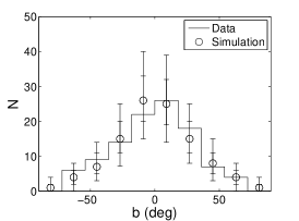
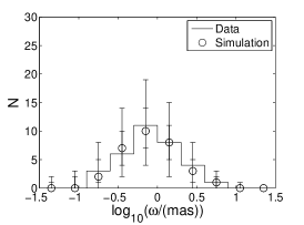
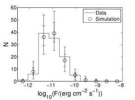
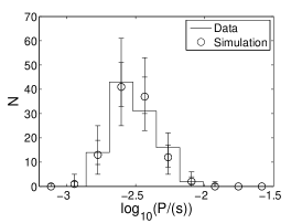
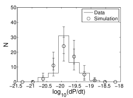
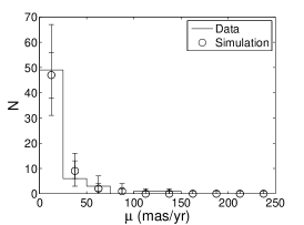
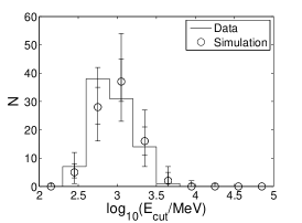
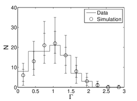
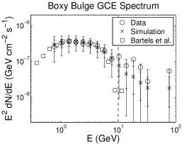
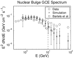
Figure 5: Observed data compared to simulated observations for Model A1 of longitude l𝑙l (deg), latitude b𝑏b (deg), dispersion measure DM (cm-3 pc), parallax ω𝜔\omega (mas), flux F𝐹F (erg cm-2 s-1), period P𝑃P (s), period derivative P˙˙𝑃\dot{P}, proper motion μ𝜇\mu (mas yr-1), spectral cutoff Ecutsubscript𝐸cutE_{\rm cut} (MeV), spectral index ΓΓ\Gamma and GCE spectra for the boxy and nuclear bulges. The GCE spectra are for the inner 40×40superscript40superscript4040^{\circ}\times 40^{\circ} region and the vertical dashed line shows the energy up to which we fitted of 101010 GeV. The simulated data is shown as medians, 68%percent6868\% and 95%percent9595\% intervals in each bin. The intervals on the simulated GCE data include the errors on the observed data. For the GCE plots, we also show boxy bulge and nuclear bulge spectra from Bartels et al. [6] in addition to those we fitted to of Macias et al. [7].
Refer to caption
Refer to caption
Refer to caption
Figure 6: MSP luminosity distribution in the disk and the change in probability density for the boxy bulge and nuclear bulge for Model A1. The black line shows the median probability density in each bin, dark grey the 68%percent6868\% interval and light grey the 95%percent9595\% interval. Note that the probability density is of log10(L/(ergs1))subscript10𝐿ergsuperscripts1\log_{10}(L/({\rm erg\,s^{-1}})) rather than of L/(ergs1)𝐿ergsuperscripts1L/({\rm erg\,s^{-1}}).
Refer to caption
Refer to caption
Refer to caption
Figure 7: MSP age distribution in the disk, boxy bulge and nuclear bulge for Model A1. The black line shows the median probability density in each bin, dark grey the 68%percent6868\% interval and light grey the 95%percent9595\% interval.
Refer to caption
Figure 8: Total observed gamma ray emission compared to all simulated MSP emission from inner 40×40superscript40superscript4040^{\circ}\times 40^{\circ} region for Model A1. Data is from Abazajian et al. [8].
Refer to caption
Refer to caption
Figure 9: Distribution of the number of disk and bulge MSPs for Model A1.
Refer to caption
Refer to caption
Figure 10: Distribution of the number of disk and bulge MSPs with L>1032 erg s1𝐿superscript1032superscript erg s1L>10^{32}\textrm{ erg s}^{-1} for Model A1.
Refer to caption
Refer to caption
Refer to caption
Refer to caption
Figure 11: Distribution of the number of disk, boxy bulge and nuclear bulge MSPs produced per solar mass at t=𝑡t=\infty assuming no further star formation beyond today for Model A1. In the bottom right plot, the medians, 68%percent6868\% and 95%percent9595\% intervals are shown side by side.
Refer to caption
Refer to caption
Refer to caption
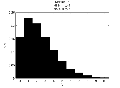
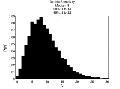
Figure 12: Probability of observing N𝑁N bulge MSPs with the current sensitivity as well as for two and four times the current sensitivity for Model A1. The double and quadruple sensitivity distributions were produced by subtracting 0.30.30.3 and 0.60.60.6 respectively from Kthsubscript𝐾thK_{\rm th}.
Refer to caption
Figure 13: Comparison of posterior predictive boxy bulge GCE spectra for the L=ηEcutaγBbγE˙dγ𝐿𝜂superscriptsubscript𝐸cutsubscript𝑎𝛾superscript𝐵subscript𝑏𝛾superscript˙𝐸subscript𝑑𝛾L=\eta E_{\rm cut}^{a_{\gamma}}B^{b_{\gamma}}\dot{E}^{d_{\gamma}} model in the case where we have a DTD (Model A1) and the case where a uniform MSP age distribution was used (Model A2). The DTD case has been shifted slightly to the left and the uniform case to the right in order to make comparison easier. Only bins with E<10𝐸10E<10 GeV were fitted.
Refer to caption
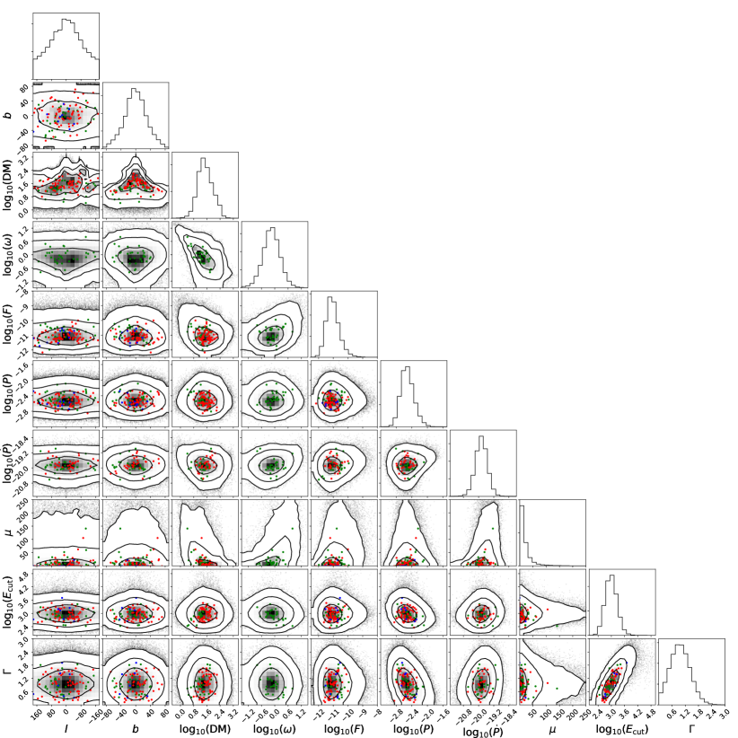
Figure 14: Model A1 (L=ηEcutaγBbγE˙dγ𝐿𝜂superscriptsubscript𝐸cutsubscript𝑎𝛾superscript𝐵subscript𝑏𝛾superscript˙𝐸subscript𝑑𝛾L=\eta E_{\rm cut}^{a_{\gamma}}B^{b_{\gamma}}\dot{E}^{d_{\gamma}}) posterior predictive corner plots showing longitude l𝑙l (deg), latitude b𝑏b (deg), dispersion measure DM (cm-3 pc), parallax ω𝜔\omega (mas), flux F𝐹F (erg cm-2 s-1), period P𝑃P (s), period derivative P˙˙𝑃\dot{P}, proper motion μ𝜇\mu (mas yr-1), spectral cutoff Ecutsubscript𝐸cutE_{\rm cut} (MeV) and spectral index ΓΓ\Gamma simulated and real data. Red points are MSPs with dispersion measure distances, green is parallax, and blue is no distance measurement. The contours show regions containing 68%percent6868\%, 95%percent9595\% and 99.7%percent99.799.7\% of the simulated data.
Refer to caption
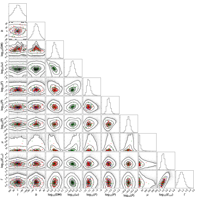
Figure 15: The same as Fig. 14 except for Model A9 which has L=η𝐿𝜂L=\eta.
Refer to caption
Figure 16: The same as Fig. 14 except for Model A7 which has the same luminosity function as Model A1 but has Ecutsubscript𝐸cutE_{\rm cut} independent of E˙˙𝐸\dot{E} (aEcut=aΓ=0subscript𝑎subscript𝐸cutsubscript𝑎Γ0a_{E_{\rm cut}}=a_{\Gamma}=0).

4 Discussion
Refer to caption
Refer to caption
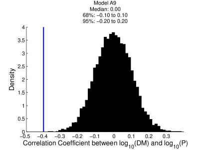
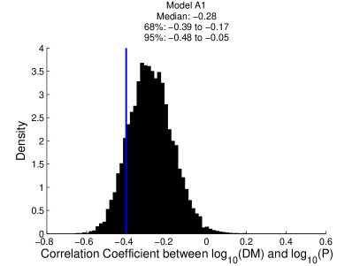
Figure 17: Comparison of correlation coefficients between log10(P)subscript10𝑃\log_{10}(P) and log10(DM)subscript10DM\log_{10}({\rm DM}) for resolved MSP simulated and real data for Model A1 (L=ηEcutaγBbγE˙dγ𝐿𝜂superscriptsubscript𝐸cutsubscript𝑎𝛾superscript𝐵subscript𝑏𝛾superscript˙𝐸subscript𝑑𝛾L=\eta E_{\rm cut}^{a_{\gamma}}B^{b_{\gamma}}\dot{E}^{d_{\gamma}}) on the left and Model A9 (L=η𝐿𝜂L=\eta) on the right. The blue line shows the correlation coefficient for the resolved MSP data at -0.40. The posterior predictive p-values are 0.130.130.13 for A1, and 00 for A9.
log10(ω)subscript10𝜔\log_{10}(\omega) 0.4170.4170.417
log10(F)subscript10𝐹\log_{10}(F) 0.6270.6270.627 0.1590.1590.159
log10(P)subscript10𝑃\log_{10}(P) 0.1260.1260.126 0.9480.9480.948 0.7520.7520.752
log10(P˙)subscript10˙𝑃\log_{10}(\dot{P}) 0.9110.9110.911 0.2450.2450.245 0.4510.4510.451 0.1590.1590.159
μ𝜇\mu 0.0340.0340.034 0.3980.3980.398 0.2940.2940.294 0.9380.9380.938 0.3380.3380.338
log10(Ecut)subscript10subscript𝐸cut\log_{10}(E_{\rm cut}) 0.7890.7890.789 0.0390.0390.039 0.4370.4370.437 0.5270.5270.527 0.3820.3820.382 0.4770.4770.477
ΓΓ\Gamma 0.5500.5500.550 0.1630.1630.163 0.7730.7730.773 0.5830.5830.583 0.3520.3520.352 0.7070.7070.707 0.6120.6120.612
log10(DM)subscript10DM\log_{10}(\textrm{DM}) log10(ω)subscript10𝜔\log_{10}(\omega) log10(F)subscript10𝐹\log_{10}(F) log10(P)subscript10𝑃\log_{10}(P) log10(P˙)subscript10˙𝑃\log_{10}(\dot{P}) μ𝜇\mu log10(Ecut)subscript10subscript𝐸cut\log_{10}(E_{\rm cut})
Table 4: Posterior predictive p-values for the correlation coefficients between observables for Model A1 which has L=ηEcutaγBbγE˙dγ𝐿𝜂superscriptsubscript𝐸cutsubscript𝑎𝛾superscript𝐵subscript𝑏𝛾superscript˙𝐸subscript𝑑𝛾L=\eta E_{\rm cut}^{a_{\gamma}}B^{b_{\gamma}}\dot{E}^{d_{\gamma}}.
log10(ω)subscript10𝜔\log_{10}(\omega) 0.4260.4260.426
log10(F)subscript10𝐹\log_{10}(F) 0.6150.6150.615 0.1580.1580.158
log10(P)subscript10𝑃\log_{10}(P) 0.1380.1380.138 0.9410.9410.941 0.7430.7430.743
log10(P˙)subscript10˙𝑃\log_{10}(\dot{P}) 0.8910.8910.891 0.2650.2650.265 0.4310.4310.431 0.1450.1450.145
μ𝜇\mu 0.4300.4300.430 0.3950.3950.395 0.2820.2820.282 0.9320.9320.932 0.3660.3660.366
log10(Ecut)subscript10subscript𝐸cut\log_{10}(E_{\rm cut}) 0.9920.992{\color[rgb]{1,0,0}\definecolor[named]{pgfstrokecolor}{rgb}{1,0,0}0.992} 0.0070.007{\color[rgb]{1,0,0}\definecolor[named]{pgfstrokecolor}{rgb}{1,0,0}0.007} 0.6970.6970.697 0.6090.6090.609 0.2160.2160.216 0.1750.1750.175
ΓΓ\Gamma 0.8520.8520.852 0.0690.0690.069 0.8790.8790.879 0.6670.6670.667 0.2230.2230.223 0.5150.5150.515 0.6250.6250.625
log10(DM)subscript10DM\log_{10}(\textrm{DM}) log10(ω)subscript10𝜔\log_{10}(\omega) log10(F)subscript10𝐹\log_{10}(F) log10(P)subscript10𝑃\log_{10}(P) log10(P˙)subscript10˙𝑃\log_{10}(\dot{P}) μ𝜇\mu log10(Ecut)subscript10subscript𝐸cut\log_{10}(E_{\rm cut})
Table 5: Posterior predictive p-values for the correlation coefficients between observables for Model A6 which has L=ηPαγP˙βγ𝐿𝜂superscript𝑃subscript𝛼𝛾superscript˙𝑃subscript𝛽𝛾L=\eta P^{\alpha_{\gamma}}\dot{P}^{\beta_{\gamma}}. Values greater than 0.99 and less than 0.01 are marked in red.
log10(ω)subscript10𝜔\log_{10}(\omega) 0.3840.3840.384
log10(F)subscript10𝐹\log_{10}(F) 0.7190.7190.719 0.1200.1200.120
log10(P)subscript10𝑃\log_{10}(P) 0.0570.0570.057 0.9650.9650.965 0.6460.6460.646
log10(P˙)subscript10˙𝑃\log_{10}(\dot{P}) 0.9380.9380.938 0.2250.2250.225 0.5020.5020.502 0.1570.1570.157
μ𝜇\mu 0.4120.4120.412 0.4150.4150.415 0.2440.2440.244 0.9630.9630.963 0.3160.3160.316
log10(Ecut)subscript10subscript𝐸cut\log_{10}(E_{\rm cut}) 0.9420.9420.942 0.0170.0170.017 0.5830.5830.583 0.0040.004{\color[rgb]{1,0,0}\definecolor[named]{pgfstrokecolor}{rgb}{1,0,0}0.004} 0.8190.8190.819 0.3390.3390.339
ΓΓ\Gamma 0.8890.8890.889 0.0590.0590.059 0.9060.9060.906 0.0000.000\bf{\color[rgb]{1,0,0}\definecolor[named]{pgfstrokecolor}{rgb}{1,0,0}0.000} 0.8940.8940.894 0.5090.5090.509 0.6610.6610.661
log10(DM)subscript10DM\log_{10}(\textrm{DM}) log10(ω)subscript10𝜔\log_{10}(\omega) log10(F)subscript10𝐹\log_{10}(F) log10(P)subscript10𝑃\log_{10}(P) log10(P˙)subscript10˙𝑃\log_{10}(\dot{P}) μ𝜇\mu log10(Ecut)subscript10subscript𝐸cut\log_{10}(E_{\rm cut})
Table 6: Same as Table 5 except for Model A7 which has L=ηEcutaγBbγE˙dγ𝐿𝜂superscriptsubscript𝐸cutsubscript𝑎𝛾superscript𝐵subscript𝑏𝛾superscript˙𝐸subscript𝑑𝛾L=\eta E_{\rm cut}^{a_{\gamma}}B^{b_{\gamma}}\dot{E}^{d_{\gamma}}, aEcut=aΓ=0subscript𝑎subscript𝐸cutsubscript𝑎Γ0a_{E_{\rm cut}}=a_{\Gamma}=0.
log10(ω)subscript10𝜔\log_{10}(\omega) 0.4220.4220.422
log10(F)subscript10𝐹\log_{10}(F) 0.6700.6700.670 0.1410.1410.141
log10(P)subscript10𝑃\log_{10}(P) 0.0000.000\bf{\color[rgb]{1,0,0}\definecolor[named]{pgfstrokecolor}{rgb}{1,0,0}0.000} 0.9980.998{\color[rgb]{1,0,0}\definecolor[named]{pgfstrokecolor}{rgb}{1,0,0}0.998} 0.2890.2890.289
log10(P˙)subscript10˙𝑃\log_{10}(\dot{P}) 0.9970.997{\color[rgb]{1,0,0}\definecolor[named]{pgfstrokecolor}{rgb}{1,0,0}0.997} 0.1040.1040.104 0.6970.6970.697 0.1400.1400.140
μ𝜇\mu 0.4240.4240.424 0.3960.3960.396 0.2750.2750.275 0.9980.998{\color[rgb]{1,0,0}\definecolor[named]{pgfstrokecolor}{rgb}{1,0,0}0.998} 0.1550.1550.155
log10(Ecut)subscript10subscript𝐸cut\log_{10}(E_{\rm cut}) 1.0001.000{\bf{\color[rgb]{1,0,0}\definecolor[named]{pgfstrokecolor}{rgb}{1,0,0}1.000}} 0.0020.002{\color[rgb]{1,0,0}\definecolor[named]{pgfstrokecolor}{rgb}{1,0,0}0.002} 0.8690.8690.869 0.5410.5410.541 0.3160.3160.316 0.0530.0530.053
ΓΓ\Gamma 0.9980.998{\color[rgb]{1,0,0}\definecolor[named]{pgfstrokecolor}{rgb}{1,0,0}0.998} 0.0120.0120.012 0.9780.9780.978 0.6210.6210.621 0.3540.3540.354 0.1920.1920.192 0.6310.6310.631
log10(DM)subscript10DM\log_{10}(\textrm{DM}) log10(ω)subscript10𝜔\log_{10}(\omega) log10(F)subscript10𝐹\log_{10}(F) log10(P)subscript10𝑃\log_{10}(P) log10(P˙)subscript10˙𝑃\log_{10}(\dot{P}) μ𝜇\mu log10(Ecut)subscript10subscript𝐸cut\log_{10}(E_{\rm cut})
Table 7: Same as Table 5 except for Model A9 which has L=η𝐿𝜂L=\eta.

Some of our luminosity functions are nested. We can go from Model A1 with L=ηEcutaγBbγE˙dγ𝐿𝜂superscriptsubscript𝐸cutsubscript𝑎𝛾superscript𝐵subscript𝑏𝛾superscript˙𝐸subscript𝑑𝛾L=\eta E_{\rm cut}^{a_{\gamma}}B^{b_{\gamma}}\dot{E}^{d_{\gamma}} to Model A9 with L=η𝐿𝜂L=\eta by setting aγ=bγ=dγ=0subscript𝑎𝛾subscript𝑏𝛾subscript𝑑𝛾0a_{\gamma}=b_{\gamma}=d_{\gamma}=0. As can be seen from the Model A1 fit in Fig. 2 and Table 3, the data prefer the aγ=1.2±0.3subscript𝑎𝛾plus-or-minus1.20.3a_{\gamma}=1.2\pm 0.3 and dγ=0.5±0.1subscript𝑑𝛾plus-or-minus0.50.1d_{\gamma}=0.5\pm 0.1 parameters to be larger than zero at high significance. This is consistent with the results of Table 2 where Model A9 has a ΔWAIC=42.2ΔWAIC42.2\Delta{\rm WAIC}=42.2 relative to Model A1. Comparing the posterior predictive corner plots for Model A1 in Fig. 14 and Model A9 in Fig. 15 we can see that Model A9 does not capture some of the correlations in the data, particularly those between distance (shown indirectly in the form of dispersion measure) and the spectral parameter Ecutsubscript𝐸cutE_{\rm cut} as well as between distance and period. A comparison of correlation coefficients between the real data and simulated data is shown in Fig. 17. More detail can be seen by comparing Tables 4 and 7 which list the posterior predictive p-values for the correlations between observables for Models A1 and A9 respectively. Following the recommendation given in Section 6.3 of ref. [33], we consider posterior predictive p-values below 1% and above 99% to be of concern. As can be seen, the posterior predictive p-values for Model A1 are all comfortably within the 1% to 99% interval. In contrast to this, seven correlation coefficients for Model A9 are outside this interval. The correlation coefficient between log10(P)subscript10𝑃\log_{10}(P) and log10(DM)subscript10DM\log_{10}({\rm DM}) and also the one between log10(Ecut)subscript10subscript𝐸cut\log_{10}(E_{\rm cut}) and log10(DM)subscript10DM\log_{10}({\rm DM}) are both particularly discrepant with the data. These logarithmic correlations are associated with the flux threshold which implies that, the more distant the MSP, the larger the intrinsic luminosity it is required to have in order to have a significant probability of being resolved. The point distinguishing Model A1 from Model A9 in regards to the relationship between distance and Ecutsubscript𝐸cutE_{\rm cut} arises because of Model A1 having a significant positive aγ=1.2±0.3subscript𝑎𝛾plus-or-minus1.20.3a_{\gamma}=1.2\pm 0.3 in Eq. 2.24, while in Model A9 we have set aγ=0subscript𝑎𝛾0a_{\gamma}=0. Regarding the logarithmic correlation between distance and P𝑃P, it follows from the presence of P𝑃P in the denominator of Eq. 2.17 that the significantly positive dγ=0.5±0.1subscript𝑑𝛾plus-or-minus0.50.1d_{\gamma}=0.5\pm 0.1 in Eq. 2.24 leads to the negative correlation with the distance measures in Model A1, while, again, in Model A9 we have dγ=0subscript𝑑𝛾0d_{\gamma}=0 by construction.

Model A6 is related to model A1 as follows from Eqs. 2.17 and 2.18 which demonstrate that we can go from the luminosity function in Model A1 to the luminosity function in Model A6 by setting bγ=αγ2+3βγ2subscript𝑏𝛾subscript𝛼𝛾23subscript𝛽𝛾2b_{\gamma}=\frac{\alpha_{\gamma}}{2}+\frac{3\beta_{\gamma}}{2} and dγ=βγ4αγ4subscript𝑑𝛾subscript𝛽𝛾4subscript𝛼𝛾4d_{\gamma}=\frac{\beta_{\gamma}}{4}-\frac{\alpha_{\gamma}}{4}. However, Model A6 does not have a dependence on Ecutsubscript𝐸cutE_{\rm cut} and therefore assumes aγ=0subscript𝑎𝛾0a_{\gamma}=0. As can be see from Table 3, aγ=1.2±0.3subscript𝑎𝛾plus-or-minus1.20.3a_{\gamma}=1.2\pm 0.3 is significantly positive for Model A1 and so Model A1 is preferred over Model A6. This is consistent with Model A6 having a ΔWAIC=11.0ΔWAIC11.0\Delta{\rm WAIC=}11.0 relative to Model A1. As can be seen from Table 5 the problem with Model A6 is that it does not predict the observed logarithmic correlation between distance and Ecutsubscript𝐸cutE_{\rm cut}.

Model A7 is the same as Model A1 except that we set aEcut=aΓ=0subscript𝑎subscript𝐸cutsubscript𝑎Γ0a_{E_{\rm cut}}=a_{\Gamma}=0. We see from Table 3 that this choice for Model A7 is disfavoured as we found that Model A1 had a significantly positive aΓ=0.41±0.08subscript𝑎Γplus-or-minus0.410.08a_{\Gamma}=0.41\pm 0.08 for Eq. 2.29. This preference for Model A1 over A7 is confirmed in Table 2 where it can be seen that Model A7 has a ΔWAIC=19.4ΔWAIC19.4\Delta{\rm WAIC}=19.4 relative to Model A1. We can see how Model A7 produced a worse fit to the data by comparing Figs. 14 and 16: in the latter case where aEcut=aΓ=0subscript𝑎subscript𝐸cutsubscript𝑎Γ0a_{E_{\rm cut}}=a_{\Gamma}=0, the relationship between spectral index and period has clearly disappeared. This is confirmed in Table 6 where two of the correlation coefficients are of concern and, in particular, the correlation coefficient between ΓΓ\Gamma and log10(P)subscript10𝑃\log_{\rm 10}(P) has a posterior predictive p-value of 0.000.

Our best fitting model of the Galactic MSP population was Model A1 for which L=ηEcutaγBbγE˙dγ𝐿𝜂superscriptsubscript𝐸cutsubscript𝑎𝛾superscript𝐵subscript𝑏𝛾superscript˙𝐸subscript𝑑𝛾L=\eta E_{\rm cut}^{a_{\gamma}}B^{b_{\gamma}}\dot{E}^{d_{\gamma}}. From inspection of Figs. 5 and 14 it is evident that this model generally provided a good fit to the resolved MSP data. This is also confirmed in Table 4 where all the posterior predictive p–values are within the 1% to 99% range. We find aγ=1.2+0.30.3subscript𝑎𝛾1.20.30.3a_{\gamma}=1.2\begin{subarray}{c}+0.3\\ -0.3\end{subarray}, bγ=0.1+0.40.4subscript𝑏𝛾0.10.40.4b_{\gamma}=0.1\begin{subarray}{c}+0.4\\ -0.4\end{subarray} and dγ=0.5+0.10.1subscript𝑑𝛾0.50.10.1d_{\gamma}=0.5\begin{subarray}{c}+0.1\\ -0.1\end{subarray}. These results are consistent with those obtained by Kalapotharakos et al. [17]. These authors performed a least squares fit to both the MSPs and young pulsars in the Second Fermi Pulsar Catalog [16] and find aγ=1.12±0.24subscript𝑎𝛾plus-or-minus1.120.24a_{\gamma}=1.12\pm 0.24, bγ=0.17±0.05subscript𝑏𝛾plus-or-minus0.170.05b_{\gamma}=0.17\pm 0.05 and dγ=0.41±0.08subscript𝑑𝛾plus-or-minus0.410.08d_{\gamma}=0.41\pm 0.08. Kalapotharakos et al. [17] point out that their results are consistent with predicted values of aγ=4/3subscript𝑎𝛾43a_{\gamma}=4/3, bγ=1/6subscript𝑏𝛾16b_{\gamma}=1/6 and dγ=5/12subscript𝑑𝛾512d_{\gamma}=5/12 in the case that curvature radiation is the source of gamma-ray emission. This stands in contrast to the case of synchrotron radiation for which aγ=1subscript𝑎𝛾1a_{\gamma}=1, bγ=0subscript𝑏𝛾0b_{\gamma}=0 and dγ=1subscript𝑑𝛾1d_{\gamma}=1 is expected. Our posterior distributions for aγsubscript𝑎𝛾a_{\gamma} and bγsubscript𝑏𝛾b_{\gamma} are consistent with both cases to within 2σ2𝜎2\sigma, but our dγsubscript𝑑𝛾d_{\gamma} is inconsistent with synchrotron radiation. One major difference between the work of Kalapotharakos et al. [17] and ours is that we use many more MSPs, but no young pulsars. Overall we have a similar total number of pulsars. However, because of the Shklovskii effect, the intrinsic period derivative P˙intsubscript˙𝑃int\dot{P}_{\rm int} is poorly determined relative to the case of young pulsars. Also, B𝐵B and E˙˙𝐸\dot{E} depend on P˙intsubscript˙𝑃int\dot{P}_{\rm int} through Eqs. 2.18 and 2.17 respectively. It follows that some MSPs with smaller values of P˙˙𝑃\dot{P} may have poorly-determined period derivatives relative to the case presented by young pulsars.
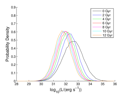
Refer to caption
Refer to caption
Figure 18: Evolution of the luminosity and period distributions with time for Model A1 which has L=ηEcutaγBbγE˙dγ𝐿𝜂superscriptsubscript𝐸cutsubscript𝑎𝛾superscript𝐵subscript𝑏𝛾superscript˙𝐸subscript𝑑𝛾L=\eta E_{\rm cut}^{a_{\gamma}}B^{b_{\gamma}}\dot{E}^{d_{\gamma}}. The legend gives the age of the MSPs in the corresponding distribution. These figures were made by selecting randomly from the highest likelihood parameter sets in our eight Markov chains for this model.

In Model A1, which has L=ηEcutaγBbγE˙dγ𝐿𝜂superscriptsubscript𝐸cutsubscript𝑎𝛾superscript𝐵subscript𝑏𝛾superscript˙𝐸subscript𝑑𝛾L=\eta E_{\rm cut}^{a_{\gamma}}B^{b_{\gamma}}\dot{E}^{d_{\gamma}}, relatively young members of the underlying population of MSPs are more likely to be resolved as they are brighter. This follows as E˙˙𝐸\dot{E}, and therefore luminosity, decreases with age. As the magnetic field strength is assumed constant for each MSP over time, it can be seen from Eqs. 2.18 and 2.17 that E˙P4proportional-to˙𝐸superscript𝑃4\dot{E}\propto P^{-4}. We show in Fig. 18 an example of how the log10(L)subscript10𝐿\log_{10}(L) and log10(P)subscript10𝑃\log_{10}(P) probability density functions evolve with age.

As can be seen from Fig. 4, the DTD peaks in the central 5.55.55.5 to 8.38.38.3 Gyr bin producing an age distribution that tends to plateau starting around 555 Gyr ago as shown in Fig. 7. As can be seen in Table 3 the posterior distributions of the parameters are similar for the GCE and No GCE cases. It can be seen in Table 2 that there is no significant difference in the WAIC for the DTD versus the uniform age distribution case. As can be seen in Fig. 7, for the case with the GCE, the fitted DTD produces an age distribution that is similar to the uniform case. For the uniform age distribution, the probability density is 0.10.10.1 for ages less than 101010 Gyr, and 00 elsewhere. The models that were significantly worse when the GCE was included remained significantly worse when it was not. The model for which the luminosity obeys L=ηEcutaγBbγE˙dγ𝐿𝜂superscriptsubscript𝐸cutsubscript𝑎𝛾superscript𝐵subscript𝑏𝛾superscript˙𝐸subscript𝑑𝛾L=\eta E_{\rm cut}^{a_{\gamma}}B^{b_{\gamma}}\dot{E}^{d_{\gamma}} remained the best model whether the GCE was included or not, i.e., models A1 and A2 were the best models when the GCE was included and Models B1 and B2 were the best models when the GCE was not included.

As can be seen from Fig. 13, there is a small difference in the GCE spectrum for the Model A1 and A2. This is due to the spectral dependence on E˙˙𝐸\dot{E} in Eqs. 2.28 and 2.29 and also the different star formation rates for the bulge and disk which are illustrated in Fig. 1. However, as can be seen in Fig. 13, the differences in the predicted spectrum are negligible in comparison to the model prediction uncertainties. As can be seen in the top right panel of Fig. 6 the boxy bulge MSPs do have a median luminosity function that is less bright than the disk MSPs. However, the 95% interval band encompasses zero which is the no difference case. This shows that with the current levels of uncertainty the differences in the properties of the bulge and disk MSPs is not significant.
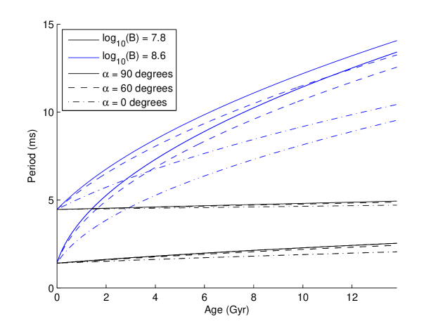
Refer to caption
Figure 19: Evolution of period with time for various magnetic field strengths B𝐵B, magnetic field axis angles α𝛼\alpha and initial periods PIsubscript𝑃𝐼P_{I}. The two PIsubscript𝑃𝐼P_{I} values used were 102.85superscript102.8510^{-2.85} s and 102.35superscript102.3510^{-2.35} s.

In Fig. 19 we show the evolution of period with time (Eq. 2.23) for MSPs with different properties. This indicates where the constraints on our models of the initial period and age distribution come from. For a resolved MSP with a weak magnetic field, the current period will be near the initial period even if the MSP is old, so these MSPs should be approximately distributed like the initial period distribution. This is a consequence of the fact that an MSP cannot be older than the universe. On the other hand, MSPs with strong magnetic fields will quickly, within a couple of Gyr, move out of the initial period distribution. This (relatively) rapid evolution of period means the distributions of PIsubscript𝑃𝐼P_{I} and α𝛼\alpha produce (for a given P𝑃P and B𝐵B) a range of possible ages for each MSP.

In Fig. 9 it is shown that, at 68% confidence level, for Model A1 between around 23000 and 54000 MSPs are needed in the bulge to produce the observed GCE. This is consistent with Gonthier et al. [18] in which they find, though with a different bulge density model and GCE spectrum, 34,200 MSPs are needed with 11,500 in the region of interest associated with the Gordon et al. [4] GCE spectrum. In Ploeg et al. [13] it was found that around (4.0±0.9)×104plus-or-minus4.00.9superscript104(4.0\pm 0.9)\times 10^{4} MSPs with L>1032 erg s1𝐿superscript1032superscript erg s1L>10^{32}\textrm{ erg s}^{-1} were needed to produce the GCE; here, as shown in Fig. 10, the required number is between about 13000 and 26000 at 95% confidence interval. Note the difference between these two estimates is not statistically significant; the slight discrepancy is likely due to the more accurate bulge geometric model, luminosity function, and GCE spectrum used in the current study.

In order to check the sensitivity of the results to the particular GCE spectrum used we also fitted Model A1 to alternative spectra. Using Bartels et al. [6], we found a small number of changes where the median of a parameter was outside the 68%percent6868\% ranges shown in Table 3. The ratio of nuclear bulge and boxy bulge MSPs is lower with log10(Nnb/Nbb)=0.90+0.060.06subscript10subscript𝑁nbsubscript𝑁bb0.900.060.06\log_{10}(N_{\rm nb}/N_{\rm bb})=-0.90\begin{subarray}{c}+0.06\\ -0.06\end{subarray}. The relationship between ΓΓ\Gamma and E˙˙𝐸\dot{E} is steeper with aΓ=0.52+0.070.08subscript𝑎Γ0.520.070.08a_{\Gamma}=0.52\begin{subarray}{c}+0.07\\ -0.08\end{subarray}. The fifth DTD bin is constrained strongly to be near 00 with DTD p(11.1 - 13.8 Gyr)=0.01+0.030.01DTD 𝑝11.1 - 13.8 Gyr0.010.030.01\textrm{DTD }p(11.1\textrm{ - }13.8\textrm{ Gyr})=0.01\begin{subarray}{c}+0.03\\ -0.01\end{subarray}. These changes are likely to be caused by the steep slope on both the low and high energy ends of the boxy bulge spectrum. For the spectrum in Calore et al. [40], we had no nuclear bulge, but otherwise the results were consistent with those using the spectra of Macias et al. [7].

It can be seen in Fig. 12 that we find a probability of 0.160.160.16 that no bulge MSPs would have been resolved at present, with a median of 222 resolved. With a doubling and quadrupling of detection sensitivity, respectively, a median of 101010 and 353535 would be expected to be resolved. In Table 8 we provide a list of resolved MSPs with a significant probability (greater than 5%percent55\%) of being bulge MSPs according to Model A1. These probabilities are worked out in Eq. B.3 by evaluating the contribution of the bulge to the corresponding MSP’s likelihood.

The probability of resolved MSP i𝑖i being a bulge MSP can be thought of as a draw from a single trial binomial distribution with probability p(Bulge MSPi)𝑝subscriptBulge MSP𝑖p(\textrm{Bulge MSP}_{i}) and therefore also having an expectation value of p(Bulge MSPi)𝑝subscriptBulge MSP𝑖p(\textrm{Bulge MSP}_{i}). Using the linearity of expectation, this implies that the expected number of resolved bulge MSPs in the current data is ip(Bulge MSPi)=1.1subscript𝑖𝑝subscriptBulge MSP𝑖1.1\sum_{i}p(\textrm{Bulge MSP}_{i})=1.1 where the sum is over all resolved MSPs including those listed in Table 8. This is at the lower end of, but consistent with, the range seen in Fig. 12 produced based on the fitted model parameters.

Note that there is also some systematic uncertainty in the distance to the MSPs which is hard to quantify. For example, in Table 4 of ref. [41] they have a distance of 3.4 kpc for J1747–4036 while we have a distance of 7.3+0.70.77.30.70.77.3\begin{subarray}{c}+0.7\\ -0.7\end{subarray} kpc. Also in Table 2.2 of ref. [42] they have a distance of 3.1 kpc for J1855–1436 while we have a distance of 5.3+0.60.65.30.60.65.3\begin{subarray}{c}+0.6\\ -0.6\end{subarray} kpc. These difference may be due to a change in model of the Galactic free electron density. According to the ATNF online database444https://www.atnf.csiro.au/research/pulsar/psrcat/ J1747–4036 and J1855–1436 have distances of 7.15 kpc and 5.13 kpc respectively which are compatible with our values. Also, in Table 2 of ref. [43] they have a dispersion measure distance of 1.8 kpc for J1811–2405 while we have a parallax derived distance of 5+11251125\begin{subarray}{c}+11\\ -2\end{subarray} kpc.

In Fig. 20 the locations of resolved MSPs are shown along with a simulated distribution of disk and bulge MSPs. The elongated nature of the bulge geometry does not play a big role in the probability of having a resolved bulge MSP. This can be seen by changing the boxy bulge geometry in Eq. 2.2 to a spherically symmetric geometry with ρboxybulger2.4proportional-tosubscript𝜌boxybulgesuperscript𝑟2.4\rho_{\rm boxy~{}bulge}\propto r^{-2.4} up to r=3.1𝑟3.1r=3.1 kpc and ρboxybulge=0subscript𝜌boxybulge0\rho_{\rm boxy~{}bulge}=0 for larger radii [13]. We then find that 2±2plus-or-minus222\pm 2 MSPs are expected to be resolved for Model A1. Also, for this spherically symmetric bulge case, the MSPs in Table 8 have probabilities of 0.5, 0.2, and 4×1044superscript1044\times 10^{-4} respectively. So only PSR J1855-1436, with its high l=20.4𝑙superscript20.4l=20.4^{\circ}, is significantly affected by the bulge geometry.

Name Bulge Probability l𝑙l (deg) b𝑏b (deg) d𝑑d (kpc) L𝐿L (×1034absentsuperscript1034\times 10^{34} erg s-1) d𝑑d percentile L𝐿L percentile
PSR J1747-4036 0.4 9.89.8-9.8 6.46.4-6.4 7.3+0.70.77.30.70.77.3\begin{subarray}{c}+0.7\\ -0.7\end{subarray} 7.7+1.81.57.71.81.57.7\begin{subarray}{c}+1.8\\ -1.5\end{subarray} 100100100 999999
PSR J1811-2405 0.5 7.17.17.1 2.52.5-2.5 5+11251125\begin{subarray}{c}+11\\ -2\end{subarray} 5+47454745\begin{subarray}{c}+47\\ -4\end{subarray} 969696 979797
PSR J1855-1436 0.1 20.420.420.4 7.67.6-7.6 5.3+0.60.65.30.60.65.3\begin{subarray}{c}+0.6\\ -0.6\end{subarray} 1.8+0.50.41.80.50.41.8\begin{subarray}{c}+0.5\\ -0.4\end{subarray} 989898 919191
Table 8: Details of MSPs with significant probability (greater than 5%percent55\%) of coming from bulge population for Model A1. The names are from the Public List of LAT-Detected Gamma-Ray Pulsarsfootnote 1. Distances are medians and 68%percent6868\% intervals found by sampling the parallax uncertainty distribution if available or otherwise using the dispersion measure and randomly sampling the parameters of the YMW16 electron density model. Luminosities are medians and 68%percent6868\% intervals found by additionally sampling from the flux uncertainty distribution. Percentiles are the fraction of resolved MSPs with smaller or equal luminosity/distance. This excludes MSPs without available distance estimates.
Refer to caption
Refer to caption
Figure 20: Simulated distribution of disk and bulge MSPs for Model A1 (L=ηEcutaγBbγE˙dγ𝐿𝜂superscriptsubscript𝐸cutsubscript𝑎𝛾superscript𝐵subscript𝑏𝛾superscript˙𝐸subscript𝑑𝛾L=\eta E_{\rm cut}^{a_{\gamma}}B^{b_{\gamma}}\dot{E}^{d_{\gamma}}). Also shown are those resolved MSPs with available distance estimates. These figures were made by selecting randomly from the highest likelihood parameter sets in our eight Markov chains for this model. Red circles are the MSPs in Table 8.

As shown in Fig. 11, the disk, nuclear bulge and boxy bulge have a consistent MSP to stellar mass ratio. This is a good confirmation of our assumption that the population of individual, resolved MSPs belonging mostly to the disk population, on the one hand, and the apparently diffuse γ𝛾\gamma-ray emission from the GCE, on the other, can be self-consistently explained as arising from MSPs drawn from the same underlying luminosity function given by Eq. 2.24.

5 Conclusion

We compared a wide variety of luminosity function models for the Fermi-LAT gamma-ray MSP data. We found a convincing preference for Model A1 for which L=ηEcutaγBbγE˙dγ𝐿𝜂superscriptsubscript𝐸cutsubscript𝑎𝛾superscript𝐵subscript𝑏𝛾superscript˙𝐸subscript𝑑𝛾L=\eta E_{\rm cut}^{a_{\gamma}}B^{b_{\gamma}}\dot{E}^{d_{\gamma}} with a significantly positive aγ=1.2±0.3subscript𝑎𝛾plus-or-minus1.20.3a_{\gamma}=1.2\pm 0.3 and dγ=0.5±0.1subscript𝑑𝛾plus-or-minus0.50.1d_{\gamma}=0.5\pm 0.1. Thus we confirm the result obtained by Kalapotharakos et al. [17] that MSP gamma-ray emission is consistent with curvature radiation and inconsistent with synchrotron radiation. By comparing with other models, we showed that the main source of the positive aγsubscript𝑎𝛾a_{\gamma} result was the need to account for a significant logarithmic correlation in the data between the Ecutsubscript𝐸cutE_{\rm cut} and distance in the form of the dispersion measure. We also showed that the main source of the positive dγsubscript𝑑𝛾d_{\gamma} was due to the significant logarithmic correlation in the data between the period and the distance in the form of the dispersion measure.

Additionally, we found that it was warranted to include a relationship between the spectral parameters and E˙˙𝐸\dot{E}. In particular we found that a linear relationship between the mean of the spectral index μΓsubscript𝜇Γ\mu_{\Gamma} and the log10(E˙)subscript10˙𝐸\log_{10}(\dot{E}), as specified in Eq. 2.29, had a significantly positive slope of aΓ=0.4±0.08subscript𝑎Γplus-or-minus0.40.08a_{\Gamma}=0.4\pm 0.08. We identified the source of this positive slope to be the need to explain the significant correlation between ΓΓ\Gamma and log10(P)subscript10𝑃\log_{\rm 10}(P) seen in the data.

We non-parametrically estimated the delay time distribution of the MSPs but found the current data does not strongly constrain it. Our results obtained using a DTD prescription are also not significantly different from those obtained assuming a uniform age distribution for the MSPs.

Our results demonstrate that the population of MSPs that can explain the gamma-ray signal from the resolved MSPs in the Galactic disk and the unresolved MSPs in the boxy bulge and nuclear bulge can consistently be described as arising from a common evolutionary trajectory for some subset of astrophysical sources common to all these different environments. We do not require that there is anything unusual about inner Galaxy MSPs to explain the GCE. We also found that the current data is not accurate enough to be sensitive to the small differences between the bulge and disk MSPs.

We estimated that there are between about 20 and 50 thousand MSPs in the boxy bulge at 68% confidence interval. We identified three candidate resolved MSPs (J1747-4036, J1811-2405, J1855-1436) that have significant probabilities (0.4, 0.5 and 0.1 respectively) of being members of the boxy bulge population. We estimate that this number would increase to 9 and 31 resolved boxy bulge MSPs were the point source sensitivity of the gamma-ray observations doubled or quadrupled, respectively.

References

  • [1] L. Goodenough and D. Hooper, Possible Evidence For Dark Matter Annihilation In The Inner Milky Way From The Fermi Gamma Ray Space Telescope, arXiv e-prints (2009) arXiv:0910.2998 [0910.2998].
  • [2] D. Hooper and T. Linden, Origin of the gamma rays from the galactic center, Physical Review D 84 (2011) .
  • [3] K.N. Abazajian and M. Kaplinghat, Detection of a Gamma-Ray Source in the Galactic Center Consistent with Extended Emission from Dark Matter Annihilation and Concentrated Astrophysical Emission, Phys. Rev. D86 (2012) 083511 [1207.6047].
  • [4] C. Gordon and O. Macias, Dark Matter and Pulsar Model Constraints from Galactic Center Fermi-LAT Gamma Ray Observations, Phys. Rev. D88 (2013) 083521 [1306.5725].
  • [5] O. Macias, C. Gordon, R.M. Crocker, B. Coleman, D. Paterson, S. Horiuchi et al., Galactic bulge preferred over dark matter for the galactic centre gamma-ray excess, Nature Astronomy 2 (2018) 387–392.
  • [6] R. Bartels, E. Storm, C. Weniger and F. Calore, The Fermi-LAT GeV excess as a tracer of stellar mass in the Galactic bulge, Nature Astronomy (2018) [1711.04778].
  • [7] O. Macias, S. Horiuchi, M. Kaplinghat, C. Gordon, R.M. Crocker and D.M. Nataf, Strong evidence that the galactic bulge is shining in gamma rays, JCAP 2019 (2019) 042 [1901.03822].
  • [8] K.N. Abazajian, S. Horiuchi, M. Kaplinghat, R.E. Keeley and O. Macias, Strong constraints on thermal relic dark matter from Fermi-LAT observations of the Galactic Center, Phys. Rev. D 102 (2020) 043012 [2003.10416].
  • [9] B. Coleman, D. Paterson, C. Gordon, O. Macias and H. Ploeg, Maximum entropy estimation of the Galactic bulge morphology via the VVV Red Clump, MNRAS 495 (2020) 3350 [1911.04714].
  • [10] K.N. Abazajian, The Consistency of Fermi-LAT Observations of the Galactic Center with a Millisecond Pulsar Population in the Central Stellar Cluster, JCAP 1103 (2011) 010 [1011.4275].
  • [11] D. Hooper and G. Mohlabeng, The Gamma-Ray Luminosity Function of Millisecond Pulsars and Implications for the GeV Excess, JCAP 1603 (2016) 049 [1512.04966].
  • [12] D. Haggard, C. Heinke, D. Hooper and T. Linden, Low mass x-ray binaries in the inner galaxy: implications for millisecond pulsars and the gev excess, Journal of Cosmology and Astroparticle Physics 2017 (2017) 056–056.
  • [13] H. Ploeg, C. Gordon, R. Crocker and O. Macias, Consistency Between the Luminosity Function of Resolved Millisecond Pulsars and the Galactic Center Excess, JCAP 1708 (2017) 015 [1705.00806].
  • [14] R.T. Bartels, T.D.P. Edwards and C. Weniger, Bayesian model comparison and analysis of the Galactic disc population of gamma-ray millisecond pulsars, MNRAS 481 (2018) 3966 [1805.11097].
  • [15] R.M. Crocker et al., Diffuse Galactic antimatter from faint thermonuclear supernovae in old stellar populations, 1607.03495.
  • [16] Fermi-LAT collaboration, The Second Fermi Large Area Telescope Catalog of Gamma-ray Pulsars, Astrophys. J. Suppl. 208 (2013) 17 [1305.4385].
  • [17] C. Kalapotharakos, A.K. Harding, D. Kazanas and Z. Wadiasingh, A fundamental plane for gamma-ray pulsars, The Astrophysical Journal 883 (2019) L4.
  • [18] P.L. Gonthier, A.K. Harding, E.C. Ferrara, S.E. Frederick, V.E. Mohr and Y.-M. Koh, Population Syntheses of Millisecond Pulsars from the Galactic Disk and Bulge, ApJ 863 (2018) 199 [1806.11215].
  • [19] Fermi-LAT collaboration, Fermi Large Area Telescope Fourth Source Catalog Data Release 2, 2005.11208.
  • [20] R.N. Manchester, G.B. Hobbs, A. Teoh and M. Hobbs, The Australia Telescope National Facility pulsar catalogue, Astron. J. 129 (2005) 1993 [astro-ph/0412641].
  • [21] H.T. Freudenreich, Cobe’s galactic bar and disk, Astrophys. J. 492 (1998) 495 [astro-ph/9707340].
  • [22] J.M. Yao, R.N. Manchester and N. Wang, A New Electron-density Model for Estimation of Pulsar and FRB Distances, ApJ 835 (2017) 29 [1610.09448].
  • [23] S. Weinberg, Cosmology, Oxford University Press (2008).
  • [24] P.A.R. Ade, N. Aghanim, C. Armitage-Caplan, M. Arnaud, M. Ashdown, F. Atrio-Barandela et al., Planck2013 results. xvi. cosmological parameters, Astronomy & Astrophysics 571 (2014) A16.
  • [25] F. Nogueras-Lara, R. Schödel, A.T. Gallego-Calvente, E. Gallego-Cano, B. Shahzamanian, H. Dong et al., Early formation and recent starburst activity in the nuclear disk of the Milky Way, Nature Astronomy 4 (2019) 377 [1910.06968].
  • [26] R.G. Carlberg and K.A. Innanen, Galactic Chaos and the Circular Velocity at the Sun, Astronom. J. 94 (1987) 666.
  • [27] K. Kuijken and G. Gilmore, The mass distribution in the galactic disc. I - A technique to determine the integral surface mass density of the disc near the sun., MNRAS 239 (1989) 571.
  • [28] R. Schönrich, J. Binney and W. Dehnen, Local kinematics and the local standard of rest, MNRAS 403 (2010) 1829 [0912.3693].
  • [29] A. Spitkovsky, Time-dependent Force-free Pulsar Magnetospheres: Axisymmetric and Oblique Rotators, ApJ 648 (2006) L51 [astro-ph/0603147].
  • [30] H. Haario, E. Saksman and J. Tamminen, An adaptive metropolis algorithm, Bernoulli 7 (2001) 223.
  • [31] W. Cash, Parameter estimation in astronomy through application of the likelihood ratio., ApJ 228 (1979) 939.
  • [32] A.C. Cameron and P.K. Trivedi, Regression Analysis of Count Data,, Cambridge University Press (1998).
  • [33] A. Gelman, J.B. Carlin, H.S. Stern, D.B. Dunson, A. Vehtari and D.B. Rubin, Bayesian Data Analysis, CRC Press, 3 ed. (2013).
  • [34] S. Watanabe, Asymptotic Equivalence of Bayes Cross Validation and Widely Applicable Information Criterion in Singular Learning Theory, arXiv e-prints (2010) arXiv:1004.2316 [1004.2316].
  • [35] S. Wilks, The Large-Sample Distribution of the Likelihood Ratio for Testing Composite Hypotheses, Annals Math. Statist. 9 (1938) 60.
  • [36] D. Foreman-Mackey, corner.py: Scatterplot matrices in python, The Journal of Open Source Software 1 (2016) 24.
  • [37] A. Gelman, Two simple examples for understanding posterior p-values whose distributions are far from uniform, Electronic Journal of Statistics 7 (2013) 2995.
  • [38] J. Bland-Hawthorn and O. Gerhard, The Galaxy in Context: Structural, Kinematic, and Integrated Properties, Annual Review of Astronomy and Astrophysics 54 (2016) 529 [1602.07702].
  • [39] M. Betancourt, Cruising the simplex: Hamiltonian Monte Carlo and the Dirichlet distribution, in American Institute of Physics Conference Series, P. Goyal, A. Giffin, K.H. Knuth and E. Vrscay, eds., vol. 1443 of American Institute of Physics Conference Series, pp. 157–164, May, 2012, DOI [1010.3436].
  • [40] F. Calore, I. Cholis and C. Weniger, Background Model Systematics for the Fermi GeV Excess, JCAP 1503 (2015) 038 [1409.0042].
  • [41] F. Camilo, M. Kerr, P.S. Ray, S.M. Ransom, J. Sarkissian, H.T. Cromartie et al., Parkes Radio Searches of Fermi Gamma-Ray Sources and Millisecond Pulsar Discoveries, ApJ 810 (2015) 85 [1507.04451].
  • [42] S. Sanpa-arsa, Searching for new millisecond pulsars with the GBT in Fermi unassociated sources, Ph.D. thesis, University of Virginia, 7, 2016.
  • [43] C. Ng, L. Guillemot, P.C.C. Freire, M. Kramer, D.J. Champion, I. Cognard et al., A Shapiro delay detection in the pulsar binary system PSR J1811-2405, MNRAS 493 (2020) 1261 [2002.01009].

Acknowledgments

HP is supported by a University of Canterbury Doctoral Scholarship. RMC acknowledges an Australian Research Council Discovery award (DP190101258). O.M. acknowledges support by JSPS KAKENHI Grant Numbers JP17H04836, JP18H04340, JP18H04578, and JP20K14463. This work was supported by World Premier International Research Center Initiative (WPI Initiative), MEXT, Japan.

Appendix A Likelihood probability density function of resolved MSPs

In this appendix we implicitly assume that all probabilities are conditioned on the parameters (𝜽𝜽\boldsymbol{\theta}). Also, as all of our expression here are also for an individual MSP we leave the subscript on each observational quantity as implicit. As an example of these conventions, p(obs|l,b,F)𝑝conditionalobs𝑙𝑏𝐹p({\rm obs}|l,b,F) is equivalent to p(obs|li,bi,Fi,𝜽)𝑝conditionalobssubscript𝑙𝑖subscript𝑏𝑖subscript𝐹𝑖𝜽p({\rm obs}|l_{i},b_{i},F_{i},\boldsymbol{\theta}).

We assume the likelihood of observed MSPs with/without a parallax distance measurement depends only on distance d𝑑d:

p(obs,l,b,d,P,P˙,μl,μb,F,Ecut,Γ,parallax/not parallax)=p(obs,l,b,d,P,P˙,μl,μb,F,Ecut,Γ)×p(parallax/not parallax|d)𝑝obs𝑙𝑏𝑑𝑃˙𝑃subscript𝜇𝑙subscript𝜇𝑏𝐹subscript𝐸cutΓparallax/not parallax𝑝obs𝑙𝑏𝑑𝑃˙𝑃subscript𝜇𝑙subscript𝜇𝑏𝐹subscript𝐸cutΓ𝑝conditionalparallax/not parallax𝑑\begin{multlined}p({\rm obs},l,b,d,P,\dot{P},\mu_{l},\mu_{b},F,E_{\rm cut},\Gamma,\textrm{parallax/not parallax})=p({\rm obs},l,b,d,P,\dot{P},\mu_{l},\mu_{b},F,E_{\rm cut},\Gamma)\\ \times p(\textrm{parallax/not parallax}|d)\end{multlined}p({\rm obs},l,b,d,P,\dot{P},\mu_{l},\mu_{b},F,E_{\rm cut},\Gamma,\textrm{parallax/not parallax})=p({\rm obs},l,b,d,P,\dot{P},\mu_{l},\mu_{b},F,E_{\rm cut},\Gamma)\\ \times p(\textrm{parallax/not parallax}|d) (A.1)

where the probability of a parallax measurement given distance d𝑑d is given by Eq. 2.45. In terms of the various components of the MSP model, the probability density function of resolved MSPs at l𝑙l, b𝑏b, d𝑑d, P𝑃P, P˙˙𝑃\dot{P}, μlsubscript𝜇𝑙\mu_{l}, μbsubscript𝜇𝑏\mu_{b}, F𝐹F, Ecutsubscript𝐸cutE_{\rm cut} and ΓΓ\Gamma is:

p(obs,l,b,d,P,P˙,μl,μb,F,Ecut,Γ)=p(obs,l,b,d,P,P˙,μl,μb,F,Ecut,Γ,α,PI)dαdPI𝑝obs𝑙𝑏𝑑𝑃˙𝑃subscript𝜇𝑙subscript𝜇𝑏𝐹subscript𝐸cutΓ𝑝obs𝑙𝑏𝑑𝑃˙𝑃subscript𝜇𝑙subscript𝜇𝑏𝐹subscript𝐸cutΓ𝛼subscript𝑃𝐼𝛼subscript𝑃𝐼p({\rm obs},l,b,d,P,\dot{P},\mu_{l},\mu_{b},F,E_{\rm cut},\Gamma)=\int\int p({\rm obs},l,b,d,P,\dot{P},\mu_{l},\mu_{b},F,E_{\rm cut},\Gamma,\alpha,P_{I})\,\differential\alpha\,\differential P_{I} (A.2)

where we have integrated over the unknown magnetic axis angle and initial period. Then:

p(obs,l,b,d,P,P˙,μl,μb,F,Ecut,Γ,α,PI)=p(obs|l,b,F)p(F|l,b,d,P,P˙,μl,μb,Ecut,α)×p(Ecut,Γ|l,b,d,P,P˙,μl,μb)p(P,P˙|l,b,d,μl,μb,α,PI)p(μl,μb|l,b,d)×p(l,b,d)p(α)p(PI)𝑝obs𝑙𝑏𝑑𝑃˙𝑃subscript𝜇𝑙subscript𝜇𝑏𝐹subscript𝐸cutΓ𝛼subscript𝑃𝐼𝑝conditionalobs𝑙𝑏𝐹𝑝conditional𝐹𝑙𝑏𝑑𝑃˙𝑃subscript𝜇𝑙subscript𝜇𝑏subscript𝐸cut𝛼𝑝subscript𝐸cutconditionalΓ𝑙𝑏𝑑𝑃˙𝑃subscript𝜇𝑙subscript𝜇𝑏𝑝𝑃conditional˙𝑃𝑙𝑏𝑑subscript𝜇𝑙subscript𝜇𝑏𝛼subscript𝑃𝐼𝑝subscript𝜇𝑙conditionalsubscript𝜇𝑏𝑙𝑏𝑑𝑝𝑙𝑏𝑑𝑝𝛼𝑝subscript𝑃𝐼\begin{multlined}p({\rm obs},l,b,d,P,\dot{P},\mu_{l},\mu_{b},F,E_{\rm cut},\Gamma,\alpha,P_{I})=p({\rm obs}|l,b,F)p(F|l,b,d,P,\dot{P},\mu_{l},\mu_{b},E_{\rm cut},\alpha)\\ \times p(E_{\rm cut},\Gamma|l,b,d,P,\dot{P},\mu_{l},\mu_{b})p(P,\dot{P}|l,b,d,\mu_{l},\mu_{b},\alpha,P_{I})p(\mu_{l},\mu_{b}|l,b,d)\\ \times p(l,b,d)p(\alpha)p(P_{I})\end{multlined}p({\rm obs},l,b,d,P,\dot{P},\mu_{l},\mu_{b},F,E_{\rm cut},\Gamma,\alpha,P_{I})=p({\rm obs}|l,b,F)p(F|l,b,d,P,\dot{P},\mu_{l},\mu_{b},E_{\rm cut},\alpha)\\ \times p(E_{\rm cut},\Gamma|l,b,d,P,\dot{P},\mu_{l},\mu_{b})p(P,\dot{P}|l,b,d,\mu_{l},\mu_{b},\alpha,P_{I})p(\mu_{l},\mu_{b}|l,b,d)\\ \times p(l,b,d)p(\alpha)p(P_{I}) (A.3)

The probability of observing an MSP with flux F𝐹F at l𝑙l and b𝑏b is given by Eq. 2.34, so:

p(obs|l,b,F)=p(FthF|l,b)𝑝conditionalobs𝑙𝑏𝐹𝑝subscript𝐹thconditional𝐹𝑙𝑏p({\rm obs}|l,b,F)=p(F_{\rm th}\leq F|l,b) (A.4)

Some of the data used is given in the form of 𝒚jsubscript𝒚𝑗\boldsymbol{y}_{j} where 𝒚𝒚\boldsymbol{y} is not one of the directly modeled MSP parameters. In this case we perform a transformation to the observed parameter:

p(,𝒚j,)=d𝒚p(𝒚j|𝒚)|𝑱|p(,𝒙(𝒚),)𝑝subscript𝒚𝑗𝒚𝑝conditionalsubscript𝒚𝑗𝒚𝑱𝑝𝒙𝒚p(...,\boldsymbol{y}_{j},...)=\int\differential\boldsymbol{y}p(\boldsymbol{y}_{j}|\boldsymbol{y})\lvert\boldsymbol{J}\rvert p(...,\boldsymbol{x}(\boldsymbol{y}),...) (A.5)

where |𝑱|𝑱\lvert\boldsymbol{J}\rvert is the Jacobian determinant of the transformation from 𝒚𝒚\boldsymbol{y} to 𝒙𝒙\boldsymbol{x}, so 𝑱i,j=xi(𝒚)/yjsubscript𝑱𝑖𝑗subscript𝑥𝑖𝒚subscript𝑦𝑗\boldsymbol{J}_{i,j}=\partial x_{i}(\boldsymbol{y})/\partial y_{j}. This transformation is needed for integrating over uncertainty in distance where we have either parallax (ω𝜔\omega), where ω=1/d𝜔1𝑑\omega=1/d, or dispersion measure (DM), where DM=0dne(s)dsDMsuperscriptsubscript0𝑑subscript𝑛𝑒𝑠𝑠\textrm{DM}=\int_{0}^{d}n_{e}(s)\differential s with ne(s)subscript𝑛𝑒𝑠n_{e}(s) being the free electron density at distance s𝑠s.

The probability density function of an MSP having flux F𝐹F conditional upon it’s other parameters is, given log(F)=log(η)+f()𝐹𝜂𝑓\log(F)=\log(\eta)+f(...) where f()𝑓f(...) is some function which doesn’t depend on η𝜂\eta:

p(F|l,b,d,P,P˙,μl,μb,Ecut,α)=p(η|l,b,d,P,P˙,μl,μb,Ecut,α)ηF=p(η|l,b,d,P,P˙,μl,μb,Ecut,α)ηF𝑝conditional𝐹𝑙𝑏𝑑𝑃˙𝑃subscript𝜇𝑙subscript𝜇𝑏subscript𝐸cut𝛼𝑝conditional𝜂𝑙𝑏𝑑𝑃˙𝑃subscript𝜇𝑙subscript𝜇𝑏subscript𝐸cut𝛼𝜂𝐹𝑝conditional𝜂𝑙𝑏𝑑𝑃˙𝑃subscript𝜇𝑙subscript𝜇𝑏subscript𝐸cut𝛼𝜂𝐹\begin{split}p(F|l,b,d,P,\dot{P},\mu_{l},\mu_{b},E_{\rm cut},\alpha)&=p(\eta|l,b,d,P,\dot{P},\mu_{l},\mu_{b},E_{\rm cut},\alpha)\frac{\partial\eta}{\partial F}\\ &=p(\eta|l,b,d,P,\dot{P},\mu_{l},\mu_{b},E_{\rm cut},\alpha)\frac{\eta}{F}\end{split} (A.6)

After a change of variables from period P𝑃P and observed period derivative P˙˙𝑃\dot{P} to magnetic field strength B𝐵B and age t𝑡t, we get:

p(P,P˙|l,b,d,μl,μb,α,PI)=p(B,t|l,b,d,α,PI)|BPtP˙BP˙tP|𝑝𝑃conditional˙𝑃𝑙𝑏𝑑subscript𝜇𝑙subscript𝜇𝑏𝛼subscript𝑃𝐼𝑝𝐵conditional𝑡𝑙𝑏𝑑𝛼subscript𝑃𝐼𝐵𝑃𝑡˙𝑃𝐵˙𝑃𝑡𝑃p(P,\dot{P}|l,b,d,\mu_{l},\mu_{b},\alpha,P_{I})=p(B,t|l,b,d,\alpha,P_{I})\left\lvert\frac{\partial B}{\partial P}\frac{\partial t}{\partial\dot{P}}-\frac{\partial B}{\partial\dot{P}}\frac{\partial t}{\partial P}\right\rvert (A.7)

where to evaluate the Jacobian in the above equation we rewrite Eq. 2.21 as

P˙Shklovskii=C1Psubscript˙𝑃Shklovskiisubscript𝐶1𝑃\dot{P}_{\rm Shklovskii}=C_{1}P (A.8)

where C1subscript𝐶1C_{1} is a term that is independent of P𝑃P and P˙˙𝑃\dot{P}. We also rewrite Eq. 2.22 as

P˙Galactic=C2Psubscript˙𝑃Galacticsubscript𝐶2𝑃\dot{P}_{\rm Galactic}=C_{2}P (A.9)

where C2subscript𝐶2C_{2} is also independent of P𝑃P and P˙˙𝑃\dot{P}. We then obtain an equation for B𝐵B in terms of P𝑃P and P˙˙𝑃\dot{P} using the above two equations with Eqs. 2.20 and 2.18 to get

B2=c3IP(P(C1+C2)+P˙)π2R6(sin2(α)+1)superscript𝐵2superscript𝑐3𝐼𝑃𝑃subscript𝐶1subscript𝐶2˙𝑃superscript𝜋2superscript𝑅6superscript2𝛼1B^{2}=\frac{c^{3}IP\left(-P({C}_{1}+{C}_{2})+\dot{P}\right)}{\pi^{2}R^{6}\left(\sin^{2}(\alpha)+1\right)} (A.10)

Next we obtain an equation for t𝑡t in terms of P𝑃P and P˙˙𝑃\dot{P} by substituting the above equation into Eq. 2.23 and solving t𝑡t to get

t=PI2P22P((C1+C2)PP˙)𝑡superscriptsubscript𝑃𝐼2superscript𝑃22𝑃subscript𝐶1subscript𝐶2𝑃˙𝑃t=\frac{P_{I}^{2}-P^{2}}{2P\left(\left(C_{1}+{C}_{2}\right)P-\dot{P}\right)} (A.11)

Using the above two equations we can then solve for the Jacobian term in Eq. A.7 to get

|BPtP˙BP˙tP|=c6I2P22π4R12(1+sin2(α))2B3𝐵𝑃𝑡˙𝑃𝐵˙𝑃𝑡𝑃superscript𝑐6superscript𝐼2superscript𝑃22superscript𝜋4superscript𝑅12superscript1superscript2𝛼2superscript𝐵3\left\lvert\frac{\partial B}{\partial P}\frac{\partial t}{\partial\dot{P}}-\frac{\partial B}{\partial\dot{P}}\frac{\partial t}{\partial P}\right\rvert=\frac{c^{6}I^{2}P^{2}}{2\pi^{4}R^{12}(1+\sin^{2}(\alpha))^{2}B^{3}} (A.12)

where we have used Eq. A.10 to eliminate C1subscript𝐶1C_{1} and C2subscript𝐶2C_{2}. Similarly, using Eq. 2.11, v/μdproportional-to𝑣𝜇𝑑\partial v/\partial\mu\propto d, so we find for proper motion:

p(μl,μb|l,b,d)p(vl,vb|l,b,d)d2proportional-to𝑝subscript𝜇𝑙conditionalsubscript𝜇𝑏𝑙𝑏𝑑𝑝subscript𝑣𝑙conditionalsubscript𝑣𝑏𝑙𝑏𝑑superscript𝑑2p(\mu_{l},\mu_{b}|l,b,d)\propto p(v_{l},v_{b}|l,b,d)d^{2} (A.13)

where the proportionality constant is independent of our parameters and data and so does not affect our results. For position:

p(l,b,d)p(x,y,z)d2cos(b)proportional-to𝑝𝑙𝑏𝑑𝑝𝑥𝑦𝑧superscript𝑑2𝑏p(l,b,d)\propto p(x,y,z)d^{2}\cos(b) (A.14)

where d2cos(b)superscript𝑑2𝑏d^{2}\cos(b) is proportional to the Jacobian of the change of variables from x𝑥x, y𝑦y and z𝑧z to l𝑙l, b𝑏b and d𝑑d:

x=R0+dcos(l)cos(b)y=dsin(l)cos(b)z=dsin(b)𝑥subscript𝑅0𝑑𝑙𝑏𝑦𝑑𝑙𝑏𝑧𝑑𝑏\begin{split}x&=-R_{0}+d\cos(l)\cos(b)\\ y&=d\sin(l)\cos(b)\\ z&=d\sin(b)\\ \end{split} (A.15)

The density of resolved MSPs is the sum of the density in the disk, boxy bulge and nuclear bulge populations:

ρ(obs,)=Ndiskpdisk(obs,)+Nbbpbb(obs,)+Nnbpnb(obs,)𝜌obssubscript𝑁disksubscript𝑝diskobssubscript𝑁bbsubscript𝑝bbobssubscript𝑁nbsubscript𝑝nbobs\rho(\textrm{obs},...)=N_{\rm disk}p_{\rm disk}(\textrm{obs},...)+N_{\rm bb}p_{\rm bb}(\textrm{obs},...)+N_{\rm nb}p_{\rm nb}(\textrm{obs},...) (A.16)

where we can calculate the number in each population using the parameters λressubscript𝜆res\lambda_{\rm res}, log10(Ndisk/Nbulge)subscript10subscript𝑁disksubscript𝑁bulge\log_{10}(N_{\rm disk}/N_{\rm bulge}) and log10(Nnb/Nbb)subscript10subscript𝑁nbsubscript𝑁bb\log_{10}(N_{\rm nb}/N_{\rm bb}) and solving with:

λres=Ndiskpdisk(obs)+Nbbpbb(obs)+Nnbpnb(obs)subscript𝜆ressubscript𝑁disksubscript𝑝diskobssubscript𝑁bbsubscript𝑝bbobssubscript𝑁nbsubscript𝑝nbobs\lambda_{\rm res}=N_{\rm disk}p_{\rm disk}(\textrm{obs})+N_{\rm bb}p_{\rm bb}(\textrm{obs})+N_{\rm nb}p_{\rm nb}(\textrm{obs}) (A.17)

where each p(obs)𝑝obsp({\rm obs}) is evaluated using Eq. 2.41 for the corresponding spatial distribution.

In evaluating the likelihood for a given set of parameters, we used importance sampling to estimate integrals. As an example, in the case of the integrals over PIsubscript𝑃𝐼P_{I} and α𝛼\alpha in Eq. A.2 this integral becomes:

p(obs,l,b,d,P,P˙,μl,μb,F,Ecut,Γ)=p(obs,l,b,d,P,P˙,μl,μb,F,Ecut,Γ,α,PI)dαdPI=p(obs,l,b,d,P,P˙,μl,μb,F,Ecut,Γ|α,PI)p(α)p(PI)dαdPI1Ni=1Np(obs,l,b,d,P,P˙,μl,μb,F,Ecut,Γ|αi,PIi)𝑝obs𝑙𝑏𝑑𝑃˙𝑃subscript𝜇𝑙subscript𝜇𝑏𝐹subscript𝐸cutΓ𝑝obs𝑙𝑏𝑑𝑃˙𝑃subscript𝜇𝑙subscript𝜇𝑏𝐹subscript𝐸cutΓ𝛼subscript𝑃𝐼𝛼subscript𝑃𝐼𝑝obs𝑙𝑏𝑑𝑃˙𝑃subscript𝜇𝑙subscript𝜇𝑏𝐹subscript𝐸cutconditionalΓ𝛼subscript𝑃𝐼𝑝𝛼𝑝subscript𝑃𝐼𝛼subscript𝑃𝐼1𝑁superscriptsubscript𝑖1𝑁𝑝obs𝑙𝑏𝑑𝑃˙𝑃subscript𝜇𝑙subscript𝜇𝑏𝐹subscript𝐸cutconditionalΓsubscript𝛼𝑖subscript𝑃𝐼𝑖\begin{split}p({\rm obs},l,b,d,P,\dot{P},\mu_{l},\mu_{b},F,E_{\rm cut},\Gamma)&=\int\int p({\rm obs},l,b,d,P,\dot{P},\mu_{l},\mu_{b},F,E_{\rm cut},\Gamma,\alpha,P_{I})\,\differential\alpha\,\differential P_{I}\\ &=\int\int p({\rm obs},l,b,d,P,\dot{P},\mu_{l},\mu_{b},F,E_{\rm cut},\Gamma|\alpha,P_{I})p(\alpha)p(P_{I})\,\differential\alpha\,\differential P_{I}\\ &\approx\frac{1}{N}\sum_{i=1}^{N}p({\rm obs},l,b,d,P,\dot{P},\mu_{l},\mu_{b},F,E_{\rm cut},\Gamma|\alpha_{i},P_{Ii})\end{split} (A.18)

where we sum over N𝑁N samples αisubscript𝛼𝑖\alpha_{i} and PIisubscript𝑃𝐼𝑖P_{Ii} from the probability distributions p(α)𝑝𝛼p(\alpha) and p(PI)𝑝subscript𝑃𝐼p(P_{I}).

Appendix B Measurement Uncertainties

For the measurements of F𝐹F, Ecutsubscript𝐸cutE_{\rm cut} and ΓΓ\Gamma we use the 4FGL covariance matrices555Kindly provided to us by Dr Jean Ballet of the Fermi-LAT collaboration. for the uncertainty in N0subscript𝑁0N_{0}, γ1subscript𝛾1\gamma_{1} and a𝑎a, with the spectrum of the form666”PLSuperExpCutoff2” at https://fermi.gsfc.nasa.gov/ssc/data/analysis/scitools/source_models.html:

dNdE=N0(EE0)γ1exp(aEγ2)𝑁𝐸subscript𝑁0superscript𝐸subscript𝐸0subscript𝛾1𝑎superscript𝐸subscript𝛾2\frac{\differential N}{\differential E}=N_{0}\left(\frac{E}{E_{0}}\right)^{\gamma_{1}}\exp(-aE^{\gamma_{2}}) (B.1)

where E0subscript𝐸0E_{0} and γ2=2/3subscript𝛾223\gamma_{2}=2/3 are fixed for each MSP.

For the small number of MSPs in 4FGL-DR2 that were not fitted with spectra in the form of Eq. B.1, we simply use the reported flux and its error, treating Ecutsubscript𝐸cutE_{\rm cut} and ΓΓ\Gamma as missing. Since the catalog required Γ>0Γ0\Gamma>0, we also treat Ecutsubscript𝐸cutE_{\rm cut} and ΓΓ\Gamma as missing in the case where some MSPs had ΓΓ\Gamma fixed near 00. If, based on central estimates of P˙˙𝑃\dot{P}, μ𝜇\mu and d𝑑d, P˙intsubscript˙𝑃int\dot{P}_{\rm int} appears to be negative for a particular MSP (i.e., the MSP is apparently spinning up) we treat P˙˙𝑃\dot{P} as missing. An apparently negative intrinsic period derivatives can result in the case that the true proper motion and/or distance is lower than the value we use, therefore causing the Shklovskii effect to be overestimated. An example of an updated proper motion measurement fixing this issue is given for PSR J1231-1411 in Abdo et al. [16]. A second potential cause of negative period derivative is radial acceleration in the direction of the sun significantly in excess of that accounted for by the P˙Galacticsubscript˙𝑃Galactic\dot{P}_{\rm Galactic} term in equations 2.20 and 2.22.

In the case of distance uncertainties, for the dispersion measure we use a method similar to that of Bartels et al. [14]: The relative uncertainty in the dispersion measure is typically very small, so we assume that it is measured exactly. The main source of distance uncertainty is, therefore, associated with the model of the free electron density along the line of sight for each MSP. We use the YMW16 model of Yao et al. [22] and integrate over the uncertainty in the model parameters θYMW16subscript𝜃YMW16\theta_{\rm YMW16} so that:

p(,DMj,)=dθYMW16p(θYMW16)p(,DMj,|θYMW16)=dθYMW16p(θYMW16)×|DMd(DMj,θYMW16)|p(,d(DMj,θYMW16),)=dθYMW16p(θYMW16)ne(d(DMj,θYMW16),θYMW16)p(,d(DMj,θYMW16),)𝑝subscriptDM𝑗subscript𝜃YMW16𝑝subscript𝜃YMW16𝑝subscriptDM𝑗conditionalsubscript𝜃YMW16subscript𝜃YMW16𝑝subscript𝜃YMW16DM𝑑subscriptDM𝑗subscript𝜃YMW16𝑝𝑑subscriptDM𝑗subscript𝜃YMW16subscript𝜃YMW16𝑝subscript𝜃YMW16subscript𝑛𝑒𝑑subscriptDM𝑗subscript𝜃YMW16subscript𝜃YMW16𝑝𝑑subscriptDM𝑗subscript𝜃YMW16\begin{split}p(...,\textrm{DM}_{j},...)&=\int\differential\theta_{\rm YMW16}p(\theta_{\rm YMW16})p(...,\textrm{DM}_{j},...|\theta_{\rm YMW16})\\ &=\!\begin{multlined}\int\differential\theta_{\rm YMW16}p(\theta_{\rm YMW16})\\ \times\left\lvert\frac{\partial}{\partial\textrm{DM}}d(\textrm{DM}_{j},\theta_{\rm YMW16})\right\rvert p(...,d(\textrm{DM}_{j},\theta_{\rm YMW16}),...)\end{multlined}\int\differential\theta_{\rm YMW16}p(\theta_{\rm YMW16})\\ \times\left\lvert\frac{\partial}{\partial\textrm{DM}}d(\textrm{DM}_{j},\theta_{\rm YMW16})\right\rvert p(...,d(\textrm{DM}_{j},\theta_{\rm YMW16}),...)\\ &=\int\differential\theta_{\rm YMW16}\frac{p(\theta_{\rm YMW16})}{n_{e}(d(\textrm{DM}_{j},\theta_{\rm YMW16}),\theta_{\rm YMW16})}p(...,d(\textrm{DM}_{j},\theta_{\rm YMW16}),...)\end{split} (B.2)

From Eqs. 2.43, 2.46 and A.16 we can work out the fraction of the likelihood contributed by the boxy bulge and nuclear bulge components for resolved MSP i𝑖i given the model parameters and data uncertainties:

p(Bulge MSPi)=ρbb(𝑫i)+ρnb(𝑫i)ρ(𝑫i)𝑝subscriptBulge MSP𝑖subscript𝜌bbsubscript𝑫𝑖subscript𝜌nbsubscript𝑫𝑖𝜌subscript𝑫𝑖p(\textrm{Bulge MSP}_{i})=\frac{\rho_{\rm bb}(\boldsymbol{D}_{i})+\rho_{\rm nb}(\boldsymbol{D}_{i})}{\rho(\boldsymbol{D}_{i})} (B.3)

where ρbb(𝑫i)=Nbbpbb(obs,𝑫i)subscript𝜌bbsubscript𝑫𝑖subscript𝑁bbsubscript𝑝bbobssubscript𝑫𝑖\rho_{\rm bb}(\boldsymbol{D}_{i})=N_{\rm bb}p_{\rm bb}(\textrm{obs},\boldsymbol{D}_{i}) and ρnb(𝑫i)=Nnbpnb(obs,𝑫i)subscript𝜌nbsubscript𝑫𝑖subscript𝑁nbsubscript𝑝nbobssubscript𝑫𝑖\rho_{\rm nb}(\boldsymbol{D}_{i})=N_{\rm nb}p_{\rm nb}(\textrm{obs},\boldsymbol{D}_{i}).

Appendix C Sampling methods

The disk model, given in Eq. 2.1, can be sampled from by sampling in cylindrical coordinates a random R𝑅R, z𝑧z and ϕitalic-ϕ\phi. The radial coordinate R𝑅R is drawn from:

p(R)=1σr2exp(R2/2σr2)R𝑝𝑅1superscriptsubscript𝜎𝑟2superscript𝑅22superscriptsubscript𝜎𝑟2𝑅p(R)=\frac{1}{\sigma_{r}^{2}}\exp(-R^{2}/2\sigma_{r}^{2})R (C.1)

for which, using the inverse of the cumulative distribution function of R𝑅R, if u𝑢u is a uniformly random draw from [0,1]01\left[0,1\right]:

R=σr2log(1u)𝑅subscript𝜎𝑟21𝑢R=\sigma_{r}\sqrt{-2\log(1-u)} (C.2)

The height z𝑧z is drawn from:

p(z)=12z0exp(|z|/z0)𝑝𝑧12subscript𝑧0𝑧subscript𝑧0p(z)=\frac{1}{2z_{0}}\exp(-\absolutevalue{z}/z_{0}) (C.3)

which can be done by drawing |z|𝑧\absolutevalue{z} from an exponential distribution and choosing either a positive or negative sign each with 0.50.50.5 probability. Finally, ϕitalic-ϕ\phi is drawn from a uniform distribution on [0,2π]02𝜋\left[0,2\pi\right]. For the boxy bulge and nuclear bulge distributions, we sampled the density using MCMC.

To sample from the age distribution, we used MCMC. We used standard library functions to sample from the various Gaussian distributions. To sample α𝛼\alpha, inverse transform sampling was utilised.

Appendix D Watanabe-Akaike Information Criterion (WAIC)

The WAIC is defined in terms of the log pointwise predictive density (lppd) as [33]:

WAIC=2(lppdpWAIC)WAIC2lppdsubscript𝑝WAIC{\rm WAIC}=-2({\rm lppd}-p_{\text{WAIC}}) (D.1)

where for N𝑁N MSPs’ data values 𝐲isubscript𝐲𝑖{\bf y}_{i} and S𝑆S parameter sets 𝜽ssuperscript𝜽𝑠\boldsymbol{\theta}^{s} in our Markov chain:

lppd=i=1Nlog(1Ss=1Sp(𝐲i|𝜽s)){\rm lppd}=\sum_{i=1}^{N}\log(\frac{1}{S}\sum_{s=1}^{S}p\left({\bf y}_{i}\;\middle|\;\boldsymbol{\theta}^{s}\right)) (D.2)

and using the WAIC1 option from Gelman et al. [33]

pWAIC=2i=1N(log(1Ss=1Sp(𝐲i|𝜽s))1Ss=1Slog(p(𝐲i|𝜽s)))p_{\text{WAIC}}=2\sum_{i=1}^{N}\left(\log(\frac{1}{S}\sum_{s=1}^{S}p\left({\bf y}_{i}\;\middle|\;\boldsymbol{\theta}^{s}\right))-\frac{1}{S}\sum_{s=1}^{S}\log(p\left({\bf y}_{i}\;\middle|\;\boldsymbol{\theta}^{s}\right))\right) (D.3)

For the GCE contribution to the WAIC, for each set of parameters 𝜽ssuperscript𝜽𝑠\boldsymbol{\theta}^{s} we use the Gaussian likelihood for each bin as in Eq. 2.47. If we use, for the resolved MSPs, a Poisson distribution for bins in the several dimensions in which we have data, then define λi,ssubscript𝜆𝑖𝑠\lambda_{i,s} as the expectation value for bin i𝑖i for parameter set s𝑠s and nisubscript𝑛𝑖n_{i} the number of observations in bin i𝑖i, then:

p(ni|λi,s)=exp(λi,s)λinini!=exp(δρi,s)(δρi,s)nini!\begin{split}p\left(n_{i}\;\middle|\;\lambda_{i,s}\right)&=\frac{\exp(-\lambda_{i,s})\lambda_{i}^{n_{i}}}{n_{i}!}\\ &=\frac{\exp(-\delta\rho_{i,s})(\delta\rho_{i,s})^{n_{i}}}{n_{i}!}\end{split} (D.4)

where λi,s=δρi,ssubscript𝜆𝑖𝑠𝛿subscript𝜌𝑖𝑠\lambda_{i,s}=\delta\rho_{i,s} with δ𝛿\delta the bin volume and ρi,ssubscript𝜌𝑖𝑠\rho_{i,s} the average density within bin i𝑖i. Then if we choose δ𝛿\delta small enough such that δρi,s1much-less-than𝛿subscript𝜌𝑖𝑠1\delta\rho_{i,s}\ll 1 and nisubscript𝑛𝑖n_{i} is either 00 or 111, we can derive the contribution to the lppdlppd{\rm lppd} from the resolved MSP data:

lppd=i=1Nlog(1Ss=1Sp(ni|λi,s)), using Eq. D.2=Nlog(S)+i=1Nlog(s=1Sexp(δρi,s)(δρi,s)ni), using Eq. D.4 and that ni is either 0 or 1 Nlog(S)+i=1Nlog(s=1S(1δρi,s)(δρi,s)ni), using δρi,s1=Nlog(S)+i=1N{log(s=1S(1δρi,s))ni=0log(s=1S(1δρi,s)(δρi,s))ni=1Nlog(S)+i=1N{log(S(11Ss=1Sδρi,s))ni=0log(s=1Sδρi,s)ni=1, using δρi,s1=Nlog(S)+i=1N{(log(S)+log(11Ss=1Sδρi,s))ni=0(log(δ)+log(s=1Sρi,s))ni=1=Nlog(S)+Nni=0log(S)+Nni=1log(δ)+i=1N{log(11Ss=1Sδρi,s)ni=0log(s=1Sρi,s)ni=1\begin{split}{\rm lppd}&=\sum_{i=1}^{N}\log(\frac{1}{S}\sum_{s=1}^{S}p\left(n_{i}\;\middle|\;\lambda_{i,s}\right)),\mbox{ using Eq.~{}\ref{eq:lppd_definition}}\\ &=-N\log(S)+\sum_{i=1}^{N}\log(\sum_{s=1}^{S}\exp(-\delta\rho_{i,s})(\delta\rho_{i,s})^{n_{i}}),\mbox{ using Eq.~{}\ref{eq:waic_poisson} and that $n_{i}$ is either $0$ or $1$ }\\ &\approx-N\log(S)+\sum_{i=1}^{N}\log(\sum_{s=1}^{S}(1-\delta\rho_{i,s})(\delta\rho_{i,s})^{n_{i}}),\mbox{ using $\delta\rho_{i,s}\ll 1$}\\ &=-N\log(S)+\sum_{i=1}^{N}\begin{cases}\log(\sum_{s=1}^{S}(1-\delta\rho_{i,s}))&n_{i}=0\\ \log(\sum_{s=1}^{S}(1-\delta\rho_{i,s})(\delta\rho_{i,s}))&n_{i}=1\end{cases}\\ &\approx-N\log(S)+\sum_{i=1}^{N}\begin{cases}\log(S(1-\frac{1}{S}\sum_{s=1}^{S}\delta\rho_{i,s}))&n_{i}=0\\ \log(\sum_{s=1}^{S}\delta\rho_{i,s})&n_{i}=1,\mbox{ using $\delta\rho_{i,s}\ll 1$}\end{cases}\\ &=-N\log(S)+\sum_{i=1}^{N}\begin{cases}\left(\log(S)+\log(1-\frac{1}{S}\sum_{s=1}^{S}\delta\rho_{i,s})\right)&n_{i}=0\\ \left(\log(\delta)+\log(\sum_{s=1}^{S}\rho_{i,s})\right)&n_{i}=1\end{cases}\\ &=-N\log(S)+N_{n_{i}=0}\log(S)+N_{n_{i}=1}\log(\delta)+\sum_{i=1}^{N}\begin{cases}\log(1-\frac{1}{S}\sum_{s=1}^{S}\delta\rho_{i,s})&n_{i}=0\\ \log(\sum_{s=1}^{S}\rho_{i,s})&n_{i}=1\end{cases}\end{split} (D.5)

where Nni=0subscript𝑁subscript𝑛𝑖0N_{n_{i}=0} is the number of bin with zero counts and Nni=1subscript𝑁subscript𝑛𝑖1N_{n_{i}=1} for the number of bins with one count.

Using N+Nni=0=Nni=1𝑁subscript𝑁subscript𝑛𝑖0subscript𝑁subscript𝑛𝑖1-N+N_{n_{i}=0}=-N_{n_{i}=1} in Eq. D.5 gives

lppd=Nni=1log(S)+Nni=1log(δ)+i=1N{log(11Ss=1Sδρi,s)ni=0log(S1Ss=1Sρi,s)ni=1Nni=1log(S)+Nni=1log(δ)+i=1N{1Ss=1Sδρi,sni=0, using δρi,s1(log(S)+log(1Ss=1Sρi,s))ni=1=Nni=1log(δ)+i=1N{1Ss=1Sδρi,sni=0log(1Ss=1Sρi,s)ni=1lppdsubscript𝑁subscript𝑛𝑖1𝑆subscript𝑁subscript𝑛𝑖1𝛿superscriptsubscript𝑖1𝑁cases11𝑆superscriptsubscript𝑠1𝑆𝛿subscript𝜌𝑖𝑠subscript𝑛𝑖0𝑆1𝑆superscriptsubscript𝑠1𝑆subscript𝜌𝑖𝑠subscript𝑛𝑖1subscript𝑁subscript𝑛𝑖1𝑆subscript𝑁subscript𝑛𝑖1𝛿superscriptsubscript𝑖1𝑁cases1𝑆superscriptsubscript𝑠1𝑆𝛿subscript𝜌𝑖𝑠subscript𝑛𝑖0 using δρi,s1𝑆1𝑆superscriptsubscript𝑠1𝑆subscript𝜌𝑖𝑠subscript𝑛𝑖1subscript𝑁subscript𝑛𝑖1𝛿superscriptsubscript𝑖1𝑁cases1𝑆superscriptsubscript𝑠1𝑆𝛿subscript𝜌𝑖𝑠subscript𝑛𝑖01𝑆superscriptsubscript𝑠1𝑆subscript𝜌𝑖𝑠subscript𝑛𝑖1\begin{split}{\rm lppd}&=-N_{n_{i}=1}\log(S)+N_{n_{i}=1}\log(\delta)+\sum_{i=1}^{N}\begin{cases}\log(1-\frac{1}{S}\sum_{s=1}^{S}\delta\rho_{i,s})&n_{i}=0\\ \log(S\frac{1}{S}\sum_{s=1}^{S}\rho_{i,s})&n_{i}=1\end{cases}\\ &\approx-N_{n_{i}=1}\log(S)+N_{n_{i}=1}\log(\delta)+\sum_{i=1}^{N}\begin{cases}-\frac{1}{S}\sum_{s=1}^{S}\delta\rho_{i,s}&n_{i}=0,\mbox{ using $\delta\rho_{i,s}\ll 1$}\\ \left(\log(S)+\log(\frac{1}{S}\sum_{s=1}^{S}\rho_{i,s})\right)&n_{i}=1\end{cases}\\ &=N_{n_{i}=1}\log(\delta)+\sum_{i=1}^{N}\begin{cases}-\frac{1}{S}\sum_{s=1}^{S}\delta\rho_{i,s}&n_{i}=0\\ \log(\frac{1}{S}\sum_{s=1}^{S}\rho_{i,s})&n_{i}=1\end{cases}\\ \end{split} (D.6)

As most voxels will have ni=0subscript𝑛𝑖0n_{i}=0 we can approximate λs=ni=0,ni=1δρi,sni=0δρi,ssubscript𝜆𝑠subscriptformulae-sequencesubscript𝑛𝑖0subscript𝑛𝑖1𝛿subscript𝜌𝑖𝑠subscriptsubscript𝑛𝑖0𝛿subscript𝜌𝑖𝑠\lambda_{s}=\sum_{n_{i}=0,n_{i}=1}\delta\rho_{i,s}\approx\sum_{n_{i}=0}\delta\rho_{i,s} where λssubscript𝜆𝑠\lambda_{s} is simply the total expected number of resolved MSPs parameter. Therefore,

lppdNni=1log(δ)1Ss=1Sλs+i=1N{0ni=0log(1Ss=1Sρi,s)ni=1=Nni=1log(δ)1Ss=1Sλs+j=1Nreslog(1Ss=1SNtot,sp(obs,𝑫j|𝜽s))\begin{split}{\rm lppd}&\approx N_{n_{i}=1}\log(\delta)-\frac{1}{S}\sum_{s=1}^{S}\lambda_{s}+\sum_{i=1}^{N}\begin{cases}0&n_{i}=0\\ \log(\frac{1}{S}\sum_{s=1}^{S}\rho_{i,s})&n_{i}=1\end{cases}\\ &=N_{n_{i}=1}\log(\delta)-\frac{1}{S}\sum_{s=1}^{S}\lambda_{s}+\sum_{j=1}^{N_{\rm res}}\log(\frac{1}{S}\sum_{s=1}^{S}N_{{\rm tot},s}p\left({\rm obs},\boldsymbol{D}_{j}\;\middle|\;\boldsymbol{\theta}^{s}\right))\\ \end{split} (D.7)

where in the last line we have used Eq. 2.43. The first term in the above equation can be ignored as long as we are comparing models fitted using the same data.

The other term we need to evaluate is given by Eq. D.3 which we write in our notation as

pWAIC=2i=1N(log(1Ss=1Sp(ni|λi,s))1Ss=1Slog(p(ni|λi,s))).p_{\text{WAIC}}=2\sum_{i=1}^{N}\left(\log(\frac{1}{S}\sum_{s=1}^{S}p\left(n_{i}\;\middle|\;\lambda_{i,s}\right))-\frac{1}{S}\sum_{s=1}^{S}\log(p\left(n_{i}\;\middle|\;\lambda_{i,s}\right))\right)\,. (D.8)

We substitute Eq. D.4 to get

pWAIC=2Nlog(S)+2i=1N(log(s=1Sexp(δρi,s)(δρi,s)ni)1Ss=1Slog(exp(δρi,s)(δρi,s)ni))subscript𝑝WAIC2𝑁𝑆2superscriptsubscript𝑖1𝑁superscriptsubscript𝑠1𝑆𝛿subscript𝜌𝑖𝑠superscript𝛿subscript𝜌𝑖𝑠subscript𝑛𝑖1𝑆superscriptsubscript𝑠1𝑆𝛿subscript𝜌𝑖𝑠superscript𝛿subscript𝜌𝑖𝑠subscript𝑛𝑖p_{\text{WAIC}}=-2N\log(S)+2\sum_{i=1}^{N}\left(\log(\sum_{s=1}^{S}\exp(-\delta\rho_{i,s})(\delta\rho_{i,s})^{n_{i}})-\frac{1}{S}\sum_{s=1}^{S}\log(\exp(-\delta\rho_{i,s})(\delta\rho_{i,s})^{n_{i}})\right) (D.9)

where we have used the fact that ni=0subscript𝑛𝑖0n_{i}=0 or ni=1subscript𝑛𝑖1n_{i}=1 so ni!=1subscript𝑛𝑖1n_{i}!=1 in either case. Next we separate out the two possible values for nisubscript𝑛𝑖n_{i} and make use of δρi,s1much-less-than𝛿subscript𝜌𝑖𝑠1\delta\rho_{i,s}\ll 1 as follows:

pWAIC=2Nlog(S)+2i=1N{(log(s=1Sexp(δρi,s))1Ss=1Slog(exp(δρi,s)))ni=0(log(s=1Sexp(δρi,s)(δρi,s))1Ss=1Slog(exp(δρi,s)(δρi,s)))ni=12Nlog(S)+2i=1N{(log(s=1S(1δρi,s))1Ss=1S(δρi,s))ni=0(log(s=1S(1δρi,s)(δρi,s))1Ss=1Slog((1δρi,s)(δρi,s)))ni=12Nlog(S)+2i=1N{(log(S(11Ss=1Sδρi,s))1Ss=1S(δρi,s))ni=0(log(S1Ss=1Sδρi,s)1Ss=1Slog(δρi,s))ni=1=2Nlog(S)+2i=1N{(log(S)+log(11Ss=1Sδρi,s)+1Ss=1Sδρi,s)ni=0(log(S)+log(1Ss=1Sδρi,s)1Ss=1Slog(δρi,s))ni=12i=1N{(1Ss=1Sδρi,s+1Ss=1Sδρi,s)ni=0(log(1Ss=1Sδρi,s)1Ss=1Slog(δρi,s))ni=1=2i=1N{0ni=0(log(1Ss=1Sρi,s)1Ss=1Slog(ρi,s))ni=1.subscript𝑝WAIC2𝑁𝑆2superscriptsubscript𝑖1𝑁casessuperscriptsubscript𝑠1𝑆𝛿subscript𝜌𝑖𝑠1𝑆superscriptsubscript𝑠1𝑆𝛿subscript𝜌𝑖𝑠subscript𝑛𝑖0superscriptsubscript𝑠1𝑆𝛿subscript𝜌𝑖𝑠𝛿subscript𝜌𝑖𝑠1𝑆superscriptsubscript𝑠1𝑆𝛿subscript𝜌𝑖𝑠𝛿subscript𝜌𝑖𝑠subscript𝑛𝑖12𝑁𝑆2superscriptsubscript𝑖1𝑁casessuperscriptsubscript𝑠1𝑆1𝛿subscript𝜌𝑖𝑠1𝑆superscriptsubscript𝑠1𝑆𝛿subscript𝜌𝑖𝑠subscript𝑛𝑖0superscriptsubscript𝑠1𝑆1𝛿subscript𝜌𝑖𝑠𝛿subscript𝜌𝑖𝑠1𝑆superscriptsubscript𝑠1𝑆1𝛿subscript𝜌𝑖𝑠𝛿subscript𝜌𝑖𝑠subscript𝑛𝑖12𝑁𝑆2superscriptsubscript𝑖1𝑁cases𝑆11𝑆superscriptsubscript𝑠1𝑆𝛿subscript𝜌𝑖𝑠1𝑆superscriptsubscript𝑠1𝑆𝛿subscript𝜌𝑖𝑠subscript𝑛𝑖0𝑆1𝑆superscriptsubscript𝑠1𝑆𝛿subscript𝜌𝑖𝑠1𝑆superscriptsubscript𝑠1𝑆𝛿subscript𝜌𝑖𝑠subscript𝑛𝑖12𝑁𝑆2superscriptsubscript𝑖1𝑁cases𝑆11𝑆superscriptsubscript𝑠1𝑆𝛿subscript𝜌𝑖𝑠1𝑆superscriptsubscript𝑠1𝑆𝛿subscript𝜌𝑖𝑠subscript𝑛𝑖0𝑆1𝑆superscriptsubscript𝑠1𝑆𝛿subscript𝜌𝑖𝑠1𝑆superscriptsubscript𝑠1𝑆𝛿subscript𝜌𝑖𝑠subscript𝑛𝑖12superscriptsubscript𝑖1𝑁cases1𝑆superscriptsubscript𝑠1𝑆𝛿subscript𝜌𝑖𝑠1𝑆superscriptsubscript𝑠1𝑆𝛿subscript𝜌𝑖𝑠subscript𝑛𝑖01𝑆superscriptsubscript𝑠1𝑆𝛿subscript𝜌𝑖𝑠1𝑆superscriptsubscript𝑠1𝑆𝛿subscript𝜌𝑖𝑠subscript𝑛𝑖12superscriptsubscript𝑖1𝑁cases0subscript𝑛𝑖01𝑆superscriptsubscript𝑠1𝑆subscript𝜌𝑖𝑠1𝑆superscriptsubscript𝑠1𝑆subscript𝜌𝑖𝑠subscript𝑛𝑖1\begin{split}p_{\text{WAIC}}&=-2N\log(S)+2\sum_{i=1}^{N}\begin{cases}\left(\log(\sum_{s=1}^{S}\exp(-\delta\rho_{i,s}))-\frac{1}{S}\sum_{s=1}^{S}\log(\exp(-\delta\rho_{i,s}))\right)&n_{i}=0\\ \left(\log(\sum_{s=1}^{S}\exp(-\delta\rho_{i,s})(\delta\rho_{i,s}))-\frac{1}{S}\sum_{s=1}^{S}\log(\exp(-\delta\rho_{i,s})(\delta\rho_{i,s}))\right)&n_{i}=1\end{cases}\\ &\approx-2N\log(S)+2\sum_{i=1}^{N}\begin{cases}\left(\log(\sum_{s=1}^{S}(1-\delta\rho_{i,s}))-\frac{1}{S}\sum_{s=1}^{S}(-\delta\rho_{i,s})\right)&n_{i}=0\\ \left(\log(\sum_{s=1}^{S}(1-\delta\rho_{i,s})(\delta\rho_{i,s}))-\frac{1}{S}\sum_{s=1}^{S}\log((1-\delta\rho_{i,s})(\delta\rho_{i,s}))\right)&n_{i}=1\end{cases}\\ &\approx-2N\log(S)+2\sum_{i=1}^{N}\begin{cases}\left(\log(S(1-\frac{1}{S}\sum_{s=1}^{S}\delta\rho_{i,s}))-\frac{1}{S}\sum_{s=1}^{S}(-\delta\rho_{i,s})\right)&n_{i}=0\\ \left(\log(S\frac{1}{S}\sum_{s=1}^{S}\delta\rho_{i,s})-\frac{1}{S}\sum_{s=1}^{S}\log(\delta\rho_{i,s})\right)&n_{i}=1\end{cases}\\ &=-2N\log(S)+2\sum_{i=1}^{N}\begin{cases}\left(\log(S)+\log(1-\frac{1}{S}\sum_{s=1}^{S}\delta\rho_{i,s})+\frac{1}{S}\sum_{s=1}^{S}\delta\rho_{i,s}\right)&n_{i}=0\\ \left(\log(S)+\log(\frac{1}{S}\sum_{s=1}^{S}\delta\rho_{i,s})-\frac{1}{S}\sum_{s=1}^{S}\log(\delta\rho_{i,s})\right)&n_{i}=1\end{cases}\\ &\approx 2\sum_{i=1}^{N}\begin{cases}\left(-\frac{1}{S}\sum_{s=1}^{S}\delta\rho_{i,s}+\frac{1}{S}\sum_{s=1}^{S}\delta\rho_{i,s}\right)&n_{i}=0\\ \left(\log(\frac{1}{S}\sum_{s=1}^{S}\delta\rho_{i,s})-\frac{1}{S}\sum_{s=1}^{S}\log(\delta\rho_{i,s})\right)&n_{i}=1\end{cases}\\ &=2\sum_{i=1}^{N}\begin{cases}0&n_{i}=0\\ \left(\log(\frac{1}{S}\sum_{s=1}^{S}\rho_{i,s})-\frac{1}{S}\sum_{s=1}^{S}\log(\rho_{i,s})\right)&n_{i}=1\,.\end{cases}\end{split} (D.10)

Substituting Eq. 2.43 into the above equation gives

pWAIC=2j=1Nres(log(1Ss=1SNtot,sp(obs,𝑫j|𝜽s))1Ss=1Slog(Ntot,sp(obs,𝑫j|𝜽s))).p_{\text{WAIC}}=2\sum_{j=1}^{N_{\rm res}}\left(\log(\frac{1}{S}\sum_{s=1}^{S}N_{{\rm tot},s}p\left({\rm obs},\boldsymbol{D}_{j}\;\middle|\;\boldsymbol{\theta}^{s}\right))-\frac{1}{S}\sum_{s=1}^{S}\log(N_{{\rm tot},s}p\left({\rm obs},\boldsymbol{D}_{j}\;\middle|\;\boldsymbol{\theta}^{s}\right))\right)\,. (D.11)

Substituting Eqs. D.11 and D.7 into Eq. D.1 gives

WAIC=2[1Ss=1Sλsj=1Nreslog(1Ss=1SNtot,sp(obs,𝑫j|𝜽s))]+4{j=1Nres[log(1Ss=1SNtot,sp(obs,𝑫j|𝜽s))1Ss=1Slog(Ntot,sp(obs,𝑫j|𝜽s))]}.\begin{split}{\rm WAIC}=&2\left[\frac{1}{S}\sum_{s=1}^{S}\lambda_{s}-\sum_{j=1}^{N_{\rm res}}\log(\frac{1}{S}\sum_{s=1}^{S}N_{{\rm tot},s}p\left({\rm obs},\boldsymbol{D}_{j}\;\middle|\;\boldsymbol{\theta}^{s}\right))\right]\\ &+4\left\{\sum_{j=1}^{N_{\rm res}}\left[\log(\frac{1}{S}\sum_{s=1}^{S}N_{{\rm tot},s}p\left({\rm obs},\boldsymbol{D}_{j}\;\middle|\;\boldsymbol{\theta}^{s}\right))-\frac{1}{S}\sum_{s=1}^{S}\log(N_{{\rm tot},s}p\left({\rm obs},\boldsymbol{D}_{j}\;\middle|\;\boldsymbol{\theta}^{s}\right))\right]\right\}\,.\end{split} (D.12)