Adaptive Fast Smooth Second-Order Sliding Mode Control for Attitude Tracking of a 3-DOF Helicopter

Xidong Wang, Zhan Li, Zhen He, Huijun Gao Xidong Wang is with the Research Institute of Intelligent Control and Systems, School of Astronautics, Harbin Institute of Technology, Harbin 150001, China (e-mail: 17b904039@stu.hit.edu.cn).
Abstract

This paper presents a novel adaptive fast smooth second-order sliding mode control for the attitude tracking of the three degree-of-freedom (3-DOF) helicopter system with lumped disturbances. Combining with a non-singular integral sliding mode surface, we propose a novel adaptive fast smooth second-order sliding mode control method to enable elevation and pitch angles to track given desired trajectories respectively with the features of non-singularity, adaptation to disturbances, chattering suppression and fast finite-time convergence. In addition, a novel adaptive-gain smooth second-order sliding mode observer is proposed to compensate time-varying lumped disturbances with the smoother output compared with the adaptive-gain second-order sliding mode observer. The fast finite-time convergence of the closed-loop system with constant disturbances and the fast finite-time uniformly ultimately boundedness of the closed-loop system with the time-varying lumped disturbances are proved with the finite-time Lyapunov stability theory. Finally, the effectiveness and superiority of the proposed control methods are verified by comparative simulation experiments.

Index Terms:
Adaptive fast smooth second-order sliding mode control (AFSSOSMC), adaptive-gain smooth second-order sliding mode observer (ASSOSMO), 3-DOF helicopter.

I Introduction

Due to the merits of vertical take-off and landing, air hovering as well as aggressive maneuver, the small unmanned helicopter has an extremely broad application prospect in military and civil fields[1]. However, small unmanned helicopters have the characteristics of high nonlinearity, strong coupling, under-actuated and extremely vulnerable to lumped disturbances during flight, which make it a challenge to design the high-performance attitude tracking controller [2].

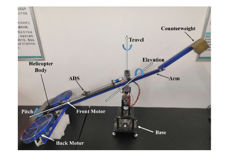
Because of the similar dynamics with the real helicopter system, the 3-DOF laboratory helicopter, as shown in Figure 1, can act as an ideal experimental platform for testing various advanced control methods of the helicopter [3]. In recent years, researchers have proposed numerous methods to achieve the attitude tracking object of 3-DOF helicopter and verified these methods by the helicopter experimental platform. These methods can be mainly divided into three parts: linear control [4, 5], nonlinear control [6, 7, 2, 8, 9] and intelligent control [10, 11, 12].
Refer to caption
Figure 1: Structure of 3-DOF helicopter system with ADS

Among all the above-mentioned control methods, sliding mode control has attracted much attention because of its insensitivity and strong robustness to the disturbances. In the present sliding mode algorithms, the super-twisting algorithm is very popular and owns practical application value due to the features of finite-time convergence, strong robustness and solely requiring the information of sliding mode variables [13]. In [14], a fast super-twisting algorithm is proposed to solve the problem that the convergence speed becomes slow when the system states are far away from their equilibrium points existing in [13]. However, the bound of disturbance needing to be known in advance restricts the applications of these super-twisting algorithms. To deal with this problem, an adaptive super-twisting algorithm is proposed in [15], which can adapt to the disturbance of unknown boundary. Combining the merits of [14] and [15], an adaptive fast second-order sliding mode control method is proposed in [16]. An observer is also designed in the light of this method, but the output of the proposed observer is not smooth. In [17], a smooth second-order sliding mode control is proposed to further alleviate the chattering effect existing in [13]. In [18], a fast smooth second-order sliding mode method is present based on the method of [17]. However, this method cannot adapt to the unknown boundary disturbances. Considering all the above-mentioned modified super-twisting methods, there is no method that can simultaneously achieve fast finite-time convergence, adaptation to the disturbances and smooth as of now.

In this paper, inspired by [16, 18], we propose a class of smooth adaptive fast second-order sliding mode control (SAFSOSMC) method and the method in [16] can be regarded as a special case of our proposed method to some extent. The new proposed method integrates the advantages of all the modified super-twisting algorithms mentioned before, including fast finite-time convergence, adaptation to the disturbances and smooth. To the best of the authors’ knowledge, this is the first time that a modified super-twisting algorithm can simultaneously own the above three merits. Based on this new method, a novel adaptive-gain smooth second-order sliding mode observer (ASSOSMO) is also proposed to alleviate chattering effect and adjust the parameters automatically without knowing the boundary of the lumped disturbances derivative. The main contributions of this paper can be summarized as follows:

  1. 1)

    A novel SAFSOSMC method is proposed to enable elevation and pitch angles to track given desired trajectories respectively, which not only maintains the characteristics of fast finite-time convergence and adaptation to the disturbance of unknown boundary, but also enormously reduces the chattering effect. Combined with a non-singular integral sliding mode surface[19], this method can ensure the fast finite-time convergence of the tracking errors with constant disturbances and the fast finite-time uniformly ultimately boundedness with the time-varying lumped disturbances.

  2. 2)

    A novel ASSOSMO is proposed to estimate the time-varying lumped disturbances of helicopter system control channels with smoother output than that of the adaptive-gain second-order sliding mode observer (ASOSMO) proposed in [16].

The fast finite-time convergence of the closed-loop system with constant disturbances and the fast finite-time uniformly ultimately boundedness of the closed-loop system with time-varying lumped disturbances will be proved with the corresponding finite-time Lyapunov stability theory. The effectiveness and superiority of the proposed control methods are verified by comparative experiments.

The remainder of this paper is organized as follows. In Section 2, the dynamic model and control objective of the 3-DOF helicopter system, some essential lemmas and the new proposition are given. The controller design process and stability analysis of the closed-loop system are presented in Section 3. Section 4 provides contrastive experiment results and discussion. Section 5 concludes this paper.

Notation: In this paper, we use \left\|\cdot\right\| to denote the Euclidean norm of vectors and sign()sign{\mathop{\rm sign}\nolimits}(\cdot) to denote the standard signum function. Moreover, λmax()subscript𝜆{\lambda_{\max}}\left(\cdot\right) and λmin()subscript𝜆{\lambda_{\min}}\left(\cdot\right) are used to denote the maximum and minimum eigenvalues of a matrix, respectively.

II Problem formulation and preliminaries

II-A The dynamics of the 3-DOF Helicopter

As shown in Fig.1, the 3-DOF helicopter system studied in this paper has elevation, pitch and travel motions, which are driven by two DC motors called the front motor and back motor. A positive voltage applied to each motor can generate the elevation motion, and a higher voltage applied on the front motor can produce the positive pitch motion . The travel motion can be generated by thrust vectors when the helicopter body is pitching. Moreover, an active disturbance system (ADS) serving as the lumped disturbances is installed on the arm.

Due to the under-actuated mechanism of the 3-DOF helicopter system, only two of the three degree of freedoms can be controlled to track arbitrary trajectories in the operating domain. In this work, we investigate the elevation and pitch motions, while the travel motion is set to move freely. The models of elevation and pitch channels can be expressed as follows [2]

Jαα¨subscript𝐽𝛼¨𝛼\displaystyle{J_{\alpha}}\ddot{\alpha} =KfLacos(β)(Vf+Vb)mgLacos(α)absentsubscript𝐾𝑓subscript𝐿𝑎𝛽subscript𝑉𝑓subscript𝑉𝑏𝑚𝑔subscript𝐿𝑎𝛼\displaystyle={K_{f}}{L_{a}}\cos(\beta)({V_{f}}+{V_{b}})-mg{L_{a}}\cos(\alpha) (1)
Jββ¨subscript𝐽𝛽¨𝛽\displaystyle{J_{\beta}}\ddot{\beta} =KfLh(VfVb)absentsubscript𝐾𝑓subscript𝐿subscript𝑉𝑓subscript𝑉𝑏\displaystyle={K_{f}}{L_{h}}({V_{f}}-{V_{b}})

where α𝛼\alpha and β𝛽\beta represent the elevation and pitch angle respectively. Taking into account the mechanical constraints, the operating domain of the helicopter system is defined as follows

27.5oα+30osuperscript27.5𝑜𝛼superscript30𝑜\displaystyle-{27.5^{o}}\leq\alpha\leq+{30^{o}} (2)
45oβ+45osuperscript45𝑜𝛽superscript45𝑜\displaystyle-{45^{o}}\leq\beta\leq+{45^{o}}

The definitions and values of the relevant parameters are shown in Table I.

TABLE I: The parameters of the 3-DOF helicopter system
Symbol Definition Value
Jαsubscript𝐽𝛼{J_{\alpha}} Moment of inertia of elevation axis 1.0348kgm21.0348𝑘𝑔superscript𝑚21.0348kg\cdot m^{2}
Jβsubscript𝐽𝛽{J_{\beta}} Moment of inertia of pitch axis 0.0451kgm20.0451𝑘𝑔superscript𝑚20.0451kg\cdot m^{2}
\pbox20cmLasubscript𝐿𝑎{L_{a}}
\pbox20cmDistance from elevation axis to the center
of helicopter body \pbox20cm0.6600m0.6600𝑚0.6600m
Lhsubscript𝐿{L_{h}} Distance from pitch axis to either motor 0.1780m0.1780𝑚0.1780m
m𝑚{m} Effective mass of the helicopter 0.094kg0.094𝑘𝑔0.094kg
g𝑔{g} Gravitational acceleration constant 9.81m/s29.81𝑚superscript𝑠29.81m/s^{2}
Kfsubscript𝐾𝑓{K_{f}} Propeller force-thrust constant 0.1188N/V0.1188𝑁𝑉0.1188N/V
Vfsubscript𝑉𝑓{V_{f}} Front motor voltage input [24,24]V2424𝑉[-24,24]V
Vbsubscript𝑉𝑏{V_{b}} Back motor voltage input [24,24]V2424𝑉[-24,24]V

Denote x1=α,x2=α˙,x3=β,x4=β˙formulae-sequencesubscript𝑥1𝛼formulae-sequencesubscript𝑥2˙𝛼formulae-sequencesubscript𝑥3𝛽subscript𝑥4˙𝛽{x_{1}}=\alpha,{x_{2}}=\dot{\alpha},{x_{3}}=\beta,{x_{4}}=\dot{\beta}. In view of the external disturbance and system uncertainty, the model of helicopter system can be rewritten as

x˙1subscript˙𝑥1\displaystyle{{\dot{x}}_{1}} =x2absentsubscript𝑥2\displaystyle={x_{2}} (3)
x˙2subscript˙𝑥2\displaystyle{{\dot{x}}_{2}} =LaJαcos(x3)u1gJαmLacos(x1)+d1(x)absentsubscript𝐿𝑎subscript𝐽𝛼subscript𝑥3subscript𝑢1𝑔subscript𝐽𝛼𝑚subscript𝐿𝑎subscript𝑥1subscript𝑑1𝑥\displaystyle=\frac{{{L_{a}}}}{{{J_{\alpha}}}}\cos({x_{3}}){u_{1}}-\frac{g}{{{J_{\alpha}}}}m{L_{a}}\cos({x_{1}})+{d_{1}}(x)
x˙3subscript˙𝑥3\displaystyle{{\dot{x}}_{3}} =x4absentsubscript𝑥4\displaystyle={x_{4}}
x˙4subscript˙𝑥4\displaystyle{{\dot{x}}_{4}} =LhJβu2+d2(x)absentsubscript𝐿subscript𝐽𝛽subscript𝑢2subscript𝑑2𝑥\displaystyle=\frac{{{L_{h}}}}{{{J_{\beta}}}}{u_{2}}+{d_{2}}(x)

where x=[x1,x2,x3,x4]T𝑥superscriptsubscript𝑥1subscript𝑥2subscript𝑥3subscript𝑥4𝑇x={[{x_{1}},{x_{2}},{x_{3}},{x_{4}}]^{T}} denotes the state vector of system (1), which is assumed to be measurable in this study. d1(x)subscript𝑑1𝑥{d_{1}}\left(x\right) and d2(x)subscript𝑑2𝑥{d_{2}}\left(x\right) represent the lumped disturbances existing in the corresponding control channels. In addition, u1subscript𝑢1{u_{1}}and u2subscript𝑢2{u_{2}} are defined by

u1subscript𝑢1\displaystyle{u_{1}} =Kf(Vf+Vb)absentsubscript𝐾𝑓subscript𝑉𝑓subscript𝑉𝑏\displaystyle={K_{f}}({V_{f}}+{V_{b}}) (4)
u2subscript𝑢2\displaystyle{u_{2}} =Kf(VfVb)absentsubscript𝐾𝑓subscript𝑉𝑓subscript𝑉𝑏\displaystyle={K_{f}}({V_{f}}-{V_{b}})

The control objective is to design the controllers such that the elevation and pitch angles can track the given desired trajectories respectively within small errors in finite time. For the design of the controllers, the following assumptions are required.

Assumption 1

The lumped disturbances and their first derivative are assumed to be bounded, while the value of the bound is unknown, i.e., there exist unknown constants d¯1subscript¯𝑑1{\overline{d}_{1}}, δ1subscript𝛿1\delta_{1}, d¯2subscript¯𝑑2{\overline{d}_{2}}, δ2subscript𝛿2\delta_{2} such that |d1(x)|d¯1subscript𝑑1𝑥subscript¯𝑑1\left|{{d_{1}}\left(x\right)}\right|\leq{\overline{d}_{1}}, |d˙1(x)|δ1subscript˙𝑑1𝑥subscript𝛿1\left|{{{\dot{d}}_{1}}\left(x\right)}\right|\leq{\delta_{1}}, |d2(x)|d¯2subscript𝑑2𝑥subscript¯𝑑2\left|{{d_{2}}\left(x\right)}\right|\leq{\overline{d}_{2}} and |d˙2(x)|δ2subscript˙𝑑2𝑥subscript𝛿2\left|{{{\dot{d}}_{2}}\left(x\right)}\right|\leq{\delta_{2}}, where d¯1>0,δ10,d¯2>0,δ20formulae-sequencesubscript¯𝑑10formulae-sequencesubscript𝛿10formulae-sequencesubscript¯𝑑20subscript𝛿20{\overline{d}_{1}}>0,{\delta_{1}}\geq 0,{\overline{d}_{2}}>0,{\delta_{2}}\geq 0

Assumption 2

The desired trajectories given by xαd(t)subscript𝑥𝛼𝑑𝑡{x_{\alpha d}}(t), xβd(t)subscript𝑥𝛽𝑑𝑡{x_{\beta d}}(t) are assumed to be bounded and available up to their second derivative.

II-B Definitions and Lemmas

To better describe the following definitions and lemmas, we consider a general system

x˙=g(x(t)),x0=x(0)formulae-sequence˙𝑥𝑔𝑥𝑡subscript𝑥0𝑥0\dot{x}=g(x(t)),{x_{0}}=x(0) (5)

where g:W0Rn:𝑔subscript𝑊0superscript𝑅𝑛g:{W_{0}}\to{R^{n}} is continuous on an open neighborhood W0Rnsubscript𝑊0superscript𝑅𝑛{W_{0}}\subset{R^{n}} of the origin and assume that g(0)=0𝑔00g(0)=0. x(t,x0)𝑥𝑡subscript𝑥0x(t,{x_{0}}) denote the solution of (5), which is in the sense of Filippov [20].

Definition 1 ([21])

If the origin of (5) is Lyapunov stable and any solution of (5) converges to the equilibrium point in finite time, i.e. x0W1W0for-allsubscript𝑥0subscript𝑊1subscript𝑊0\forall{x_{0}}\in{W_{1}}\subset{W_{0}}, x(t,x0)W1\{0}𝑥𝑡subscript𝑥0\subscript𝑊10x(t,{x_{0}})\in{W_{1}}\backslash\left\{0\right\} when t[0,T(x0)]𝑡0𝑇subscript𝑥0t\in[0,T({x_{0}})] with limtT(x0)x(t,x0)=0subscript𝑡𝑇subscript𝑥0𝑥𝑡subscript𝑥00{\lim_{t\to T({x_{0}})}}x(t,{x_{0}})=0, and x(t,x0)=0𝑥𝑡subscript𝑥00x(t,{x_{0}})=0 t>T(x0)for-all𝑡𝑇subscript𝑥0\forall t>T({x_{0}}), where T:W1\{0}(0,):𝑇\subscript𝑊100T:{W_{1}}\backslash\left\{0\right\}\to(0,\infty) is a continuous function, then the system (5) is called finite-time stable.

Definition 2 ([22])

If any solution of (5) converges to a neighborhood of the origin in finite time, the system (5) is called finite-time uniformly ultimately boundedness.

Lemma 1 ([23])

Suppose there exists a continuous and positive-definite function V:W0R:𝑉subscript𝑊0𝑅V:{W_{0}}\to R satisfying the condition

V˙(x)c1V(x)pc2V(x)˙𝑉𝑥subscript𝑐1𝑉superscript𝑥𝑝subscript𝑐2𝑉𝑥\dot{V}(x)\leq-{c_{1}}V{(x)^{p}}-{c_{2}}V(x) (6)

where c1>0,c2>0,p(0,1)formulae-sequencesubscript𝑐10formulae-sequencesubscript𝑐20𝑝01{c_{1}}>0,{c_{2}}>0,p\in(0,1), then the trajectory of (5) is fast finite-time stable. Moreover, the settling time is given by:

Tln[1+c2V(x0)1p/c1]c2(1p)𝑇1subscript𝑐2𝑉superscriptsubscript𝑥01𝑝subscript𝑐1subscript𝑐21𝑝T\leq\frac{{\ln[1+{c_{2}}V{{({x_{0}})}^{1-p}}/{c_{1}}]}}{{{c_{2}}(1-p)}} (7)
Lemma 2 ([18])

Suppose there exists a continuous and positive-definite function V:W0R:𝑉subscript𝑊0𝑅V:{W_{0}}\to R satisfying the condition

V˙(x)c1V(x)p1c2V(x)+c3V(x)p2˙𝑉𝑥subscript𝑐1𝑉superscript𝑥subscript𝑝1subscript𝑐2𝑉𝑥subscript𝑐3𝑉superscript𝑥subscript𝑝2\dot{V}(x)\leq-{c_{1}}V{(x)^{{p_{1}}}}-{c_{2}}V(x){\rm{+}}{c_{3}}V{(x)^{{p_{2}}}} (8)

where c1>0,c2>0,c3>0,p1(0,1),p2(0,p1)formulae-sequencesubscript𝑐10formulae-sequencesubscript𝑐20formulae-sequencesubscript𝑐30formulae-sequencesubscript𝑝101subscript𝑝20subscript𝑝1{c_{1}}>0,{c_{2}}>0,{c_{3}}>0,{p_{1}}\in(0,1),{p_{2}}\in(0,{p_{1}}), then the trajectory of (5) is fast finite-time uniformly ultimately boundedness. Moreover, the settling time is given by:

Tln[1+(c2θ2)V(x0)1p1/(c1θ1)](c2θ2)(1p1)𝑇1subscript𝑐2subscript𝜃2𝑉superscriptsubscript𝑥01subscript𝑝1subscript𝑐1subscript𝜃1subscript𝑐2subscript𝜃21subscript𝑝1T\leq\frac{{\ln[1+({c_{2}}-{\theta_{2}})V{{({x_{0}})}^{1-{p_{1}}}}/({c_{1}}-{\theta_{1}})]}}{{({c_{2}}-{\theta_{2}})(1-{p_{1}})}} (9)

where θ1subscript𝜃1{\theta_{1}} and θ2subscript𝜃2{\theta_{2}} are arbitrary positive constants holding θ1(0,c1),θ2(0,c2)formulae-sequencesubscript𝜃10subscript𝑐1subscript𝜃20subscript𝑐2{\theta_{1}}\in(0,{c_{1}}),{\theta_{2}}\in(0,{c_{2}}), then x(t,x0)𝑥𝑡subscript𝑥0x(t,{x_{0}}) can converge to a neighborhood of origin in a finite time T𝑇T. In addition, the convergent region can be given by:

D={x:θ1V(x)p1p2+θ2V(x)1p2<c3}𝐷conditional-set𝑥subscript𝜃1𝑉superscript𝑥subscript𝑝1subscript𝑝2subscript𝜃2𝑉superscript𝑥1subscript𝑝2subscript𝑐3D=\left\{{x:{\theta_{1}}V{{(x)}^{{p_{1}}-{p_{2}}}}+{\theta_{2}}V{{(x)}^{1-{p_{2}}}}<{c_{3}}}\right\} (10)

Define an auxiliary variable θ3(0,1)subscript𝜃301{\theta_{3}}\in\left({0,1}\right). If θ3subscript𝜃3{\theta_{3}} is selected satisfying

θ31p2θ2p1p2c31p2=θ11p2(1θ3)p1p2superscriptsubscript𝜃31subscript𝑝2superscriptsubscript𝜃2subscript𝑝1subscript𝑝2superscriptsubscript𝑐31subscript𝑝2superscriptsubscript𝜃11subscript𝑝2superscript1subscript𝜃3subscript𝑝1subscript𝑝2{\theta_{3}}^{1-{p_{2}}}{\theta_{2}}^{{p_{1}}-{p_{2}}}{c_{3}}^{1-{p_{2}}}={\theta_{1}}^{1-{p_{2}}}{(1-{\theta_{3}})^{{p_{1}}-{p_{2}}}} (11)

then (10) can be reduced to D=D1=D2𝐷subscript𝐷1subscript𝐷2D={D_{1}}={D_{2}}, where

D1subscript𝐷1\displaystyle{D_{1}} ={x:V(x)p1p2<θ3c3/θ1}absentconditional-set𝑥𝑉superscript𝑥subscript𝑝1subscript𝑝2subscript𝜃3subscript𝑐3subscript𝜃1\displaystyle=\left\{{x:V{{(x)}^{{p_{1}}-{p_{2}}}}<{\theta_{3}}{c_{3}}/{\theta_{1}}}\right\} (12)
D2subscript𝐷2\displaystyle{D_{2}} ={x:V(x)1p2<(1θ3)c3/θ2}absentconditional-set𝑥𝑉superscript𝑥1subscript𝑝21subscript𝜃3subscript𝑐3subscript𝜃2\displaystyle=\left\{{x:V{{(x)}^{1-{p_{2}}}}<\left({1-{\theta_{3}}}\right){c_{3}}/{\theta_{2}}}\right\}

which means the state x𝑥x can converge to D1=D2subscript𝐷1subscript𝐷2{D_{1}}={D_{2}} in finite time T𝑇T.

Remark 1

The meaning of fast in Lemma 1 and Lemma 2 is that the solution of (5) can quickly converge to the origin or a neighborhood of the origin regardless of the distance between the initial state and the origin, while the original finite-time stable converges slowly when the initial state is far away from the origin.

Lemma 3 ([19])

Considering the following system

x˙1subscript˙𝑥1\displaystyle{{\dot{x}}_{1}} =x2absentsubscript𝑥2\displaystyle={x_{2}} (13)
x˙2subscript˙𝑥2\displaystyle{{\dot{x}}_{2}} =γ1|x1|p3sgn(x1)γ2|x2|2p3/(1+p3)sgn(x2)absentsubscript𝛾1superscriptsubscript𝑥1subscript𝑝3sgnsubscript𝑥1subscript𝛾2superscriptsubscript𝑥22subscript𝑝31subscript𝑝3sgnsubscript𝑥2\displaystyle=-{\gamma_{1}}{\left|{{x_{1}}}\right|^{{p_{3}}}}{\mathop{\rm sgn}}({x_{1}})-{\gamma_{2}}{\left|{{x_{2}}}\right|^{2{p_{3}}/(1+{p_{3}})}}{\mathop{\rm sgn}}({x_{2}})

where γ1>0,γ2>0,p3(0,1)formulae-sequencesubscript𝛾10formulae-sequencesubscript𝛾20subscript𝑝301{\gamma_{1}}>0,{\gamma_{2}}>0,{p_{3}}\in(0,1), the trajectory of the system (13) is finite-time stable, i.e. x1,x2subscript𝑥1subscript𝑥2x_{1},x_{2} can converge to the origin in finite time.

II-C A New Proposition

Motivated by [18], we extend the result in [16] to obtain the following new proposition and this generalization is non-trivial.

Proposition 1

Considering the following system

s˙˙𝑠\displaystyle\dot{s} =L1(t)|s|m1msgn(s)L2(t)s+φabsentsubscript𝐿1𝑡superscript𝑠𝑚1𝑚sgn𝑠subscript𝐿2𝑡𝑠𝜑\displaystyle=-{L_{1}}(t){\left|s\right|^{\frac{{m-1}}{m}}}{\mathop{\rm sgn}}(s)-{L_{2}}(t)s+\varphi (14)
φ˙˙𝜑\displaystyle\dot{\varphi} =L3(t)|s|m2msgn(s)L4(t)s+d(t)absentsubscript𝐿3𝑡superscript𝑠𝑚2𝑚sgn𝑠subscript𝐿4𝑡𝑠𝑑𝑡\displaystyle=-{L_{3}}(t){\left|s\right|^{\frac{{m-2}}{m}}}{\mathop{\rm sgn}}(s)-{L_{4}}(t)s+d\left(t\right)

where |d(t)|δ𝑑𝑡𝛿\left|{d\left(t\right)}\right|\leq\delta, δ𝛿\delta is an unknown non-negative constant and the adaptive gains L1(t),L2(t),L3(t),L4(t)subscript𝐿1𝑡subscript𝐿2𝑡subscript𝐿3𝑡subscript𝐿4𝑡{L_{1}}(t),{L_{2}}(t),{L_{3}}(t),{L_{4}}(t) are expressed as

L1(t)subscript𝐿1𝑡\displaystyle{L_{1}}(t) =k1L0m1m(t),L2(t)=k2L0(t)formulae-sequenceabsentsubscript𝑘1superscriptsubscript𝐿0𝑚1𝑚𝑡subscript𝐿2𝑡subscript𝑘2subscript𝐿0𝑡\displaystyle={k_{1}}L_{0}^{{\textstyle{{m-1}\over m}}}\left(t\right),{\rm{}}{L_{2}}(t)={k_{2}}L_{0}\left(t\right) (15)
L3(t)subscript𝐿3𝑡\displaystyle{L_{3}}(t) =k3L02m2m(t),L4(t)=k4L02(t)formulae-sequenceabsentsubscript𝑘3superscriptsubscript𝐿02𝑚2𝑚𝑡subscript𝐿4𝑡subscript𝑘4superscriptsubscript𝐿02𝑡\displaystyle={k_{3}}L_{0}^{{\textstyle{{2m-2}\over m}}}\left(t\right),{\rm{}}{L_{4}}(t)={k_{4}}L_{0}^{2}\left(t\right)

where k1,k2,k3,k4,msubscript𝑘1subscript𝑘2subscript𝑘3subscript𝑘4𝑚{k_{1}},{k_{2}},{k_{3}},{k_{4}},m are positive constants satisfying

m2k3k4>(m3k3m1+(4m24m+1)k12)k22,m>2formulae-sequencesuperscript𝑚2subscript𝑘3subscript𝑘4superscript𝑚3subscript𝑘3𝑚14superscript𝑚24𝑚1superscriptsubscript𝑘12superscriptsubscript𝑘22𝑚2{m^{2}}{k_{3}}{k_{4}}>\left({\frac{{{m^{3}}{k_{3}}}}{{m-1}}+\left({4{m^{2}}-4m+1}\right){k_{1}}^{2}}\right){k_{2}}^{2},m>2 (16)

L0(t)subscript𝐿0𝑡{L_{0}}(t) is a scalar, positive, and time-varying function. The L0(t)subscript𝐿0𝑡{L_{0}}(t) satisfies

L0˙(t)={κ,if|s|ε0,else˙subscript𝐿0𝑡cases𝜅𝑖𝑓𝑠𝜀0𝑒𝑙𝑠𝑒\dot{L_{0}}\left(t\right)=\begin{cases}{\kappa},&if\quad\left|s\right|\geq\varepsilon\hfill\\ 0,&else\hfill\\ \end{cases} (17)

where κ𝜅\kappa is a positive constant, ε𝜀\varepsilon is an arbitrary small positive value. Then we can obtain the following conclusions

(i) If d=0𝑑0d=0, then s,s˙𝑠˙𝑠s,\dot{s} can fast converge to the origin in finite time.

(ii) If d0𝑑0d\neq 0, then s,s˙𝑠˙𝑠s,\dot{s} can fast converge to a neighborhood of the origin in finite time.

Proof:

Define a new state vector

ξ=[ξ1ξ2ξ3]=[L0m1m(t)|s|m1msgn(s)L0(t)sφ]𝜉delimited-[]subscript𝜉1missing-subexpressionmissing-subexpressionmissing-subexpressionmissing-subexpressionmissing-subexpressionmissing-subexpressionmissing-subexpressionmissing-subexpressionmissing-subexpressionmissing-subexpressionmissing-subexpressionmissing-subexpressionmissing-subexpressionmissing-subexpressionmissing-subexpressionmissing-subexpressionmissing-subexpressionmissing-subexpressionmissing-subexpressionsubscript𝜉2missing-subexpressionmissing-subexpressionmissing-subexpressionmissing-subexpressionmissing-subexpressionmissing-subexpressionmissing-subexpressionmissing-subexpressionmissing-subexpressionmissing-subexpressionmissing-subexpressionmissing-subexpressionmissing-subexpressionmissing-subexpressionmissing-subexpressionmissing-subexpressionmissing-subexpressionmissing-subexpressionmissing-subexpressionsubscript𝜉3missing-subexpressionmissing-subexpressionmissing-subexpressionmissing-subexpressionmissing-subexpressionmissing-subexpressionmissing-subexpressionmissing-subexpressionmissing-subexpressionmissing-subexpressionmissing-subexpressionmissing-subexpressionmissing-subexpressionmissing-subexpressionmissing-subexpressionmissing-subexpressionmissing-subexpressionmissing-subexpressionmissing-subexpressiondelimited-[]superscriptsubscript𝐿0𝑚1𝑚𝑡superscript𝑠𝑚1𝑚sgn𝑠missing-subexpressionmissing-subexpressionmissing-subexpressionmissing-subexpressionmissing-subexpressionmissing-subexpressionmissing-subexpressionmissing-subexpressionmissing-subexpressionmissing-subexpressionmissing-subexpressionmissing-subexpressionmissing-subexpressionmissing-subexpressionmissing-subexpressionmissing-subexpressionmissing-subexpressionmissing-subexpressionmissing-subexpressionsubscript𝐿0𝑡𝑠missing-subexpressionmissing-subexpressionmissing-subexpressionmissing-subexpressionmissing-subexpressionmissing-subexpressionmissing-subexpressionmissing-subexpressionmissing-subexpressionmissing-subexpressionmissing-subexpressionmissing-subexpressionmissing-subexpressionmissing-subexpressionmissing-subexpressionmissing-subexpressionmissing-subexpressionmissing-subexpressionmissing-subexpression𝜑missing-subexpressionmissing-subexpressionmissing-subexpressionmissing-subexpressionmissing-subexpressionmissing-subexpressionmissing-subexpressionmissing-subexpressionmissing-subexpressionmissing-subexpressionmissing-subexpressionmissing-subexpressionmissing-subexpressionmissing-subexpressionmissing-subexpressionmissing-subexpressionmissing-subexpressionmissing-subexpressionmissing-subexpression\xi=\left[{\begin{array}[]{*{20}{c}}{{\xi_{1}}}\\ {{\xi_{2}}}\\ {{\xi_{3}}}\end{array}}\right]=\left[{\begin{array}[]{*{20}{c}}{L_{0}^{{\textstyle{{m-1}\over m}}}\left(t\right){{\left|s\right|}^{{\textstyle{{m-1}\over m}}}}{\mathop{\rm sgn}}(s)}\\ {L_{0}\left(t\right)s}\\ \varphi\end{array}}\right] (18)

After taking the derivative of ξ𝜉\xi, we can obtain

ξ˙=˙𝜉absent\displaystyle\dot{\xi}= L0m1m|s|1m[m1mk1m1mk2m1m000k300]ξsuperscriptsubscript𝐿0𝑚1𝑚superscript𝑠1𝑚delimited-[]𝑚1𝑚subscript𝑘1𝑚1𝑚subscript𝑘2𝑚1𝑚missing-subexpressionmissing-subexpressionmissing-subexpressionmissing-subexpressionmissing-subexpressionmissing-subexpressionmissing-subexpressionmissing-subexpressionmissing-subexpressionmissing-subexpressionmissing-subexpressionmissing-subexpressionmissing-subexpressionmissing-subexpressionmissing-subexpressionmissing-subexpressionmissing-subexpression000missing-subexpressionmissing-subexpressionmissing-subexpressionmissing-subexpressionmissing-subexpressionmissing-subexpressionmissing-subexpressionmissing-subexpressionmissing-subexpressionmissing-subexpressionmissing-subexpressionmissing-subexpressionmissing-subexpressionmissing-subexpressionmissing-subexpressionmissing-subexpressionmissing-subexpressionsubscript𝑘300missing-subexpressionmissing-subexpressionmissing-subexpressionmissing-subexpressionmissing-subexpressionmissing-subexpressionmissing-subexpressionmissing-subexpressionmissing-subexpressionmissing-subexpressionmissing-subexpressionmissing-subexpressionmissing-subexpressionmissing-subexpressionmissing-subexpressionmissing-subexpressionmissing-subexpression𝜉\displaystyle L_{0}^{{\textstyle{{m-1}\over m}}}{\left|s\right|^{\frac{{-1}}{m}}}\left[{\begin{array}[]{*{20}{c}}{-\frac{{m-1}}{m}{k_{1}}}&{-\frac{{m-1}}{m}{k_{2}}}&{\frac{{m-1}}{m}}\\ 0&0&0\\ {-{k_{3}}}&0&0\end{array}}\right]\xi (19)
+L0[000k1k210k40]ξ+[m1mL˙0(t)L0(t)ξ1L˙0(t)L0(t)ξ2d(t)]subscript𝐿0delimited-[]000missing-subexpressionmissing-subexpressionmissing-subexpressionmissing-subexpressionmissing-subexpressionmissing-subexpressionmissing-subexpressionmissing-subexpressionmissing-subexpressionmissing-subexpressionmissing-subexpressionmissing-subexpressionmissing-subexpressionmissing-subexpressionmissing-subexpressionmissing-subexpressionmissing-subexpressionsubscript𝑘1subscript𝑘21missing-subexpressionmissing-subexpressionmissing-subexpressionmissing-subexpressionmissing-subexpressionmissing-subexpressionmissing-subexpressionmissing-subexpressionmissing-subexpressionmissing-subexpressionmissing-subexpressionmissing-subexpressionmissing-subexpressionmissing-subexpressionmissing-subexpressionmissing-subexpressionmissing-subexpression0subscript𝑘40missing-subexpressionmissing-subexpressionmissing-subexpressionmissing-subexpressionmissing-subexpressionmissing-subexpressionmissing-subexpressionmissing-subexpressionmissing-subexpressionmissing-subexpressionmissing-subexpressionmissing-subexpressionmissing-subexpressionmissing-subexpressionmissing-subexpressionmissing-subexpressionmissing-subexpression𝜉delimited-[]𝑚1𝑚subscript˙𝐿0𝑡subscript𝐿0𝑡subscript𝜉1missing-subexpressionmissing-subexpressionmissing-subexpressionmissing-subexpressionmissing-subexpressionmissing-subexpressionmissing-subexpressionmissing-subexpressionmissing-subexpressionmissing-subexpressionmissing-subexpressionmissing-subexpressionmissing-subexpressionmissing-subexpressionmissing-subexpressionmissing-subexpressionmissing-subexpressionmissing-subexpressionmissing-subexpressionsubscript˙𝐿0𝑡subscript𝐿0𝑡subscript𝜉2missing-subexpressionmissing-subexpressionmissing-subexpressionmissing-subexpressionmissing-subexpressionmissing-subexpressionmissing-subexpressionmissing-subexpressionmissing-subexpressionmissing-subexpressionmissing-subexpressionmissing-subexpressionmissing-subexpressionmissing-subexpressionmissing-subexpressionmissing-subexpressionmissing-subexpressionmissing-subexpressionmissing-subexpression𝑑𝑡missing-subexpressionmissing-subexpressionmissing-subexpressionmissing-subexpressionmissing-subexpressionmissing-subexpressionmissing-subexpressionmissing-subexpressionmissing-subexpressionmissing-subexpressionmissing-subexpressionmissing-subexpressionmissing-subexpressionmissing-subexpressionmissing-subexpressionmissing-subexpressionmissing-subexpressionmissing-subexpressionmissing-subexpression\displaystyle+L_{0}\left[{\begin{array}[]{*{20}{c}}0&0&0\\ {{\rm{-}}{k_{1}}}&{-{k_{2}}}&1\\ 0&{-{k_{4}}}&0\end{array}}\right]\xi+\left[{\begin{array}[]{*{20}{c}}{\frac{{m-1}}{m}\frac{{{{\dot{L}}_{0}}(t)}}{{{L_{0}}(t)}}{\xi_{1}}}\\ {\frac{{{{\dot{L}}_{0}}(t)}}{{{L_{0}}(t)}}{\xi_{2}}}\\ {d(t)}\end{array}}\right]

Then a candidate Lyapunov function is chosen as V(ξ)=ξTPξ𝑉𝜉superscript𝜉𝑇𝑃𝜉V\left(\xi\right)={\xi^{T}}P\xi, with

P=12[2mm1k3+k12k1k2k1k1k22k4+k22k2k1k22]𝑃12delimited-[]2𝑚𝑚1subscript𝑘3superscriptsubscript𝑘12subscript𝑘1subscript𝑘2subscript𝑘1missing-subexpressionmissing-subexpressionmissing-subexpressionmissing-subexpressionmissing-subexpressionmissing-subexpressionmissing-subexpressionmissing-subexpressionmissing-subexpressionmissing-subexpressionmissing-subexpressionmissing-subexpressionmissing-subexpressionmissing-subexpressionmissing-subexpressionmissing-subexpressionmissing-subexpressionsubscript𝑘1subscript𝑘22subscript𝑘4superscriptsubscript𝑘22subscript𝑘2missing-subexpressionmissing-subexpressionmissing-subexpressionmissing-subexpressionmissing-subexpressionmissing-subexpressionmissing-subexpressionmissing-subexpressionmissing-subexpressionmissing-subexpressionmissing-subexpressionmissing-subexpressionmissing-subexpressionmissing-subexpressionmissing-subexpressionmissing-subexpressionmissing-subexpressionsubscript𝑘1subscript𝑘22missing-subexpressionmissing-subexpressionmissing-subexpressionmissing-subexpressionmissing-subexpressionmissing-subexpressionmissing-subexpressionmissing-subexpressionmissing-subexpressionmissing-subexpressionmissing-subexpressionmissing-subexpressionmissing-subexpressionmissing-subexpressionmissing-subexpressionmissing-subexpressionmissing-subexpression\displaystyle P=\frac{1}{2}\left[{\begin{array}[]{*{20}{c}}{\frac{{2m}}{{m-1}}{k_{3}}+{k_{1}}^{2}}&{{k_{1}}{k_{2}}}&{-{k_{1}}}\\ {{k_{1}}{k_{2}}}&{2{k_{4}}+{k_{2}}^{2}}&{-{k_{2}}}\\ {-{k_{1}}}&{-{k_{2}}}&2\end{array}}\right] (20)

where P𝑃P is a symmetric positive definite matrix. Taking the derivative of V(ξ)𝑉𝜉V\left(\xi\right) along the trajectories of system (14) yields

V˙(ξ)=˙𝑉𝜉absent\displaystyle\dot{V}\left(\xi\right)= L0|ξ1|1m1ξTΩ1ξL0ξTΩ2ξsubscript𝐿0superscriptsubscript𝜉11𝑚1superscript𝜉𝑇subscriptΩ1𝜉subscript𝐿0superscript𝜉𝑇subscriptΩ2𝜉\displaystyle-{L_{0}}{\left|{{\xi_{1}}}\right|^{{\textstyle{{-1}\over{m-1}}}}}{\xi^{T}}{\Omega_{1}}\xi-L_{0}{\xi^{T}}{\Omega_{2}}\xi (21)
+σ1d(t)ξ+2m2mL˙0(t)L0(t)σ2Pξsubscript𝜎1𝑑𝑡𝜉2𝑚2𝑚subscript˙𝐿0𝑡subscript𝐿0𝑡subscript𝜎2𝑃𝜉\displaystyle+{\sigma_{1}}d\left(t\right)\xi+\frac{{2m-2}}{m}\frac{{{{\dot{L}}_{0}}(t)}}{{{L_{0}}(t)}}{\sigma_{2}}P\xi

where σ1=[k1k22]subscript𝜎1subscript𝑘1subscript𝑘22\sigma_{1}=\left[-k_{1}-k_{2}\quad 2\right], σ2=[ξ1mm1ξ20]subscript𝜎2subscript𝜉1𝑚𝑚1subscript𝜉20\sigma_{2}=\left[\xi_{1}\quad\frac{m}{m-1}{\xi_{2}}\quad 0\right] and

Ω1=subscriptΩ1absent\displaystyle{\Omega_{1}}= (22)
k1m[k3m+k12(m1)0k1(m1)0k4m+k22(3m1)k2(2m1)k1(m1)k2(2m1)m1]subscript𝑘1𝑚delimited-[]subscript𝑘3𝑚superscriptsubscript𝑘12𝑚10subscript𝑘1𝑚1missing-subexpressionmissing-subexpressionmissing-subexpressionmissing-subexpressionmissing-subexpressionmissing-subexpressionmissing-subexpressionmissing-subexpressionmissing-subexpressionmissing-subexpressionmissing-subexpressionmissing-subexpressionmissing-subexpressionmissing-subexpressionmissing-subexpressionmissing-subexpressionmissing-subexpression0subscript𝑘4𝑚superscriptsubscript𝑘223𝑚1subscript𝑘22𝑚1missing-subexpressionmissing-subexpressionmissing-subexpressionmissing-subexpressionmissing-subexpressionmissing-subexpressionmissing-subexpressionmissing-subexpressionmissing-subexpressionmissing-subexpressionmissing-subexpressionmissing-subexpressionmissing-subexpressionmissing-subexpressionmissing-subexpressionmissing-subexpressionmissing-subexpressionsubscript𝑘1𝑚1subscript𝑘22𝑚1𝑚1missing-subexpressionmissing-subexpressionmissing-subexpressionmissing-subexpressionmissing-subexpressionmissing-subexpressionmissing-subexpressionmissing-subexpressionmissing-subexpressionmissing-subexpressionmissing-subexpressionmissing-subexpressionmissing-subexpressionmissing-subexpressionmissing-subexpressionmissing-subexpressionmissing-subexpression\displaystyle\frac{{{k_{1}}}}{m}\left[{\begin{array}[]{*{20}{c}}{{k_{3}}m+k_{1}^{2}\left({m-1}\right)}&0&{-{k_{1}}\left({m-1}\right)}\\ 0&{{k_{4}}m+k_{2}^{2}\left({3m-1}\right)}&{-{k_{2}}\left({2m-1}\right)}\\ {-{k_{1}}\left({m-1}\right)}&{-{k_{2}}\left({2m-1}\right)}&{m-1}\end{array}}\right]
Ω2=k2[k3+k12(3m2)/m000k4+k22k20k21]subscriptΩ2subscript𝑘2delimited-[]subscript𝑘3superscriptsubscript𝑘123𝑚2𝑚00missing-subexpressionmissing-subexpressionmissing-subexpressionmissing-subexpressionmissing-subexpressionmissing-subexpressionmissing-subexpressionmissing-subexpressionmissing-subexpressionmissing-subexpressionmissing-subexpressionmissing-subexpressionmissing-subexpressionmissing-subexpressionmissing-subexpressionmissing-subexpressionmissing-subexpression0subscript𝑘4superscriptsubscript𝑘22subscript𝑘2missing-subexpressionmissing-subexpressionmissing-subexpressionmissing-subexpressionmissing-subexpressionmissing-subexpressionmissing-subexpressionmissing-subexpressionmissing-subexpressionmissing-subexpressionmissing-subexpressionmissing-subexpressionmissing-subexpressionmissing-subexpressionmissing-subexpressionmissing-subexpressionmissing-subexpression0subscript𝑘21missing-subexpressionmissing-subexpressionmissing-subexpressionmissing-subexpressionmissing-subexpressionmissing-subexpressionmissing-subexpressionmissing-subexpressionmissing-subexpressionmissing-subexpressionmissing-subexpressionmissing-subexpressionmissing-subexpressionmissing-subexpressionmissing-subexpressionmissing-subexpressionmissing-subexpression\displaystyle{\Omega_{2}}={k_{2}}\left[{\begin{array}[]{*{20}{c}}{{k_{3}}+k_{1}^{2}\left({3m-2}\right)/m}&0&0\\ 0&{{k_{4}}+k_{2}^{2}}&{-{k_{2}}}\\ 0&{-{k_{2}}}&1\end{array}}\right]

It is easy to prove that the matrices Ω1subscriptΩ1\Omega_{1} and Ω2subscriptΩ2\Omega_{2} both are positive definite with (16). By using

λmin(P)ξ2Vλmax(P)ξ2subscript𝜆𝑃superscriptnorm𝜉2𝑉subscript𝜆𝑃superscriptnorm𝜉2{\lambda_{\min}}\left(P\right){\left\|\xi\right\|^{2}}\leq V\leq{\lambda_{\max}}\left(P\right){\left\|\xi\right\|^{2}} (23)

(21) can be formulated as

V˙˙𝑉absent\displaystyle\dot{V}\leq L0(t)λmin(Ω1)λmaxp1(P)Vp1L0(t)λmin(Ω2)λmax(P)Vsubscript𝐿0𝑡subscript𝜆subscriptΩ1superscriptsubscript𝜆subscript𝑝1𝑃superscript𝑉subscript𝑝1subscript𝐿0𝑡subscript𝜆subscriptΩ2subscript𝜆𝑃𝑉\displaystyle-{L_{0}}\left(t\right)\frac{{{\lambda_{\min}}\left({{\Omega_{1}}}\right)}}{{\lambda_{\max}^{{p_{1}}}\left(P\right)}}{V^{{p_{1}}}}-L_{0}\left(t\right)\frac{{{\lambda_{\min}}\left({{\Omega_{2}}}\right)}}{{{\lambda_{\max}}\left(P\right)}}V (24)
+δσ12λmin1/2(P)V12+m1mL˙0L0ξTQξ𝛿subscriptnormsubscript𝜎12superscriptsubscript𝜆12𝑃superscript𝑉12𝑚1𝑚subscript˙𝐿0subscript𝐿0superscript𝜉𝑇𝑄𝜉\displaystyle+\frac{{\delta{{\left\|{{\sigma_{1}}}\right\|}_{2}}}}{{\lambda_{\min}^{{\raise 1.50694pt\hbox{$\scriptstyle 1$}\kern-0.70004pt/\kern-1.04996pt\lower 0.75346pt\hbox{$\scriptstyle 2$}}}\left(P\right)}}{V^{\frac{1}{2}}}+\frac{{m-1}}{m}\frac{{{{\dot{L}}_{0}}}}{{{L_{0}}}}{\xi^{T}}Q\xi

where p1=(2m3)/(2m2)subscript𝑝12𝑚32𝑚2{p_{1}}=\left({2m-3}\right)/\left({2m-2}\right), Q=diag[q1,q2,q3]𝑄𝑑𝑖𝑎𝑔subscript𝑞1subscript𝑞2subscript𝑞3Q=diag\left[{{q_{1}},{q_{2}},{q_{3}}}\right] is a diagonal matrix with positive diagonal elements, which are expressed as follows

q1subscript𝑞1\displaystyle{q_{1}} =2mm1k3+k12+(2m1)k1k22(m1)+k12absent2𝑚𝑚1subscript𝑘3superscriptsubscript𝑘122𝑚1subscript𝑘1subscript𝑘22𝑚1subscript𝑘12\displaystyle=\frac{{2m}}{{m-1}}{k_{3}}+k_{1}^{2}+\frac{{\left({2m-1}\right){k_{1}}{k_{2}}}}{{2\left({m-1}\right)}}+\frac{{{k_{1}}}}{2} (25)
q2subscript𝑞2\displaystyle{q_{2}} =m2(m1)(4k4+2k22+k2)+(2m1)k1k22(m1)absent𝑚2𝑚14subscript𝑘42superscriptsubscript𝑘22subscript𝑘22𝑚1subscript𝑘1subscript𝑘22𝑚1\displaystyle=\frac{m}{{2\left({m-1}\right)}}\left({4{k_{4}}+2k_{2}^{2}+{k_{2}}}\right)+\frac{{\left({2m-1}\right){k_{1}}{k_{2}}}}{{2\left({m-1}\right)}}
q3subscript𝑞3\displaystyle{q_{3}} =k12+mk22(m1)absentsubscript𝑘12𝑚subscript𝑘22𝑚1\displaystyle=\frac{{{k_{1}}}}{2}+\frac{{m{k_{2}}}}{{2\left({m-1}\right)}}

Then (24) can be further rewritten as

V˙L0(t)n1Vp1+n2V12(L0(t)n32m2mn4L˙0L0)V˙𝑉subscript𝐿0𝑡subscript𝑛1superscript𝑉subscript𝑝1subscript𝑛2superscript𝑉12subscript𝐿0𝑡subscript𝑛32𝑚2𝑚subscript𝑛4subscript˙𝐿0subscript𝐿0𝑉\small\dot{V}\leq-{L_{0}}\left(t\right){n_{1}}{V^{{p_{1}}}}+{n_{2}}{V^{\frac{1}{2}}}-\left({L_{0}\left(t\right){n_{3}}-\frac{{2m-2}}{m}{n_{4}}\frac{{{{\dot{L}}_{0}}}}{{{L_{0}}}}}\right)V (26)

where

n1subscript𝑛1\displaystyle{n_{1}} =λmin(Ω1)λmaxp1(P)absentsubscript𝜆subscriptΩ1superscriptsubscript𝜆subscript𝑝1𝑃\displaystyle=\frac{{{\lambda_{\min}}\left({{\Omega_{1}}}\right)}}{{\lambda_{\max}^{{p_{1}}}\left(P\right)}} (27)
n2subscript𝑛2\displaystyle{n_{2}} =δσ12λmin1/2(P)absent𝛿subscriptnormsubscript𝜎12superscriptsubscript𝜆12𝑃\displaystyle=\frac{{\delta{{\left\|{{\sigma_{1}}}\right\|}_{2}}}}{{\lambda_{\min}^{{\raise 1.50694pt\hbox{$\scriptstyle 1$}\kern-0.70004pt/\kern-1.04996pt\lower 0.75346pt\hbox{$\scriptstyle 2$}}}\left(P\right)}}
n3subscript𝑛3\displaystyle{n_{3}} =λmin(Ω2)λmax(P)absentsubscript𝜆subscriptΩ2subscript𝜆𝑃\displaystyle=\frac{{{\lambda_{\min}}\left({{\Omega_{2}}}\right)}}{{{\lambda_{\max}}\left(P\right)}}
n4subscript𝑛4\displaystyle{n_{4}} =λmax(Q)2λmin(P)absentsubscript𝜆𝑄2subscript𝜆𝑃\displaystyle=\frac{{{\lambda_{\max}}\left(Q\right)}}{{2{\lambda_{\min}}\left(P\right)}}

(i) If d(t)=0𝑑𝑡0d(t)=0, then δ=0𝛿0\delta=0, (26) will become

V˙L0(t)n1Vp1(L0(t)n32m2mn4L˙0L0)V˙𝑉subscript𝐿0𝑡subscript𝑛1superscript𝑉subscript𝑝1subscript𝐿0𝑡subscript𝑛32𝑚2𝑚subscript𝑛4subscript˙𝐿0subscript𝐿0𝑉\dot{V}\leq-{L_{0}}\left(t\right){n_{1}}{V^{{p_{1}}}}-\left({L_{0}\left(t\right){n_{3}}-\frac{{2m-2}}{m}{n_{4}}\frac{{{{\dot{L}}_{0}}}}{{{L_{0}}}}}\right)V (28)

Due to L˙0(t)0subscript˙𝐿0𝑡0{\dot{L}_{0}}\left(t\right)\geq 0, L0(t)n3(2m2)n4L˙0/(L0m)subscript𝐿0𝑡subscript𝑛32𝑚2subscript𝑛4subscript˙𝐿0subscript𝐿0𝑚L_{0}\left(t\right){n_{3}}-\left({2m-2}\right){n_{4}}{\dot{L}_{0}}/\left({{L_{0}}m}\right) is positive in finite time. It follows from (28) that

V˙c1Vp1c2V˙𝑉subscript𝑐1superscript𝑉subscript𝑝1subscript𝑐2𝑉\dot{V}\leq-{c_{1}}{V^{{p_{1}}}}-{c_{2}}V (29)

where c1subscript𝑐1{c_{1}} and c2subscript𝑐2{c_{2}} are positive constants, p1(0.5,1)subscript𝑝10.51{p_{1}}\in(0.5,1). By using Lemma 1, ξ𝜉\xi can fast converge to origin in finite time, then s,s˙𝑠˙𝑠s,\dot{s} can fast converge to the origin in finite time.

(ii) If d(t)0𝑑𝑡0d\left(t\right)\neq 0, with the same analysis of (i), it follows from (26) that

V˙c4Vp1c5V+c3V12˙𝑉subscript𝑐4superscript𝑉subscript𝑝1subscript𝑐5𝑉subscript𝑐3superscript𝑉12\dot{V}\leq-{c_{4}}{V^{{p_{1}}}}-{c_{5}}V{\rm{+}}{c_{3}}{V^{{\textstyle{1\over 2}}}} (30)

where c3,c4subscript𝑐3subscript𝑐4{c_{3}},{c_{4}}and c5subscript𝑐5{c_{5}} are positive constants, p1(0.5,1)subscript𝑝10.51{p_{1}}\in(0.5,1). By using Lemma 2, ξ𝜉\xi can fast converge to a neighborhood of origin in finite time. In addition, the region can be given by

D={ξ:θ1V(ξ)p1p2+θ2V(ξ)1p2<c3}𝐷conditional-set𝜉subscript𝜃1𝑉superscript𝜉subscript𝑝1subscript𝑝2subscript𝜃2𝑉superscript𝜉1subscript𝑝2subscript𝑐3D=\left\{{\xi:{\theta_{1}}V{{(\xi)}^{{p_{1}}-{p_{2}}}}+{\theta_{2}}V{{(\xi)}^{1-{p_{2}}}}<{c_{3}}}\right\} (31)

where θ1(0,c4),θ2(0,c5)formulae-sequencesubscript𝜃10subscript𝑐4subscript𝜃20subscript𝑐5{\theta_{1}}\in(0,{c_{4}}),{\theta_{2}}\in(0,{c_{5}}), p2=0.5subscript𝑝20.5{p_{2}}=0.5.

Define an auxiliary variable θ3(0,1)subscript𝜃301{\theta_{3}}\in\left({0,1}\right).If θ3subscript𝜃3{\theta_{3}} is selected satisfying

θ31p2θ2p1p2c31p2=θ11p2(1θ3)p1p2superscriptsubscript𝜃31subscript𝑝2superscriptsubscript𝜃2subscript𝑝1subscript𝑝2superscriptsubscript𝑐31subscript𝑝2superscriptsubscript𝜃11subscript𝑝2superscript1subscript𝜃3subscript𝑝1subscript𝑝2{\theta_{3}}^{1-{p_{2}}}{\theta_{2}}^{{p_{1}}-{p_{2}}}{c_{3}}^{1-{p_{2}}}={\theta_{1}}^{1-{p_{2}}}{(1-{\theta_{3}})^{{p_{1}}-{p_{2}}}} (32)

ξ𝜉\xi can converge to D=D1=D2𝐷subscript𝐷1subscript𝐷2D={D_{1}}={D_{2}} in finite time T1subscript𝑇1{T_{1}}, where

T1ln[1+(c5θ2)V(ξ0)1p1/(c4θ1)](c5θ2)(1p1)subscript𝑇11subscript𝑐5subscript𝜃2𝑉superscriptsubscript𝜉01subscript𝑝1subscript𝑐4subscript𝜃1subscript𝑐5subscript𝜃21subscript𝑝1{T_{1}}\leq\frac{{\ln[1+({c_{5}}-{\theta_{2}})V{{({\xi_{0}})}^{1-{p_{1}}}}/({c_{4}}-{\theta_{1}})]}}{{({c_{5}}-{\theta_{2}})(1-{p_{1}})}} (33)
D1={ξ:V(ξ)p1p2<θ3c3/θ1}D2={ξ:V(ξ)1p2<(1θ3)c3/θ2}subscript𝐷1conditional-set𝜉𝑉superscript𝜉subscript𝑝1subscript𝑝2subscript𝜃3subscript𝑐3subscript𝜃1subscript𝐷2conditional-set𝜉𝑉superscript𝜉1subscript𝑝21subscript𝜃3subscript𝑐3subscript𝜃2\displaystyle\begin{array}[]{l}{D_{1}}=\left\{{\xi:V{{(\xi)}^{{p_{1}}-{p_{2}}}}<{\theta_{3}}{c_{3}}/{\theta_{1}}}\right\}\\ {D_{2}}=\left\{{\xi:V{{(\xi)}^{1-{p_{2}}}}<\left({1-{\theta_{3}}}\right){c_{3}}/{\theta_{2}}}\right\}\end{array} (34)

Design a region D4subscript𝐷4D_{4} as

D4subscript𝐷4\displaystyle{D_{4}} ={ξ:λmin(P)ξ2<(1θ3)2c32/θ22}absentconditional-set𝜉subscript𝜆𝑃superscriptnorm𝜉2superscript1subscript𝜃32superscriptsubscript𝑐32superscriptsubscript𝜃22\displaystyle=\left\{{\xi:{\lambda_{\min}}\left(P\right){{\left\|\xi\right\|}^{2}}<{{\left({1-{\theta_{3}}}\right)}^{2}}c_{3}^{2}/{\theta_{2}}^{2}}\right\} (35)
={ξ:ξ<Δ}absentconditional-set𝜉norm𝜉Δ\displaystyle=\left\{{\xi:\left\|\xi\right\|<{\Delta}}\right\}

where Δ=λmin(P)1/2(1θ3)c3/θ2Δsubscript𝜆superscript𝑃121subscript𝜃3subscript𝑐3subscript𝜃2{\Delta}{\rm{=}}{\lambda_{\min}}{\left(P\right)^{-1/2}}\left({1-{\theta_{3}}}\right){c_{3}}/{\theta_{2}}. In terms of (23), it follows from (34) and (35) that D4subscript𝐷4D_{4} contains D2subscript𝐷2D_{2}. Considering the definition of ξ𝜉\xi, the following inequalities ξ1ξnormsubscript𝜉1norm𝜉\left\|{{\xi_{1}}}\right\|\leq\left\|\xi\right\|, ξ2ξnormsubscript𝜉2norm𝜉\left\|{{\xi_{2}}}\right\|\leq\left\|\xi\right\|and ξ3ξnormsubscript𝜉3norm𝜉\left\|{{\xi_{3}}}\right\|\leq\left\|\xi\right\| hold. Then the set

D5={ξ1,ξ2,ξ3:ξ1<Δ,ξ2<Δ,ξ3<Δ}subscript𝐷5conditional-setsubscript𝜉1subscript𝜉2subscript𝜉3formulae-sequencenormsubscript𝜉1Δformulae-sequencenormsubscript𝜉2Δnormsubscript𝜉3Δ{D_{5}}=\left\{{{\xi_{1}},{\xi_{2}},{\xi_{3}}:\left\|{{\xi_{1}}}\right\|<{\Delta},\left\|{{\xi_{2}}}\right\|<{\Delta},\left\|{{\xi_{3}}}\right\|<{\Delta}}\right\} (36)

contains the set D4subscript𝐷4D_{4}. Therefore, since ξ𝜉\xi converges to D1subscript𝐷1D_{1} in T1subscript𝑇1T_{1} , it will also converge to D5subscript𝐷5D_{5} in T1subscript𝑇1T_{1} . Using (14), (15) and (18), we can obtain that s,s˙𝑠˙𝑠s,\dot{s} converge to a neighborhood of the origin in T1subscript𝑇1T_{1}. ∎

Remark 2

By selecting different values of m𝑚m in (14), we can obtain a series of smooth adaptive fast second-order sliding mode control methods and if m=2𝑚2m=2, (14) can be transformed into the result in [16]. However, our proposed methods can greatly reduce the chattering effect existing in [16]. The newly proposed proposition will be used in the design of controller and observer for the helicopter system in the next section, and the superiority of our proposed control method will be verified through the comparative simulation experiments.

III Controller and Observer Design

In this section, we will give the design process of controller and observer in detail. First, the system (3) is transformed into the tracking error system. Then a control scheme, consisting of a non-singular integral sliding mode surface and a novel SAFSOSMC method, is proposed for the tracking error system subject to constant disturbance and time-varying lumped disturbance. Finally, a novel ASSOSMO is present to estimate disturbances.

III-A System transformation

Defining the tracking errors e1=x1xαd(t),e2=x2x˙αd(t),e3=x3xβd(t),e4=x4x˙βd(t)formulae-sequencesubscript𝑒1subscript𝑥1subscript𝑥𝛼𝑑𝑡formulae-sequencesubscript𝑒2subscript𝑥2subscript˙𝑥𝛼𝑑𝑡formulae-sequencesubscript𝑒3subscript𝑥3subscript𝑥𝛽𝑑𝑡subscript𝑒4subscript𝑥4subscript˙𝑥𝛽𝑑𝑡{e_{1}}={x_{1}}-{x_{\alpha d}}(t),{e_{2}}={x_{2}}-{\dot{x}_{\alpha d}}(t),{e_{3}}={x_{3}}-{x_{\beta d}}(t),{e_{4}}={x_{4}}-{\dot{x}_{\beta d}}(t). Then the tracking error system is given by

e˙1subscript˙𝑒1\displaystyle{\dot{e}_{1}} =e2absentsubscript𝑒2\displaystyle={e_{2}} (37)
e˙2subscript˙𝑒2\displaystyle{\dot{e}_{2}} =LaJαcos(x3)u1gJαmLacos(x1)x¨αd(t)+d1(x)absentsubscript𝐿𝑎subscript𝐽𝛼subscript𝑥3subscript𝑢1𝑔subscript𝐽𝛼𝑚subscript𝐿𝑎subscript𝑥1subscript¨𝑥𝛼𝑑𝑡subscript𝑑1𝑥\displaystyle=\frac{{{L_{a}}}}{{{J_{\alpha}}}}\cos({x_{3}}){u_{1}}-\frac{g}{{{J_{\alpha}}}}m{L_{a}}\cos({x_{1}})-{\ddot{x}_{\alpha d}}(t)+{d_{1}}(x)
e˙3subscript˙𝑒3\displaystyle{\dot{e}_{3}} =e4absentsubscript𝑒4\displaystyle={e_{4}}
e˙4subscript˙𝑒4\displaystyle{\dot{e}_{4}} =LhJβu2x¨βd(t)+d2(x)absentsubscript𝐿subscript𝐽𝛽subscript𝑢2subscript¨𝑥𝛽𝑑𝑡subscript𝑑2𝑥\displaystyle=\frac{{{L_{h}}}}{{{J_{\beta}}}}{u_{2}}-{\ddot{x}_{\beta d}}(t)+{d_{2}}(x)

The control objective is then transformed into the design of finite-time controller so that e1subscript𝑒1{e_{1}} and e3subscript𝑒3{e_{3}} can converge to the origin or a small region of the origin. To facilitate the design of controllers, we express the models of the elevation and pitch channels in a unified form

e˙i=ei+1subscript˙𝑒𝑖subscript𝑒𝑖1\displaystyle{\dot{e}_{i}}={e_{i+1}} (38)
e˙i+1=givi+fi+disubscript˙𝑒𝑖1subscript𝑔𝑖subscript𝑣𝑖subscript𝑓𝑖subscript𝑑𝑖\displaystyle{\dot{e}_{i+1}}={g_{i}}{v_{i}}+{f_{i}}+{d_{i}}

where fisubscript𝑓𝑖{f_{i}} and gi,i=1,2formulae-sequencesubscript𝑔𝑖𝑖12{g_{i}},i=1,2 represent the dynamics of corresponding channels, which can be express as follows

f1subscript𝑓1\displaystyle{f_{1}} =gJαmLacos(x1)x¨αd(t)absent𝑔subscript𝐽𝛼𝑚subscript𝐿𝑎subscript𝑥1subscript¨𝑥𝛼𝑑𝑡\displaystyle=-\frac{g}{{{J_{\alpha}}}}m{L_{a}}\cos({x_{1}})-{{\ddot{x}}_{\alpha d}}(t) (39)
g1subscript𝑔1\displaystyle{g_{1}} =LaJαabsentsubscript𝐿𝑎subscript𝐽𝛼\displaystyle=\frac{{{L_{a}}}}{{{J_{\alpha}}}}
f2subscript𝑓2\displaystyle{f_{2}} =x¨βd(t)absentsubscript¨𝑥𝛽𝑑𝑡\displaystyle=-{{\ddot{x}}_{\beta d}}(t)
g2subscript𝑔2\displaystyle{g_{2}} =LhJβabsentsubscript𝐿subscript𝐽𝛽\displaystyle=\frac{{{L_{h}}}}{{{J_{\beta}}}}

and the auxiliary control inputs v1subscript𝑣1{v_{1}} and v2subscript𝑣2{v_{2}} are defined as

v1subscript𝑣1\displaystyle{v_{1}} =cos(x3)u1absentsubscript𝑥3subscript𝑢1\displaystyle=\cos({x_{3}}){u_{1}} (40)
v2subscript𝑣2\displaystyle{v_{2}} =u2absentsubscript𝑢2\displaystyle={u_{2}}

Then, we will take the elevation channel as an example to expound the design process and the controller for the pitch channel can be designed following a similar process. Afterwards, we can get the auxiliary control inputs v1subscript𝑣1{v_{1}} and v2subscript𝑣2{v_{2}}. By using (4) and (40), we can easily obtain the true control inputs Vfsubscript𝑉𝑓{V_{f}} andVbsubscript𝑉𝑏{V_{b}}.

III-B Controller design with constant disturbance

Considering the tracking error system of the elevation channel

e˙1=e2subscript˙𝑒1subscript𝑒2\displaystyle{{\dot{e}}_{1}}={e_{2}} (41)
e˙2=g1v1+f1+d1subscript˙𝑒2subscript𝑔1subscript𝑣1subscript𝑓1subscript𝑑1\displaystyle{{\dot{e}}_{2}}={g_{1}}{v_{1}}+{f_{1}}+{d_{1}}

where d1subscript𝑑1{d_{1}} is constant disturbance, i.e. d˙1=0subscript˙𝑑10{\dot{d}_{1}}=0. We adopt a non-singular integral sliding mode surface from [19], which is defined as follows

s=e2+0tz𝑑τ𝑠subscript𝑒2superscriptsubscript0𝑡𝑧differential-d𝜏s={e_{2}}+\int_{0}^{t}{zd\tau} (42)

where z=γ3|e1|p4sgn(e1)+γ4|e2|2p4/(1+p4)sgn(e2)𝑧subscript𝛾3superscriptsubscript𝑒1subscript𝑝4sgnsubscript𝑒1subscript𝛾4superscriptsubscript𝑒22subscript𝑝41subscript𝑝4sgnsubscript𝑒2z={\gamma_{3}}{\left|{{e_{1}}}\right|^{{p_{4}}}}{\mathop{\rm sgn}}({e_{1}})+{\gamma_{4}}{\left|{{e_{2}}}\right|^{2{p_{4}}/(1+{p_{4}})}}{\mathop{\rm sgn}}({e_{2}}) and γ3>0,γ4>0,p4(0,1)formulae-sequencesubscript𝛾30formulae-sequencesubscript𝛾40subscript𝑝401{\gamma_{3}}>0,{\gamma_{4}}>0,{p_{4}}\in(0,1).

Based on this sliding mode variable and Proposition 1, a novel smooth adaptive fast second-order sliding mode controller can be designed as

v1=subscript𝑣1absent\displaystyle{v_{1}}= g11{L1(t)|s|m1msgn(s)L2(t)sz\displaystyle{g_{1}}^{-1}\left\{{-{L_{1}}(t){{\left|s\right|}^{\frac{{m-1}}{m}}}{\mathop{\rm sgn}}(s)-{L_{2}}(t)s-z}\right. (43)
f10t[L3(t)|s|m2msgn(s)+L4(t)s]dτ}\displaystyle\phantom{=\;\;}\left.{-{f_{1}}-\int_{0}^{t}{\left[{{L_{3}}(t){{\left|s\right|}^{\frac{{m-2}}{m}}}{\mathop{\rm sgn}}(s)+{L_{4}}(t)s}\right]d\tau}}\right\}

where L1(t),L2(t),L3(t),L4(t)subscript𝐿1𝑡subscript𝐿2𝑡subscript𝐿3𝑡subscript𝐿4𝑡{L_{1}}(t),{L_{2}}(t),{L_{3}}(t),{L_{4}}(t) are formulated the same as (15) and m>2𝑚2m>2.

Theorem 1

Considering the tracking error system (41) subject to constant disturbance, the proposed control law (43) ensures that the tracking error can fast converge to the origin in finite time.

Proof:

We will adopt two steps to complete the proof. In Step 1, we will prove that the s˙˙𝑠\dot{s} can fast converge to the origin in finite time. In Step 2, we prove that the tracking error e1subscript𝑒1e_{1} will converge to the origin in finite time when s˙=0˙𝑠0\dot{s}=0 .

Step 1. Taking the derivative of (42),we can obtain

s˙=e˙2+z˙𝑠subscript˙𝑒2𝑧\dot{s}={\dot{e}_{2}}+z (44)

Substituting (41) and (43) into (44) leads to

s˙=˙𝑠absent\displaystyle\dot{s}= L1(t)|s|m1msgn(s)L2(t)s+d1subscript𝐿1𝑡superscript𝑠𝑚1𝑚sgn𝑠subscript𝐿2𝑡𝑠subscript𝑑1\displaystyle-{L_{1}}(t){\left|s\right|^{\frac{{m-1}}{m}}}{\mathop{\rm sgn}}(s)-{L_{2}}(t)s+{d_{1}} (45)
0t[L3(t)|s|m2msgn(s)+L4(t)s]𝑑τsuperscriptsubscript0𝑡delimited-[]subscript𝐿3𝑡superscript𝑠𝑚2𝑚sgn𝑠subscript𝐿4𝑡𝑠differential-d𝜏\displaystyle-\int_{0}^{t}{\left[{{L_{3}}(t){{\left|s\right|}^{\frac{{m-2}}{m}}}{\mathop{\rm sgn}}(s)+{L_{4}}(t)s}\right]d\tau}

We define an intermediate variable

φ=0t[L3(t)|s|m2msgn(s)+L4(t)s]𝑑τ+d1𝜑superscriptsubscript0𝑡delimited-[]subscript𝐿3𝑡superscript𝑠𝑚2𝑚sgn𝑠subscript𝐿4𝑡𝑠differential-d𝜏subscript𝑑1\varphi=-\int_{0}^{t}{\left[{{L_{3}}(t){{\left|s\right|}^{\frac{{m-2}}{m}}}{\mathop{\rm sgn}}(s)+{L_{4}}(t)s}\right]d\tau+}{d_{1}} (46)

Then (45) becomes

s˙=L1(t)|s|m1msgn(s)L2(t)s+φ˙𝑠subscript𝐿1𝑡superscript𝑠𝑚1𝑚sgn𝑠subscript𝐿2𝑡𝑠𝜑\displaystyle\dot{s}=-{L_{1}}(t){\left|s\right|^{\frac{{m-1}}{m}}}{\mathop{\rm sgn}}(s)-{L_{2}}(t)s+\varphi (47)
φ˙=L3(t)|s|m2msgn(s)L4(t)s˙𝜑subscript𝐿3𝑡superscript𝑠𝑚2𝑚sgn𝑠subscript𝐿4𝑡𝑠\displaystyle\dot{\varphi}=-{L_{3}}(t){\left|s\right|^{\frac{{m-2}}{m}}}{\mathop{\rm sgn}}(s)-{L_{4}}(t)s

By using Proposition 1, s˙˙𝑠\dot{s} can fast converge to the origin in finite time.

Step 2. When s˙=0˙𝑠0\dot{s}=0, (44) becomes

e˙2=γ3|e1|p4sgn(e1)γ4|e2|2p4/(1+p4)sgn(e2)subscript˙𝑒2subscript𝛾3superscriptsubscript𝑒1subscript𝑝4sgnsubscript𝑒1subscript𝛾4superscriptsubscript𝑒22subscript𝑝41subscript𝑝4sgnsubscript𝑒2{\dot{e}_{2}}=-{\gamma_{3}}{\left|{{e_{1}}}\right|^{{p_{4}}}}{\mathop{\rm sgn}}({e_{1}})-{\gamma_{4}}{\left|{{e_{2}}}\right|^{2{p_{4}}/(1+{p_{4}})}}{\mathop{\rm sgn}}({e_{2}}) (48)

By using Lemma 3 coupled with system (41), e1subscript𝑒1e_{1} and e2subscript𝑒2e_{2} can converge to the origin in finite time. The proof is completed. ∎

III-C Controller design with time-varying lumped disturbance

Considering the tracking error system of the elevation channel

e˙1=e2subscript˙𝑒1subscript𝑒2\displaystyle{{\dot{e}}_{1}}={e_{2}} (49)
e˙2=g1v1+f1+d1subscript˙𝑒2subscript𝑔1subscript𝑣1subscript𝑓1subscript𝑑1\displaystyle{{\dot{e}}_{2}}={g_{1}}{v_{1}}+{f_{1}}+{d_{1}}

where d1subscript𝑑1{d_{1}} is time-varying lumped disturbance satisfying Assumption 1, i.e. |d˙1|δ1,δ1>0formulae-sequencesubscript˙𝑑1subscript𝛿1subscript𝛿10\left|{{{\dot{d}}_{1}}}\right|\leq{\delta_{1}},{\delta_{1}}>0. We adopt the same non-singular integral sliding mode surface as (42), which is defined as follows

sv=e2+0tzv𝑑τsubscript𝑠𝑣subscript𝑒2superscriptsubscript0𝑡subscript𝑧𝑣differential-d𝜏{s_{v}}={e_{2}}+\int_{0}^{t}{{z_{v}}d\tau} (50)

where zv=γ5|e1|p5sgn(e1)+γ6|e2|2p5/(1+p5)sgn(e2)subscript𝑧𝑣subscript𝛾5superscriptsubscript𝑒1subscript𝑝5sgnsubscript𝑒1subscript𝛾6superscriptsubscript𝑒22subscript𝑝51subscript𝑝5sgnsubscript𝑒2{z_{v}}={\gamma_{5}}{\left|{{e_{1}}}\right|^{{p_{5}}}}{\mathop{\rm sgn}}({e_{1}})+{\gamma_{6}}{\left|{{e_{2}}}\right|^{2{p_{5}}/(1+{p_{5}})}}{\mathop{\rm sgn}}({e_{2}}) and γ5>0,γ6>0,p5(0,1)formulae-sequencesubscript𝛾50formulae-sequencesubscript𝛾60subscript𝑝501{\gamma_{5}}>0,{\gamma_{6}}>0,{p_{5}}\in(0,1).

Based on this sliding mode variable and Proposition 1, a novel smooth adaptive fast second-order sliding mode controller can be designed as

v1=subscript𝑣1absent\displaystyle{v_{1}}= g11{Lv1(t)|sv|m1msgn(sv)Lv2(t)svzv\displaystyle{g_{1}}^{-1}\left\{{-{L_{v1}}(t){{\left|{{s_{v}}}\right|}^{\frac{{m-1}}{m}}}{\mathop{\rm sgn}}({s_{v}})-{L_{v2}}(t){s_{v}}-{z_{v}}}\right. (51)
f10t[Lv3(t)|sv|m2msgn(sv)+Lv4(t)sv]dτ}\displaystyle\phantom{=\;\;}\left.{-{f_{1}}-\int_{0}^{t}{\left[{{L_{v}}_{3}(t){{\left|{{s_{v}}}\right|}^{\frac{{m-2}}{m}}}{\mathop{\rm sgn}}({s_{v}})+{L_{v4}}(t){s_{v}}}\right]d\tau}}\right\}

where Lv1(t),Lv2(t),Lv3(t),Lv4(t)subscript𝐿𝑣1𝑡subscript𝐿𝑣2𝑡subscript𝐿𝑣3𝑡subscript𝐿𝑣4𝑡{L_{v1}}(t),{L_{v2}}(t),{L_{v3}}(t),{L_{v4}}(t) are formulated the same as (15) and m>2𝑚2m>2.

Theorem 2

Considering the tracking error system (49) subject to time-varying lumped disturbance, the proposed control law (51) guarantees that the tracking error can fast converge to a region of the origin in finite time.

Proof:

We will adopt two steps to complete the proof. In Step 1, we will prove that the s˙˙𝑠\dot{s} can fast converge to a neighborhood of the origin in finite time. In Step 2, we prove that the tracking error e1subscript𝑒1e_{1} will converge to a neighborhood of the origin in finite time when |s˙v|Δ1subscript˙𝑠𝑣subscriptΔ1\left|{{{\dot{s}}_{v}}}\right|\leq\Delta_{1}.

Step 1. Taking the derivative of (50),we can obtain

s˙v=e˙2+zvsubscript˙𝑠𝑣subscript˙𝑒2subscript𝑧𝑣{\dot{s}_{v}}={\dot{e}_{2}}+{z_{v}} (52)

Substituting (49) and (51) into (52) leads to

s˙v=subscript˙𝑠𝑣absent\displaystyle{\dot{s}_{v}}= Lv1(t)|sv|m1msgn(sv)Lv2(t)sv+d1subscript𝐿𝑣1𝑡superscriptsubscript𝑠𝑣𝑚1𝑚sgnsubscript𝑠𝑣subscript𝐿𝑣2𝑡subscript𝑠𝑣subscript𝑑1\displaystyle-{L_{v1}}(t){\left|{{s_{v}}}\right|^{\frac{{m-1}}{m}}}{\mathop{\rm sgn}}({s_{v}})-{L_{v2}}(t){s_{v}}+{d_{1}} (53)
0t[Lv3(t)|sv|m2msgn(sv)+Lv4(t)sv]𝑑τsuperscriptsubscript0𝑡delimited-[]subscript𝐿𝑣3𝑡superscriptsubscript𝑠𝑣𝑚2𝑚sgnsubscript𝑠𝑣subscript𝐿𝑣4𝑡subscript𝑠𝑣differential-d𝜏\displaystyle-\int_{0}^{t}{\left[{{L_{v3}}(t){{\left|{{s_{v}}}\right|}^{\frac{{m-2}}{m}}}{\mathop{\rm sgn}}({s_{v}})+{L_{v4}}(t){s_{v}}}\right]d\tau}

We define an intermediate variable

φv=0t[Lv3(t)|sv|m2msgn(sv)+Lv4(t)sv]𝑑τ+d1subscript𝜑𝑣superscriptsubscript0𝑡delimited-[]subscript𝐿𝑣3𝑡superscriptsubscript𝑠𝑣𝑚2𝑚sgnsubscript𝑠𝑣subscript𝐿𝑣4𝑡subscript𝑠𝑣differential-d𝜏subscript𝑑1{\varphi_{v}}=-\int_{0}^{t}{\left[{{L_{v3}}(t){{\left|{{s_{v}}}\right|}^{\frac{{m-2}}{m}}}{\mathop{\rm sgn}}({s_{v}})+{L_{v4}}(t){s_{v}}}\right]d\tau+}{d_{1}} (54)

Then (53) becomes

s˙v=Lv1(t)|sv|m1msgn(sv)Lv2(t)sv+φvsubscript˙𝑠𝑣subscript𝐿𝑣1𝑡superscriptsubscript𝑠𝑣𝑚1𝑚sgnsubscript𝑠𝑣subscript𝐿𝑣2𝑡subscript𝑠𝑣subscript𝜑𝑣\displaystyle{{\dot{s}}_{v}}=-{L_{v1}}(t){\left|{{s_{v}}}\right|^{\frac{{m-1}}{m}}}{\mathop{\rm sgn}}({s_{v}})-{L_{v2}}(t){s_{v}}+{\varphi_{v}} (55)
φ˙v=Lv3(t)|sv|m2msgn(sv)Lv4(t)sv+d˙1subscript˙𝜑𝑣subscript𝐿𝑣3𝑡superscriptsubscript𝑠𝑣𝑚2𝑚sgnsubscript𝑠𝑣subscript𝐿𝑣4𝑡subscript𝑠𝑣subscript˙𝑑1\displaystyle{{\dot{\varphi}}_{v}}=-{L_{v3}}(t){\left|{{s_{v}}}\right|^{\frac{{m-2}}{m}}}{\mathop{\rm sgn}}({s_{v}})-{L_{v4}}(t){s_{v}}+{{\dot{d}}_{1}}

According to Assumption 1, the disturbance |d˙1|δ1subscript˙𝑑1subscript𝛿1\left|{{{\dot{d}}_{1}}}\right|\leq{\delta_{1}}. By using Proposition 1, s˙vsubscript˙𝑠𝑣{\dot{s}_{v}} can fast converge to a neighborhood of the origin in finite time, and the region is defined as Δ1subscriptΔ1\Delta_{1}.

Step 2. When |s˙v|Δ1subscript˙𝑠𝑣subscriptΔ1\left|{{{\dot{s}}_{v}}}\right|\leq\Delta_{1}, (52) becomes

e˙2+γ5|e1|p5sgn(e1)+γ6|e2|2p5/(1+p5)sgn(e2)=ϕsubscript˙𝑒2subscript𝛾5superscriptsubscript𝑒1subscript𝑝5sgnsubscript𝑒1subscript𝛾6superscriptsubscript𝑒22subscript𝑝51subscript𝑝5sgnsubscript𝑒2italic-ϕ{\dot{e}_{2}}+{\gamma_{5}}{\left|{{e_{1}}}\right|^{{p_{5}}}}{\mathop{\rm sgn}}({e_{1}})+{\gamma_{6}}{\left|{{e_{2}}}\right|^{2{p_{5}}/(1+{p_{5}})}}{\mathop{\rm sgn}}({e_{2}})=\phi (56)

where |ϕ|Δ1italic-ϕsubscriptΔ1\left|\phi\right|\leq\Delta_{1}.

Then (56) can be equivalently transformed into

e˙2+(γ5ϕ|e1|p5sgn(e1))|e1|p5sgn(e1)+γ6|e2|2p5/(1+p5)sgn(e2)=0subscript˙𝑒2subscript𝛾5italic-ϕsuperscriptsubscript𝑒1subscript𝑝5sgnsubscript𝑒1superscriptsubscript𝑒1subscript𝑝5sgnsubscript𝑒1subscript𝛾6superscriptsubscript𝑒22subscript𝑝51subscript𝑝5sgnsubscript𝑒20\small{\dot{e}_{2}}+\left({{\gamma_{5}}-\frac{\phi}{{{{\left|{{e_{1}}}\right|}^{{p_{5}}}}{\mathop{\rm sgn}}({e_{1}})}}}\right){\left|{{e_{1}}}\right|^{{p_{5}}}}{\mathop{\rm sgn}}({e_{1}})+{\gamma_{6}}{\left|{{e_{2}}}\right|^{2{p_{5}}/(1+{p_{5}})}}{\mathop{\rm sgn}}({e_{2}})=0 (57)

For (57), if γ5>|ϕ|/(|e1|p5sgn(e1))subscript𝛾5italic-ϕsuperscriptsubscript𝑒1subscript𝑝5sgnsubscript𝑒1\gamma_{5}>\left|\phi\right|/\left({{{\left|{{e_{1}}}\right|}^{{p_{5}}}}{\mathop{\rm sgn}}({e_{1}})}\right), then γ5ϕ/(|e1|p5sgn(e1))subscript𝛾5italic-ϕsuperscriptsubscript𝑒1subscript𝑝5sgnsubscript𝑒1{\gamma_{5}}-\phi/\left({{{\left|{{e_{1}}}\right|}^{{p_{5}}}}{\mathop{\rm sgn}}({e_{1}})}\right) will remain positive, and (57) is still kept in the form of (48). By using Lemma 3, the finite time converge of e1subscript𝑒1e_{1} is guaranteed, which also means that e1subscript𝑒1e_{1} can converge to the region |e1|(Δ1/γ5)1/p5subscript𝑒1superscriptsubscriptΔ1subscript𝛾51subscript𝑝5\left|{{e_{1}}}\right|\leq{\left({\Delta_{1}/{\gamma_{5}}}\right)^{1/{p_{5}}}}, i.e. the tracking error e1subscript𝑒1e_{1} will ultimately converge to the region |e1|(Δ1/γ5)1/p5subscript𝑒1superscriptsubscriptΔ1subscript𝛾51subscript𝑝5\left|{{e_{1}}}\right|\leq{\left({\Delta_{1}/{\gamma_{5}}}\right)^{1/{p_{5}}}} in finite time. The proof is completed. ∎

III-D The design of an observer

For the elevation control channel

e˙2=g1v1+f1+d1subscript˙𝑒2subscript𝑔1subscript𝑣1subscript𝑓1subscript𝑑1{\dot{e}_{2}}={g_{1}}{v_{1}}+{f_{1}}+{d_{1}} (58)

where d1subscript𝑑1{d_{1}} is a time-varying lumped disturbance satisfying Assumption 1. Then we will develop a novel sliding mode observer to estimate the disturbance based on Proposition 1, which is call adaptive-gain smooth second-order sliding mode observer (ASSOSMO).

First, an auxiliary estimation system is defined as

e^˙2=g1v1+f1+d^1subscript˙^𝑒2subscript𝑔1subscript𝑣1subscript𝑓1subscript^𝑑1{\dot{\hat{e}}_{2}}={g_{1}}{v_{1}}+{f_{1}}+{\hat{d}_{1}} (59)

Then a sliding mode variable is defined as

sd=e2e^2subscript𝑠𝑑subscript𝑒2subscript^𝑒2{s_{d}}={e_{2}}-{\hat{e}_{2}} (60)

Finally, the ASSOSMO can be designed as

d^1=Ld1(t)|sd|m1msgn(sd)+Ld2(t)sd+φdsubscript^𝑑1subscript𝐿𝑑1𝑡superscriptsubscript𝑠𝑑𝑚1𝑚sgnsubscript𝑠𝑑subscript𝐿𝑑2𝑡subscript𝑠𝑑subscript𝜑𝑑\displaystyle{{\hat{d}}_{1}}{\rm{=}}{L_{d1}}(t){\left|{{s_{d}}}\right|^{\frac{{m-1}}{m}}}{\mathop{\rm sgn}}({s_{d}})+{L_{d2}}(t){s_{d}}+{\varphi_{d}} (61)
φ˙d=Ld3(t)|sd|m2msgn(sd)+Ld4(t)sdsubscript˙𝜑𝑑subscript𝐿𝑑3𝑡superscriptsubscript𝑠𝑑𝑚2𝑚sgnsubscript𝑠𝑑subscript𝐿𝑑4𝑡subscript𝑠𝑑\displaystyle{{\dot{\varphi}}_{d}}={L_{d3}}(t){\left|{{s_{d}}}\right|^{\frac{{m-2}}{m}}}{\mathop{\rm sgn}}({s_{d}})+{L_{d4}}(t){s_{d}}

where L1d(t),L2d(t),L3d(t),L4d(t)subscript𝐿1𝑑𝑡subscript𝐿2𝑑𝑡subscript𝐿3𝑑𝑡subscript𝐿4𝑑𝑡{L_{1d}}(t),{L_{2d}}(t),{L_{3d}}(t),{L_{4d}}(t) are formulated the same as (15) and m>2𝑚2m>2.

Theorem 3

Under the condition of Assumption 1, the proposed observer (61) can guarantee that the estimation disturbance d^1subscript^𝑑1{\hat{d}_{1}} converges to a neighborhood of the true disturbance d1subscript𝑑1{d_{1}}.

Proof:

Taking the derivative of (60), we can obtain

s˙d=e˙2e^˙2=d1d^1subscript˙𝑠𝑑subscript˙𝑒2subscript˙^𝑒2subscript𝑑1subscript^𝑑1{\dot{s}_{d}}={\dot{e}_{2}}-{\dot{\hat{e}}_{2}}={d_{1}}-{\hat{d}_{1}} (62)

Substituting (61) into (62) leads to

s˙d=Ld1(t)|sd|m1msgn(sd)Ld2(t)sd+φd1subscript˙𝑠𝑑subscript𝐿𝑑1𝑡superscriptsubscript𝑠𝑑𝑚1𝑚sgnsubscript𝑠𝑑subscript𝐿𝑑2𝑡subscript𝑠𝑑subscript𝜑𝑑1\displaystyle{{\dot{s}}_{d}}=-{L_{d1}}(t){\left|{{s_{d}}}\right|^{\frac{{m-1}}{m}}}{\mathop{\rm sgn}}({s_{d}})-{L_{d2}}(t){s_{d}}+{\varphi_{d1}} (63)
φ˙d1=Ld3(t)|sd|m2msgn(sd)Ld4(t)sd+d˙1subscript˙𝜑𝑑1subscript𝐿𝑑3𝑡superscriptsubscript𝑠𝑑𝑚2𝑚sgnsubscript𝑠𝑑subscript𝐿𝑑4𝑡subscript𝑠𝑑subscript˙𝑑1\displaystyle{{\dot{\varphi}}_{d1}}=-{L_{d3}}(t){\left|{{s_{d}}}\right|^{\frac{{m-2}}{m}}}{\mathop{\rm sgn}}({s_{d}})-{L_{d4}}(t){s_{d}}+{{\dot{d}}_{1}}

In terms of Assumption 1, the disturbance |d˙1|δ1subscript˙𝑑1subscript𝛿1\left|{{{\dot{d}}_{1}}}\right|\leq{\delta_{1}}. Meanwhile, the L1d(t),L2d(t),L3d(t),L4d(t)subscript𝐿1𝑑𝑡subscript𝐿2𝑑𝑡subscript𝐿3𝑑𝑡subscript𝐿4𝑑𝑡{L_{1d}}(t),{L_{2d}}(t),{L_{3d}}(t),{L_{4d}}(t) are formulated the same as (15) and m>2𝑚2m>2. By using the Proposition 1, we can get that s˙dsubscript˙𝑠𝑑{\dot{s}_{d}} converges to a neighborhood of the origin. Then by using (62), the estimation disturbance d^1subscript^𝑑1{\hat{d}_{1}} can converge to a neighborhood of the true disturbance d1subscript𝑑1{d_{1}}, and the proof is accomplished.

Remark 3

The ASOSMO can also be developed following the same process by using the method in [16], which is selected as the comparing method. The effectiveness and smoothness of our proposed observer will be verified by the comparative simulation experiment.

IV Experimental Results

This section presents three sets of comparative simulation experiments to expound the effectiveness of our proposed control schemes. The AFSOSMC method proposed in [16], combined with an integral non-singular terminal sliding mode (INTSM) surface, is implemented as the comparison method, where the whole control scheme is proposed and analyzed in [24]. The INTSM-AFSOSMC method can be specifically expressed as follows

(i) An INTSM surface is selected as

sci=ei+1+0t|zci|13sgn(zci)dτsubscript𝑠𝑐𝑖subscript𝑒𝑖1superscriptsubscript0𝑡superscriptsubscript𝑧𝑐𝑖13sgnsubscript𝑧𝑐𝑖𝑑𝜏{s_{ci}}={e_{i+1}}+\int_{0}^{t}{{{\left|{{z_{ci}}}\right|}^{\frac{1}{3}}}{\mathop{\rm sgn}}({z_{ci}})d\tau} (64)

where zci=ei+|ei+1|32sgn(ei+1)subscript𝑧𝑐𝑖subscript𝑒𝑖superscriptsubscript𝑒𝑖132sgnsubscript𝑒𝑖1{z_{ci}}={e_{i}}+{\left|{{e_{i+1}}}\right|^{\frac{3}{2}}}{\mathop{\rm sgn}}({e_{i+1}})

(ii) The INTSM-AFSOSMC law is

uci=subscript𝑢𝑐𝑖absent\displaystyle u_{ci}= gi1{Lc1(t)|sci|12sgn(sci)Lc2(t)sci|zci|13sgn(zci)\displaystyle{g_{i}}^{-1}\left\{{-{L_{c1}}(t){{\left|{{s_{ci}}}\right|}^{\frac{1}{2}}}{\mathop{\rm sgn}}({s_{ci}})-{L_{c2}}(t){s_{ci}}-{{\left|{{z_{ci}}}\right|}^{\frac{1}{3}}}{\mathop{\rm sgn}}({z_{ci}})}\right. (65)
fi0t[Lc3(t)sgn(sci)+Lc4(t)sci]dτ}\displaystyle\phantom{=\;\;}\left.{-{f_{i}}-\int_{0}^{t}{\left[{{L_{c3}}(t){\mathop{\rm sgn}}({s_{ci}})+{L_{c4}}(t){s_{ci}}}\right]d\tau}}\right\}

where i=1,3𝑖13i=1,3 and the time-varying gains are defined the same as (15) with m=2𝑚2m=2.

Table I shows the parameter values of the helicopter system, and the fixed sampling time for all the simulation experiments is set to 0.001 second. In these experiments, the same initial position of the system starts from the elevation angle 24osuperscript24𝑜-24^{o} and pitch angle 0osuperscript0𝑜0^{o}. The desired trajectories of elevation angle and pitch angle are given as

xαd(t)=0.2sin(0.08tπ2),xβd(t)=0.1sin(0.06t)formulae-sequencesubscript𝑥𝛼𝑑𝑡0.20.08𝑡𝜋2subscript𝑥𝛽𝑑𝑡0.10.06𝑡{x_{\alpha d}}(t){\rm{=}}0.2\sin(0.08t-\frac{\pi}{2}),{x_{\beta d}}(t)=0.1\sin(0.06t) (66)

The purposes of three group experiments are summarized as follows

  1. 1)

    The first experiment shows the advantages of our control scheme for the attitude tracking of the helicopter system with constant disturbance by comparing with the control method in [24].

  2. 2)

    The second experiment demonstrates the merits of our control scheme for the attitude tracking of the helicopter system with time-varying disturbance, which is also compared with the control method in [24].

  3. 3)

    The third experiment is used to illustrate the smoother output of our proposed observer compared with the observer proposed from [16] in terms of estimating the time-varying lumped disturbances of the helicopter system.

IV-A Experiment I: Attitude tracking control with constant disturbance

For experiment I, the parameters of our proposed control scheme for elevation angle and pitch angle tracking are set as: γ1=γ2=5subscript𝛾1subscript𝛾25{\gamma_{1}}={\gamma_{2}}=5, p3=0.6subscript𝑝30.6{p_{3}}=0.6, m=3𝑚3m=3, k1=2subscript𝑘12{k_{1}}=2, k2subscript𝑘2{k_{2}} = 2.5, k3=4subscript𝑘34{k_{3}}=4, k4=30subscript𝑘430{k_{4}}=30, κ=5𝜅5\kappa=5. The INTSM-AFSOSMC law adopts the same gain parameters.
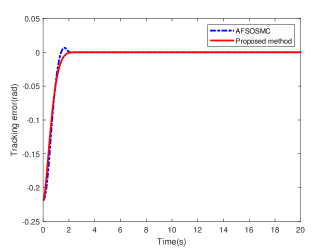
Refer to caption
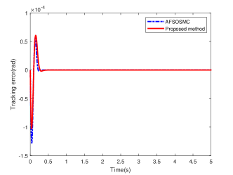
(a) Response of elevation tracking error by AFSOSMC and proposed method
Refer to caption
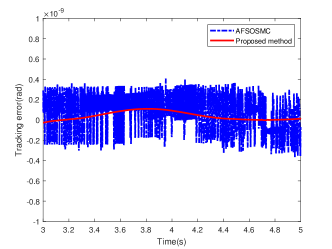
(b) Local magnification of elevation tracking error
Refer to caption
(c) Response of pitch tracking error by AFSOSMC and proposed method
Refer to caption
(d) Local magnification of pitch tracking error
Figure 2: Results of experiment I

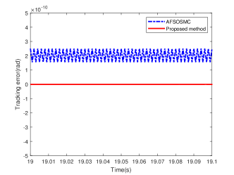
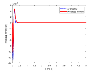
Fig. 2: (a)-(d) show the experimental results. Fig. 2: (a) and (c) demonstrate the responses of elevation angle tracking error by using INTSM-AFSOSMC and the proposed method, respectively. Fig. 2: (b) and (d) present the local magnification of corresponding tracking error to show the steady-state response more clearly. Fig. 2: (a) shows that elevation angle and pitch angel tracking errors converge to the origin in finite time by using our proposed control scheme as fast as the method in [24], which means our proposed method also possesses the characteristic of fast finite-time convergence. In addition, Fig. 2: (b) illustrates that the proposed method can weaken the chattering effect existing in the AFSOSMC method. A similar conclusion for the pitch angel tracking can be drawn in light of the Fig. 2: (c) and (d).

IV-B Experiment II: Attitude tracking control with time-varying lumped disturbances

For experiment II, the parameters of the both controller are as same as those in experiment I. The time-varying lumped disturbances are set as d1(t)=d2(t)=0.2sin(t)subscript𝑑1𝑡subscript𝑑2𝑡0.2𝑡{d_{1}}(t)={d_{2}}(t)=0.2\sin(t).

Refer to caption
(a) Response of elevation tracking error by AFSOSMC and proposed method
Refer to caption
(b) Local magnification of elevation tracking error
Refer to caption
(c) Response of pitch tracking error by AFSOSMC and proposed method
Refer to caption
(d) Local magnification of pitch tracking error
Figure 3: Results of experiment II

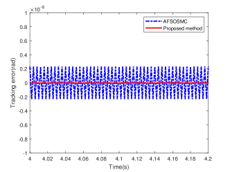
Fig. 3: (a)-(d) show the experimental results. Fig. 3: (a) and (c) illustrate the responses of elevation angle tracking error by using INTSM-AFSOSMC and the proposed method, respectively. Fig. 3: (b) and (d) present the local magnification of corresponding tracking error to show the steady-state response more clearly. From Fig. 3: (a) and (b), one can see that the proposed method can guarantee the fast finite-time uniformly ultimately boundedness coupled with large chattering suppression. However, the time-varying disturbance destroys the original property of finite-time convergence, which leads to the tracking errors only converging in a small neighborhood of the origin. A similar conclusion for the pitch angel tracking can be drawn in light of the Fig. 3: (c) and (d).

IV-C Experiment III: Performance analysis of the observer

For experiment III, we compare the performance of our proposed observer with the ASOSMO. The parameters of the proposed observer are set as m=3,k1=2,k2=2.5,k3=4,k4=30,κ=10formulae-sequence𝑚3formulae-sequencesubscript𝑘12formulae-sequencesubscript𝑘22.5formulae-sequencesubscript𝑘34formulae-sequencesubscript𝑘430𝜅10m=3,{k_{1}}=2,{k_{2}}=2.5,{k_{3}}=4,{k_{4}}=30,\kappa=10, and the ASOSMO adopts the same parameters except that m𝑚m is set as 222. To facilitate the comparison, we take the elevation angel tracking as an example and the time-varying disturbances is set as sin(t)𝑡\sin(t). Moreover, the following conventional sliding mode control method is selected as the control law

ut=g11(f1cte2ηsgn(st)ktst)subscript𝑢𝑡superscriptsubscript𝑔11subscript𝑓1subscript𝑐𝑡subscript𝑒2𝜂sgnsubscript𝑠𝑡subscript𝑘𝑡subscript𝑠𝑡{u_{t}}={g_{1}}^{-1}\left({-{f_{1}}-{c_{t}}{e_{2}}-\eta{\mathop{\rm sgn}}({s_{t}})-{k_{t}}{s_{t}}}\right) (67)

where the sliding mode surface st=e2+cte1subscript𝑠𝑡subscript𝑒2subscript𝑐𝑡subscript𝑒1{s_{t}}={e_{2}}+{c_{t}}{e_{1}} and ct=2,kt=0.5formulae-sequencesubscript𝑐𝑡2subscript𝑘𝑡0.5{c_{t}}=2,{k_{t}}=0.5, η𝜂\eta is set sufficiently large to ensure the stability of the helicopter system.
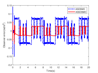
Refer to caption
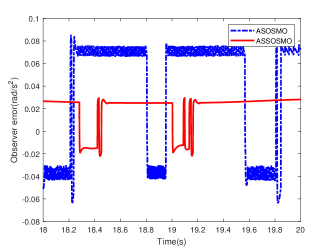
(a) Disturbance estimation error by using ASOSMO and ASSOSMO
Refer to caption
(b) Local magnification of disturbance estimation error
Figure 4: Results of experiment III

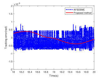
Fig. 4: (a)-(b) show the experimental results. Fig. 4: (a) illustrates the response of observer estimation error by using ASOSMO and the proposed observer and Fig. 4: (b) present the local magnification to show the response more clearly. From Fig. 4: (a) and (b), one can see that the estimation error can fast converge to a region of the origin in finite time by using our proposed observer. Furthermore, the proposed observer can effectively attenuate chattering existing in the ASOSMO and provide a more accurate and smoother output for the disturbance estimation.

V Conclusion

In this paper, a novel smooth adaptive fast second-order sliding mode control algorithm has been proposed. According to the types of disturbances, the design process of helicopter attitude tracking controllers can be divided into two parts. For the system with constant disturbances, a control scheme, consisting of a non-singular integral sliding mode surface and a novel smooth adaptive fast second-order sliding mode control, is proposed to achieve the fast finite-time convergence. For the system with the time-varying lumped disturbances, the control scheme can realize the fast finite-time uniformly ultimately boundedness. A novel adaptive-gain smooth second-order sliding mode observer is also present to estimate disturbances with a smooth output. The comparative simulation experiments are performed to demonstrate the effectiveness and superiority of the proposed control scheme with fast finite-time convergence, adaptation to disturbances, and chattering suppression for the attitude tracking of the 3-DOF helicopter system.

References

  • [1] Y. Zou and Z. Zheng, “A robust adaptive RBFNN augmenting backstepping control approach for a model-scaled helicopter,” IEEE Transactions on Control Systems Technology, vol. 23, no. 6, pp. 2344–2352, 2015.
  • [2] Z. Li, H. H. T. Liu, B. Zhu, H. Gao, and O. Kaynak, “Nonlinear robust attitude tracking control of a table-mount experimental helicopter using output feedback,” IEEE Transactions on Industrial Electronics, vol. 62, no. 9, pp. 5665–5676, 2015.
  • [3] B. Zheng and Y. Zhong, “Robust attitude regulation of a 3-DOF helicopter benchmark: Theory and Experiments,” IEEE Transactions on Industrial Electronics, vol. 58, no. 2, pp. 660–670, 2011.
  • [4] H. Liu, G. Lu, and Y. Zhong, “Robust LQR attitude control of a 3-DOF laboratory helicopter for aggressive maneuvers,” IEEE Transactions on Industrial Electronics, vol. 60, no. 10, pp. 4627–4636, 2013.
  • [5] R. I. Boby, H. Mansor, T. S. Gunawan, and S. Khan, “Robust adaptive LQR control of nonlinear system application to 3-DOF flight control system,” in 2014 IEEE International Conference on Smart Instrumentation, Measurement and Applications (ICSIMA), pp. 1–4, 2014.
  • [6] H. Castañeda, F. Plestan, A. Chriette, and J. de León-Morales, “Continuous differentiator based on adaptive second-order sliding-mode control for a 3-DOF helicopter,” IEEE Transactions on Industrial Electronics, vol. 63, no. 9, pp. 5786–5793, 2016.
  • [7] F. Kara and M. U. Salamci, “Controller design for a nonlinear 3-DOF helicopter model using adaptive sliding surfaces,” in 2019 XXVII International Conference on Information, Communication and Automation Technologies (ICAT), pp. 1–6, 2019.
  • [8] E. Vázquez, U. Pérez, and D. Hernández, “Continuous sliding-mode controllers for a 3-DOF helicopter,” in 2017 14th International Conference on Electrical Engineering, Computing Science and Automatic Control (CCE), pp. 1–6, 2017.
  • [9] X. Yang and X. Zheng, “Adaptive NN backstepping control design for a 3-DOF helicopter: Theory and Experiments,” IEEE Transactions on Industrial Electronics, vol. 67, no. 5, pp. 3967–3979, 2020.
  • [10] M. Chen, P. Shi, and C. Lim, “Adaptive neural fault-tolerant control of a 3-DOF model helicopter system,” IEEE Transactions on Systems, Man, and Cybernetics: Systems, vol. 46, no. 2, pp. 260–270, 2016.
  • [11] Y. Chen, X. Yang, and X. Zheng, “Adaptive neural control of a 3-DOF helicopter with unknown time delay,” Neurocomputing, vol. 307, no. SEP.13, pp. 98–105, 2018.
  • [12] S. Zeghlache, T. Benslimane, and A. Bouguerra, “Active fault tolerant control based on interval type-2 fuzzy sliding mode controller and nonlinear adaptive observer for 3-DOF laboratory helicopter,” ISA Transactions, pp. 280–303, 2017.
  • [13] Levant and Arie, “Higher-order sliding modes, differentiation and output-feedback control,” International Journal of Control, vol. 76, no. 9-10, pp. 924–941, 2003.
  • [14] J. A. Moreno and M. Osorio, “A Lyapunov approach to second-order sliding mode controllers and observers,” in 2008 47th IEEE Conference on Decision and Control, pp. 2856–2861, 2008.
  • [15] Y. Shtessel, M. Taleb, and F. Plestan, “A novel adaptive-gain supertwisting sliding mode controller: Methodology and application,” Automatica, vol. 48, no. 5, pp. 759 – 769, 2012.
  • [16] S. Laghrouche, J. Liu, F. S. Ahmed, M. Harmouche, and M. Wack, “Adaptive second-order sliding mode observer-based fault reconstruction for pem fuel cell air-feed system,” IEEE Transactions on Control Systems Technology, vol. 23, no. 3, pp. 1098–1109, 2015.
  • [17] Y. B. Shtessel, I. A. Shkolnikov, and A. Levant, “Smooth second-order sliding modes: Missile guidance application,” Automatica, vol. 43, no. 8, pp. 1470–1476, 2007.
  • [18] Q. Hu and B. Jiang, “Continuous finite-time attitude control for rigid spacecraft based on angular velocity observer,” IEEE Transactions on Aerospace and Electronic Systems, vol. 54, no. 3, pp. 1082–1092, 2018.
  • [19] Y. Hong, Y. Xu, and J. Huang, “Finite-time control for robot manipulators,” Systems & Control Letters, vol. 46, no. 4, pp. 243–253, 2002.
  • [20] A. F. Filippov, “Differential equations with discontinuous righthand sides,” Journal of Mathematical Analysis & Applications, vol. 154, no. 2, pp. 99–128, 1999.
  • [21] S. P. Bhat and D. S. Bernstein, “Continuous finite-time stabilization of the translational and rotational double integrators,” IEEE Transactions on Automatic Control, vol. 43, no. 5, pp. 678–682, 1998.
  • [22] Z. Zhu, Y. Xia, and M. Fu, “Attitude stabilization of rigid spacecraft with finite time convergence,” International Journal of Robust and Nonlinear Control, vol. 21, no. 6, pp. 686–702, 2011.
  • [23] S. Yu, X. Yu, B. Shirinzadeh, and Z. Man, “Continuous finite-time control for robotic manipulators with terminal sliding mode,” Automatica, vol. 41, no. 11, pp. 1957–1964, 2005.
  • [24] X.-T. Tran and H. Oh, “Prescribed performance adaptive finite-time control for uncertain horizontal platform systems,” ISA Transactions, vol. 103, pp. 122 – 130, 2020.